7 algebraic reconstruction algorithms

7 Algebraic Reconstruction Algorithms

An entirely different approach for tomographic imaging consists of assuming that the cross section consists of an array of unknowns, and then setting up algebraic equations for the unknowns in terms of the measured projection data. Although conceptually this approach is much simpler than the transform-based methods discussed in previous sections, for medical applications it lacks the accuracy and the speed of implementation. However, there are situations where it is not possible to measure a large number of projections, or the projections are not uniformly distributed over 180 or 360”) both these conditions being necessary requirements for the transform- based techniques to produce results with the accuracy desired in medical imaging. An example of such a situation is earth resources imaging using cross-borehole measurements discussed in Chapter 4. Problems of this type are sometimes more amenable to solution by algebraic techniques. Algebraic techniques are also useful when the energy propagation paths between the source and receiver positions are subject to ray bending on account of refraction, or when the energy propagation undergoes attenuation along ray paths as in emission CT. [Unfortunately, many imaging problems where refraction is encountered also suffer from diffraction effects (see Chap. 4).] As will be obvious from the discussion to follow, in algebraic methods it is essential to know ray paths that connect the corresponding transmitter and receiver positions. When refraction and diffraction effects are substantial (medium inhomogeneities exceed 10% of the average background value and the correlation length of these inhomogeneities is comparable to a wavelength), it becomes impossible to predict these ray paths. If algebraic techniques are applied under these conditions, we often obtain meaningless results.

If the refraction and diffraction effects are small (medium inhomogeneities are less than 2 to 3% of the average background value and the correlation width of these inhomogeneities is much greater than a wavelength), in some cases it is possible to combine algebraic techniques with digital ray tracing techniques [And82], [And84a], [And84b] and devise iterative procedures in which we first construct an image ignoring refraction, then trace rays connecting the corresponding transmitter and receiver locations through this distribution, and finally use these rays to construct a more accurate set of

ALGEBRAIC RECONSTRUCTION ALGORITHMS 275

algebraic equations. Experimental verification of this iterative procedure for weakly refracting objects has been obtained [And84b].

Space limitations prevent us from discussing here the combined ray tracing and algebraic reconstruction algorithms. Our aim in this section is to merely introduce the reader to the algebraic approach for image reconstruction. First we will show how we may construct a set of linear equations whose unknowns are elements of the object cross section. The Kaczmarz method for solving these equations will then be presented. This will be followed by the various approximations that are used in this method to speed up its computer implementation.

7.1 Image and Projection Representation

Fig. 7.1: In algebraic methods a square grid is superimposed over the unknown image. Image values are assumed to be constant within each cell of the grid. (From [Ros82].)

In Fig. 7.1 we have superimposed a square grid on the image f(x, y); we will assume that in each cell the function& y) is constant. Let fj denote this constant value in the jth cell, and let N be the total number of cells. For algebraic techniques a ray is defined somewhat differently. A ray is now a “fat” line running through the (x, y)-plane. To illustrate this we have shaded the ith ray in Fig. 7.1, where each ray is of width r. In most cases the ray width is approximately equal to the image cell width. A line integral will now be called a ray-sum.

Like the image, the projections will also be given a one-index representa-

wji for this cell = erea or ABC a2

276 COMPUTERIZED TOMOGRAPHIC IMAGING

tion. Let pi be the ray-sum measured with the ith ray as shown in Fig. 7.1. The relationship between the 4’s and pi’s may be expressed as

2 Wijfj=Pi, i=l, 2, “‘,M (1) j=l

where M is the total number of rays (in all the projections) and Wij is the weighting factor that represents the contribution of the jth cell to the ith ray integral. The factor Wij is equal to the fractional area of the jth image cell intercepted by the ith ray as shown for one of the cells in Fig. 7.1. Note that most of the wij’s are zero since only a small number of cells contribute to any given ray-sum.

If M and N were small, we could use conventional matrix theory methods to invert the system of equations in (1). However, in practice N may be as large as 65,000 (for 256 x 256 images), and, in most cases for images of this size, M will also have the same magnitude. For these values of M and N the size of the matrix [ Wij J in (1) is 65,000 X 65,000 which precludes any possibility of direct matrix inversion. Of course, when noise is present in the measurement data and when A4 < N, even for small Nit is not possible to use direct matrix inversion, and some least squares method may have to be used. When both M and N are large, such methods are also computationally impractical.

For large values of M and N there exist very attractive iterative methods for solving (1). These are based on the “method of projections” as first proposed by Kaczmarz [Kac37], and later elucidated further by Tanabe [Tan71]. To explain the computational steps involved in these methods, we first write (1) in an expanded form:

wllfl + w12f2+ w13f3+ ’ ” + wINfN=Pl

w21f1+ w22f2 + + * ’ ’ + w2NfN=tt)2

wMlfl+wM2f2+ +“‘+wMNfN=PM. (2)

A grid representation with N cells gives an image N degrees of freedom. Therefore, an image, represented by (f,, f2, + * * , fN), may be considered to be a single point in an N-dimensional space. In this space each of the above equations represents a hyperplane. When a unique solution to these equations exists, the intersection of all these hyperplanes is a single point giving that solution. This concept is further illustrated in Fig. 7.2 where, for the purpose of display, we have considered the case of only two variables f, and f2

satisfying the following equations:

wf1+ W12f2=P1

W2lfi + w22f2 ‘P2. (3)


initial guess

Fig. 7.2: The Kaczmarz method of solving algebraic equations is illustrated for the case of two unknowns. One starts with some arbitrary initial guess and then projects onto the line corresponding to the first equation. The resulting point is now projected onto the line representing the second equation. If there are only two equations, this process is continued back and forth, as illustrated by the dots in the figure, until convergence is achieved. (From [Ros82].)

The computational procedure for locating the solution in Fig. 7.2 consists of first starting with an initial guess, projecting this initial guess on the first line, reprojecting the resulting point on the second line, and then projecting back onto the first line, and so forth. If a unique solution exists, the iterations will always converge to that point.

For the computer implementation of this method, we first make an initial guess at the solution. This guess, denoted by f \O), f i”), * * * , f$, is represented vectorially by 7”) in the N-dimensional space. In most cases, we simply assign a value of zero to all the fi’S. This initial guess is projected on the hyperplane represented by the first equation in (2) givingpl), as illustrated in Fig. 7.2 for the two-dimensional case. p’) is projected on the hyperplane represented by the second equation in (2) to yieldp2) and so on. When?‘- *) is projected on the hyperplane represented by the ith equation to yield?‘), the process can be mathematically described by

(4)

where 4 = (Wii, Wi2, **a, WiN), and $i* i?i is the dot product of $i with itself. To see how (4) comes about we first write the first equation of (2) as


Fig. 7.3: The hyperplane w’, .p follows: = PI (represented by a Iine in this two-dimensional figure) is w’, * T=p,. (5) perpendicular to the vector w’,. (From fRos82J.) The hyperplane represented by this equation is perp+icular to the vector

w’, . This is illustrated in Fig. 7.3, where the vector OD_ represents i& . This equation simply says that the projection of a vector OC (for any point C on the hyperplane) on the vector w’t is of constant length. The unit vector or/’ along w’, is given by

(‘5)

and the perpendicular distance of the hyperplane from the origin, which is


-. equal to the length of OA m Fig. 7.3, is given by z &

(7)

Now to get To) we have to subtract from p”) the vector a

jw +o) -HZ (8)

where the length of the vector s is given by

pzI=Io~-lal

=3(O) * z- 1 Z(. (9) Substituting (6) and (7) in this equation, we get

(10)

Since the direction of zis the same as that of the unit vector z, we can write

z= IsI ou’= 3 (0) . - _ wlTpl w’,. WI * WI

(11)

Substituting (11) in (8), we get (4). As mentioned before, the computational procedure for algebraic recon-

struction consists of starting with an initial guess for the solution, taking successive projections on the hyperplanes represented by the equations in (2), eventually yielding PM). In the next iteration, PM) is projected on the hyperplane represented by the first equation in (2), and then successively onto the rest of the hyperplanes in (2), to yieldr2M), and so on. Tanabe [Tan711 has shown that if there exists a unique solutionx to the system of equations GY, then

lim 3ckM) =x . (12) k-m

A few comments about the convergence of the algorithm are in order here. If in Fig. 7.2 the two hyperplanes are perpendicular to each other, the reader may easily show that given for an initial guess any point in the (fi, fz)-plane, it is possible to arrive at the correct solution in only two steps like (4). On the other hand, if the two hyperplanes have only a very small angle between them, k in (12) may acquire a large value (depending upon the initial guess) before the correct solution is reached. Clearly the angles between the


hyperplanes considerably influence the rate of convergence to the solution. If the M hyperplanes in (2) could be made orthogonal with respect to one another, the correct solution would be arrived at with only one pass through the A4 equations (assuming a unique solution does exist). Although theoretically such orthogonalization is possible using, for example, the Gram-Schmidt procedure, in practice it is computationally not feasible. Full orthogonalization will also tend to enhance the effects of the ever present measurement noise in the final solution. Ramakrishnan et al. [Ram791 have suggested a pairwise orthogonalization scheme which is computationally easier to implement and at the same time considerably increases the speed of convergence. A simpler technique, first proposed in [Hou72] and studied in [Sla85], is to carefully choose the order in which the hyperplanes are considered. Since each hyperplane represents a distinct ray integral, it is quite likely that adjacent ray integrals (and thus hyperplanes) will be nearly parallel. By choosing hyperplanes representing widely separated ray integrals, it is possible to improve the rate of convergence of the Kaczmarz approach.

A not uncommon situation in image reconstruction is that of an overdetermined system in the presence of measurement noise. That is, we may have M > N in (2) and pl, p2, . . . , pm corrupted by noise. No unique solution exists in this case. In Fig. 7.4 we have shown a two-variable system represented by three “noisy” hyperplanes. The broken line represents the course of the solution as we successively implement (4). Now the “solution” doesn’t converge to a unique point, but will oscillate in the neighborhood of the intersections of the hyperplanes.

When M < N a unique solution of the set of linear equations in (2) doesn’t exist, and, in fact, an infinite number of solutions are possible. For example, suppose we have only the first of the two equations in (3) to use for calculating the two unknowns f, and f2; then the solution can be anywhere on the line corresponding to this equation. Given the initial guess PO) (see Fig. 7.3), the best one could probably do under the circumstances would be to draw a projection from p”) on this line, and call the resulting 3c1) a solution. Note that the solution obtained in this manner corresponds to that point on the line which is closest to the initial guess. This result has been rigorously proved by Tanabe [Tan711 who has shown that when M < N, the iterative approach described above converges to a solution, call it 3;) such that IPO’ - 3;l is minimized.

Besides its computational efficiency, another attractive feature of the iterative approach presented here is that it is now possible to incorporate into the solution some types of a priori information about the image one is reconstructing. For example, if it is known a priori that the image f (x, y) is nonnegative, then in each of the solutionsJt(k), successively obtained by using (4), one may set the negative components equal to zero. One may similarly incorporate the information that f (x, v) is zero outside a certain area, if this is known.


Fig. 7.4: Illustrated here is the case when the number of equations is greater than the number of unknowns. The lines don’t intersect at a single unique point, because the observations p,. p2, p, have been assumed to be corrupted by noise. No unique solution exists in this case, and the final solution will oscillate in the neighborhood of intersections of the three lines. (From [Ros82].)

In applications requiring a large number of views and where large-sized reconstructions are made, the difficulty with using (4) can be in the calculation, storage, and fast retrieval of the weight coefficients w,. Consider the case where we wish to reconstruct an image on a 100 x 100 grid from 100 projections with 150 rays in each projection. The total number of weights, w,, needed in this case is 108, which is an enormous number and can pose problems in fast storage and retrieval in applications where reconstruction speed is important. This problem is somewhat eased by making approximations, such as considering WV, to be only a function of the perpendicular distance between the center of the ith ray and the center of the jth cell. This perpendicular distance can then be computed at run time.

To get around the implementation difficulties caused by the weight coefficients, a myriad of other algebraic approaches have also been suggested, many of which are approximations to (4). To discuss some of the more implementable approximations, we first recast (4) in a slightly different


form:

f(i) =f(i- 1) + pi wij J J

i wt k=L

where

qi=T(i- 1) . q

(13)

k=l

(15)

These equations say that when we project the (i - 1)th solution onto the ith hyperplane [ ith equation in (2)] the gray level of the jth element, whose current value is f!‘- l)

J ’ is obtained by correcting its current value by AJJ’),

where

Note that while pi is the measured ray-sum along the ith ray, qi may be considered to be the computed ray-sum for the same ray based on the (i - 1)th solution for the image gray levels. The correction Af, to the jth cell is obtained by first calculating the difference between the measured ray-sum and the computed ray-sum, normalizing this difference by CF==, w&, and then assigning this value to all the image cells in the ith ray, each assignment being weighted by the corresponding w,.

With the preliminaries presented above, we will now discuss three different computer implementations of algebraic algorithms. These are represented by the acronyms ART, SIRT, and SART.

7.2 ART (Algebraic Reconstruction Techniques)

In many ART implementations the wik’s in (16) are simply replaced by l’s and O’s, depending upon whether the center of the kth image cell is within the ith ray. This makes the implementation easier because such a decision can easily be made at computer run time. In this case the denominator in (16) is given by CF==, wi = Ni which is the number of image cells whose centers are within the ith ray. The correction to the jth image cell from the ith equation in (2) may now be written as

Af(‘) mpi- qi J

Ni (17)


for all the cells whose centers are within the ith ray. We are essentially smearing back the difference (pi - qi)/Ni over these image cells. In (17), qi’s are calculated using the expression in (15), except that one now uses the binary approximation for wik’s.

The approximation in (17), although easy to implement, often leads to artifacts in the reconstructed images, especially if Ni isn’t a good approximation to the denominator. Superior reconstructions may be obtained if (17) is replaced by

Afji)=pi-?% Li Ni

where Li is the length (normalized by 6, see Fig. 7.1) of the ith ray through the reconstruction region.

ART reconstructions usually suffer from salt and pepper noise, which is caused by the inconsistencies introduced in the set of equations by the approximations commonly used for Wik’s. The result is that the computed ray- sums in (15) are usually poor approximations to the corresponding measured ray-sums. The effect of such inconsistencies is exacerbated by the fact that as each equation corresponding to a ray in a projection is taken up, it changes some of the pixels just altered by the preceding equation in the same projection. The SIRT algorithm described briefly below also suffers from these inconsistencies in the forward process [appearing in the computation of qi’s in (16)], but by eliminating the continual and competing pixel update as each new equation is taken up, it results in smoother reconstructions.

It is possible to reduce the effects of this noise in ART reconstructions by relaxation, in which we update a pixel by o * AJ;‘), where (Y is less than 1. In some cases, the relaxation parameter (Y is made a function of the iteration number; that is, it becomes progressively smaller with increase in the number of iterations. The resulting improvements in the quality of reconstruction are usually at the expense of convergence.

7.3 SIRT (Simultaneous Iterative Reconstructive Technique)

In this approach, which at the expense of slower convergence usually leads to better looking images than those produced by ART, we again use (17) or (18) to compute the change Afji) in the jth pixel caused by the ith equation in (2). However, the value of the jth cell isn’t changed at this time. Before making any changes, we go through all the equations, and then only at the end of each iteration are the cell values changed, the change for each cell being the average value of all the computed changes for that cell. This constitutes one iteration of the algorithm. In the second iteration, we go back to the first equation in (2) and the process is repeated.


7.4 SART (Simultaneous Algebraic Reconstruction Technique)

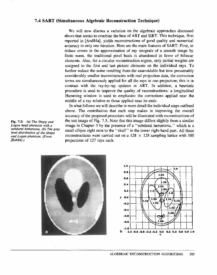
We will now discuss a variation on the algebraic approaches discussed above that seems to combine the best of ART and SIRT. This technique, first reported in [And84a], yields reconstructions of good quality and numerical accuracy in only one iteration. Here are the main features of SART: First, to reduce errors in the approximation of ray integrals of a smooth image by finite sums, the traditional pixel basis is abandoned in favor of bilinear elements. Also, for a circular reconstruction region, only partial weights are assigned to the first and last picture elements on the individual rays. To further reduce the noise resulting from the unavoidable but now presumably considerably smaller inconsistencies with real projection data, the correction terms are simultaneously applied for all the rays in one projection; this is in contrast with the ray-by-ray updates in ART. In addition, a heuristic procedure is used to improve the quality of reconstructions: a longitudinal Hamming window is used to emphasize the corrections applied near the middle of a ray relative to those applied near its ends.

In what follows we will describe in more detail the individual steps outlined above. The contribution that each step makes in improving the overall accuracy of me proposed procedure will be illustrated with reconstructions of

Fig. 7.5: (a) The Shepp and the test image of Fig. 7.5. Note that this image differs slightly from a similar Logan head phantom with a subdural hematoma. (b) The gray

image in Chapter 3 by the presence of a “

subdural

hematoma,

”

which is a

level distribution of the Shepp small ellipse right next to the “

skull

”

in the lower right-hand part. All these and Logan phantom. (From reconstructions were carried out on a 128 x 128 sampling lattice with 100 [Kak84J.) projections of 127 rays each.

b -1.0-0.8 -0.a -0.4 -0.2 0.0 0.2 0.4 0.0 0.8 1.0 x


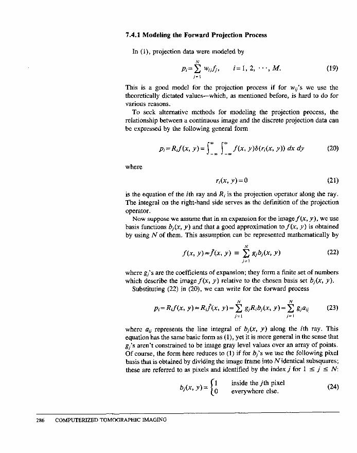
7.4.1 Modeling the Forward Projection Process

In (l), projection data were modeled by

Pi=5 wijfi9 i=l, 2, -**, M. j=l

(19)

This is a good model for the projection process if for Wij’s we use the theoretically dictated values-which, as mentioned before, is hard to do for various reasons.

To seek alternative methods for modeling the projection process, the relationship between a continuous image and the discrete projection data can be expressed by the following general form

Pi=Rif(X, I’)= Sy, lr, f(X, y)G(ri(X, y)) dx dy (20)

where

ri(X, Y)=O (21)

is the equation of the ith ray and Ri is the projection operator along the ray. The integral on the right-hand side serves as the definition of the projection operator.

Now suppose we assume that in an expansion for the imagef(x, y), we use basis functions bj(x, y) and that a good approximation tof(x, y) is obtained by using N of them. This assumption can be represented mathematically by

f(X, Y)=ftXs Y) E 5 gjbjCx, Y) (22) j=l

where gj’s are the coefficients of expansion; they form a finite set of numbers which describe the image f(x, y) relative to the chosen basis set bj(X, y).

Substituting (22) in (20), we can write for the forward process

Pi=Rif(x, Y)F”RJ(X, Y)=g gjRibj(x, Y)=i &au j=l j=l

(23)

where a, represents the line integral of bj(X, y) along the ith ray. This equation has the same basic form as (l), yet it is more general in the sense that gi’s aren’t constrained to be image gray level values over an array of points. Of course, the form here reduces to (1) if for bj’s we use the following pixel basis that is obtained by dividing the image frame into N identical subsquares; these are referred to as pixels and identified by the index j for 1 5 j 5 N:

bj(x, Y)= I

1 inside the jth pixel o everywhere else. (24)


In keeping with the nature of J’s in (l), gj’s with these basis functions represent the average off (x, y) over the jth pixel and Ribj(X, y) represents the length of the intersection of tbe ith ray with the jth pixel. Although (20) implies rays of zero width, if we now associate a finite width with each ray, the elements of the projection matrix will represent the areas of intersection of these ray strips with the pixels.

In SART, superior reconstructions are obtained by using a model of the forward projection process that is more accurate than what can be obtained by the choice of pixel basis functions-this is done by using bilinear elements which are the simplest higher order basis functions. The basis functions obtained from bilinear elements are pyramid shaped, each with a support extending over a square region the size of four pixels. It can be shown that the gj’s appearing in (22) for the case of bilinear elements are the sample values of the image functionf(x, y) on a square lattice. It can further be shown that whereas the pixel basis leads to a discontinuous image representation, the bilinear elements allow a continuous form of p(x, y) to be regenerated for computation. However, finding the exact ray integrals across such bilinear elements [as called for by Ribj(x, y) in (23)] for a large number of rays is a time-consuming task and we will use an approximation.

Rather than try to find separately the individual coefficients aij for a particular ray, we approximate the overall ray integral RJ(X, y) by a finite sum involving a set of Mi equidistant points {f^(sim)}, for 1 5 m I Mi

Fig. 7.6: The ray-sum equations for a set of equidistant points

[Lytl(O] (see Fig. 7.6):

along a straight line cut by the Mi circular reconstruction region. Pi” x J(Sim)AS* (25) (From [Kak84J.) m=l


The value f(Sim) is determined from the values gj of f(x, y) on the four neighboring points of the sampling lattice, i.e., by bilinear interpolation. We write

%(Sim) = i dijrngj for m= 1, 2, .a*, Mi. (26) j=1

The coefficient dti,,, is therefore the contribution that is made by the jth image sample to the mth point on the ith ray. Combining (25) and (26), we obtain an approximation to the ray integral pi as a linear function of the image samples gj:

m=l j=I

Mi

= 2 C dij,gjAS for 1lisJ j=l m=l

=i aijgj j=l

(27)

(28)

where the coefficients au represent the net effect of the linear transforma- tions. They are determined as the sum of the contributions from different points along the ray:

Mi aij= C dijmAS. (30)

m=l Therefore, au is proportional to the sum of contributions made by the jth image sample to all the points on the ith ray. It is important to the overall accuracy of the model that for m = 1 and for m = Mi, i.e., for the first and last points of the ray within the reconstruction circle, the weights are adjusted so that X7= i ab equals the actual physical length Li.

One certainly has latitude about selecting the step size As; setting it equal to half the spacing of the sampling lattice provides a good trade-off between the accuracy of representation and computational cost.

7.4.2 Implementation of the Reconstruction Algorithm

As mentioned before, the results of SART implementation will be shown on 128 x 128 matrices using 100 projections, each with 127 rays. In the model of (29), this corresponds to N = 16,384 picture elements and an overall number of rays I = 12,700. Note that the system of equations is underdetermined by about 25 % , but then the reconstruction circle covers only about 75% of the area of the square sampling lattice.

With the au’s determined by the method just described, the reader will now be taken through a series of steps that are part of the SART implementation.


First, it will be shown that even with the superior forward projection modeling by the use of bilinear elements, one doesn

’

t

want to carry out a sequential implementation of the reconstruction algorithm.

A sequential implementation can be carried out by using the update formula of (4), reexpressed here in terms of SART symbols:

(31)

Fig. 7.1: Reconstruction from one iteration of sequential ART. (a) Image. (b) Line plot through the three small tumors (for y = - 0.605). (From [And84a].)

where ZJ denotes the ith row vector of the array aij. As described before, the estimate g(k) of the image vector is updated after each ray has been considered. We set the initial estimate g

’

(O)

to zero, and we say that one iteration of the algebraic reconstruction technique is completed when all I rays, i.e., all I ray-sum equations, have been used exactly once. Owing to reasons discussed in Section 7.1, for sequential processing the projection data are ordered in such a manner that the angle between the projections considered successively is kept large; for the reconstructions shown here that were obtained with sequential updating, this angle was 73.8

”

.

Fig. 7.7(a) illustrates the reconstruction of the test image for one iteration of the sequential implementation. In order to avoid streak artifacts in the final image, the correction terms for the first few projections are de-emphasized relative to those for projections considered later on. The image has been thresholded to the gray level range 0.95-1.05 to illustrate the finer detail. Note that even the larger structures are buried in the salt and pepper noise present when no form of relaxation or smoothing is used. Fig. 7.7(b) shows a line plot through the three small tumors of the phantom (the profile shown is along the line y = - 0.605). We observe that the amplitude variations of the noise largely exceed the density differences characterizing these structures.

1.050.

1.037 -

1.025-

1.012.

1 .ooo* $

.9875'

.9750-

.9625 *

b .9500* I

- 1.00 -.750 - ,500 -.250 0.00 ,250 ,500 ,750


It will now be shown that superior results are obtained if instead of sequentially updating pixels on a ray-by-ray basis we simultaneously apply to a pixel the average of the corrections generated by all the rays in a projection. Stated in a bit more detail, this is what we want to do: For the first ray in a projection we compute as before the corrections to be made at every pixel. Instead of actually applying these corrections, we store them in a separate array to be called the correction array (the size of which is the same as that of the image array). Then we take up the next ray and add the pixel updates generated by this ray to the correction array. And then the next ray, and so on. After we are through all the rays in a projection, we add the correction array (or some fraction thereof) to the image array. This entire process is repeated with every projection. Fig. 7.8(a) illustrates the reconstruction obtained with this method. The precise formula that was used in the reconstruction in Fig. 7.8 for updating the pixel values can be stated as follows:

& I

g@+Lg~)+- J

1 p

i

- ,

‘

iTg

’

w

aij

i aij L ‘

=I

C aij (32)

Fig. 1.8: Reconstruction from one iteration of SART. (a) Image. (b) Line plot through the three small tumors (for y = - 0.605). (From [And84a].)

where the summation with respect to i is over the rays intersecting the jth image element for a given scan direction.

Compared to the reconstruction of Fig. 7.7 for the sequential scheme, the simultaneous method offers a reduction in the amplitude of the noise. In addition, the noise in the reconstructed image has become more slowly

1.050 1.050

1.037 1.037

1.025 1.025

1.012 1.012

1.000 1.000

.9875 - .9875 -

.9750 - .9750 -

.9625. .9625.

b .9500 1 .9500 7 I I

b -1.00 -.750 -.500 -.250 0.00 -1.00 -.750 -.500 -.250 0.00 .250 .250 .500 ,750 1 .500 ,750 1 00


Fig. 7.9: The longitudinal Hamming window for a set of straight rays. (From [And84a].)

undulating compared to the previous salt and pepper appearance. This technique maintains the rapid convergence of ART-type algorithms while at the same time it has the noise suppressing features of SIRT. AS with SIRT, the simultaneous implementation does require the storage of an additional array for the correction terms.

The last step, heuristic in nature, in SART consists of modifying the back- distribution of correction terms by a longitudinal Hamming window. The idea of the window is illustrated in Fig. 7.9. The uniform back-distribution according to the coefficients au is replaced by a weighted version. This corresponds to replacing the correction term

pi _ a’,T-g’(k) aij

fj aij

(33)

j=l

in (32) by a weighted correction term

*, pi - ZTzck)

” 5 Qij

(34)

j=l

where the weighting coefficients tij are given by [compare with (30)]

Mi tij= C hi,dij,AS*

m=l (35)

The sequence hi,, for 1 I m I A4i, is a Hamming window of length A4i. Note that the length of the window varies according to the number of points Mi describing the part of the ray inside the reconstruction circle.

The weighted back-distribution of corrections emphasizes the central portions of rays in relation to portions closer to the periphery. Fig. 7.10 illustrates a reconstruction of the test image after one iteration with the longitudinal window in conjunction with the simultaneous scheme previously described. We see an improvement over the reconstructions of Figs. 7.7 and 7.8: the noise is practically gone and all the structures can be fairly well distinguished. If we hadn’t applied the corrections in a simultaneous scheme but incorporated the longitudinal Hamming window only for the sequential implementation, we would have arrived at the noisy reconstruction illustrated in Fig. 7.11.

An important question that remains to be answered is: What happens when we go through iterations with, say, the simultaneous implementation; meaning that after we have made a reconstruction by going through all the projections once, we go through them all once again using the reconstruction of Fig. 7.10 as our initial solution; and then continue iterating in like fashion?


1.025.

1.012.

1.000.

.9875'

.9750.

.9625.

b .95000 -1.00 -.750 -.500 -.250 0.00 ,250 .500 ,750 .

Fig. 7.10: Reconstruct ion from one iteration of SART with a longitudinal Hamming window. (a) Image. (b) Line plot through the three small tumors (fbr y = - 0.605). (From [And84a].)

In Figs. 7.12 and 7.13, we have shown the reconstructions obtained with two and three iterations, respectively. As is evident from the reconstructions, we do gain more contrast, although at the cost of increased salt and pepper noise. All reconstructions shown represent the raw output from the algorithms with no postprocessing applied to suppress noise.

For the purpose of comparison, we have included in Fig. 7.14 the reconstruction obtained by using a convolution-backprojection algorithm. Comparing this with Fig. 7.10, we see that the SART reconstruction with one iteration is quite similar, although with further iterations, as displayed in Figs. 7.12 and 7.13, we see an increased amplitude of the salt and pepper noise, which is probably an indication of remaining inconsistencies in the model used for the forward projection process.

7.5 Bibliographic Notes

The earliest expositions on algebraic reconstruction were by Gordon et al. [Gor70], [Gor71], [Gor74], Herman et al. [Her71], [Her73], [Her77], and Budinger and Gullberg [Bud74]. The reader is also referred to the book by Herman [Her801 for an exhaustive treatment of the subject.

When binary values are chosen for the weights wU in (16) in ART, i.e., wg is set equal to 1 if the center of thejth pixel falls within the strip of the ith ray and 0 if not, it becomes necessary to adjust the width of each ray according to the orientation of the projection [Gor74], [Her73], [Opp75].

Attempts have been made to reduce the salt and pepper noise associated with ART-type reconstructions by increasing the number of rays per view [Smi77]. When the number of rays per view is increased, many pixels are


Fig. 7.11: Reconstruction from one iteration of sequential ART with a longitudinal Hamming window. (a) Image. (b) Line plot through the three small tumors (for y = -0.605). (From [AndBla].)

Fig. 7.12: Reconstruction from two iterations of SART with a longitudinal Hamming window. (a) Image. (b) Line plot through the three small tumors (for y = - 0.605). (From [And84a].)

1.050.

1.037.

1.025.

1.012.

1.000.

.9875-

.9750 -

.9625.

* b .""",.oo -.750 - I -.250 0.00 ,250 ,500 ,750 1.00

intersected by several rays in each projection. This results in the averaging of possible errors committed in the correction procedure such as the one given by (4). Common practice is to have a system with about four times as many equations as unknown pixel values [Her80], [Her78], [She74]. The computational cost, however, is increased directly with the number of rays processed. An additional method has been to use a relaxation factor h < 1 [Gor74], [Her80], [Her76], [Her78], [Hou72], [Swe73] which, although reducing the salt and pepper noise, increases the number of iterations required for convergence.

The SART algorithm was first reported in [And84a]. In contrast with the bilinear elements used for SART, the pixel basis is common to much

1.050

1.037 I

1.025.

1.012.

l .OOO-

.9875

.9750

.9625

,, .%oo !- -1.00 -.750 -

I . 00 -.250 0.00 ,250 .500 .750

I 00


Fig. 7.13: Reconstruction from three iterations of SART with a longitudinal Hamming window. (a) Image. (b) Line plot through the three small tumors (for y = - 0.605). (From /And84a].)

Fig. 7.14: Convolution-backprojection reconstruction of the test image. (a) Image. (b) Line plot through the three small tumors (for y = - 0.605). (From [And84a].)

1.050 1.050

I!

1.037 1.037

1.025 1.025

1.012 1.012

1.000 1.000

.9675 .9675

.9750

b::

.9625

b’ 9500 -1.00 -.750 -.500 -.250 0.00 ,250 ,500 .750 ,250 ,500 .750 IO

literature published on algebraic techniques [Din79], [Gi172], [Gor74], [Gor70], [HergO], [Her76], [Her78], [Her73], [Hou72], [Opp75], [She74].

The error-correcting procedure of the basic ART algorithm as given by (4) is discussed in [Gor74], [GonO], [HergO], [Her76], [Her78], [Her73], [Hou72].

As first shown by Hounsfield [Hou72], in order to improve the convergence of a sequential algebraic algorithm one should order the projections in such a manner that successive projections are well separated. This he justified on the basis of high correlation between the information in neighboring projections. Later the scheme was demonstrated to have a deeper

1.025 1

.9750.

9625.

b .9500~------ -1.00 -.750 -.500 -.250 0.00 ,250 .5(1 ,750 1 0


mathematical foundation as a tool for speeding up the convergence of ART- type algorithms. (The proof relies on a continuous formulation of ART, as shown by Hamaker and Solmon [Ham78].) Ramakrishnan et al. [Ram791 have shown how by orthogonalization of the algebraic equations we can increase the speed of convergence of a reconstruction algorithm.

The SIRT algorithm was first proposed by Gilbert [Gi172]. A simplified form of the simultaneous technique was used by Oppenheim in [Opp75]. However, the scope of the implementation as described by (32) is much wider. The method can be used advantageously in the general image reconstruction problem for curved rays with overlapping and nonoverlapping ray strips as well as in conjunction with any image representation, provided the forward process can be expressed in the form of (23).

A combination of algebraic reconstruction and digital ray tracing appears ideal for imaging lightly refracting objects [Cha79], [Chagl]. A survey of digital ray tracing and ray linking for this purpose is presented in [And82]. If a refracting object has special symmetries, then as shown by Vest [Ves75] it may be possible to reconstruct the object without ray tracing. The reader is referred to [And84b] for experimental demonstrations of how algebraic reconstruction can be combined with digital ray tracing for the cross-sectional imaging of lightly refracting objects.

7.6 References

[And821

[And84a]

[And84b]

[Bud741

[Cha79]

[ChaBl]

[Din791

[Gil721

@or701

[Gor’ll]

[Gor74]

[Ham781

[Her71 ]

A. H. Andersen and A. C. Kak, “Digital ray tracing in two-dimensional refractive fields,” J. Acoust. Sot. Amer., vol. 72, pp. 1593-1606, Nov. 1982. - “Simultaneous algebraic reconstruction technique (SART): A superior implementation of the art algorithm,” Ultrason. Imaging, vol. 6, pp. 81-94, Jan. 1984. -, “The application of ray tracing towards a correction for refracting effects in computed tomography with diffracting sources, ” TR-EE 84-14, School of Electrical Engineering, Purdue Univ., Lafayette, IN, 1984. T. F. Budinger and G. T. Gullberg, “Three-dimensional reconstruction in nuclear medicine emission imaging,” IEEE Trans. Nucl. Sci., vol. NS-21, pp. 2-21, 1974. S. Cha and C. M. Vest, “Interferometry and reconstruction of strongly refracting asymmetric-refractive-index fields,” Opt. Lett., vol. 4, pp. 311-313, 1979. -, “Tomographic reconstruction of strongly refracting fields and its application to interferometric measurements of boundary layers,” Appl. Opt., vol. 20, pp. 2787-2794, 1981. K. A. Dines and R. J. Lytle, “Computerized geophysical tomography,” Proc. IEEE, vol. 67, pp. 1065-1073, 1979. P. Gilbert, “Iterative methods for the reconstruction of three dimensional objects from their projections,” J. Theor. Biol., vol. 36, pp. 105-117, 1972. R. Gordon, R. Bender, and G. T. Herman, “Algebraic reconstruction techniques (ART) for three dimensional electron microscopy and X-ray photography,” J. Theor. Biol., vol. 29, pp. 471-481, 1970. R. Gordon and G. T. Herman, “Reconstruction of pictures from their projections,” Commun. Assoc. Comput. Mach., vol. 14, pp. 759-768, 1971. R. Gordon, “A tutorial on ART (algebraic reconstruction techniques),” IEEE Trans. Nucl. Sci., vol. NS-21, pp. 78-93, 1974. C. Hamaker and D. C. Solmon, “The angles between the null spaces of X rays,” J. Math. Anal. Appl., vol. 62, pp. l-23, 1978. G. T. Herman and S. Rowland, “Resolution in ART: An experimental investigation


[Her731

[Her761

[Her771

[Her781

[Her801

[Hot1721

[Kac37]

WW

[WOI

topp751

[Ram791

[Ros82]

[She741

[Sla85]

[Smi77]

[Swe73]

[Tan7 l]

[Ves75]

ofthe resolving power of an algebraic picture reconstruction,” J. Theor. Biol., vol. 33, pp. 213-233, 1971. G. T. Herman, A. Lent, and S. Rowland, “ART: Mathematics and applications: A report on tlte mathematical foundations and on applicability to real data of the algebraic reconstruction techniques,” J. Theor. Biol., vol. 43, pp. l-32, 1973. G. T. Herman and A. Lent, “Iterative reconstruction algorithms,” Comput. Biol. Med., vol. 6, pp. 273-294, 1976. G. T. Herman and A. Naparstek, “Fast image reconstruction based on a Radon inversion formula appropriate for rapidly collected data,” SIAM J. Appl. Math., vol. 33, pp. 511-533, Nov. 1977. G. T. Herman, A. Lent, and P. H. Lutz, “Relaxation methods for image reconstruction,” Commun. A.C.M., vol. 21, pp. 1.52-158, 1978. G. T. Herman, Image Reconstructions from Projections. New York, NY: Academic Press, 1980. G. N. Hounstield, “A method of and apparatus for examination of a body by radiation such as x-ray or gamma radiation,” Patent Specification 1283915, The Patent Office, 1972. S. Kaczmarz, “Angenaherte auflosung von systemen linearer gleichungen,” Bull. Acad. Pol. Sci. Lett. A, vol. 6-8A, pp. 355-357, 1937. A. C. Kak, “Image reconstructions from projections, ” in Digitallmage Processing Techniques, M. P. Ekstrom, Ed. New York, NY: Academic Press, 1984. R. J. Lytle and K. A. Dines, “Iterative ray tracing between boreholes for underground image reconstruction,” IEEE Trans. Geosciences and Remote Sensing, vol. GE-18, pp. 234-240, 1980. B. E. Oppenheim, “Reconstruction tomography from incomplete projections,” in Reconstruction Tomography in Diagnostic Radiology and Nuclear Medicine, M. M. Ter Pogossian et al., Eds. Baltimore, MD: University Park Press, 1975. R. S. Ramakrishnan, S. K. Mullick, R. K. S. Rathore, and R. Subramanian, “Orthogonalization, Bernstein polynomials, and image restoration,” Appl. Opt., vol. 18, pp. 464-468, 1979. A. Rosenfeld and A. C. Kak, Digital Picture Processing, 2nd ed. New York, NY: Academic Press, 1982. L. S. Shepp and B. F. Logan, “The Fourier reconstruction of a head section,” IEEE Trans. Nucl. Sci., vol. NS-21, pp. 21-43, 1974. M. Slaney and A. C. Kak, “Imaging with diffraction tomography,” TR-EE 85-5, School of Electrical Engineering, Purdue Univ., Lafayette, IN, 1985. K. T. Smith, D. C. Salmon, and S. L. Wagner, “Practical and mathematical aspects of the problem of reconstructing objects from radiographs,” Bull. Amer. Math. Sot., vol. 83, pp. 1227-1270, 1977. D. W. Sweeney and C. M. Vest, “Reconstruction of three-dimensional refractive index fields from multi-directional interferometric data,” Appl. Opt., vol. 12, pp. 1649-1664, 1973. K. Tanabe, “Projection method for solving a singular system,” Numer. Math., vol. 17, pp. 203-214, 1971. C. M. Vest, “Interferometry of strongly refracting axisymmetric phase objects,” Appl. Opt., vol. 14, pp. 1601-1606, 1975.


7 algebraic reconstruction algorithms

Documents