7 associative memory networks related to/based on...

Intro. Comp. NeuroSci. — Ch. 7 September 7, 2005

7 Associative Memory NetworksRelated to/based on Lytton’s Chapter 10.

7.1 Introductory concepts

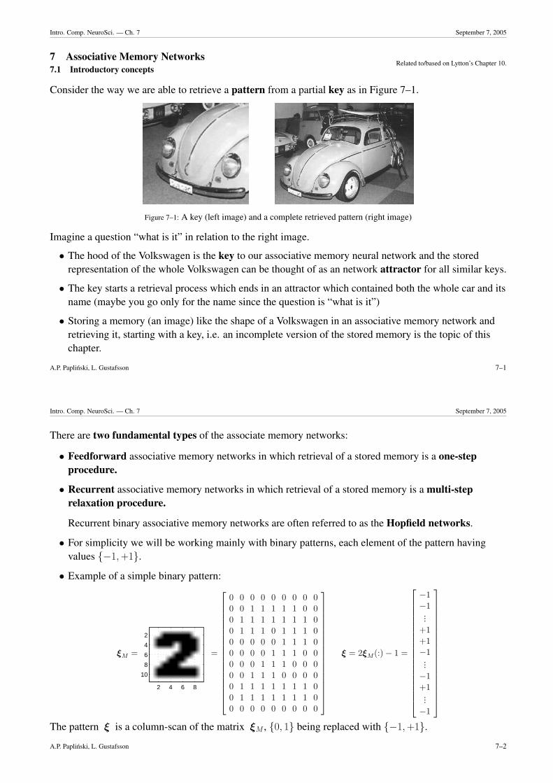
Consider the way we are able to retrieve a pattern from a partial key as in Figure 7–1.

Figure 7–1: A key (left image) and a complete retrieved pattern (right image)

Imagine a question “what is it” in relation to the right image.

• The hood of the Volkswagen is the key to our associative memory neural network and the storedrepresentation of the whole Volkswagen can be thought of as an network attractor for all similar keys.

• The key starts a retrieval process which ends in an attractor which contained both the whole car and itsname (maybe you go only for the name since the question is “what is it”)

• Storing a memory (an image) like the shape of a Volkswagen in an associative memory network andretrieving it, starting with a key, i.e. an incomplete version of the stored memory is the topic of thischapter.

A.P. Paplinski, L. Gustafsson 7–1


There are two fundamental types of the associate memory networks:

• Feedforward associative memory networks in which retrieval of a stored memory is a one-stepprocedure.

• Recurrent associative memory networks in which retrieval of a stored memory is a multi-steprelaxation procedure.

Recurrent binary associative memory networks are often referred to as the Hopfield networks.

• For simplicity we will be working mainly with binary patterns, each element of the pattern havingvalues {−1, +1}.

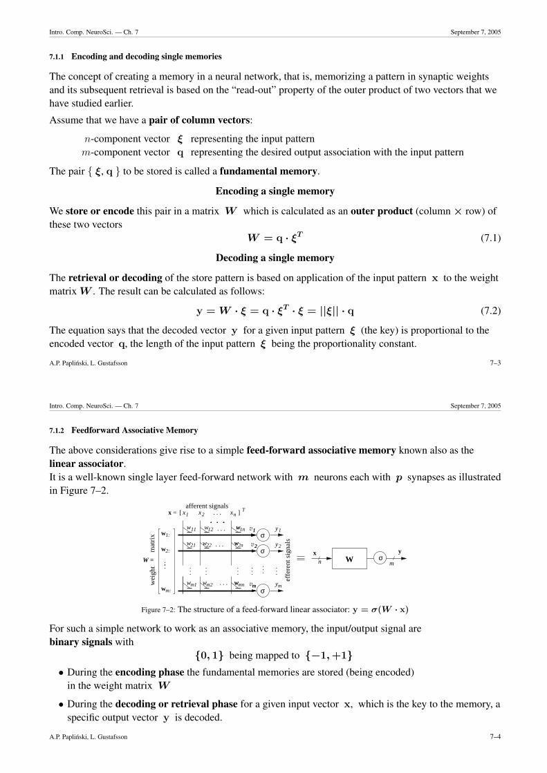
• Example of a simple binary pattern:

ξM =

2 4 6 8

2

4

6

8

10

=

0 0 0 0 0 0 0 0 00 0 1 1 1 1 1 0 00 1 1 1 1 1 1 1 00 1 1 1 0 1 1 1 00 0 0 0 0 1 1 1 00 0 0 0 1 1 1 0 00 0 0 1 1 1 0 0 00 0 1 1 1 0 0 0 00 1 1 1 1 1 1 1 00 1 1 1 1 1 1 1 00 0 0 0 0 0 0 0 0

ξ = 2ξM(:)− 1 =

−1−1

...+1+1−1

...−1+1

...−1

The pattern ξ is a column-scan of the matrix ξM , {0, 1} being replaced with {−1, +1}.



7.1.1 Encoding and decoding single memories

The concept of creating a memory in a neural network, that is, memorizing a pattern in synaptic weightsand its subsequent retrieval is based on the “read-out” property of the outer product of two vectors that wehave studied earlier.

Assume that we have a pair of column vectors:

n-component vector ξ representing the input patternm-component vector q representing the desired output association with the input pattern

The pair { ξ, q } to be stored is called a fundamental memory.

Encoding a single memory

We store or encode this pair in a matrix W which is calculated as an outer product (column × row) ofthese two vectors

W = q · ξT (7.1)

Decoding a single memory

The retrieval or decoding of the store pattern is based on application of the input pattern x to the weightmatrix W . The result can be calculated as follows:

y = W · ξ = q · ξT · ξ = ||ξ|| · q (7.2)

The equation says that the decoded vector y for a given input pattern ξ (the key) is proportional to theencoded vector q, the length of the input pattern ξ being the proportionality constant.



7.1.2 Feedforward Associative Memory

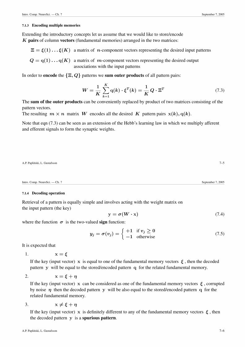
The above considerations give rise to a simple feed-forward associative memory known also as thelinear associator.It is a well-known single layer feed-forward network with m neurons each with p synapses as illustratedin Figure 7–2.

afferent signals

mat

rix

wei

ght

effe

rent

sig

nals

σ

σ

σ

W mσn

wwmn

x ]= [ 1x x2 x

..

1:

2:

m:

w

w

w

.

T

W = ...

. . .

2

m

1

2

m

1v

v

v

x y

.

n

.....

......

w11 w12 ww1n

w21

. . .

. . .w22 ww2n

......

1

2

m

y

y

y. . .wm1 wm2

Figure 7–2: The structure of a feed-forward linear associator: y = σ(W · x)

For such a simple network to work as an associative memory, the input/output signal arebinary signals with

{0, 1} being mapped to {−1, +1}• During the encoding phase the fundamental memories are stored (being encoded)

in the weight matrix W

• During the decoding or retrieval phase for a given input vector x, which is the key to the memory, aspecific output vector y is decoded.



7.1.3 Encoding multiple memories

Extending the introductory concepts let us assume that we would like to store/encodeK pairs of column vectors (fundamental memories) arranged in the two matrices:

Ξ = ξ(1) . . . ξ(K) a matrix of n-component vectors representing the desired input patterns

Q = q(1) . . . q(K) a matrix of m-component vectors representing the desired outputassociations with the input patterns

In order to encode the {Ξ, Q} patterns we sum outer products of all pattern pairs:

W =1

K

K∑k=1

q(k) · ξT (k) =1

KQ · ΞT (7.3)

The sum of the outer products can be conveniently replaced by product of two matrices consisting of thepattern vectors.The resulting m × n matrix W encodes all the desired K pattern pairs x(k), q(k).

Note that eqn (7.3) can be seen as an extension of the Hebb’s learning law in which we multiply afferentand efferent signals to form the synaptic weights.



7.1.4 Decoding operation

Retrieval of a pattern is equally simple and involves acting with the weight matrix onthe input pattern (the key)

y = σ(W · x) (7.4)

where the function σ is the two-valued sign function:

yj = σ(vj) =

{+1 if vj ≥ 0

−1 otherwise(7.5)

It is expected that

1. x = ξ

If the key (input vector) x is equal to one of the fundamental memory vectors ξ , then the decodedpattern y will be equal to the stored/encoded pattern q for the related fundamental memory.

2. x = ξ + η

If the key (input vector) x can be considered as one of the fundamental memory vectors ξ , corruptedby noise η then the decoded pattern y will be also equal to the stored/encoded pattern q for therelated fundamental memory.

3. x 6= ξ + η

If the key (input vector) x is definitely different to any of the fundamental memory vectors ξ , thenthe decoded pattern y is a spurious pattern.



• The above expectations are difficult to satisfy in a feedforward associative memory network if thenumber of stored patterns K is more than a fraction of m and n.

• It means that the memory capacity of the feedforward associative memory network is low relative tothe dimension of the weight matrix W .

In general, associative memories also known as content-addressable memories (CAM) are divided in twogroups:

Auto-associative: In this case the desired patterns Ξ are identical to the input patterns X , that is,Q = Ξ. Also n = m.

Eqn (7.3) describing encoding of the fundamental memories can be now written as:

W =1

K

K∑k=1

ξ(k) · ξT (k) =1

KΞ · ΞT (7.6)

Such a matrix W is also known as the auto-correlation matrix.

Hetero-associative: In this case the input Ξ and stored patterns Q and are different.



7.1.5 Numerical examples

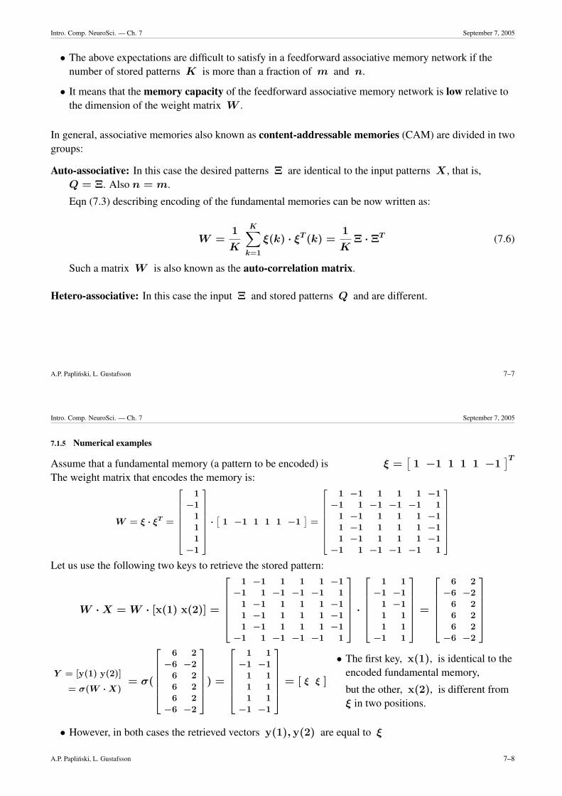
Assume that a fundamental memory (a pattern to be encoded) is ξ =[1 −1 1 1 1 −1

]T

The weight matrix that encodes the memory is:

W = ξ · ξT =

1−1

111

−1

·[

1 −1 1 1 1 −1]=

1 −1 1 1 1 −1−1 1 −1 −1 −1 1

1 −1 1 1 1 −11 −1 1 1 1 −11 −1 1 1 1 −1

−1 1 −1 −1 −1 1

Let us use the following two keys to retrieve the stored pattern:

W · X = W · [x(1) x(2)] =

1 −1 1 1 1 −1

−1 1 −1 −1 −1 11 −1 1 1 1 −11 −1 1 1 1 −11 −1 1 1 1 −1

−1 1 −1 −1 −1 1

·

1 1

−1 −11 −11 11 1

−1 1

=

6 2

−6 −26 26 26 2

−6 −2

Y = [y(1) y(2)]

= σ(W · X)= σ(

6 2

−6 −26 26 26 2

−6 −2

) =

1 1

−1 −11 11 11 1

−1 −1

= [ ξ ξ ]

• The first key, x(1), is identical to theencoded fundamental memory,

but the other, x(2), is different fromξ in two positions.

• However, in both cases the retrieved vectors y(1), y(2) are equal to ξ



7.2 Recurrent Associative Memory — Discrete Hopfield networks

• The capacity of the feedforward associative memory is relatively low, a fraction of the number ofneurons.

• When we encode many patterns often the retrieval results in a corrupted version of the fundamentalmemory.

• However, if we use again the corrupted pattern as a key, the next retrieved pattern is usually closer tothe fundamental memory.

• This feature is exploited in the recurrent associative memory networks.

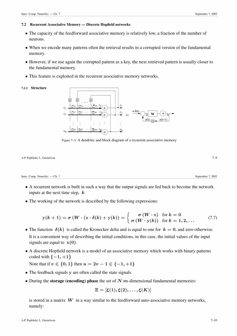
7.2.1 Structure

m

D D D

x1

x2

xm

D(k+1)(k)

δ (k).σ

σ

σ

σW m

11 w12 ww1m

2

.....

......

w21

. . .

. . .w22

...

m

y

1

y

v

...

1

2

m

y

y

y

ww2m

. . . wwmm

xv

v

.

wm2

2

mwm1

1w

Figure 7–3: A dendritic and block diagram of a recurrent associative memory



• A recurrent network is built in such a way that the output signals are fed back to become the networkinputs at the next time step, k

• The working of the network is described by the following expressions:

y(k + 1) = σ (W · (x · δ(k) + y(k)) =

{σ (W · x) for k = 0

σ (W · y(k)) for k = 1, 2, . . .(7.7)

• The function δ(k) is called the Kronecker delta and is equal to one for k = 0, and zero otherwise.

It is a convenient way of describing the initial conditions, in this case, the initial values of the inputsignals are equal to x(0).

• A discrete Hopfield network is a model of an associative memory which works with binary patternscoded with {−1, +1}Note that if v ∈ {0, 1} then u = 2v − 1 ∈ {−1, +1}

• The feedback signals y are often called the state signals.

• During the storage (encoding) phase the set of N m-dimensional fundamental memories:

Ξ = [ξ(1), ξ(2), . . . , ξ(K)]

is stored in a matrix W in a way similar to the feedforward auto-associative memory networks,namely:



W =1

m

K∑k=1

ξ(k) · ξ(k)T − K · Im =1

mΞ · ΞT − K · Im (7.8)

• By subtracting the appropriately scaled identity matrix Im the diagonal terms of the weight matrixare made equal to zero, (wjj = 0).

This is required for a stable behaviour of the Hopfield network.

• During the retrieval (decoding) phase the key vector x is imposed on the network as an initial stateof the network

y(0) = x

The network then evolves towards a stable state (also called a fixed point), such that,

y(k + 1) = y(k) = ys

It is expected that the ys will be equal to the fundamental memory ξ closest to the key x



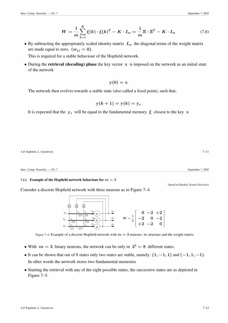
7.2.2 Example of the Hopfield network behaviour for m = 3

(based on Haykin, Neural Networks)

Consider a discrete Hopfield network with three neurons as in Figure 7–4

2/3

D

σ

σ

σ

−2/3

−2/3 −2/3

−2/3

2/3

D D

x2

x3

x1

3 yv

2

1 1y

2y2

1v

v

3

W =1

3

0 −2 +2

−2 0 −2

+2 −2 0

Figure 7–4: Example of a discrete Hopfield network with m = 3 neurons: its structure and the weight matrix

• With m = 3 binary neurons, the network can be only in 23 = 8 different states.

• It can be shown that out of 8 states only two states are stable, namely: (1, −1, 1) and (−1, 1, −1).

In other words the network stores two fundamental memories

• Starting the retrieval with any of the eight possible states, the successive states are as depicted inFigure 7–5.



(−1,−1,−1)

2

y1

y3

(y , y , y )3 2 1

(−1,−1,1)

(1,−1,−1) (1,−1,1)

(−1,1,1)

(1,1,−1) (1,1,1)

(−1,1,−1)

y

Figure 7–5: Evolution of states for two stable states

Let us calculate the network state for all possible initial states

X =

[y3

y2

y1

]=

[−1 −1 −1 −1 1 1 1 1−1 −1 1 1 −1 −1 1 1−1 1 −1 1 −1 1 −1 1

](The following MATLAB command does the trick: X = 2*(dec2bin(0:7)-’0’)’-1 )

Y = σ(W · X) =1

3

0 −2 +2

−2 0 −2

+2 −2 0

·

−1 −1 −1 −1 1 1 1 1

−1 −1 1 1 −1 −1 1 1

−1 1 −1 1 −1 1 −1 1

= σ

1

3

0 4 −4 0 0 4 −4 0

4 0 4 0 0 −4 0 −4

0 0 −4 −4 4 4 0 0

=

1 1 −1 1 1 1 −1 1

1 1 1 1 1 −1 1 −1

1 1 −1 −1 1 1 1 1



It is expected that after a number of relaxation steps

Y = W · Y

all patterns converge to one of two fundamental memories as in Figure 7–5.We will test such examples in our practical work.

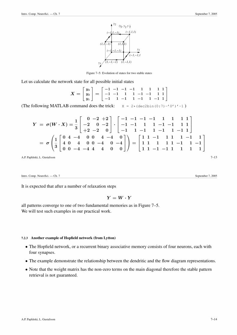
7.2.3 Another example of Hopfield network (from Lytton)

• The Hopfield network, or a recurrent binary associative memory consists of four neurons, each withfour synapses.

• The example demonstrate the relationship between the dendritic and the flow diagram representations.

• Note that the weight matrix has the non-zero terms on the main diagonal therefore the stable patternretrieval is not guaranteed.





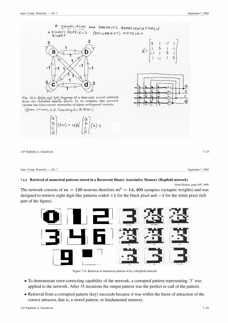
7.2.4 Retrieval of numerical patterns stored in a Recurrent Binary Associative Memory (Hopfield network)(from Haykin, pages 697, 698)

The network consists of m = 120 neurons therefore m2 = 14, 400 synapses (synaptic weights) and wasdesigned to retrieve eight digit-like patterns coded +1 for the black pixel and −1 for the white pixel (leftpart of the figure).

Figure 7–6: Retrieval of numerical patterns in by a Hopfield network

• To demonstrate error-correcting capability of the network, a corrupted pattern representing ‘3’ wasapplied to the network. After 35 iterations the output pattern was the perfect re-call of the pattern.

• Retrieval from a corrupted pattern (key) succeeds because it was within the basin of attraction of thecorrect attractor, that is, a stored pattern, or fundamental memory.



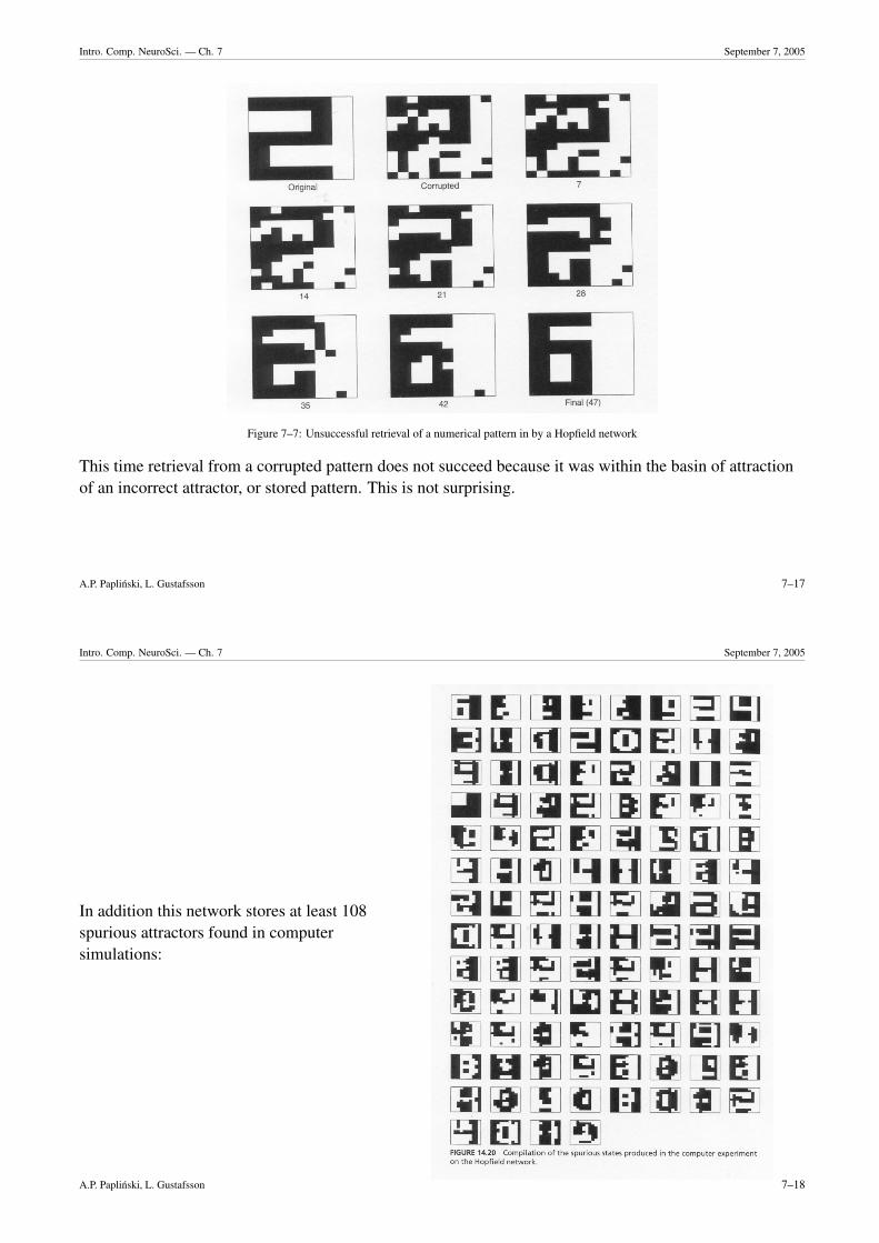
Figure 7–7: Unsuccessful retrieval of a numerical pattern in by a Hopfield network

This time retrieval from a corrupted pattern does not succeed because it was within the basin of attractionof an incorrect attractor, or stored pattern. This is not surprising.



In addition this network stores at least 108spurious attractors found in computersimulations:



• Then what does all this mean?

• It means that you cannot store memories that are similar to each other,

because if you have a slightly corrupted version of one of two similar memories,

then you can easily end up in the other one.

• It also means that even if the stored memories are not similar to each other, there will be other,spurious memories “in-between”.

• And if your corrupted initial input is closer to its own fundamental memory than to all the otherfundamental memories

it is still not certain that the proper fundamental memory will be retrieved,

it might well be a spurious attractor instead.

• The risk of retrieving the opposite of a fundamental memory is usually not great — your initial inputhas to be very corrupted for that to happen.

• All this means that the associative memory networks as we have described them are far from idealfrom a legal witness point of view.

• But their shortcomings are not unheard of from human experience.

• So their shortcomings do not rule them out as first-order models of human memory.



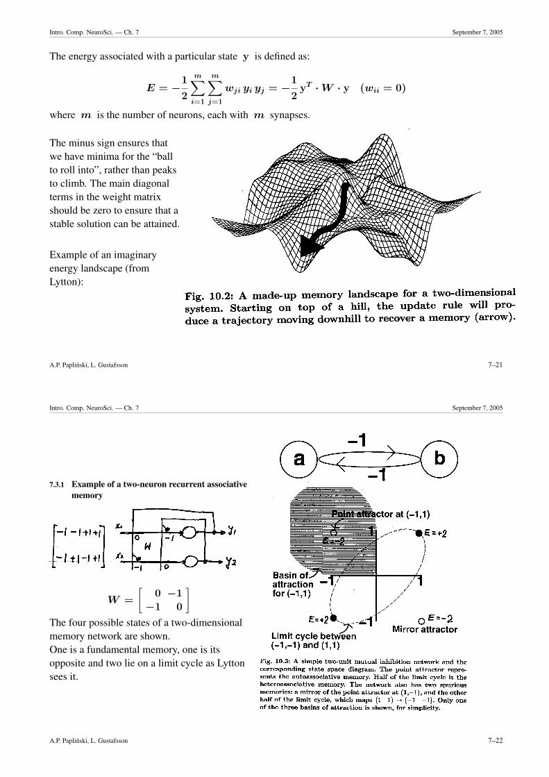
7.3 The energy landscape

• There is an “energy” associated with the states of a recurrent associative memory network.

• It is called energy because Hopfield, who used the energy concept to describe the retrieval process inan associative memory network (in the beginning of the 1980’s) is a physicist and saw the purelyformal similarity with energy functions in mechanics.

• Each attractor gives rise to a minimum, i.e. a lower point than its immediate surroundings, in thisenergy landscape.

• If the retrieval process starts from a corrupted memory, then it starts at a high energy and, like a ball ina real landscape, it rolls down to a minimum, hopefully to the right one.

• A problem is that the ball rolls in a high-dimensional landscape, which makes it difficult to illustrateon paper.

• The energy of the spurious attractors is generally higher than the energy of the fundamental memories,so if you can “feel this energy” then you have a chance to say that what you seem to remember mightbe wrong.

• The opposite attractors of the fundamental memories have the same low energies as the attractorsthemselves so in this case you are left without assistance.



The energy associated with a particular state y is defined as:

E = −1

2

m∑i=1

m∑j=1

wji yi yj = −1

2yT · W · y (wii = 0)

where m is the number of neurons, each with m synapses.

The minus sign ensures thatwe have minima for the “ballto roll into”, rather than peaksto climb. The main diagonalterms in the weight matrixshould be zero to ensure that astable solution can be attained.

Example of an imaginaryenergy landscape (fromLytton):



7.3.1 Example of a two-neuron recurrent associativememory

W =

[0 −1

−1 0

]The four possible states of a two-dimensionalmemory network are shown.One is a fundamental memory, one is itsopposite and two lie on a limit cycle as Lyttonsees it.


Lennart Gustafsson page

Course notes CSE2330

19

Chapter 10 Associative Memory Networks

A higher dimensional example

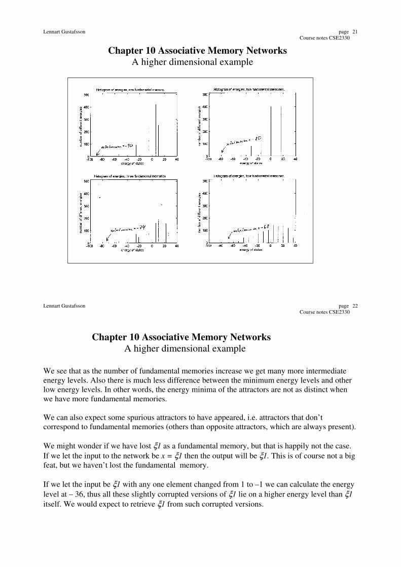
Let us study an example. We begin by storing one vector as a fundamental memory. The

particular choice of vector is not important , let us choose ξ1 = [1 1 1 1 1 1 1 1 1 1]'.

The energy minimum has two minima at E = -90, one for x = [1 1 1 1 1 1 1 1 1 1]'

and one for x = [-1 -1 -1 -1 -1 -1 -1 -1 -1 -1]', just as was stated before.

There are several more energy levels, but the levels are discrete since the elements can only

assume the values 1 and –1.

If we store two vectors, ξ1 = [1 1 1 1 1 1 1 1 1 1]' and ξ2 = [1 1 1 1 1 -1 -1 -1 -1 -1]', then as

expected we have minima at E = -80 for ξ1 and ξ2 and their “opposites”.



20



If we store three vectors, ξ1 = [1 1 1 1 1 1 1 1 1 1]' and ξ2 = [1 1 1 1 1 -1 -1 -1 -1 -1]' and

ξ3=[1 -1 1 -1 1 -1 1 -1 1 -1]', then we have minima at E = -74 but only at ξ2 and ξ3.

The energy at ξ1 is slightly higher, at –70.

If we store four vectors, ξ1 = [1 1 1 1 1 1 1 1 1 1]' and ξ2 = [1 1 1 1 1 -1 -1 -1 -1 -1]',

ξ3 = [1 -1 1 -1 1 -1 1 -1 1 -1]' and ξ4 = [1 1 -1 -1 1 1 -1 -1 -1 1]', then we have minima

at E = -68 but only at ξ2, ξ3 and ξ4. Again the energy at ξ1 is slightly higher, at –60.

There are more differences between are four cases which become clear when we study the

histograms for the energies. Let us do that.



21





22



We see that as the number of fundamental memories increase we get many more intermediate

energy levels. Also there is much less difference between the minimum energy levels and other

low energy levels. In other words, the energy minima of the attractors are not as distinct when

we have more fundamental memories.

We can also expect some spurious attractors to have appeared, i.e. attractors that don’t

correspond to fundamental memories (others than opposite attractors, which are always present).

We might wonder if we have lost ξ1 as a fundamental memory, but that is happily not the case.

If we let the input to the network be x = ξ1 then the output will be ξ1. This is of course not a big

feat, but we haven’t lost the fundamental memory.

If we let the input be ξ1 with any one element changed from 1 to –1 we can calculate the energy

level at – 36, thus all these slightly corrupted versions of ξ1 lie on a higher energy level than ξ1

itself. We would expect to retrieve ξ1 from such corrupted versions.

7 associative memory networks related to/based on...

Documents