7 more one-sample con dence intervals and tests, part 1 of...

7 More One-Sample Confidence Intervals and Tests, Part 1 of 2

We already have a Z confidence interval (§5) and a Z test (§6) for an unknown mean µ for whenwe know σ and have a normal population or large n. In this unit we study:

• the Student’s tn−1 distribution of T = X̄−µS/√n

, useful with (compare T to Z =

X̄−µσ/√n

); and a T CI and test for µ for a normal population or large n and an unknown σ

• the relationship between a two-sided confidence interval and a

• power = P (reject H0| )

• a bootstrap CI and test for µ requiring only a simple random sample

• a sign test for an unknown M requiring only a simple random sample

• a Z CI and test for an unknown proportion π

• extra examples (if time allows)

1

The Student’s t Distribution

Now suppose we have a normal X̄ ∼ N(µ, σ2/n) are interested in µ but don’t know σ. Define the

random variable T = X̄−µS/√n

. T ’s distribution isn’t normal; it’s the Student’s t distribution with n−1

degrees of freedom, denoted tn−1. (“Student” is a pseudonym for William Gosset, a statistician at.)

• Properties of T ∼ tn−1:

– T is a sample version of a , estimating how far X̄ is from ,in

– tn−1 looks like N(0, 1): symmetric about , -peaked, and -shaped

– T ’s variance is than Z’s because estimating σ ( ) by S ( )gives T more variation than Z: tn−1 is shorter with thicker tails (draw N(0, 1) and t6−1)

– As n increases, tn−1 gets closer to (S becomes aof σ); in the limit as n→∞, they’re

• t table:

Let tn−1,α = the critical value t cutting off a area of α from tn−1

(draw). The posted Student’s t table gives tail probabilities.

HH

HHH

H

HHH

HHH

T ∼ tn−1

0

α = shaded area

tn−1,α

e.g. Use the t table to find the critical value t

– cutting off a right tail area of .05 from the t6−1 distribution: t5,.05 =

– such that the area under the t22−1 curve between −t and t is 98%

– such that the area under the t25−1 curve left of t is .025

2

Confidence interval using the Student’s t distribution

Theorem:

If X1, . . . , Xn is a simple random sample, from N(µ, σ2) or where n is large (say n > 30), thenX̄ ± tn−1,α/2

S√n

contains µ for a proportion 1− α of random samples.

Proof:

e.g. Recall §5 example with a warehouse of thousands of painted engine blocks; a random 16 havepaint thickness measured, with x̄ = 1.348 and s = .339. Make a 95% confidence interval for µ, theunknown population mean thickness (supposing now we don’t know σ).

n = ; Is n large enough or is sample from normal population? Try qqnorm(paint):Histogram of Paint Thickness

paint thickness (mil)

Den

sity

0.8 1.2 1.6 2.0

0.0

0.6

1.2

●

●

●

●

●●

●

●

●

●

●

●

●

●

●

●

−2 −1 0 1 2

0.8

1.2

1.6

QQ Plot of Paint Thickness

Theoretical Quantiles

Sam

ple

Qua

ntile

s

We have 1−α = =⇒ α = =⇒ tn−1,α/2 = ,

so x̄± tn−1,α/2s√n

=

With what probability does our interval contain µ?

e.g. In a sample of 100 boxes of a certain type, the average compressive strength was 6230 N, andthe standard deviation was 221 N.

a. Find a 95% confidence interval for the mean compressive strength.

b. Find a 99% confidence interval for the mean compressive strength.

3

Hypothesis test using the Student’s t distribution

Now suppose an engine design specification says the paint thickness should be 1.50 mil. We wantto know whether the device is off this mark on average, so that it should be re-calibrated to correctits population mean thickness, µ.

We test the hypothesis H0 : against HA : .

If the population is normal or n is large enough that the CLT applies, and if H0 is true, thenX̄ ∼ N(µ0,

σ2

n )(≈), where µ0 is the value of µ under

H0 : X̄ ∼ N(µ0, σ2/n)

µ0

That means T =X̄ − µ0

S/√n∼ tn−1:

T ∼ tn−1

0

Values of X̄ far from µ0 (in ), or equivalently, values of t far fromindicate strong evidence against H0.

Let’s use significance level α = .05. We have three options for completing the test.

4

• Find the rejection region corresponding to a chosen significance level α = P (type I error) =. This region is T < −tn−1,α/2 or T > tn−1,α/2

(draw). Compute t and reject H0 if it is in the region.

For the paint, we have n = 16, so we need t16−1,0.025 = . Our rejectionregion is . Our observed t is

tobs =x̄− µ0

s/√n

=

Conclusion:

• Compute the p-value and compare it to α.

We have tobs = −1.796, so our p-value is (draw)

p-value = P (T is as extreme or more extreme than tobs|H0 is true) =

– from the t table, , or

– from R, use 2 * pt(q = -1.796, df=15) =

Conclusion:

• Compute a confidence interval and check whether µ0 is in it (below).

5

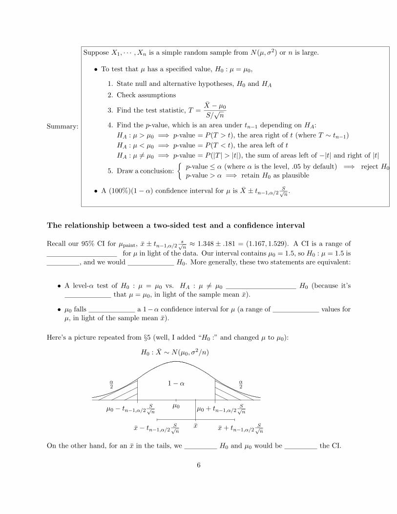
Summary:

Suppose X1, · · · , Xn is a simple random sample from N(µ, σ2) or n is large.

• To test that µ has a specified value, H0 : µ = µ0,

1. State null and alternative hypotheses, H0 and HA

2. Check assumptions

3. Find the test statistic, T =X̄ − µ0

S/√n

4. Find the p-value, which is an area under tn−1 depending on HA:

HA : µ > µ0 =⇒ p-value = P (T > t), the area right of t (where T ∼ tn−1)

HA : µ < µ0 =⇒ p-value = P (T < t), the area left of t

HA : µ 6= µ0 =⇒ p-value = P (|T | > |t|), the sum of areas left of −|t| and right of |t|

5. Draw a conclusion:

{p-value ≤ α (where α is the level, .05 by default) =⇒ reject H0

p-value > α =⇒ retain H0 as plausible

• A (100%)(1− α) confidence interval for µ is X̄ ± tn−1,α/2S√n

.

The relationship between a two-sided test and a confidence interval

Recall our 95% CI for µpaint, x̄ ± tn−1,α/2s√n≈ 1.348 ± .181 = (1.167, 1.529). A CI is a range of

for µ in light of the data. Our interval contains µ0 = 1.5, so H0 : µ = 1.5 is, and we would H0. More generally, these two statements are equivalent:

• A level-α test of H0 : µ = µ0 vs. HA : µ 6= µ0 H0 (because it’sthat µ = µ0, in light of the sample mean x̄).

• µ0 falls a 1−α confidence interval for µ (a range of values forµ, in light of the sample mean x̄).

Here’s a picture repeated from §5 (well, I added “H0 :” and changed µ to µ0):

��

��

��

HH HHHH

HHHH

HH

µ0 − tn−1,α/2S√n

H0 : X̄ ∼ N(µ0, σ2/n)

µ0

α2

1− α α2

µ0 + tn−1,α/2S√n

x̄x̄− tn−1,α/2S√n

x̄+ tn−1,α/2S√n

On the other hand, for an x̄ in the tails, we H0 and µ0 would be the CI.

6

e.g. Two-sided CI vs. test

1. A researcher interested in the aluminum recycling market collects 20 cans that he regards asa simple random sample from the local population of cans. He finds a 99% confidence intervalfor µ, the population mean weight of cans, as 14.2± .05 g.

(a) What decision should he make about H0 : µ = 14.3 vs. HA : µ 6= 14.3?

(b) What decision should he make about H0 : µ = 14.22 vs. HA : µ 6= 14.22?

2. The P -value for a two-sided test of H0 : µ = 10 vs. HA : µ 6= 10 is 0.06.

(a) Does the 95% confidence interval for µ include 10? Why?

(b) Does the 90% confidence interval for µ include 10? Why?

7

Power (for the known-σ case)

Recall:

• β = P (type error) = P (do not reject H0|H0 is false)

• power = 1− β = P (reject H0|H0 is false)

Neither is well-defined until we choose a particular value, , in the region specified by HA.

e.g. For the paint test of H0 : µ = 1.5 vs. HA : µ 6= 1.5, suppose we know σpaint thickness = 0.30 mil.Find powerµA=1.4.

1. Use H0 : µ = 1.5 and α = .05 to find the rejection region: .

By unstandardizing from Z = X̄−µ0σ/√n

, find the equivalent rejection region in X̄ as

X̄ < or X̄ > (draw)

1.2 1.3 1.4 1.5 1.6 1.7 1.8

X ~ N(µ, (σ n)2) for two values of µ

µ0 = 1.5µA = 1.4

µ0µA

2. Now use the particular HA value µA to find powerµA=1.4 =

This power is : if the true mean were µ = 1.4, we would probablyH0 based on a sample of size 16, even though H0 is .

8

To increase power,

• |µ0 − µA|

• the type-I error rate, α

• the sample size, n

• the population standard deviation, σ

Here we find formulas to do similar power calculations more generally.

• For a one-sided test, HA : µ < µ0 (or HA : µ > µ0), power =


µ0µA

µ0µA

• For a two-sided test, HA : µ 6= µ0 power =


µ0µA

µ0µA

Power of a test of H0 : µ = µ0 when H0 is false because µ = µA:

• For a one-sided test, HA : µ < µ0 or HA : µ > µ0, powerµA = P

(Z <

|µ0 − µA|σ/√n− zα

).

• For a two-sided test, HA : µ 6= µ0, powerµA ≈ P(Z <

|µ0 − µA|σ/√n− zα/2

).

e.g. Check that the formula give the same power for the paint test as we found earlier.

9

Power and sample size

Now we find the sample size n required to achieve power 1 − β to reject H0 at level α when aparticular HA is true:

Z =X − µ0

σ n~ N(0, 1); rejection region for level α uses zα 2

0− zα 2 zα 2

Z =X − µA

σ n~ N(0, 1); power 1 − β uses zβ

0 zβ

X ~ N(µ, (σ n)2) for two values of µ; set X−zα 2= Xzβ and solve for n

µ0µA

For a test of H0 : µ = µ0 vs. HA : µ 6= µ0 at level α, the sample size n required to have power 1−β

when the true µ is µA is n ≈(σ(zα/2 + zβ)

µ0 − µA

)2

.

e.g. For the paint, suppose σ = 0.30 is known, and we seek the sample size n required to have power0.8 to reject H0 at level α = .05 when the true mean is µA = 1.4. We need n =

10

7 More One-Sample Confidence Intervals and Tests, Part 2 of 2

Bootstrap for a confidence interval or test for µ

So far, our discussion of estimating the population mean µ has assumed either the population isnormal, so that X̄ is also , or the sample size is for theCLT to indicate that X̄ is approximately normal. What if neither is true?

e.g. Secondhand smoke presents health risks, especially to children. A SRS was taken of 15 childrenexposed to secondhand smoke, and the amount of cotanine (a metabolite of nicotine) in their urinewas measured. The data were: 29, 30, 53, 75, 34, 21, 12, 58, 117, 119, 115, 134, 253, 289, 287. Arethese data strong evidence cotanine is above 75 units in kids exposed to secondhand smoke? (It isbelow 75 in unexposed kids.)

First, check graphs to see whether an assumption of a normal population is :

Secondhand smoke and children(histogram and density plot)

Cotanine level

Den

sity

0 50 150 250

0.00

00.

004

● ●●

●

●●●

●

● ●●●

●

●●

−1 0 1

5015

030

0

QQ Plot for Cotanine Data


Sam

ple

Qua

ntile

s

This looks pretty bad, so we worry about a normality assumption. The sample is small, so theCLT may not help. Without a normal X̄, the quantity

T = X̄−µS/√n

will not have a distribution. The bootstrap is a sneaky way to estimatethe true distribution of this T . It estimates the of a statisticby sampling with replacement from a simple random sample from a popluation. e.g. Here’s ahand-waving account . . .

11

To use the bootstrap to make a confidence interval or do a hypothesis test for a mean µ,

1. Collect one simple random sample of size n from the population. Compute the sample mean,x̄ (an estimate of the population mean, µ) and the sample standard deviation, s (an estimateof the population standard deviation, σ).

2. Draw a random sample of size n, , from the data. Callthese observations x∗1, x∗2, ..., x∗n. Some data may appear more than once in this resampling,and some not at all.

3. Compute the and of the resampled data. Call these x̄∗ and s∗.

4. Compute the statistic t̂ =x̄∗ − x̄s∗/√n

5. Repeat steps 2-4 a large number of times, accumulating many t̂’s. They approximate the

(unknown) sampling distribution of T = X̄−µS/√n

.

6. To find a (100%)(1 − α) confidence interval for µ, find the 1 − α/2 and α/2 upper criticalvalues of the approximate sampling distribution, calling them t̂(1−α/2) and t̂(α/2). The

bootstrap 100(1− α)% confidence interval is

(x̄− t̂(α/2)

s√n, x̄− t̂(1−α/2)

s√n

).

7. To test H0 : µ = µ0, compute tobs = x̄−µ0s/√n

. Find the p-value, an area under the approximate

sampling distribution density curve given by , where m depends on HA:

HA : µ > µ0 =⇒ m is the number of values of t̂ for which t̂ tobs

HA : µ < µ0 =⇒ m is the number of values of t̂ for which t̂ < tobs

HA : µ µ0 =⇒ m is the number of values of t̂ for which t̂ < −|tobs| or t̂ > |tobs|

Draw a conclusion as usual:



12

e.g. For the secondhand smoke data, we find x̄ = 108.4 and s = 95.6. Bootstrapping 5000 timesyields the following approximate distribution of t (draw for interval on left and for test on right):

Approximate Sampling Distribution of T

Bootstrap t̂ values

Den

sity

−10 −5 0 5

0.00

0.05

0.10

0.15

0.20

0.25

0.30

0.35

Approximate Sampling Distribution of T

Bootstrap t̂ values

Den

sity

−10 −5 0 5

0.00

0.05

0.10

0.15

0.20

0.25

0.30

0.35

Unlike a t or normal distribution, this distribution is symmetric.

Make a bootstrap confidence interval for µ = population mean cotanine in smoky kids

The upper critical values, from R, are t̂(1−α/2) = −3.56 and t̂α/2 = 1.86 (draw, above left), so theinterval is(

108.4− ( ) 95.6√15, 108.4− ( ) 95.6√

15

)≈ (62.5, 196.3).

This interval is not symmetric about x̄. It would on bootstrapping again.

Run a bootstrap test for µ

We wish to know whether µ is greater than 75, so we test H0 : µ = 75 vs. HA : .

Find tobs = .

Draw the p-value, above right.

Here (from R) m = 348 of the bootstrap values were greater than 1.353, so the p-value is, and, at level α = .05, we would H0.

13

Here is one way to do this bootstrap using R:

# Create a new function, bootstrap(x, n.boot), having two inputs:

# - x is a data vector

# - n.boot is the desired number of resamples from x

# It returns a vector of n.boot t-hat values.

bootstrap = function(x, n.boot) {

n = length(x)

x.bar = mean(x)

t.hat = numeric(n.boot) # create vector of length n.boot zeros

for(i in 1:n.boot) {

x.star = sample(x, size=n, replace=TRUE)

x.bar.star = mean(x.star)

s.star = sd(x.star)

t.hat[i] = (x.bar.star - x.bar) / (s.star / sqrt(n))

}

return(t.hat)

}

# Use the bootstrap() function to get an approximate sampling

# distribution of T for the smoke data.

data = c(29, 30, 53, 75, 34, 21, 12, 58, 117, 119, 115, 134, 253, 289, 287)

B = 5000

t.hats = bootstrap(data, B)

# Plot the approximate sampling distribution.

hist(t.hats, freq=FALSE, xlab = "Bootstrap t-hat values",

main = "Approximate Sampling Distribution of T")

n = length(data) # Get summary statistics.

x.bar = mean(data)

s = sd(data)

cat(sep="", "n=", n, ", x.bar=", x.bar, ", s=", s, "\n")

# Make a CI for mu. First find quantiles for a 95% interval.

t.lower = quantile(t.hats, probs=.025) # This is our t_{1 - alpha.2}.

t.upper = quantile(t.hats, probs=.975) # This is our t_{alpha/2}.

cat(sep="", "t.lower=", t.lower, ", t.upper=", t.upper, "\n")

ci.low = x.bar - t.upper * s / sqrt(n) # This is our lower interval endpoint.

ci.high = x.bar - t.lower * s / sqrt(n) # This is our upper interval endpoint.

cat(sep="", "confidence interval: (", ci.low, ", ", ci.high, ")\n")

# Run a test of H_0: mu = m_0. First find t_{obs}.

mu.0 = 75

t.obs = (x.bar - mu.0) / (s / sqrt(n))

14

cat(sep="", "t.obs=", t.obs, "\n")

# sum() counts the TRUE values by first converting TRUE / FALSE values to 1 / 0.

m.left = sum(t.hats < t.obs) # This is for H_A: mu < mu_0.

p.value.left = m.left / B

cat(sep="", "m.left=", m.left, ", B=", B, ", p.value.left=", p.value.left, "\n")

m.right = sum(t.hats > t.obs) # This is for H_A: mu > mu_0.

p.value.right = m.right / B

cat(sep="", "m.right=", m.right, ", B=", B, ", p.value.right=", p.value.right, "\n")

# This is for H_A: mu != mu_0. ("!=" means "is not equal to.")

m.left.abs = sum(t.hats < -abs(t.obs))

m.right.abs = sum(t.hats > abs(t.obs))

p.value.two.sided = (m.left.abs + m.right.abs) / B

cat(sep="", "m.left.abs=", m.left.abs, ", m.right.abs=", m.right.abs,

", B=", B, ", p.value.two.sided=", p.value.two.sided, "\n")

15

Sign test for an unknown median M

If the data do not seem to be from a normal population and the sample size is small, an alternativeto the bootstrap is the sign test. It is a test for a . If the population is roughly

, the sign test is equivalent to a test for a .

e.g. A city trash department is considering separating recyclables from trash to save landfill spaceand sell the recyclables. Based on data from other cities, if more than half the city’s householdsproduce 6 lbs or more of recyclable material per collection period, the separation will be profitable.A random sample of 11 households yields these data on material per household in pounds:

14.2, 5.3, 2.9, 4.2, 1.8, 6.3, 1.1, 2.6, 6.7, 7.8, 25.9

We start with plotting. Here are a histogram and QQ plot:

Histogram Recyclable Material

Recyclable Material (pounds)

Fre

quen

cy

0 5 10 15 20 25 30

01

23

45 M0 = 6

●

●

●●

●

●

●●

●●

●

−1.5 −0.5 0.5 1.0 1.5

510

1520

25

QQ Plot of Recyclable Material


Sam

ple

Qua

ntile

s

Neither plot suggests a normal population: both show . Since we have n = 11,the CLT is , and, in any case, our question is really about a . So, lettingM be the population , we test:

H0 : M = 6HA :

We need a test statistic. If H0 is true, the sample should have about of theobservations greater than 6 and less than 6. The probability of observing a valuegreater than 6 in the sample should be . A natural choice of test statistic is the number, B,

16

of observations greater than 6. Under H0, B ∼ . (Note: n is the numberof observations the null value of the median. If any of the observations wereequal to 6, we would .)

The value of the test statistic is b =

(Equivalently, this is the number of positive differences from M0. These differences are:

, ,−3.1,−1.8,−4.2, 0.3,−4.9,−3.4, 0.7, 1.8,

Of these differences, are positive. The sign test counts the number of “+” signs.)

The p-value is

R can find this p-value via sum(dbinom(x=5:11, size=11, prob=.5)).

Our conclusion is:

For a two-sided test, find P (B ≥ b) and P (B ≤ b) and use .

Summary:

Suppose X1, . . . , Xn is a simple random sample from a population with median M . To test thatM has a specified value, M0,

0. (First discard any data equal to M0, reducing n accordingly.)

1. State null and alternative hypotheses, H0 : M = M0 and HA


3. Find differences from the median, X1−M0, . . . , Xn−M0, and the test statistic, B = numberof positive differences

4. Find the p-value, which is a probability for B ∼ Bin(n, .5) depending on HA:

HA : M > M0 =⇒ p-value = P (B ≥ b)HA : M < M0 =⇒ p-value = P (B ≤ b)HA : M 6= M0 =⇒ p-value = 2×min

[P (B ≤ b), P (B ≥ b), 1

2

]5. Draw a conclusion:



17

Estimation of an unknown population proportion π

e.g. An accounting firm has a large list of clients (the population), with an information file on eachclient. The firm has noticed errors in some files and wishes to know the proportion of files thatcontain an error. Call the population proportion of files in error π. An SRS of size n = 50 is takenand used to estimate π. Now the firm will decide whether it is worth the cost to examine and fixall the files. Each file sampled was classified as containing an error (call this 1), or not (call this0). The results are:

Files with an error: 10; files without errors, 40.

To develop an estimator of π, recall the binomial distribution: X ∼ Bin(n, π) is thein independent trials, each having possible outcomes (success and fail-ure), and each having probability of success. We found E(X) = , V AR(X) =

.

Our estimator of the population proportion is the sample proportion P = Here are some of itsproperties:

• E(P ) =

• V AR(P ) =

• SD(P ) =

√π(1−π)

n

This tells us our estimator P is for π, and gives a measure of precision. As in thediscussion of X̄, we can estimate the standard deviation by plugging in our estimator of π:

To make a confidence interval or do a test for π, we need the distribution of P . Its exact distributionis related to the binomial distribution, which is difficult to use in this context. However, the CLTcan help. If n is large enough, the conditions of the CLT are met, because X =

∑Yi (where Yi is

a Bernoulli trial, either 0 or 1), so P = Xn = 1

n

∑Yi is a . . Thus, for large

samples, P is approximately distributed:

P ∼ N

(π,

[√π(1−π)

n

]2)

(≈)

We want to use this distribution to make a confidence interval for π and do a test on π, but we

don’t know π, so we have to estimate the standard deviation,

√π(1−π)

n .

18

• For the interval, use the sample proportion P to estimate π, so the standard deviation of P

is about SP =

√P (1−P )

n . A rule of thumb says we numbers of successes and failures,and , each to be greater than 5 for the CLT approximation to be reasonable.

The 100%(1− α) confidence interval for π is then P ± zα/2√

P (1−P )n .

Proof:

e.g. Find a 95% CI for the unknown proportion π of defective files.

• The test comes with a null hypothesis, H0 : π = π0, so we should use π0 for π in the

standard deviation of P and say, if H0 is true, then P ∼ N

(π,

[√π0(1−π0)

n

]2)

(≈). A rule

of thumb says we need the expected numbers of successes and failures, and ,each to be greater than 5 for the CLT approximation to be reasonable. Standardizing givesZ = P−π0√

π0(1−π0)n

∼ N(0, 1), which we can use as a test statistic.

e.g. The CEO decides that if π > .12, it will be worthwhile to review and fix every file. Runa test to help the CEO decide.

We test: H0 : π = (π0 = 0.12) vs. HA : .

In our example we have nπ0 = and n(1−π0) = .

We observed zobs =

Our p-value =

Our conclusion is

19

Summary:

Let X be the number of successes in a large number n of independent Bernoulli trials, each havingprobability π of success. Let P = X

n .

• To test that π has a specified value, π0, where nπ0 > 5 and n(1− π0) > 5,

1. State null and alternative hypotheses, H0 : π = π0 and HA


3. Find the test statistic Z =P − π0√

π0(1− π0)/n

4. Find the p-value, which depends on HA:

HA : π > π0 =⇒ p-value = P (Z > z), the area right of z

HA : π < π0 =⇒ p-value = P (Z < z), the area left of z

HA : π 6= π0 =⇒ p-value = P (|Z| > |z|), the sum of the ares left of −|z| and right of |z|

5. Draw a conclusion:



• An approximate 100%(1− α) confidence interval for π is P ± zα/2√

P (1−P )n , provided X > 5

and n−X > 5.

Demonstrate that P ∼ N(. . .)

Our CI and test for π relied on the CLT to say P = Xn ∼ N(. . .)(≈) because P is a sample mean.

X is a sample sum, which is also N(. . .). In particular, X ∼ Bin(n, π) ≈ N(nπ, nπ(1− π)).

Here is a graphical comparison of Bin(n, π) with N(nπ, nπ(1−pi)) for n = 20 and several values of πto help with understanding the CLT claim and our rule-of-thumb requiring nπ > 5 and n(1−π) > 5.(You may ignore the code. I’ll run it and discuss it.)

n=20

delta.p=.1

for (p in seq(from=delta.p, to=1-delta.p, by=delta.p)) {

Sys.sleep(3)

y=dbinom(x=0:n, size=n, prob=p)

curve(dnorm(x, mean=n*p, sd=sqrt(n*p*(1-p))), 0, n, ylab="",

main=bquote("n=" * .(n) * ", " * pi * "=" * .(p) *

", " * n * pi * "=" * .(n*p) * ", " * n * (1- pi) *

"=" * .(n*(1-p))))

segments(x0=0:n, y0=0, y1=y)

}

In §8, we compare populations via independent samples.

20

Extra examples (if time allows)

Extra confidence intervals for µ with known or unknown σ

The basal diameter of a sea anemone indicates its age. Suppose the population mean (µ) andstandard deviation (σ) are unknown.

1. Here are the diameters of a simple random sample of 40 anemones: 4.3, 5.7, 3.9, 4.8, 3.5, 3.5,1.3, 4.6, 4.4, 3.7, 4.9, 5.6, 5.1, 2.3, 2.3, 6.9, 5.4, 3.6, 4.3, 4.1, 3.2, 4.6, 2.8, 4.9, 4.5, 4.4, 5.8, 3.6,5.6, 2.6, 1.5, 4.1, 4.7, 6.5, 5.4, 3.8, 3.4, 4.9, 5.5, 7.2. These data have x̄ = 4.33 and s = 1.329.Find a 95% confidence interval for µ or explain why you cannot.

2. Here is a simple random sample of 12 anemone diameters: 5.3, 2.8, 5.2, 2.9, 2.5, 2.9, 3.0, 2.9,5.2, 4.3, 3.7, 2.7. Find a 95% confidence interval for µ or explain why you cannot.

3. Here is a simple random sample of 12 anemone diameters: 3.5, 6.5, 3.6, 2.8, 4.2, 4.2, 1.8, 5.7,2.6, 4.7, 4.9, 4.4. Find a 95% confidence interval for µ or explain why you cannot.

4. (Inference) Now suppose the population mean (µ) is unknown but σ = 1.4 cm is known.What changes in the intervals above?

21

Extra bootstrap sanity check

• Bootstrap confidence interval for an unknown mean

Let’s do “sanity check” computer simulations to see whether the bootstrap does somethingreasonable when we know what to expect. Suppose X1, . . . , Xn is a SRS from N(0, 12), a

normal population. In this case, we know that T = X̄−µS/√n∼ tn−1.

– Do a bootstrap to get an approximate sampling distribution (labeled “Resampling dis-tribution of T” in the graphs) for T and see whether it looks like tn−1.

– How do the results depend on n?

∗ Resampling with replacement from a large sample seems like a good approximationto repeated sampling from the population.

∗ Resampling with replacement from a small sample seems like a lousy approximationto repeated sampling from the population.

−3 −2 −1 0 1 2 3

0.0

0.1

0.2

0.3

0.4

(Bootstraph sanity check: Will we get tn−1?) N(0, 1) Population and SRS of size n=100

x

●

−3 −2 −1 0 1 2 3

01

23

4

Sample means: N(0, (1 n)2)

vertical lines cut off 95% of distributionx

Theoretical N(0, (1/sqrt(n))^2)bootstrap x.bars

−3 −2 −1 0 1 2 3

0.0

0.1

0.2

0.3

0.4

Resampling distribution of T


theoretical tn−1bootstrap t's

22

−3 −2 −1 0 1 2 3

0.0

0.1

0.2

0.3

0.4


x

●

−3 −2 −1 0 1 2 3

0.0

0.4

0.8

1.2




−3 −2 −1 0 1 2 3

0.0

0.1

0.2

0.3

0.4




−3 −2 −1 0 1 2 3

0.0

0.1

0.2

0.3

0.4


x

●

−3 −2 −1 0 1 2 3

0.0

0.4

0.8




−3 −2 −1 0 1 2 3

0.05

0.20

0.35




23

Extra sign test for M

e.g. A clinical trial measured survival time in weeks for 10 lymphoma patients as 49, 58, 75, 110,112, 132, 151, 276, 281, 362+, where “+” indicates a patient still alive at the end of the study.Are these data strong evidence the population median survival time M for lymphoma patients isis different than 200?

Extra inference for one proportion π

e.g. Monica learned in first grade that about 71% of Earth’s surface is covered in water. To seewhether this made sense, she asked her brother to toss her a spinning inflatable globe 100 times.For 66 of her catches, her right pointer finger tip was on water, while for 34 it was on land. Nowshe’s stuck. Help her by finding and interpreting a 99% confidence interval for the proportion ofEarth covered by water in light of her data.

e.g. Do children prefer vanilla or chocolate ice cream? To test this, a teacher gave a random sampleof 33 students the choice. 24 of 33 chose chocolate, and the other 9 chose vanilla. Use these datato test the hypothesis that, in the population, students have no preference.

24

7 more one-sample con dence intervals and tests, part 1 of...

Documents