7 nonparametric methods

7 NONPARAMETRIC METHODS

7 Nonparametric Methods

SW Section 7.11 and 9.4-9.5

Nonparametric methods do not require the normality assumption of classical techniques. Iwill describe and illustrate selected non-parametric methods, and compare them with classicalmethods. Some motivation and discussion of the strengths and weaknesses of non-parametricmethods is given.

The Sign Test and CI for a Population Median

The sign test assumes that you have a random sample from a population, but makes no assumptionabout the population shape. The standard t−test provides inferences on a population mean. Thesign test, in contrast, provides inferences about a population median.

If the population frequency curve is symmetric (see below), then the population median, iden-tified by η, and the population mean µ are identical. In this case the sign procedures provideinferences for the population mean.

The idea behind the sign test is straightforward. Suppose you have a sample of size m fromthe population, and you wish to test H0 : η = η0 (a given value). Let S be the number of sampledobservations above η0. If H0 is true, you expect S to be approximately one-half the sample size,.5m. If S is much greater than .5m, the data suggests that η > η0. If S is much less than .5m, thedata suggests that η < η0.

Mean = µMedian = η

50%

Mean and Median differ with skewed distributions

Mean = Median

Mean and Median are the same with symmetric distributions

S has a Binomial distribution when H0 is true. The Binomial distribution is used to constructa test with size α (approximately). For a two-sided alternative HA : η 6= η0, the test rejects H0

when S is significantly different from .5m, as determined from the reference Binomial distribution.One sided tests use the corresponding lower or upper tail of the distribution. To generate a CI forη, you can exploit the duality between CI and tests. A 100(1 − α)% CI for η consists of all valuesη0 not rejected by a two-sided size alpha test of H0 : η = η0.

83


Comments:

1. Minitab omits all observations at exactly η0, so m is the sample size after omissions. Thisshould not be much of a concern unless the measurements are coarsely rounded.

2. Not all test sizes and confidence levels are possible because the test statistic S is discretevalued. Minitab gives an exact p-value for the test, and approximates the desired confidencelevel using a non-linear interpolation algorithm.

3. To implement the sign procedures in Minitab follow: Stat > Nonparametrics > 1-SampleSign. The dialog box allows you to specify a test or a CI, but not both at the same time.The tests can be two-sided or one-sided.

4. Only two-sided CIs are available, so you have to be clever to get a one-sided bound. For ex-ample, to get an upper 95% bound, you take the upper limit from a 90% two-sided confidenceinterval. The rational for this is that with the 90% two-sided CI, the population parameterwill fall above the upper limit 5% of the time and fall below the lower limit 5% of the time.Thus, you are 95% confident that the population parameter falls below the upper limit of thisinterval, which gives us our one-sided bound. The same logic applies if you want to generalizethe one-sided confidence bounds to arbitrary confidence levels and to lower one-sided bounds- always double the error rate of the desired one-sided bound to get the error rate of therequired two-sided interval! For example, if you want a lower 99% bound (with a 1% errorrate), use the lower limit on the 98% two-sided CI (which has a 2% error rate).

Example: Income Data

Recall that the income distribution is extremely skewed, with two extreme outliers at 46 and1110. The presence of the outliers has a dramatic effect on the 95% CI for the population meanincome µ, which goes from -101 to 303 (in 1000 dollar units). This t−CI is suspect because thenormality assumption is unreasonable. A CI for the population median income η is more sensiblebecause the median is likely to be a more reasonable measure of typical value. Using the signprocedure, you are 95% confident that the population median income is between 2.79 and 10.95(times 1000 dollars).

Data Display

Income7 1110 7 5 8 12 0 5 2 2 467

One-Sample T: Income

Variable N Mean StDev SE Mean 95% CIIncome 12 100.917 318.008 91.801 (-101.136, 302.969)

Sign CI: Income

84


Sign confidence interval for median

ConfidenceAchieved Interval

N Median Confidence Lower Upper PositionIncome 12 7.00 0.8540 5.00 8.00 4

0.9500 2.79 10.95 NLI0.9614 2.00 12.00 3

**** REMARK: NLI stands for non-linear interpolation

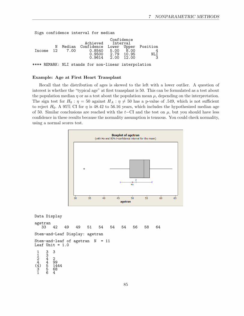
Example: Age at First Heart Transplant

Recall that the distribution of ages is skewed to the left with a lower outlier. A question ofinterest is whether the “typical age” at first transplant is 50. This can be formulated as a test aboutthe population median η or as a test about the population mean µ, depending on the interpretation.The sign test for H0 : η = 50 against HA : η 6= 50 has a p-value of .549, which is not sufficientto reject H0. A 95% CI for η is 48.42 to 56.16 years, which includes the hypothesized median ageof 50. Similar conclusions are reached with the t−CI and the test on µ, but you should have lessconfidence in these results because the normality assumption is tenuous. You could check normality,using a normal scores test.

Data Display

agetran33 42 49 49 51 54 54 54 56 58 64

Stem-and-Leaf Display: agetran

Stem-and-leaf of agetran N = 11Leaf Unit = 1.0

1 3 31 32 4 24 4 99(4) 5 14443 5 681 6 4

85


Descriptive Statistics: agetran

Variable N N* Mean SE Mean StDev Minimum Q1 Median Q3 Maximumagetran 11 0 51.27 2.49 8.26 33.00 49.00 54.00 56.00 64.00

One-Sample T: agetran

Test of mu = 50 vs not = 50

Variable N Mean StDev SE Mean 95% CI T Pagetran 11 51.2727 8.2594 2.4903 (45.7240, 56.8215) 0.51 0.620

Sign Test for Median: agetran

Sign test of median = 50.00 versus not = 50.00

N Below Equal Above P Medianagetran 11 4 0 7 0.5488 54.00

Sign CI: agetran



N Median Confidence Lower Upper Positionagetran 11 54.00 0.9346 49.00 56.00 3

0.9500 48.42 56.16 NLI0.9883 42.00 58.00 2

Wilcoxon Signed Rank Procedures

The Wilcoxon procedure assumes you have a random sample from a population with a symmetricfrequency curve. The curve need not be normal. The test and CI can be viewed as procedures foreither the population median or mean.

To illustrate the computation of the Wilcoxon statistic W , suppose you wish to test H0 : µ =µ0 = 10 on the data below. The test statistic requires us to compute the signs of Xi − µ0 andthe ranks of |Xi − µ0|. Ties in |Xi − µ0| get the average rank and observations at µ0 (here 10)are always discarded. The Wilcoxon statistic is the sum of the signed ranks for observationsabove µ0 = 10. For us

W = 6 + 4.5 + 8 + 2 + 4.5 + 7 = 32.

Xi Xi − 10 sign |Xi − 10| rank sign*rank20 10 + 10 6 618 8 + 8 4.5 4.523 13 + 13 8 85 -5 - 5 3 -314 4 + 4 2 28 -2 - 2 1 -118 8 + 8 4.5 4.522 12 + 12 7 7

86


The sum of all ranks is always .5m(m + 1), where m is the sample size. If H0 is true, youexpect W to be approximately .5 ∗ .5m(m + 1) = .25m(m + 1). Why? Recall that W adds up theranks for observations above µ0. If H0 is true, you expect 1/2 of all observations to be above µ0,assuming the population distribution is symmetric. The ranks of observations above µ0 should addto approximately 1/2 times the sum of all ranks. You reject H0 in favor of HA : µ 6= µ0 if W ismuch larger than, or much smaller than .25m(m+1). One sided tests can also be constructed. TheWilcoxon CI for µ is computed in a manner analogous to that described for the sign CI.

Here, m = 8 so the sum of all ranks is .5 ∗ 8 ∗ 9 = 36 (check yourself). The expected value ofW is .5 ∗ .5 ∗ 8 ∗ 9 = 18. Is the observed value of W far from the expected value? To formallyanswer this question, we need to use the Wilcoxon procedures, which are implemented in Minitabby following the sequence: Stat > Nonparametrics > 1-Sample Wilcoxon.

Example: Play Data

The boxplot indicates that the distribution is fairly symmetric, so the Wilcoxon method isreasonable (so is a t-CI and test). The p-value for testing H0 : µ = 10 against a two-sidedalternative is .059. This would not lead to rejecting H0 at the 5% level.

Although I asked for a 95% CI, I got a 94.1% CI. The W test statistic is discrete, so not allconfidence levels are achievable. Minitab gives the closest possible level. I underlined the estimatedmedian of 16.5 given by the CI procedure. This disagrees with the median you get in the datadescription. The CI median is computed using Walsh averages - see the Minitab help for anexplanation.

Data Display

data20 18 23 5 14 8 18 22

Descriptive Statistics: Income

Variable N N* Mean SE Mean StDev Minimum Q1 Median Q3 MaximumIncome 12 0 100.9 91.8 318.0 0.0 2.8 7.0 11.0 1110.0

One-Sample T: data


Variable N Mean StDev SE Mean 95% CI T Pdata 8 16.0000 6.5247 2.3068 (10.5452, 21.4548) 2.60 0.035

Wilcoxon Signed Rank Test: data

Test of median = 10.00 versus median not = 10.00

Nfor Wilcoxon Estimated

N Test Statistic P Mediandata 8 8 32.0 0.059 16.50

Wilcoxon Signed Rank CI: data

ConfidenceEstimated Achieved Interval

N Median Confidence Lower Upperdata 8 16.5 94.1 11.0 21.0

----

87


Nonparametric Analyses of Paired Data

Nonparametric methods for single samples can be used to analyze paired data because the differencebetween responses within pairs is the unit of analysis.

Example: Sleep Remedies

I will illustrate Wilcoxon methods on the paired comparison of two remedies A and B forinsomnia. The number of hours of sleep gained on each method was recorded. Unlike the parametricpaired t−test, you must create the sample of differences to do the non-parametric analysis inMinitab.

The boxplot shows that distribution of differences is reasonably symmetric but not normal.Recall that the Shapiro-Wilk test of normality was significant at the 5% level (p-value=.035). Itis sensible to use the Wilcoxon procedure on the differences. Let µB be the population mean sleepgain on remedy B, and µA be the population mean sleep gain on remedy A. You are 94.7% confidentthat µB −µA is between 0.8 and 2.7 hours. Putting this another way, you are 94.7% confident thatµB exceeds µA by between 0.8 and 2.7 hours. The p-value for testing H0 : µB − µA = 0 againsta two-sided alternative is .008, which strongly suggests that µB 6= µA. This agrees with the CI.Note that the t-CI and test give qualitatively similar conclusions as the Wilcoxon methods, but thet−test p-value is about twice as large.

If you are uncomfortable with the symmetry assumption, you could use the sign CI for thepopulation median difference between B and A. I will note that a 95% CI for the median differencegoes from 0.93 to 2.01 hours.

Data Display

diffRow a b (b-a)

1 0.7 1.9 1.22 -1.6 0.8 2.43 -0.2 1.1 1.34 -1.2 0.1 1.3

88


5 0.1 -0.1 -0.26 3.4 4.4 1.07 3.7 5.5 1.88 0.8 1.6 0.89 0.0 4.6 4.6

10 2.0 3.0 1.0

One-Sample T: diff (b-a)


Variable N Mean StDev SE Mean 95% CI T Pdiff (b-a) 10 1.52000 1.27174 0.40216 (0.61025, 2.42975) 3.78 0.004

Wilcoxon Signed Rank CI: diff (b-a)

ConfidenceEstimated Achieved Interval

N Median Confidence Lower Upperdiff (b-a) 10 1.30 94.7 0.80 2.70

Wilcoxon Signed Rank Test: diff (b-a)

Test of median = 0.000000 versus median not = 0.000000

Nfor Wilcoxon Estimated

N Test Statistic P Mediandiff (b-a) 10 10 54.0 0.008 1.300

Sign CI: diff (b-a)



N Median Confidence Lower Upper Positiondiff (b-a) 10 1.250 0.8906 1.000 1.800 3

0.9500 0.932 2.005 NLI0.9785 0.800 2.400 2

89


Comments on One-Sample Nonparametric Methods

For this discussion, I will assume that the underlying population distribution is (approximately)symmetric, which implies that population means and medians are equal (approximately). Forsymmetric distributions the t, sign, and Wilcoxon procedures are all appropriate.

If the underlying population distribution is extremely skewed, you can use the sign procedureto get a CI for the population median. Alternatively, as illustrated on HW 2, you can transformthe data to a scale where the underlying distribution is nearly normal, and then use the classicalt−methods. Moderate degrees of skewness will not likely have a big impact on the standard t−testand CI.

The one-sample t−test and CI are optimal when the underlying population frequency curve isnormal. Essentially this means that the t−CI is, on average, narrowest among all CI procedureswith given level, or that the t-test has the highest power among all tests with a given size. Thewidth of a CI provides a measure of the sensitivity of the estimation method. For a given level CI,the narrower CI better pinpoints the unknown population mean.

With heavy-tailed symmetric distributions, the t-test and CI tend to be conservative. Thus,for example, a nominal 95% t−CI has actual coverage rates higher than 95%, and the nominal5% t-test has an actual size smaller than 5%. The t−test and CI possess a property that iscommonly called robustness of validity. However, data from heavy-tailed distributions canhave a profound effect on the sensitivity of the t-test and CI. Outliers can dramatically inflate thestandard error of the mean, causing the CI to be needlessly wide, and tests to have diminished power(outliers typically inflate p-values for the t−test). The sign and Wilcoxon procedures downweightthe influence of outliers by looking at sign or signed-ranks instead of the actual data values. Thesetwo nonparametric methods are somewhat less efficient than the t-methods when the population isnormal (efficiency is about .64 and .96 for the sign and Wilcoxon methods relative to the normalt-methods, where efficiency is the ratio of sample sizes needed for equal power), but can be infinitelymore efficient with heavier than normal tailed distributions. In essence, the t-methods do not havea robustness of sensitivity.

Nonparametric methods have gained widespread acceptance in many scientific disciplines, butnot all. Scientists in some disciplines continue to use classical t−methods because they believethat the methods are robust to non-normality. As noted above, this is a robustness of validity, notsensitivity. This misconception is unfortunate, and results in the routine use of methods that areless powerful than the non-parametric techniques. Scientists need to be flexible and adapttheir tools to the problem at hand, rather than use the same tool indiscriminately! Ihave run into suspicion that use of nonparametric methods was an attempt to “cheat” in some way– properly applied, they are excellent tools that should be used.

A minor weakness of nonparametric methods is that they do not easily generalize to complexmodelling problems. A great deal of progress has been made in this area, but most software packageshave not included the more advanced techniques.

Nonparametric statistics used to refer almost exclusively to the set of methods such as we havebeen discussing that provided analogs like tests and CIs to the normal theory methods withoutrequiring the assumption of sampling from normal distributions. There is now a large area ofstatistics also called nonparametric methods not focused on these goals at all. In our departmentwe have a course titled “Nonparametric Curve Estimation & Image Reconstruction”, where the

90


focus is much more general than relaxing an assumption of normality. In that sense, what we arecovering in this course could be considered “classical” nonparametrics.

(Wilcoxon-) Mann-Whitney Two Sample Procedure

The WMW procedure assumes you have independent random samples from the two populations,and assumes that the populations have the same shapes and spreads (the frequency curves for thetwo populations are ”shifted” versions of each other - see below). The frequency curves are notrequired to be symmetric. The WMW procedures give a CI and tests on the difference η1 − η2

between the two population medians. If the populations are symmetric, then the methods applyto µ1 − µ2.

-5 0 5 10 15 20

0.0

0.05

0.10

0.15

0.20

0 5 10 15

0.0

0.05

0.10

0.15

The Minitab on-line help explains the exact WMW procedure actually calculated. I will discussa very good approximation to the exact method that is easier to understand. The WMW procedureis based on ranks. The two samples are combined, ranked from smallest to largest (1=smallest) andseparated back into the original samples. If the two populations have equal medians, you expectthe average rank in the two samples to be roughly equal. The WMW test computes a classical twosample t-test using the pooled variance on the ranks to assess whether the sample mean ranks aresignificantly different.

The WMW test and CI are implemented in Minitab by following these steps:Stat > Nonparametrics > Mann-Whitney. The data must be UNSTACKED. The test and CI aregenerated simultaneously. A two-sided CI is given, even if a one-sided test is requested.

Example: Comparison of Cooling Rates of Walker and Uwet Meteorites.

The Uwet and Walker Co. data were read into two columns of the Minitab worksheet. Aprimary interest is comparing the population “typical” cooling rate measurements.

91


Data Display

Row Uwet Walker cool meteorite ranks1 0.21 0.69 0.21 Uwet 9.02 0.25 0.23 0.25 Uwet 13.03 0.16 0.10 0.16 Uwet 7.54 0.23 0.03 0.23 Uwet 11.55 0.47 0.56 0.47 Uwet 15.06 1.20 0.10 1.20 Uwet 19.07 0.29 0.01 0.29 Uwet 14.08 1.10 0.02 1.10 Uwet 18.09 0.16 0.04 0.16 Uwet 7.5

10 0.22 0.69 Walker 17.011 0.23 Walker 11.512 0.10 Walker 5.513 0.03 Walker 3.014 0.56 Walker 16.015 0.10 Walker 5.516 0.01 Walker 1.017 0.02 Walker 2.018 0.04 Walker 4.019 0.22 Walker 10.0

Descriptive Statistics: cool

Variable meteorite N N* Mean SE Mean StDev Minimum Q1 Mediancool Uwet 9 0 0.452 0.136 0.407 0.160 0.185 0.250

Walker 10 0 0.2000 0.0756 0.2390 0.0100 0.0275 0.1000

Variable meteorite Q3 Maximumcool Uwet 0.785 1.200

Walker 0.3125 0.6900

The boxplots, stem and leaf, and normal scores plots show that the distributions are ratherskewed to the right. Both the AD and RJ tests of normality indicate that a normality assumptionis unreasonable for each population.

I carried out the standard two-sample procedures to see what happens. The pooled variance andSatterthwaithe results are comparable, which is expected because the sample standard deviationsand sample sizes are roughly equal. Both tests indicate that the mean cooling rates for Uwet andWalker Co. meteorites are not significantly different at the 10% level. You are 95% confident thatthe mean cooling rate for Uwet is at most .1 less, and no more than .6 greater than that for Walker.(in degrees per million years).

Two-Sample T-Test and CI: cool, meteorite

92


Two-sample T for cool

meteorite N Mean StDev SE MeanUwet 9 0.452 0.407 0.14Walker 10 0.200 0.239 0.076

Difference = mu (Uwet) - mu (Walker)Estimate for difference: 0.25222295% CI for difference: (-0.066627, 0.571071)T-Test of difference = 0 (vs not =): T-Value = 1.67 P-Value = 0.113 DF = 17Both use Pooled StDev = 0.3289

Two-Sample T-Test and CI: cool, meteorite

Two-sample T for cool


Difference = mu (Uwet) - mu (Walker)Estimate for difference: 0.25222295% CI for difference: (-0.086133, 0.590578)T-Test of difference = 0 (vs not =): T-Value = 1.62 P-Value = 0.130 DF = 12

Given the marked skewness, a nonparametric procedure is more appropriate. The Wilcoxon-Mann-Whitney comparison of population medians is reasonable. Why? The WMW test of equalpopulation medians is significant (barely) at the 5% level. You are 95% confident that mediancooling rate for Uwet exceeds that for Walker by between 0+ and .45 degrees per million years.

The difference between the WMW and t-test p-values and CI lengths (i.e. the WMW CI isnarrower and the p-value smaller) reflects the effect of the outliers on the sensitivity of the standardtests and CI.

In the worksheet, I computed the ranks by first stacking the data, then following Data > Rank.I conducted a two-sample t-test on ranks to show you that the p-value is close to the WMW p-value,as expected.

Descriptive Statistics: ranks <- describe ranks, to think about WMW results

Variable meteorite N N* Mean SE Mean StDev Minimum Q1 Medianranks Uwet 9 0 12.72 1.41 4.24 7.50 8.25 13.00

Walker 10 0 7.55 1.82 5.75 1.00 2.75 5.50

Variable meteorite Q3 Maximumranks Uwet 16.50 19.00

Walker 12.63 17.00

Two-Sample T-Test and CI: ranks, meteorite

Two-sample T for ranks


Difference = mu (Uwet) - mu (Walker)

93


Estimate for difference: 5.1722295% CI for difference: (0.23049, 10.11395) <<<<<---- NOT InterpretableT-Test of difference = 0 (vs not =): T-Value = 2.21 P-Value = 0.041 DF = 17Both use Pooled StDev = 5.0978

Mann-Whitney Test and CI: Uwet, Walker

N MedianUwet 9 0.2500Walker 10 0.1000

Point estimate for ETA1-ETA2 is 0.175095.5 Percent CI for ETA1-ETA2 is (-0.0002,0.4501) <<<<<--- Can’t get exact 95% CIW = 114.5Test of ETA1 = ETA2 vs ETA1 not = ETA2 is significant at 0.0500The test is significant at 0.0497 (adjusted for ties)

Example: Newcombe’s Data

Experiments of historical importance were performed beginning in the eighteenth century todetermine such physical constants as the mean density of the earth, the distance from the earth tothe sun, and the velocity of light. An interesting series of experiments to determine the velocityof light was begun in 1875. The first method used, and reused with refinements several timesthereafter, was the rotating mirror method. In this method a beam of light is reflected off arapidly rotating mirror to a fixed mirror at a carefully measured distance from the source. Thereturning light is re-reflected from the rotating mirror at a different angle, because the mirror hasturned slightly during the passage of the corresponding light pulses. From the speed of rotationof the mirror and from careful measurements of the angular difference between the outward-boundand returning light beams, the passage time of light can be calculated for the given distance.After averaging several calculations and applying various corrections, the experimenter can combinemean passage time and distance for a determination of the velocity of light. Simon Newcombe, adistinguished American scientist, used this method during the year 1882 to generate the passagetime measurements given below, in microseconds. The travel path for this experiment was 3721meters in length, extending from Ft. Meyer, on the west bank of the Potomac River in Washington,D.C. to a fixed mirror at the base of the Washington Monument.

The problem is to determine a 95% CI for the “true” passage time, which is taken to be themean of the population of measurements that were or could have been taken by this experiment.

Data Display

Passage24.828 24.827 24.824 24.831 24.836 24.837 24.836 24.82724.826 24.839 24.829 24.826 24.816 24.821 24.819 24.82824.825 24.826 24.827 24.833 24.828 24.827 24.833 24.84024.825 24.824 24.825 24.828 24.830 24.828 24.826 24.82424.828 24.824 24.798 24.830 24.820 24.821 24.826 24.82224.827 24.832 24.825 24.829 24.834 24.829 24.823 24.83624.828 24.830 24.836 24.831 24.832 24.832 24.816 24.75624.822 24.829 24.832 24.829 24.832 24.823 24.827 24.82424.825 24.823

94


The data set is skewed to the left, due to the presence of two extreme outliers that couldpotentially be misrecorded observations. Without additional information I would be hesitant toapply normal theory methods (the t-test), even though the sample size is “large”. Basically, folkloresays you can apply standard normal theory methods in large samples. This is true, but how largethe sample must be depends on how skewed, or heavy tailed, the underlying population distributionis. Furthermore, the t-test still suffers from a lack of robustness of sensitivity, even in large samples.A formal normal scores test (not provided) would reject, at the 0.01 level, the normality assumptionneeded for the standard methods.

The table below gives 95% t, sign and Wilcoxon CIs. I am more comfortable with the signCI for the population median than the Wilcoxon method, which assumes symmetry. The questionasks for CI for a population mean, but this is probably because the book I got this problem fromwas illustrating methods for means!

Method Limitst 24.8236 - 24.8289

sign 24.8260 - 24.8284Wilcoxon 24.8260 - 24.8285

Note the big difference between the nonparametric and the t-CI. The nonparametric CIs are about1/2 as wide as the t-CI. This reflects the impact that outliers have on the standard deviation, whichdirectly influences the CI width.

Computation note: Minitab is pretty poor at formatting output for data like this with thenonparametric procedures. When it printed the lower and upper bounds for the sign and WilcoxonCIs, it reported both upper and lower bounds of 24.83 – a fairly useless report. The problem isthe number of digits recorded in the original data. To get the values above I subtracted 24.7 fromthe original values, calculated CIs, and added 24.7 back to the CI limits. SAS tends to print aridiculous number of digits; Minitab usually makes prettier output, but they should be more carefulhere.

95


Alternative Analyses for ANOVA and Planned Comparisons

The classical ANOVA assumes that the populations have normal frequency curves and the popu-lations have equal variances (or spreads). You learned formal tests for these assumptions earlier.When the assumptions do not hold, you can try one of the following two approaches. Before de-scribing alternative methods, I will note that deviations from normality in one or more samplesmight be expected in a comparison involving many samples. You should downplay small deviationsfrom normality in problems involving many samples.

Kruskal-Wallis ANOVA

The Kruskal-Wallis (KW) test is a non-parametric method for testing the hypothesis of equalpopulation medians against the alternative that not all population medians are equal. The pro-cedure assumes you have independent random samples from populations with frequency curveshaving identical shapes and spreads.

The KW ANOVA is essentially the standard ANOVA based on ranked data. That is, wecombine the samples, rank the observations from smallest to largest, and then return the ranks tothe original samples and do the standard ANOVA using the ranks.

The KW ANOVA is a multiple sample analog of the Wilcoxon-Mann-Whitney two sampleprocedure. Hence, multiple comparisons for a KW analysis, be they FSD or Bonferroni comparisons,are based on the two sample WMW procedure.

Transforming Data

The distributions in many data sets are skewed to the right with outliers. If the sample spreads, says and IQR, increase with an increasing mean or median, you can often transform data to a scalewhere the normality and the constant spread assumption are more nearly satisfied. The transformeddata are analyzed using the standard ANOVA. The two most commonly used transforms for thisproblem are the square root and natural logarithm, provided the data are non-negative. I will giveyou some idea why this might work in class.

If the original distributions are nearly symmetric, but heavy tailed, non-linear transformationswill tend to destroy the symmetry. Many statisticians recommend methods based on trimmedmeans for such data. These methods are not commonly used by other researchers.

Example: Hydrocarbon (HC) Emissions Data

These data are the HC emissions at idling speed, in ppm, for automobiles of different years ofmanufacture. The data are a random sample of all automobiles tested at an Albuquerque shoppingcenter. (It looks like we need to find some newer cars!)

The standard ANOVA shows significant differences among the mean HC emissions. However,the standard ANOVA is inappropriate because the distributions are extremely skewed to the rightdue to presence of outliers in each sample.

Data Display

96


Row Pre-63 63-7 68-9 70-1 72-41 2351 620 1088 141 1402 1293 940 388 359 1603 541 350 111 247 204 1058 700 558 940 205 411 1150 294 882 2236 570 2000 211 494 607 800 823 460 306 208 630 1058 470 200 959 905 423 353 100 360

10 347 900 71 300 7011 405 241 223 22012 780 2999 190 40013 270 199 140 21714 188 880 5815 353 200 23516 117 223 188017 188 20018 435 17519 940 8520 241

Descriptive Statistics: Pre-63, 63-7, 68-9, 70-1, 72-4

Variable N N* Mean SE Mean StDev Minimum Q1 Median Q3 MaximumPre-63 10 0 891 187 592 347 509 715 1117 235163-7 13 0 801 126 455 270 414 780 999 200068-9 16 0 506 177 708 71 191 324 468 299970-1 20 0 381.5 64.4 287.9 100.0 192.5 244.0 479.3 940.072-4 19 0 244.1 94.2 410.8 20.0 60.0 160.0 223.0 1880.0

One-way ANOVA: Pre-63, 63-7, 68-9, 70-1, 72-4

Source DF SS MS F PFactor 4 4226834 1056709 4.34 0.003Error 73 17759968 243287Total 77 21986802

S = 493.2 R-Sq = 19.22% R-Sq(adj) = 14.80%

97


Individual 95% CIs For Mean Based onPooled StDev

Level N Mean StDev ---------+---------+---------+---------+Pre-63 10 890.6 591.6 (----------*---------)63-7 13 801.5 454.9 (--------*--------)68-9 16 506.3 707.8 (-------*-------)70-1 20 381.5 287.9 (-------*------)72-4 19 244.1 410.8 (------*-------)

---------+---------+---------+---------+300 600 900 1200

Pooled StDev = 493.2

The boxplots show that the typical HC emissions appear to increase as the age of car increases(the simplest description). Although the spread in the samples, as measured by the IQR, alsoincreases as age increases, I am more comfortable with the KW ANOVA, in part because the KWanalysis is not too sensitive to differences in spreads among samples. This point is elaborated uponlater. As described earlier, the KW ANOVA is essentially an ANOVA based on the ranks. I givebelow the ANOVA based on ranks and the output from the KW procedure. They give similar p-values, and lead to the conclusion that there are significant differences among the population medianHC emissions. A simple description is that the population median emission tends to increase withthe age of the car. You should follow up this analysis with Mann-Whitney multiple comparisons.

The KW ANOVA is conducted in Minitab by following these steps: Stat > Nonparametrics> Kruskal-Wallis. The data must be STACKED, and you need to specify the response variable,and the factor that defines the groups.

One-way ANOVA: hce_rank versus Year

Source DF SS MS F PYear 4 16329 4082 12.85 0.000Error 73 23200 318Total 77 39529

Kruskal-Wallis Test: HCE versus Year

Kruskal-Wallis Test on HCE

Year N Median Ave Rank Z63-7 13 780.0 58.6 3.3368-9 16 323.5 37.4 -0.4170-1 20 244.0 36.6 -0.6772-4 19 160.0 20.3 -4.25Pre-63 10 715.0 60.4 3.12Overall 78 39.5

H = 31.80 DF = 4 P = 0.000H = 31.81 DF = 4 P = 0.000 (adjusted for ties)

It is common to transform the data to a log scale when the spread increases as the median ormean increases. The data have already been STACKED, so it is straightforward to transform the

98


HCE levels to the log scale using the Minitab calculator. Side-by-side boxplots of the transformeddata are given on the same page as the boxplots of the untransformed data.

After transformation, the samples have roughly the same spread (IQR and s) and shape. Thetransformation does not completely eliminate the outliers. However, I am more comfortable with astandard ANOVA on this scale than with the original data. A difficulty here is that the ANOVA iscomparing population mean log HC emission. Summaries for the ANOVA on the log hydrocarbonemissions levels are given below.

One-way ANOVA: hce_rank versus Year

Source DF SS MS F PYear 4 16329 4082 12.85 0.000Error 73 23200 318Total 77 39529

S = 17.83 R-Sq = 41.31% R-Sq(adj) = 38.09%

Individual 95% CIs For Mean Based onPooled StDev

Level N Mean StDev --+---------+---------+---------+-------63-7 13 58.58 12.67 (------*------)68-9 16 37.44 21.16 (-----*-----)70-1 20 36.58 18.82 (----*-----)72-4 19 20.29 19.08 (-----*----)Pre-63 10 60.35 11.89 (------*-------)

--+---------+---------+---------+-------15 30 45 60

Pooled StDev = 17.83

The boxplot of the log-transformed data reinforces the reasonableness of the original KW anal-ysis. Why? The log-transformed distributions have fairly similar shapes and spreads, so a KWanalysis on these data is sensible. The ranks for the original and log-transformed data are identi-cal, so the KW analyses on the log-transformed data and the original data must lead to the sameconclusions. This suggests that the KW ANOVA is not overly sensitive to differences in spreadsamong the samples.

99


There are two reasonable analyses here: the standard ANOVA using log HC emissions, and theKW analysis of the original data. The first analysis gives a comparison of mean log-HC emissions.The second involves a comparison of median HC emissions. A statistician would present bothanalyses to the scientist who collected the data to make a decision on which was more meaningful(independently of the results!). Multiple comparisons would be performed relative to the selectedanalysis.

Example: Hodgkin’s Disease Study

Plasma bradykininogen levels were measured in normal subjects, in patients with active Hodgkin’sdisease, and in patients with inactive Hodgkin’s disease. The globulin bradykininogen is the pre-cursor substance for bradykinin, which is thought to be a chemical mediator of inflammation. Thedata (in micrograms of bradykininogen per milliliter of plasma) are displayed below. The threesamples are denoted by nc for normal controls, ahd for active Hodgkin’s disease patients, and ihdfor inactive Hodgkin’s disease patients.

The medical investigators wanted to know if the three samples differed in their bradykininogenlevels. Carry out the statistical analysis you consider to be most appropriate, and state yourconclusions to this question.

Data Display

Data Display

Row nc ahd ihd1 5.37 3.96 5.372 5.80 3.04 10.603 4.70 5.28 5.024 5.70 3.40 14.305 3.40 4.10 9.906 8.60 3.61 4.277 7.48 6.16 5.758 5.77 3.22 5.039 7.15 7.48 5.7410 6.49 3.87 7.8511 4.09 4.27 6.8212 5.94 4.05 7.9013 6.38 2.40 8.3614 9.24 5.81 5.7215 5.66 4.29 6.0016 4.53 2.77 4.7517 6.51 4.40 5.8318 7.00 7.3019 6.20 7.5220 7.04 5.3221 4.82 6.0522 6.73 5.6823 5.26 7.5724 5.6825 8.9126 5.3927 4.4028 7.13

Descriptive Statistics: nc, ahd, ihd

Variable N N* Mean SE Mean StDev Minimum Q1 Median Q3 Maximumnc 23 0 6.081 0.284 1.362 3.400 5.260 5.940 7.000 9.240ahd 17 0 4.242 0.316 1.303 2.400 3.310 4.050 4.840 7.480ihd 28 0 6.791 0.411 2.176 4.270 5.375 5.915 7.780 14.300

100


Although the spread (IQR, s) in the ihd sample is somewhat greater than the spread in the othersamples, the presence of skewness and outliers in the boxplots is a greater concern regarding theuse of the classical ANOVA. The shapes and spreads in the three samples are roughly identical, soa Kruskal-Wallis nonparametric ANOVA appears ideal. As a sidelight, I transformed plasma levelsto a log scale to reduce the skewness and eliminate the outliers. The boxplots of the transformeddata show reasonable symmetry across groups, but outliers are still present. I will stick with theKruskal-Wallis ANOVA (although it would not be much of a problem to use the classical ANOVAon transformed data).

Let ηnc = population median plasma level for normal controls, ηahd = population medianplasma level for active Hodgkin’s disease patients, and ηihd = population median plasma level forinactive Hodgkin’s disease patients. The KW test of H0 : ηnc = ηahd = ηihd is highly significant(p−value = .000), suggesting differences among the population median plasma levels. The Kruskal-Wallis ANOVA summary is given below.

Kruskal-Wallis Test: b_level versus Group

Kruskal-Wallis Test on b_level

Group N Median Ave Rank Znc 23 5.940 38.3 1.14ahd 17 4.050 15.9 -4.47ihd 28 5.915 42.6 2.83Overall 68 34.5

H = 20.56 DF = 2 P = 0.000H = 20.57 DF = 2 P = 0.000 (adjusted for ties)

I followed up the KW ANOVA with Bonferroni comparisons of the samples, using the Mann-Whitney two sample procedure. There are three comparisons, so an overall FER of .05 is achievedby doing the individual tests at the .05/3=.0167 level. Alternatively, you can use 98.33% CI fordifferences in population medians.

Remember that the WMW two-sample comparisons requires UNSTACKED data, whereas theKW required STACKED data!

101


Mann-Whitney Test and CI: nc, ahd

N Mediannc 23 5.940ahd 17 4.050

Point estimate for ETA1-ETA2 is 1.91098.4 Percent CI for ETA1-ETA2 is (0.860,2.900)W = 605.0Test of ETA1 = ETA2 vs ETA1 not = ETA2 is significant at 0.0003The test is significant at 0.0003 (adjusted for ties)

Mann-Whitney Test and CI: nc, ihd

N Mediannc 23 5.940ihd 28 5.915

Point estimate for ETA1-ETA2 is -0.34598.3 Percent CI for ETA1-ETA2 is (-1.559,0.680)W = 552.5Test of ETA1 = ETA2 vs ETA1 not = ETA2 is significant at 0.3943The test is significant at 0.3943 (adjusted for ties)

Mann-Whitney Test and CI: ahd, ihd

N Medianahd 17 4.050ihd 28 5.915

Point estimate for ETA1-ETA2 is -2.14598.4 Percent CI for ETA1-ETA2 is (-3.500,-1.320)W = 209.0Test of ETA1 = ETA2 vs ETA1 not = ETA2 is significant at 0.0000The test is significant at 0.0000 (adjusted for ties)

The only comparison with a p-value greater than .0167 involved the nc and ihd samples. Thecomparison leads to two groups, and is consistent with what we see in the boxplots.

ahd nc ihd--- --------

You have sufficient evidence to conclude that the plasma bradykininogen levels for active Hodgkin’sdisease patients is lower than the population median levels for normal controls, and for patients withinactive Hodgkin’s disease. You do not have sufficient evidence to conclude that the populationmedian levels for normal controls and for patients with inactive Hodgkin’s disease are different.The CIs give an indication of size of differences in the population medians.

102


Planned Comparisons

Bonferroni multiple comparisons are generally preferred to Fisher’s least significant difference ap-proach. Fisher’s method does not control the family error rate and produces too many spurioussignificant differences (claims of significant differences that are due solely to chance variation andnot to actual differences in population means). However, Bonferroni’s method is usually very con-servative when a large number of comparisons is performed - large differences in sample meansare needed to claim significance. A way to reduce this conservatism is to avoid doing all possiblecomparisons. Instead, one should, when possible, decide a priori (before looking at the data) whichcomparisons are of primary interest, and then perform only those comparisons.

For example, suppose a medical study compares five new treatments with a control (a six groupproblem). The medical investigator may not be interested in all 15 possible comparisons, but onlyin which of the five treatments differ on average from the control. Rather than performing the15 comparisons, each at the say .05/15 = .0033 level, she could examine the five comparisons ofinterest at the .05/5 = .01 level. By deciding beforehand which comparisons are of interest, she canjustify using a .01 level for the comparisons, instead of the more conservative .0033 level neededwhen doing all possible comparisons.

To illustrate this idea, consider the KW analysis of HC emissions. We saw that there aresignificant differences among the population median HC emissions. Given that the samples have anatural ordering

Sample Year of manufacture1 Pre 19632 63 - 673 68 - 694 70 - 715 72 - 74

you may primarily be interested in whether the population medians for cars manufactured inconsecutive samples are identical. That is, you may be primarily interested in the following 4comparisons:

Pre 1963 vs 63 - 6763 - 67 vs 68 - 6968 - 69 vs 70 - 7170 - 71 vs 72 - 74

A Bonferroni analysis would carry out each comparison at the .05/4 = .0125 level versus the .05/10= .005 level when all comparisons are done.

The following output was obtained from Minitab for doing these four comparisons, based onWilcoxon-Mann-Whitney two sample tests (why?). Two year-groups are claimed to be differentif the p-value is .0125 or below, or equivalently, if a 98.75% CI for the difference in populationmedians does not contain zero.

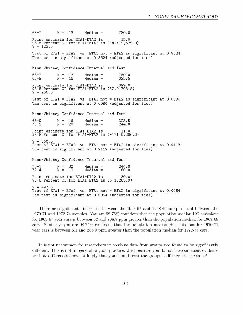
Mann-Whitney Confidence Interval and Test

Pre-63 N = 10 Median = 715.0

103


63-7 N = 13 Median = 780.0

Point estimate for ETA1-ETA2 is 15.098.8 Percent CI for ETA1-ETA2 is (-427.9,529.9)W = 123.5

Test of ETA1 = ETA2 vs ETA1 not = ETA2 is significant at 0.8524The test is significant at 0.8524 (adjusted for ties)


63-7 N = 13 Median = 780.068-9 N = 16 Median = 323.5

Point estimate for ETA1-ETA2 is 399.098.8 Percent CI for ETA1-ETA2 is (52.0,708.8)W = 256.0

Test of ETA1 = ETA2 vs ETA1 not = ETA2 is significant at 0.0080The test is significant at 0.0080 (adjusted for ties)


68-9 N = 16 Median = 323.570-1 N = 20 Median = 244.0

Point estimate for ETA1-ETA2 is 11.098.8 Percent CI for ETA1-ETA2 is (-171.0,206.0)

W = 300.0Test of ETA1 = ETA2 vs ETA1 not = ETA2 is significant at 0.9113The test is significant at 0.9112 (adjusted for ties)


70-1 N = 20 Median = 244.072-4 N = 19 Median = 160.0

Point estimate for ETA1-ETA2 is 130.098.8 Percent CI for ETA1-ETA2 is (6.1,285.9)

W = 497.5Test of ETA1 = ETA2 vs ETA1 not = ETA2 is significant at 0.0064The test is significant at 0.0064 (adjusted for ties)

There are significant differences between the 1963-67 and 1968-69 samples, and between the1970-71 and 1972-74 samples. You are 98.75% confident that the population median HC emissionsfor 1963-67 year cars is between 52 and 708.8 ppm greater than the population median for 1968-69cars. Similarly, you are 98.75% confident that the population median HC emissions for 1970-71year cars is between 6.1 and 285.9 ppm greater than the population median for 1972-74 cars.

It is not uncommon for researchers to combine data from groups not found to be significantlydifferent. This is not, in general, a good practice. Just because you do not have sufficient evidenceto show differences does not imply that you should treat the groups as if they are the same!

104


A Final ANOVA Comment

If the data distributions do not substantially deviate from normality, but the spreads are differentacross samples, you might consider the standard ANOVA followed with multiple comparisons usingtwo-sample tests based on Satterthwaite’s approximation.

105

7 nonparametric methods

Documents