7. Post Glacial Rebound

Ge 163 4/16/14-

Outline

• Overview • Order of magnitude estimate of mantle viscosity • Essentials of fluid mechanics • Viscosity • Stokes Flow • Biharmonic equation • Half-space model • Channel Flow • Deep Flow versus Channel Flow • Relaxation spectra • GPS constraint • GRACE Constraints • Latest models with variable viscosity

Fowler

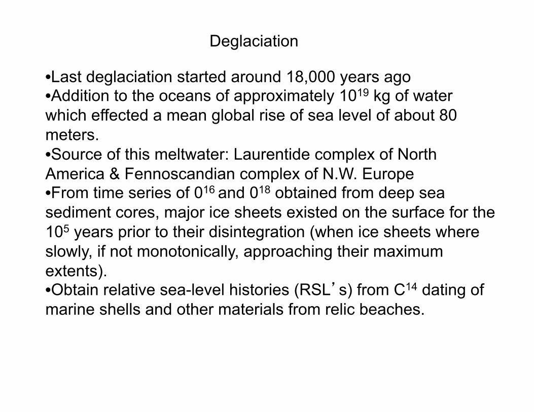
Deglaciation

• Last deglaciation started around 18,000 years ago • Addition to the oceans of approximately 1019 kg of water which effected a mean global rise of sea level of about 80 meters. • Source of this meltwater: Laurentide complex of North America & Fennoscandian complex of N.W. Europe • From time series of 016 and 018 obtained from deep sea sediment cores, major ice sheets existed on the surface for the 105 years prior to their disintegration (when ice sheets where slowly, if not monotonically, approaching their maximum extents). • Obtain relative sea-level histories (RSL’s) from C14 dating of marine shells and other materials from relic beaches.

Geophysical observations

• Correlation of ΔgFA with topography • Correlation of ΔgFA with geomorphologically inferred position of the ice sheets • Direct measurements of surface displacements with GPS • GRACE (time-dependent gravity)

Retreat of the Laurentide Ice Sheet

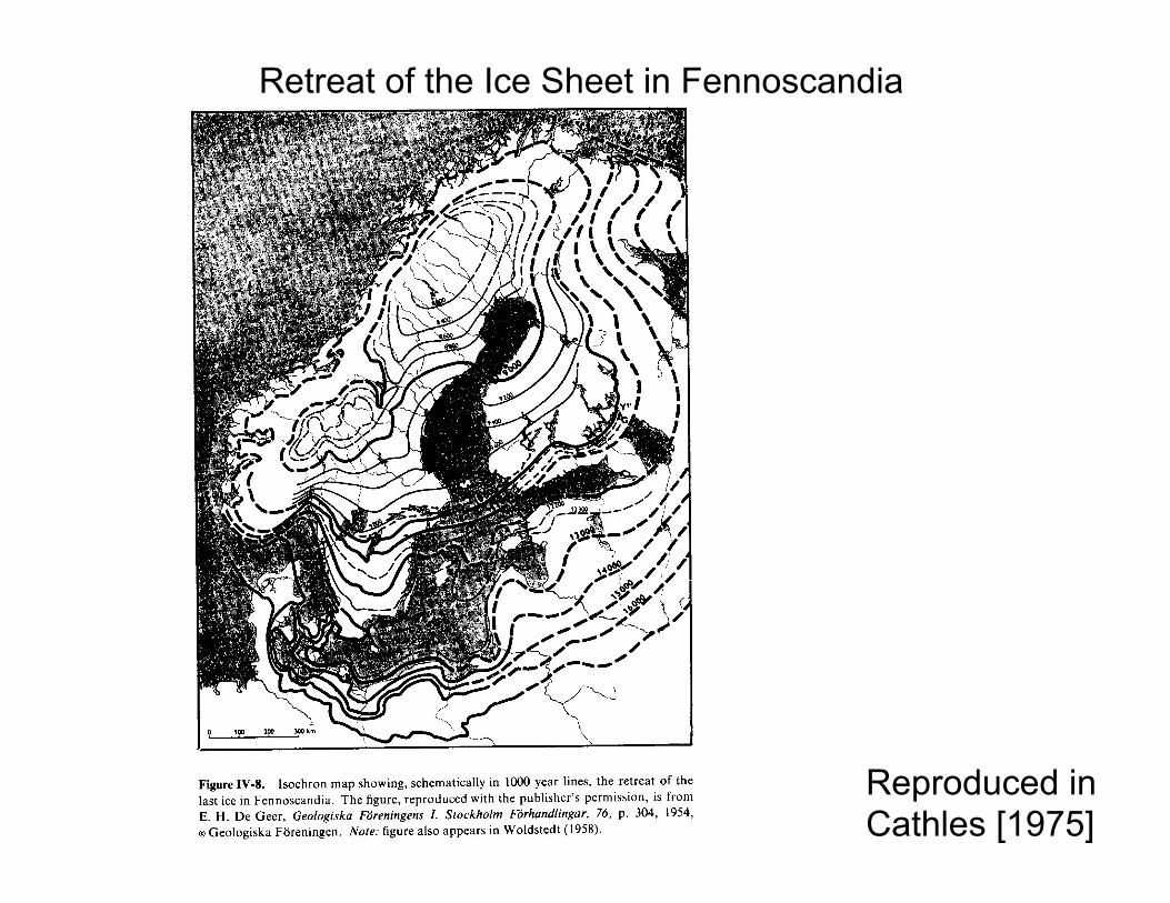
Reproduced in Cathles [1975]

Reproduced in Cathles [1975]

Retreat of the Ice Sheet in Fennoscandia

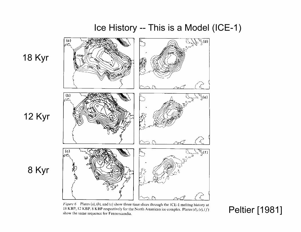
Ice History -- This is a Model (ICE-1)

Peltier [1981]

18 Kyr

12 Kyr

8 Kyr

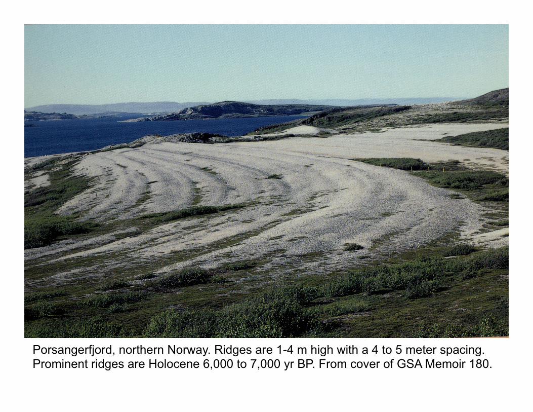
Porsangerfjord, northern Norway. Ridges are 1-4 m high with a 4 to 5 meter spacing. Prominent ridges are Holocene 6,000 to 7,000 yr BP. From cover of GSA Memoir 180.

Relative Sea Level (RSL) Curve

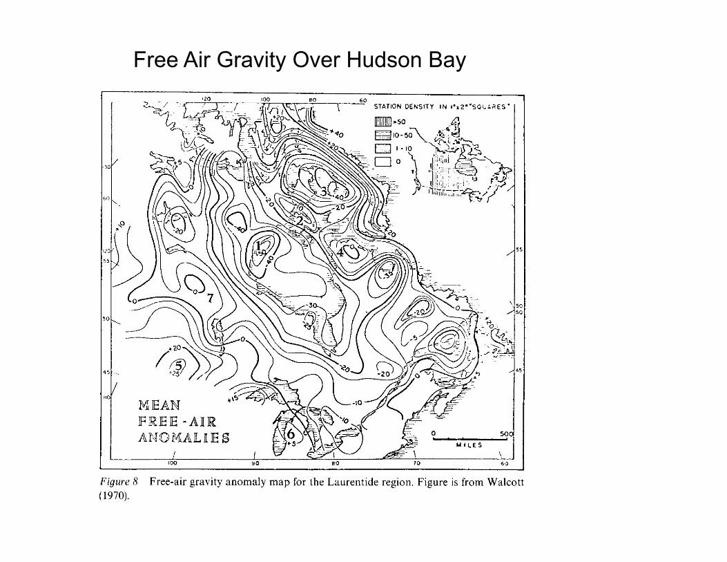
Free Air Gravity Over Hudson Bay

Gravity anomalies from 363 days of GRACE data (GGM02S)

From a Peltier paper

Using Oxygen Isotopes as a proxy for Ice volume

Order of Magnitude Estimate of Newtonian Viscosity of the mantle

L

h

h

σ = 2η εσ = ρgh

ε ≈hL

why?

⇒η =σ2 ε

~ ρghL2 h

η ~ ρghL2 h

Remaining uplift will be approximated with the Bouguer Formula

Δg = 2πρGh

h ≈ ΔgFA2πρG

⇒η ~ gΔgFAL4πG h

Laurentide Fennoscandia

Dimensions Length X width

4 x 106 2.5 x 106 m

2.25 x 106 1.35 x 106 m

Mean Free-air gravity anomaly

-35 mgal -16 mgal

Present rate of uplift

1.7 cm/yr 0.9 cm/yr

η [Dimensional scaling]

2 x 1022 Pa-s 1 x 1021 Pa-s

Using Rebound Parameters in Walcott[1973]

η ~ gΔgFAL

4πG h

Viscosity

We will need a ‘constitutive relation’, which for fluid mechanics relates strain rates to stress.

σ ij = − pδ ij + λ θδ ij + 2η εij

Bulk viscosity shear viscosity

dilitation

εij =12

∂ui∂x j

+∂uj

∂xi

⎛

⎝⎜⎞

⎠⎟ is the strain rate tensor; u is velocity

θ= εkk (dilitation)For an incompressible fluid (i.e. ∇ ⋅u = 0), εkk = 0⇒σ ij = − pδ ij + 2η εij

σ ij = − pδ ij + 2η εij We may think of η (the shear or 'dynamic viscosity') as a constant, but is it?

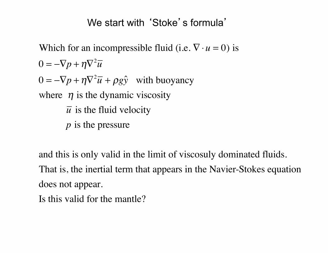
We start with ‘Stoke’s formula’

Which for an incompressible fluid (i.e. ∇ ⋅u = 0) is0 = −∇p +η∇2u0 = −∇p +η∇2u + ρgy with buoyancywhere η is the dynamic viscosity u is the fluid velocity p is the pressure

and this is only valid in the limit of viscosuly dominated fluids.That is, the inertial term that appears in the Navier-Stokes equationdoes not appear.Is this valid for the mantle?

NS: − ∇p +η∇2u + ρgy = ρ DuDt

Viscous forces are: η∇2u or η uL2

Inertial forces are proportional to

ρ DuDt ρ u ⋅∇( )u ρ u

2

LRatio of these forcesinertialviscous

~ ρu2

LL2

ηu=ρuLη

(ρ /η = υ, the kinematic viscosity)

=uLυ

≡ Re = Reynolds Number

A characteristic length scale

�

(η /ρ = ν, the kinematic viscosity)

Navier-Stokes

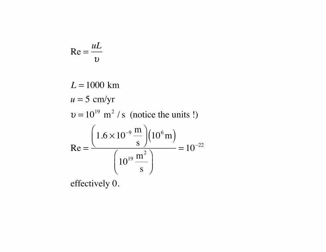
Re = uLυ

L = 1000 kmu = 5 cm/yrυ = 1019 m2 / s (notice the units !)

Re =1.6 ×10−9 m

s⎛⎝⎜

⎞⎠⎟ 106 m( )

1019 m2

s⎛⎝⎜

⎞⎠⎟

= 10−22

effectively 0.

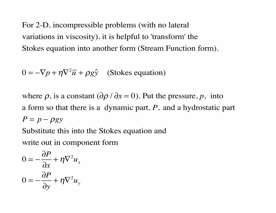
For 2-D, incompressible problems (with no lateral variations in viscosity), it is helpful to 'transform' theStokes equation into another form (Stream Function form).

0 = −∇p +η∇2u + ρgy (Stokes equation)

where ρ, is a constant (∂ρ / ∂x = 0). Put the pressure, p, into a form so that there is a dynamic part, P, and a hydrostatic partP = p − ρgySubstitute this into the Stokes equation and write out in component form

0 = −∂P∂x

+η∇2ux

0 = −∂P∂y

+η∇2uy

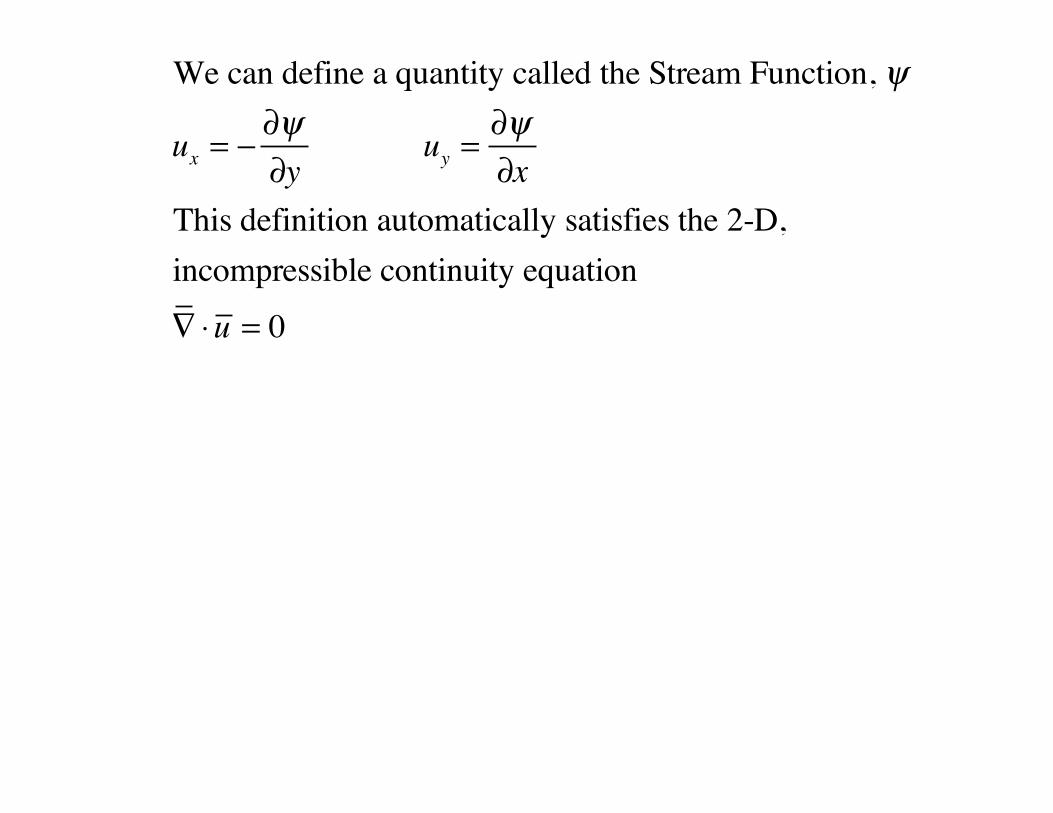
We can define a quantity called the Stream Function, ψ

ux = −∂ψ∂y

uy =∂ψ∂x

This definition automatically satisfies the 2-D,incompressible continuity equation

∇ ⋅u = 0

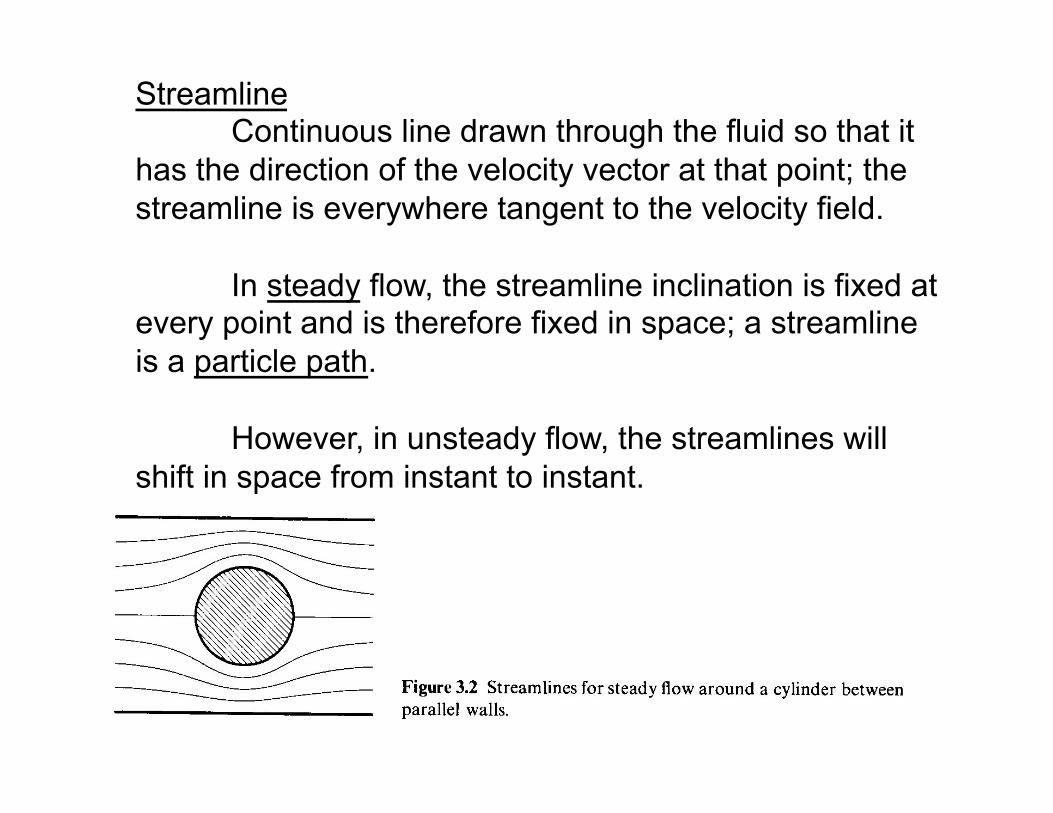
Streamline Continuous line drawn through the fluid so that it

has the direction of the velocity vector at that point; the streamline is everywhere tangent to the velocity field.

In steady flow, the streamline inclination is fixed at every point and is therefore fixed in space; a streamline is a particle path.

However, in unsteady flow, the streamlines will shift in space from instant to instant.

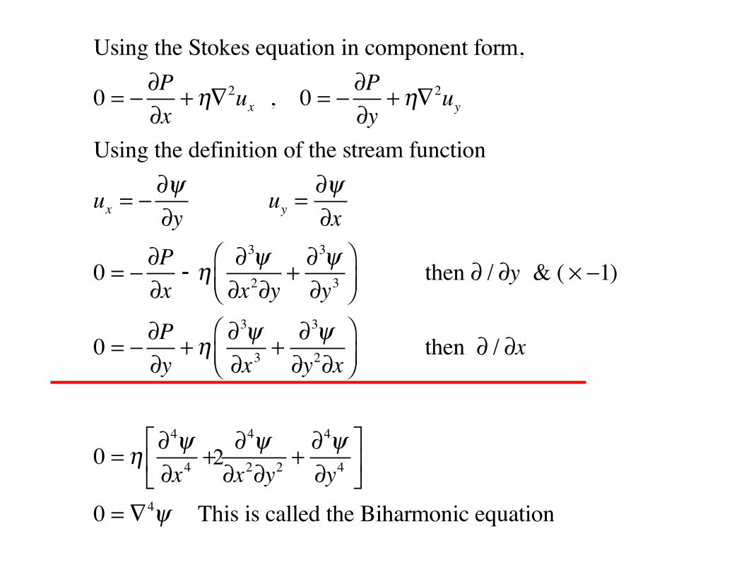
Using the Stokes equation in component form,

0 = −∂P∂x

+η∇2ux , 0 = −∂P∂y

+η∇2uy

Using the definition of the stream function

ux = −∂ψ∂y

uy =∂ψ∂x

0 = −∂P∂x

+η ∂3ψ∂x2∂y

+∂3ψ∂y3

⎛⎝⎜

⎞⎠⎟

then ∂ / ∂y & ( × −1)

0 = −∂P∂y

+η ∂3ψ∂x3 +

∂3ψ∂y2∂x

⎛⎝⎜

⎞⎠⎟

then ∂ / ∂x

0 = η ∂4ψ∂x4 +

∂4ψ∂x2∂y2 +

∂4ψ∂y4

⎡

⎣⎢

⎤

⎦⎥

0 = ∇4ψ This is called the Biharmonic equation

-

2

If we didn't assume ∂ρ / ∂x = 0, then

η∇4ψ = −g∂ρ∂x

The flow is generated by lateral variations in density.

The equation reduces to a balance between a gravitationalbuoyancy force and viscous resistance.

Response of a semi-infinite half-space to a periodic load (all details are given in section 6-10 in Turcotte and Schubert

y

w

g

ρ2

ρ1

Δρ = ρ1 − ρ2

Solve ∇4ψ = 0, the biharmonic equation

w = wo cos 2π xλ

initial condition.

w = vertical displacement ("topography").

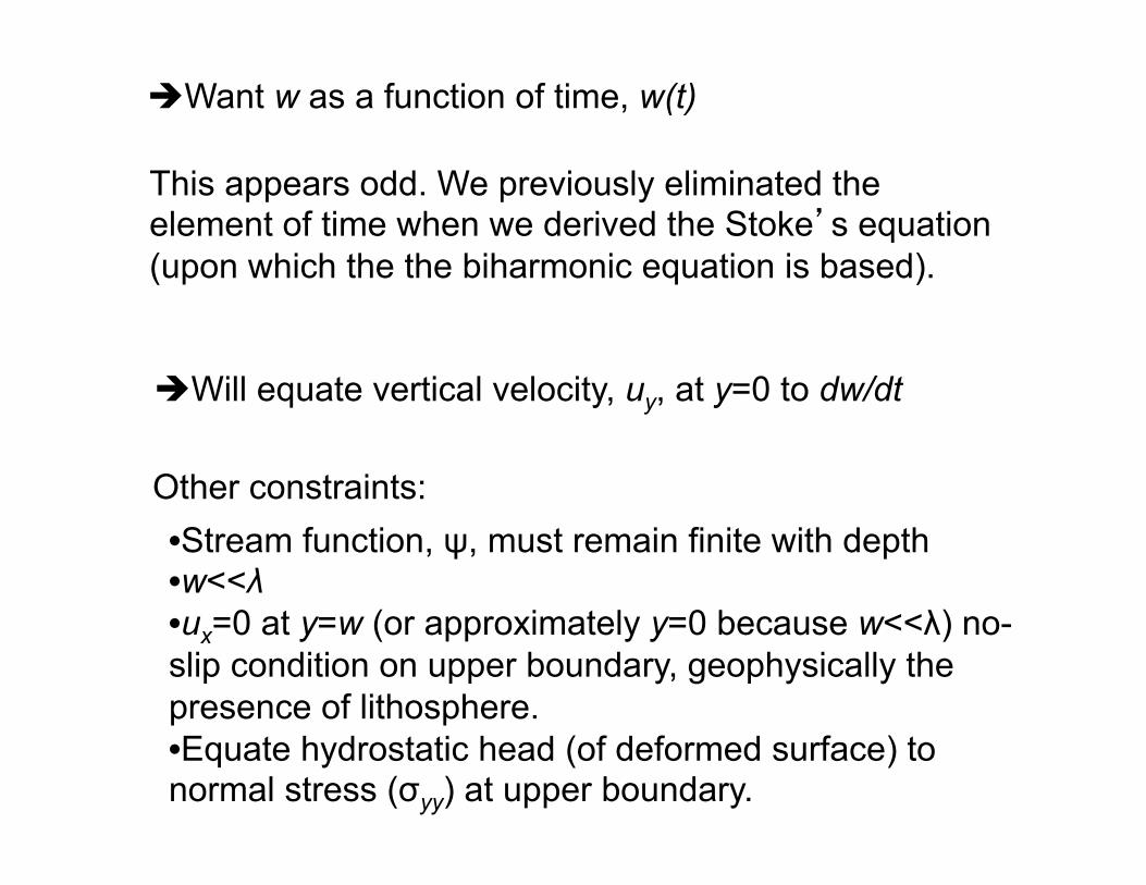
Want w as a function of time, w(t)

This appears odd. We previously eliminated the element of time when we derived the Stoke’s equation (upon which the the biharmonic equation is based).

Will equate vertical velocity, uy, at y=0 to dw/dt

Other constraints: • Stream function, ψ, must remain finite with depth • w<<λ • ux=0 at y=w (or approximately y=0 because w<<λ) no-slip condition on upper boundary, geophysically the presence of lithosphere. • Equate hydrostatic head (of deformed surface) to normal stress (σyy) at upper boundary.

To solve ∇4 = 0 use separation of variablesψ = X(x)Y (y)

Guess ψ = A 'sin 2π xλ

+ B 'cos 2π xλ

⎡⎣⎢

⎤⎦⎥Y (y)

...Using the fact that the solution must be bounded as y→∞ andthe no-slip boundary condition:

uy = A2πλ

⎛⎝⎜

⎞⎠⎟

cos 2πλx⎛

⎝⎜⎞⎠⎟e−2π y /λ 1+ 2π

λy⎛

⎝⎜⎞⎠⎟

�

∇4ψ = 0

To evaluate A Equate hydrostatic head, − ρgw, to the total normal stressat the upper boundary of the fluid half-space. From the stresstensor:

σ yy = p −τ yy = p − 2η∂uy∂y

Set σ yy = −ρgw (notice that w appears for the first time).Find p by setting up a horizontal balance, e.g.0 = −∇p +η2ux Then integrate one

p = 2ηA 2πλ

⎛⎝⎜

⎞⎠⎟

2

cos 2πλx⎛

⎝⎜⎞⎠⎟ y=0

⇒−ρgw(x) = p

w(x) y=0 = − 1ρg

⎛⎝⎜

⎞⎠⎟

2ηA 2πλ

⎛⎝⎜

⎞⎠⎟

2

cos 2πλx⎛

⎝⎜⎞⎠⎟

⇒ put A in terms of w

�

0 = −∇p + η∇2ux

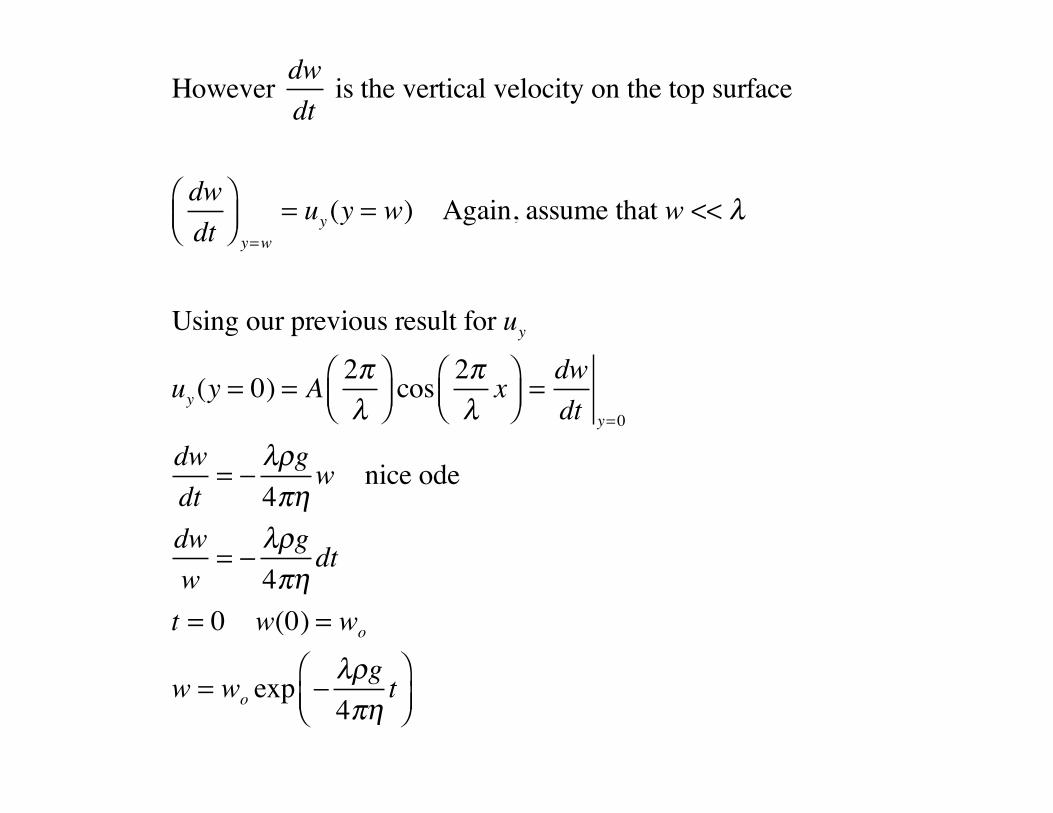
However dwdt

is the vertical velocity on the top surface

dwdt

⎛⎝⎜

⎞⎠⎟ y=w

= uy (y = w) Again, assume that w << λ

Using our previous result for uy

uy (y = 0) = A 2πλ

⎛⎝⎜

⎞⎠⎟

cos 2πλx⎛

⎝⎜⎞⎠⎟=dwdt y=0

dwdt

= −λρg4πη

w nice ode

dww

= −λρg4πη

dt

t = 0 w(0) = wo

w = wo exp −λρg4πη

t⎛⎝⎜

⎞⎠⎟

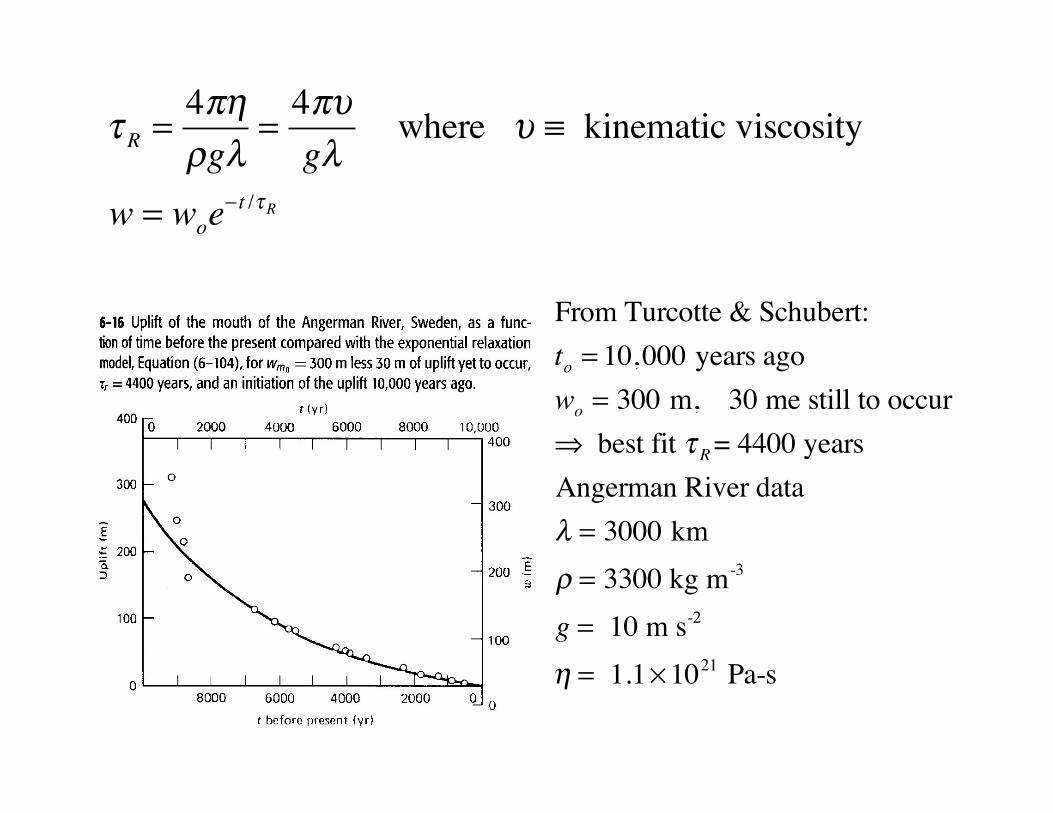
τ R =4πηρgλ

=4πυgλ

where υ ≡ kinematic viscosity

w = woe− t /τR

From Turcotte & Schubert:to = 10,000 years agowo = 300 m, 30 me still to occur⇒ best fit τ R= 4400 yearsAngerman River dataλ = 3000 kmρ = 3300 kg m-3

g = 10 m s-2

η = 1.1×1021 Pa-s

Why is there an inverse relation between relaxation time and wavelength?

τ R =4πηρgλ

τ R ∝hh

hh=

4πηρgλ

ρgh = 4πηhλ

stress=(viscosity) × (strain-rate)

Practical: Have you ever poured honey back into a bowl of Honey? First there is a wide ridge, but after time there is a Sharp line that persists for a long time.

Cathles [1975]

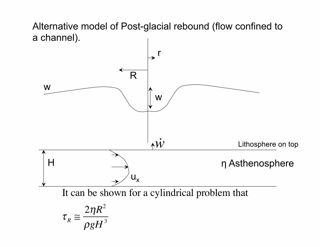
Alternative model of Post-glacial rebound (flow confined to a channel).

w

r

R

w

Lithosphere on top

η Asthenosphere H ux

w

It can be shown for a cylindrical problem that

τ R ≅2ηR2

ρgH 3

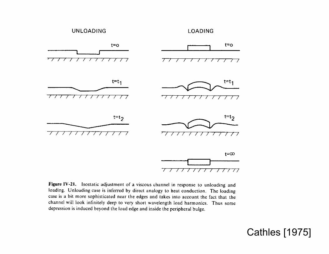
Cathles [1975]

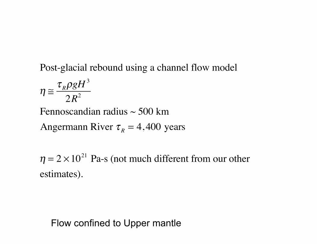
Post-glacial rebound using a channel flow model

η ≅τ RρgH

3

2R2

Fennoscandian radius ~ 500 kmAngermann River τ R = 4,400 years

η = 2 ×1021 Pa-s (not much different from our otherestimates).

Flow confined to Upper mantle

Cathles [1975]

RSLs at different Distances from the Ice Cap

Peltier

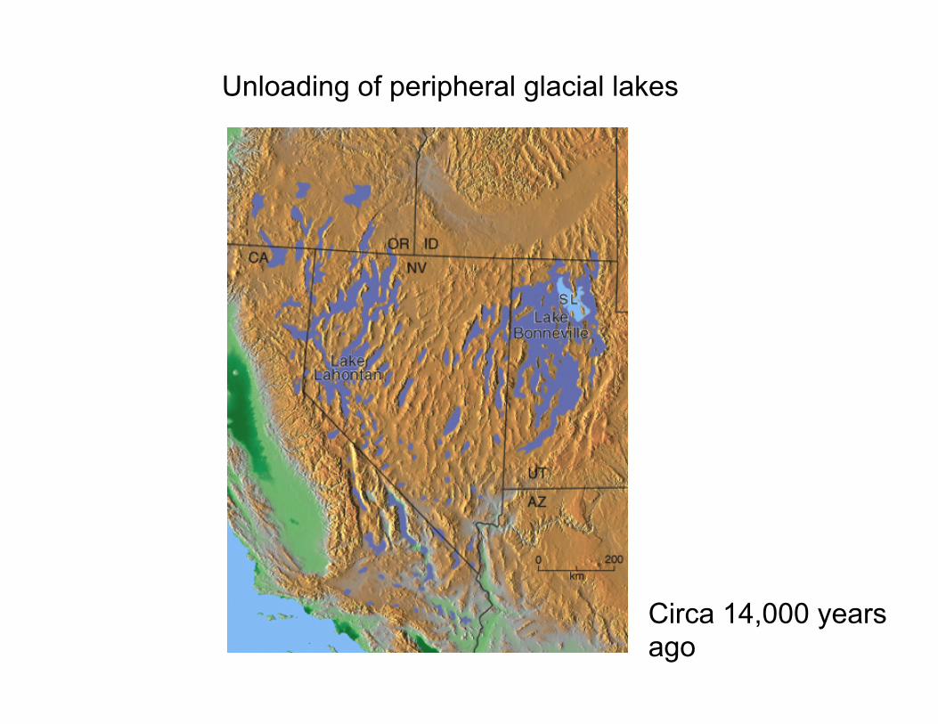
Unloading of peripheral glacial lakes

Circa 14,000 years ago

Crittenden [1963]: “Shorelines [of Lake Bonneville], originally level are domed upward about 64 meters in the center of the basin, showing that during both loading and subsequent unloading, the earth reached a high degree…of isostatic adjustment. To attain this degree of compensation the isostatic anomaly created during loading or unloading must be reduced to 1/e of its initial value in about 4,000 years” Now this time-scale is about the same as Fennoscandia, but Bonneville has ~1/10 the diameter Channel Flow

τ R =2ηR2

ρgH 3 Note the strong trade-off between H and η

ηB

ηF

=RFRB

⎛⎝⎜

⎞⎠⎟

2HB

HF

⎛⎝⎜

⎞⎠⎟

3

= 100 HB

HF

⎛⎝⎜

⎞⎠⎟

3

HB = 70 kmHF = 700 kmηF ~ 1021 Pa-s ηB ~ 1020 Pa-s (Cathles: 4x1019 Pa-s)

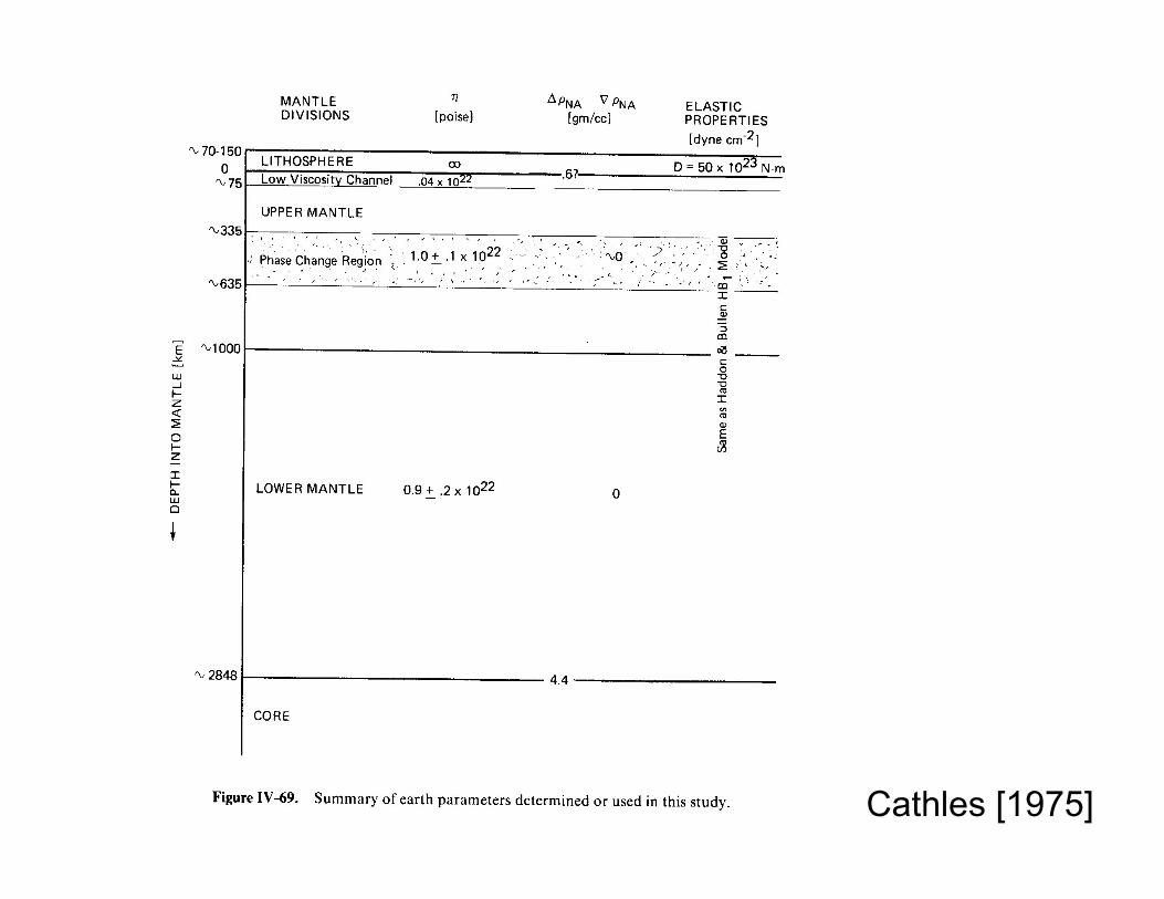
Cathles [1975]

Except for a ‘low viscosity channel’ beneath the lithosphere, does the mantle have a uniform, 1021 Pas-s, viscosity as Cathles [1975] argues?

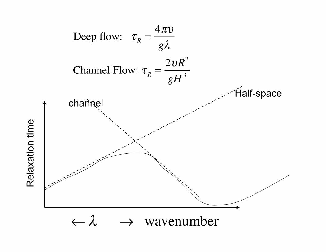
Deep flow: τ R =4πυgλ

Channel Flow: τ R =2υR2

gH 3

←λ → wavenumber

Rel

axat

ion

time

Half-space channel

Models like this can give the appropriate relaxation spectrum

depth

viscosity

Weak upper mantle

Can the “relaxation spectra” be observed? (I.e. relaxation time versus wavelength) Several attempts over the years. Most recent, is to look at the localization of gravity (spectrogram of the gravity)

‘Spectogram’ of gravity field: Hudson’s Bay is A unique feature of the gravity field.

Simons & Hager [1997]

1.  Gravity is highly correlated with former ice caps

2.  Use a model for the time load (such as ICE-1)

3.  Isostatically compensate ice-load (mantle viscosity is not needed)

4.  Remove ice load ‘instantly’ and calculate gravity

5.  Correlate the model gravity with observed gravity versus wavelength, Fl

Simons and Hager [1997]

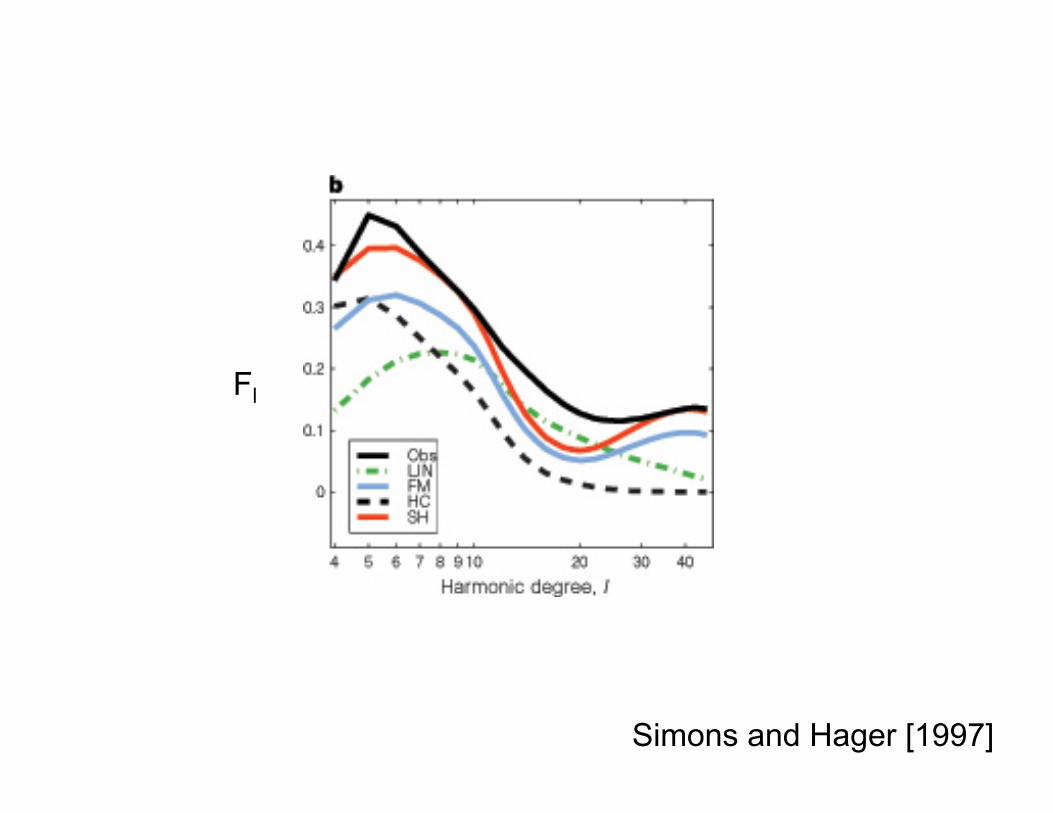
Fl

Simons and Hager [1997]

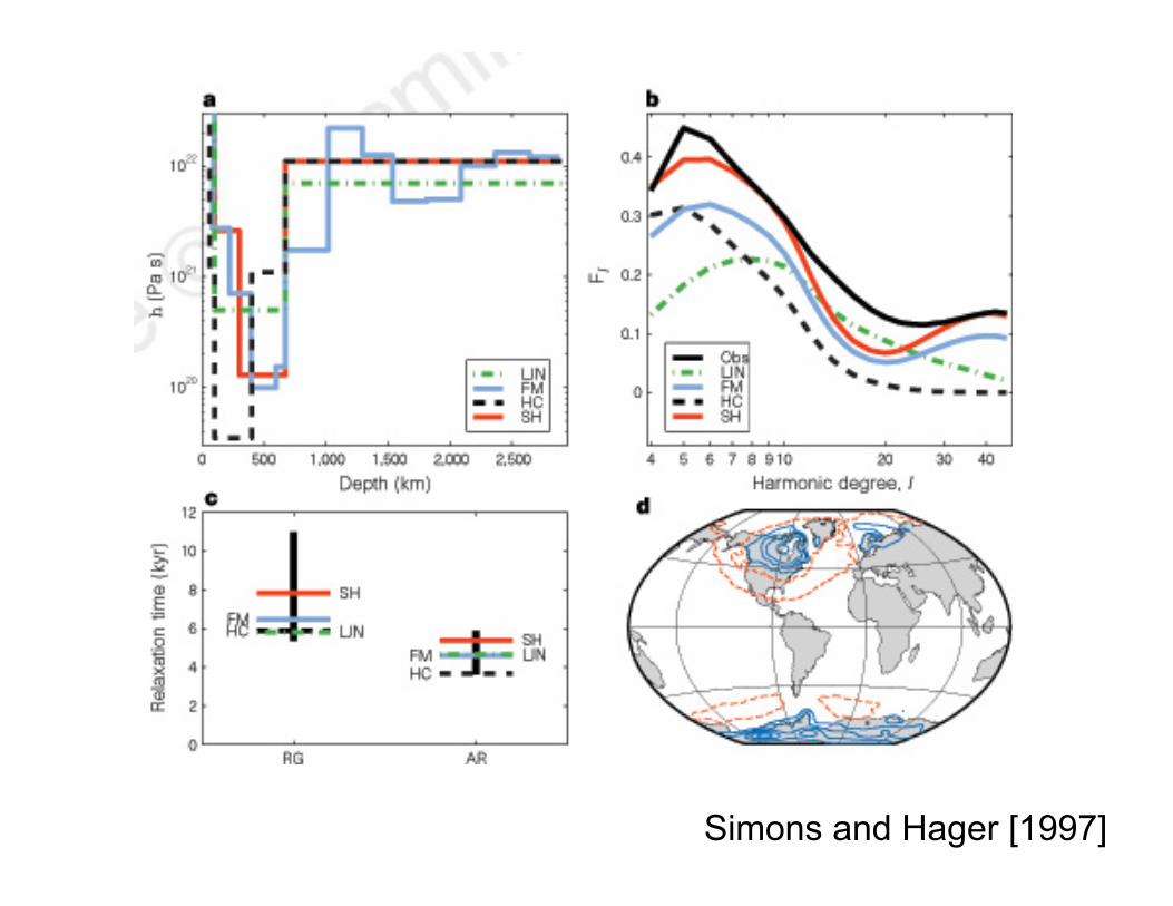
Simons and Hager [1997]

3-D Velocities from present Day GPS

Milne et al. [2001]

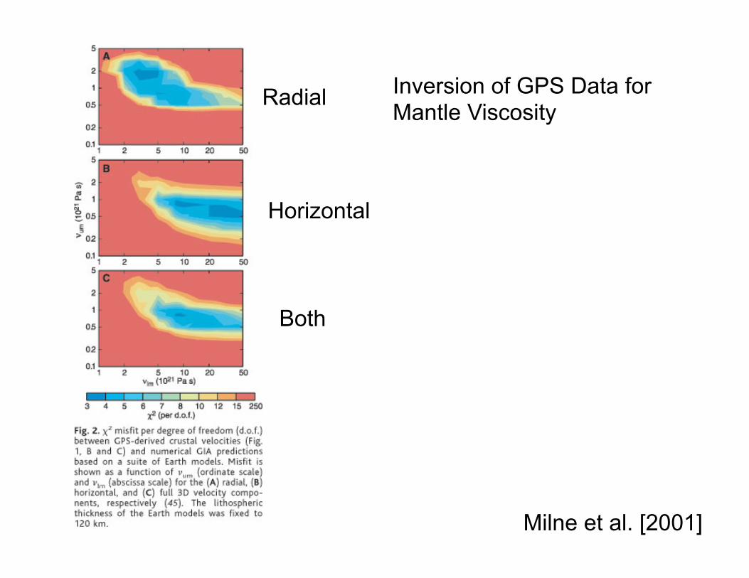
Inversion of GPS Data for Mantle Viscosity

Milne et al. [2001]

Radial

Horizontal

Both

Secular change in gravity from GRACE (In units of µGal/yr)

)

Homogeneous mantle models fit GRACE & RSL have viscosities of 1.4 to 2.3 X 1021 Pa s

Paulson et al [2007]

Viscosity Structure Used in Spherical FEM model of post-glacial rebound

Paulson, et al. [2005]

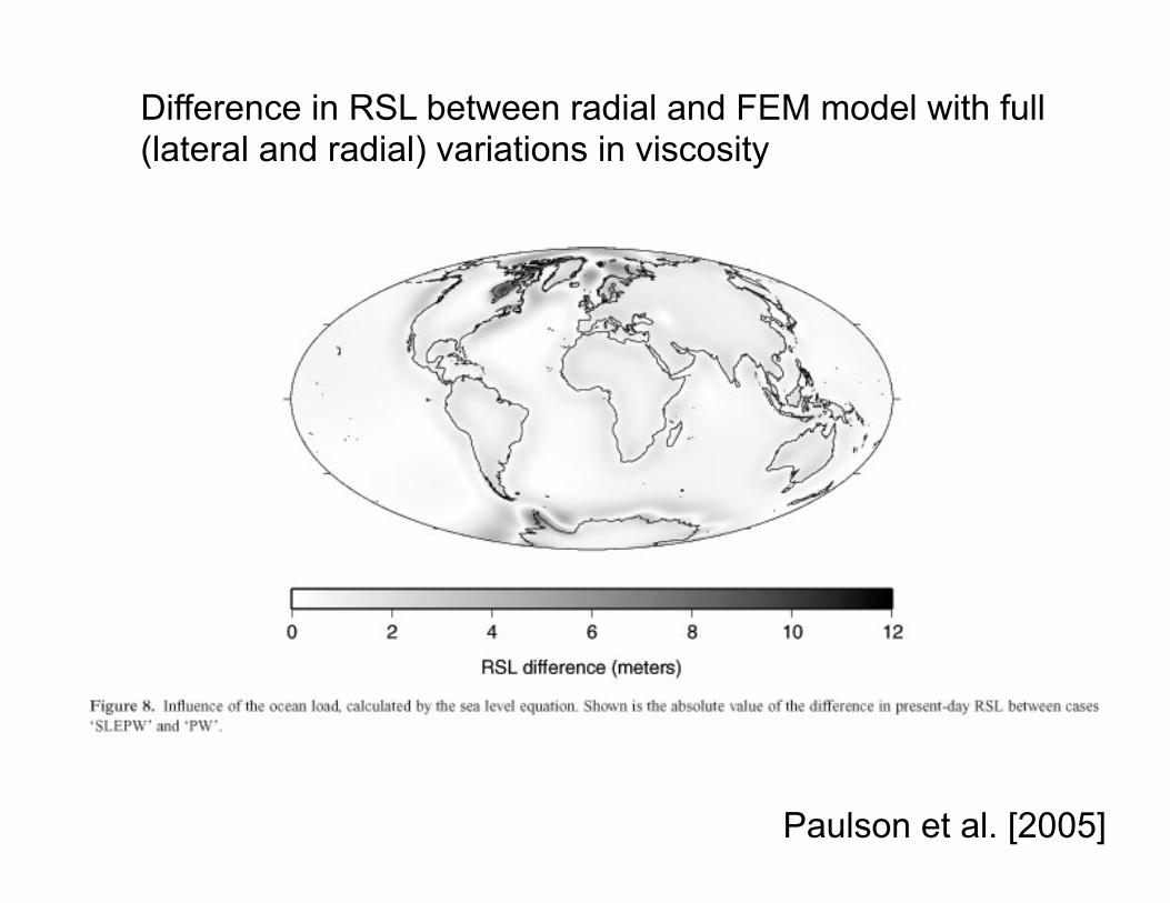
Difference in RSL between radial and FEM model with full (lateral and radial) variations in viscosity

Paulson et al. [2005]