7 slides

Dr. Rakhesh Singh Kshetrimayum

7. Transmission line analysis

Dr. Rakhesh Singh Kshetrimayum

5/20/20131 Electromagnetic Field Theory by R. S. Kshetrimayum

7.1 Introduction Transmission line analysis

Introduction

Wave equation

Lossless line

High reactance effect

Telegrapher’s equations

Lossy line Smith chart

Ideal

Terminated

5/20/2013Electromagnetic Field Theory by R. S. Kshetrimayum2

Line junction

Distributed element concept Fig. 7.1 Transmission line

λ/4 transformerLine impedance

Terminated

IdealImpedance

Admittance

Radiation effect

Sizeeffect

7.1 IntroductionHigh reactance effect

Consider a 10-V ac source is connected to a 50 Ω load by a small copper wire of 1 mm radius

Assume that the dc resistance of the wire is R=1m Ω and inductance of L=0.1 µH


inductance of L=0.1 µH

At 10 GHz, inductive reactance is jXL=jωL≈6283 Ω and hence all the ac signal will die out in the wire itself

The load will not receive any signal

Hence we need special devices which will take these signals from the source to the load

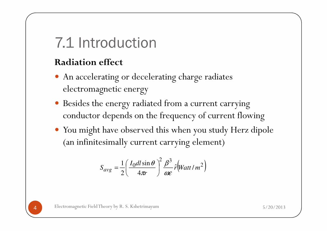
7.1 IntroductionRadiation effect

An accelerating or decelerating charge radiates electromagnetic energy

Besides the energy radiated from a current carrying conductor depends on the frequency of current flowing


conductor depends on the frequency of current flowing

You might have observed this when you study Herz dipole (an infinitesimally current carrying element)

( )232

0 /ˆ4

sin

2

1mWattr

r

dlISavg

ωε

β

π

θ

=

7.1 Introduction Hence the radiation power loss is directly proportional to the square of the frequency of the ac current flowing

So there will be high loss of power

We definitely cannot use open wires for transferring energy or signal


or signal

7.1 Introduction7.1.1 Introduction

What is a transmission line?

A structure, which can guide electrical energy from one point to another

Generally, a transmission line is a two parallel conductor system


a two parallel conductor system one end of which is connected to a source and the other end is connected to a load

Examples: coaxial cables waveguides microstrip lines

7.1 Introduction


Fig. 7.2 (a) Transmission lines examples (b) General transmission line structure

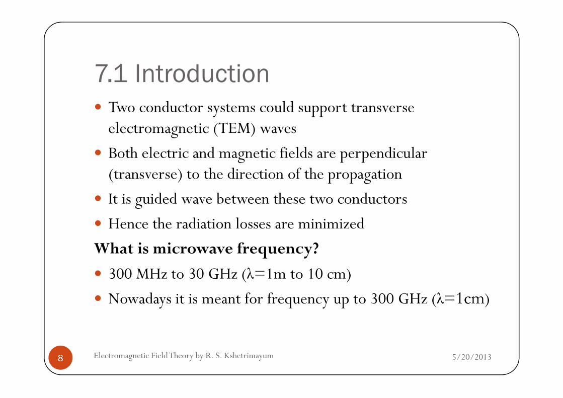
7.1 Introduction Two conductor systems could support transverse electromagnetic (TEM) waves

Both electric and magnetic fields are perpendicular (transverse) to the direction of the propagation

It is guided wave between these two conductors


It is guided wave between these two conductors

Hence the radiation losses are minimized

What is microwave frequency?

300 MHz to 30 GHz (λ=1m to 10 cm)

Nowadays it is meant for frequency up to 300 GHz (λ=1cm)

7.1 IntroductionSize effect

Size of commonly used lump elements like capacitor, inductor and resistor are of the order of cm

Now this size is comparable to the microwave wavelength

Hence the phase βl=(2πf/c)l of the electrical signal might


Hence the phase βl=(2πf/c)l of the electrical signal might vary along the length of the device

For instance, consider a parallel plate capacitor

We assume capacitor conductor plate is an equipotentialsurface

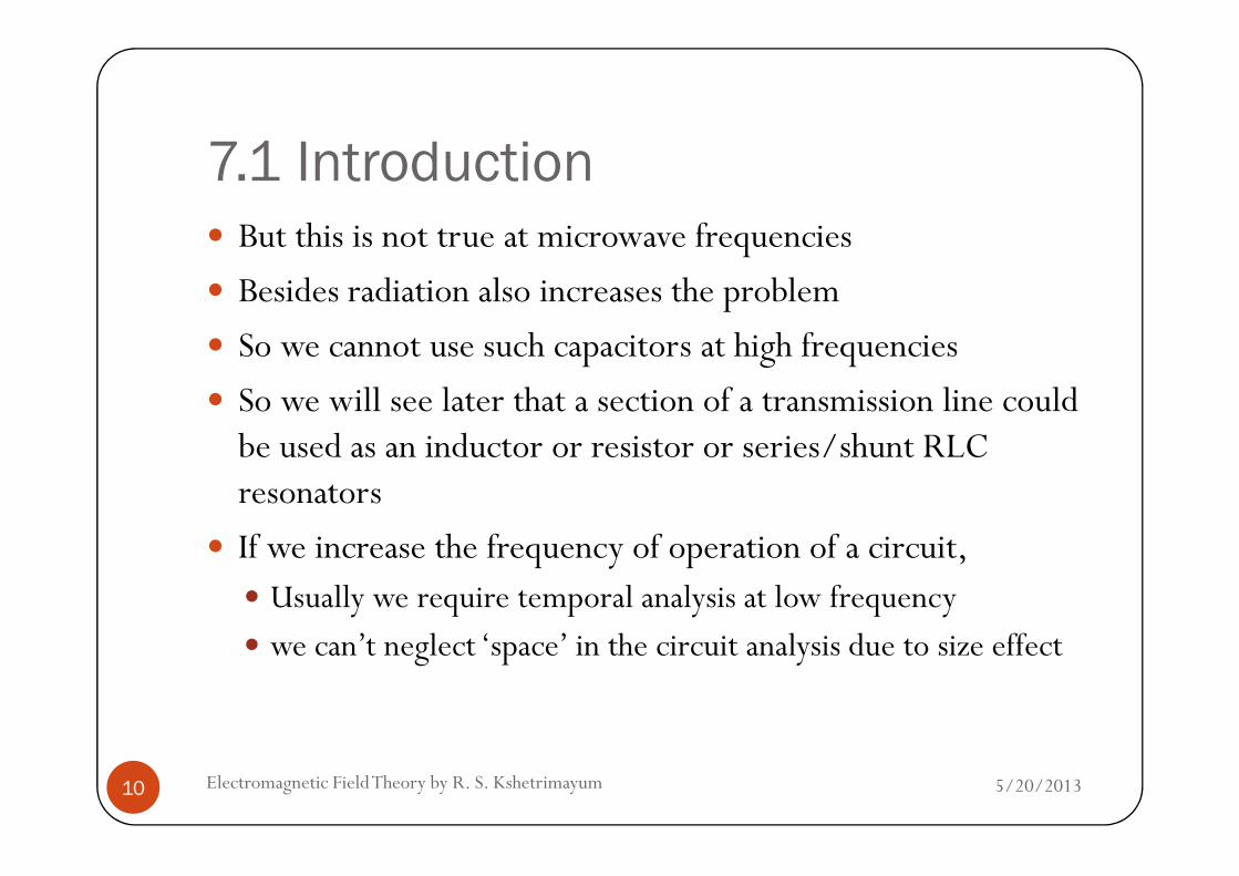
7.1 Introduction But this is not true at microwave frequencies

Besides radiation also increases the problem

So we cannot use such capacitors at high frequencies

So we will see later that a section of a transmission line could be used as an inductor or resistor or series/shunt RLC


be used as an inductor or resistor or series/shunt RLC resonators

If we increase the frequency of operation of a circuit, Usually we require temporal analysis at low frequency

we can’t neglect ‘space’ in the circuit analysis due to size effect

7.1 Introduction7.1.2 Causal effect

What is causal effect?

EM wave requires a finite time to travel along an electrical circuit

Since no EM wave can travel with infinite velocity


Since no EM wave can travel with infinite velocity (What is the maximum speed?)

A finite time delay between the 'cause' and the ‘effect’ Also known as the causal effect in physics

When is this effect important?

7.1 Introduction If the time period of the EM wave or signal

(T=1/f) >> the transit time (tr), we may ignore this effect

1r

l vT t l l

f v fλ>> ⇒ >> ⇒ >> ⇒ >>


Causal effect becomes important when the length of the line (l) becomes comparable to the wavelength (λ)

As the frequency increases, the wavelength reduces, and

the Causal effect becomes more evident

7.1 Introduction7.1.3 Distributed vs lumped elements To overcome the effect of transit time or causality or size effect (more appropriate to use), one can chop off the transmission line into small sections

such that for each section, this causality effect is minuscule

At high frequencies,


At high frequencies, the circuit elements cannot be defined for the whole transmission line instead it has to be defined for a unit length of the line

The circuit elements are not located at a point of the line but are distributed all along the length

7.1 Introduction Analysis of a transmission lines must be carried out using

the concept of distributed elements not as

lumped elements

as we used to do from our previous circuit analysis at the low frequencies


frequencies

But, we can still employ lump element analysis of transmission lines by chopping off small sections of the line

so that the Causal effect is negligible in the chopped off sections

7.2 Telegrapher’s equations 7.2.1 Lumped element circuit model

Per unit length parameters: L=Series inductance per unit length

C=Shunt capacitance per unit length

R=Series resistance per unit length


R=Series resistance per unit length

G= Shunt conductance per unit length

7.2 Telegrapher’s equations

z∆


zR∆ zL∆

zG∆zC∆)t,z(I),t,z(V

)t,zz(I),t,zz(V ∆+∆+

Fig. 7.3 (a) Sub-section of length ∆z of a general transmission line and its (b) lumped element equivalent circuit

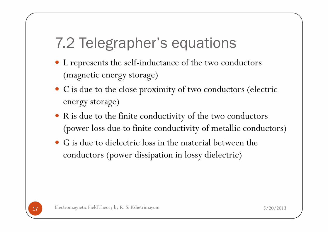
7.2 Telegrapher’s equations L represents the self-inductance of the two conductors (magnetic energy storage)

C is due to the close proximity of two conductors (electric energy storage)

R is due to the finite conductivity of the two conductors


R is due to the finite conductivity of the two conductors (power loss due to finite conductivity of metallic conductors)

G is due to dielectric loss in the material between the conductors (power dissipation in lossy dielectric)

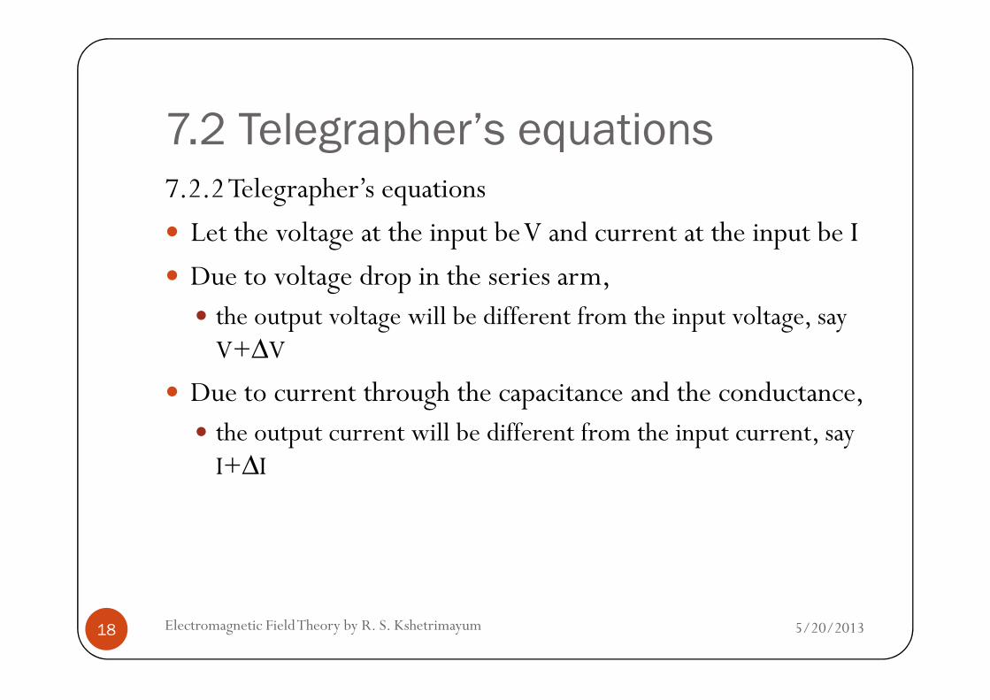
7.2 Telegrapher’s equations 7.2.2 Telegrapher’s equations

Let the voltage at the input be V and current at the input be I

Due to voltage drop in the series arm, the output voltage will be different from the input voltage, say V+∆V


V+∆V

Due to current through the capacitance and the conductance, the output current will be different from the input current, say I+∆I

7.2 Telegrapher’s equations Applying Kirchoff’s voltage law (KVL) and Kirchoff’s current law (KCL)

i(z, t)v(z, t) R zi(z, t) L z v(z z, t) 0

t

δ− ∆ − ∆ − + ∆ =

δ


v(z z, t)i(z, t) G zv(z z, t) C z i(z z, t) 0

t

δ + ∆− ∆ + ∆ − ∆ − + ∆ =

δ

7.2 Telegrapher’s equations Dividing the above two equations by Δz and taking the limit

Δz 0 (What is its implications?)

v(z, t) i(z, t)Ri(z, t) L

z t

δ δ= − −

δ δ


z tδ δ

i(z, t) v(z, t)Gv(z, t) C

z t

δ δ= − −

δ δ

Telegrapher’s Equations

7.2 Telegrapher’s equations 7.2.3 Wave propagation

For time-harmonic signals, telegrapher’s equation reduces to

dV(z)(R j L)I(z)

dz= − + ω


dz

( )-( ) ( )

dI zG j C V z

dzω= +

7.2 Telegrapher’s equations It is similar to Maxwell’s curl equations, hence, we can get wave equations

0V(z)γdz

V(z)d 2

2

2

=−


0I(z)γdz

I(z)d 2

2

2

=−

( )( )j R j L G j Cγ α β ω ω= + = + +

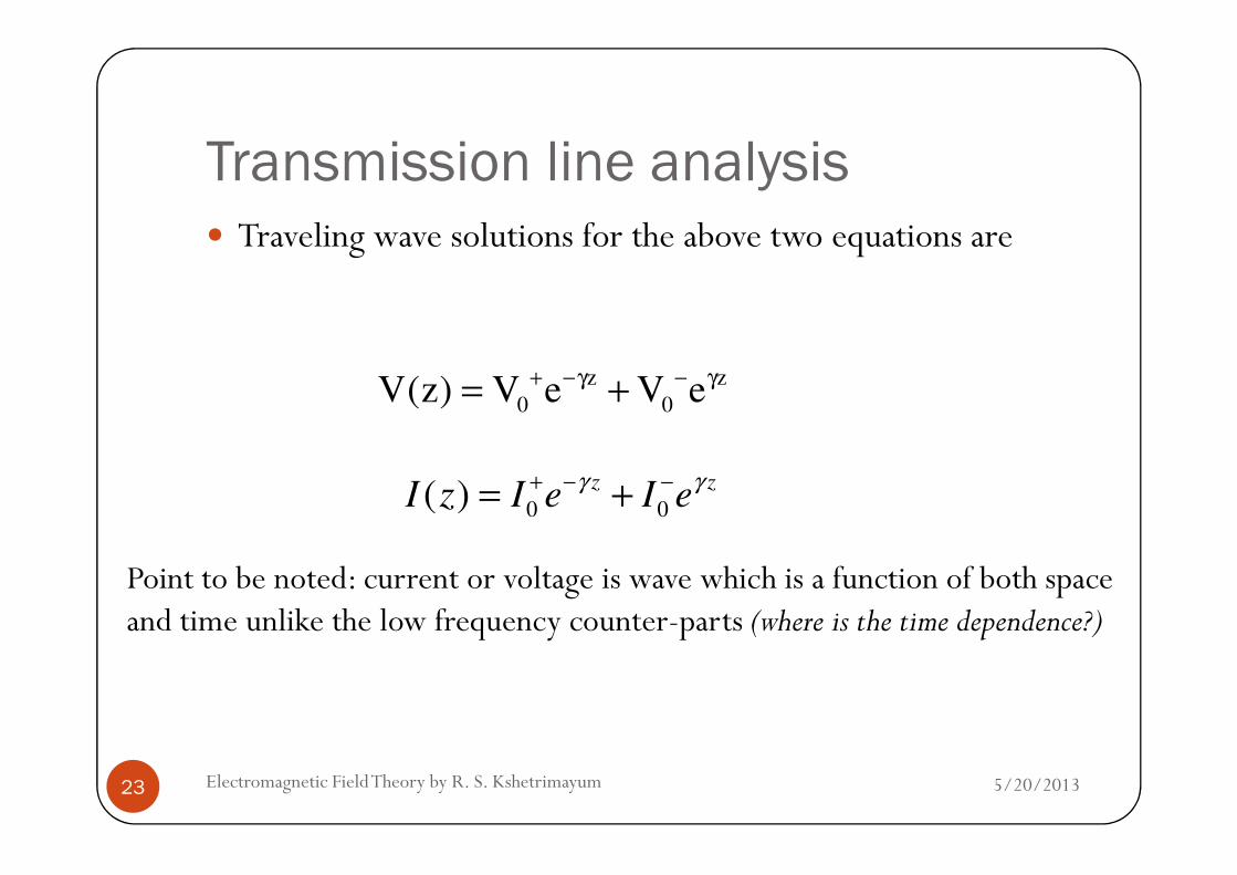
Transmission line analysis Traveling wave solutions for the above two equations are

z z

0 0V(z) V e V e+ −γ − γ= +


0 0( ) z zI z I e I e

γ γ+ − −= +

Point to be noted: current or voltage is wave which is a function of both space and time unlike the low frequency counter-parts (where is the time dependence?)

7.2 Telegrapher’s equations Physical interpretations

Wave phase has two components: time phase (ωt) and

space phase (βz)

Since βz is the phase of the wave as function of z,


Since βz is the phase of the wave as function of z, β represents phase change per unit length of the transmission line for a traveling wave

phase constant (unit is radians per meter)

)φzβtωcos(eVeeeVReeeVRe zαzβjtωjzαφjzβjtωjzα +−== −+−−+−−+

7.2 Telegrapher’s equations For a positive α, the amplitude exponentially decreases as a function of z

α represents attenuation of the wave on the transmission line

attenuation constant of the line (unit is Nepers per meter, 1 Neper= 8.68dB)

zV e

α+ −


1 Neper= 8.68dB)z z

0 0I(z) V e V eR j L

+ −γ − γγ = − + ω

0

R j L R j LZ

G j C

+ ω + ω= =

γ + ω

0 00

0 0

V VZ

I I

+ −

+ −= = −

7.2 Telegrapher’s equations The characteristic impedance Z0 of a transmission line is

defined as the ratio of positively traveling voltage wave to current wave at any point on the line

Now for a wave the distance over which the phase changes by 2H is called the wavelength 'λ’


2H is called the wavelength 'λ’

phase change per unit length β=2H/λ

p

2 fv f

π ω= λ = =

β β

7.3 Lossless line7.3.1 Ideal lossless line

zL∆

zC∆)t,z(I),t,z(V)t,zz(I),t,zz(V ∆+∆+


)t,z(I),t,z(V

Fig. 7.4 Lumped element equivalent circuit of a sub-section oflength ∆z of a lossless transmission line (R=G=0)

7.3 Lossless line

j j LCγ = α + β = ω LCβ = ω 0α =

LZ =

j z j zV(z) V e V e+ − β − β= +


0ZC

= 0 0V(z) V e V e= +

j z j z0 0

0 0

V VI(z) e e

Z Z

+ −

− β β= −2 2

LC

π πλ = =

β ω

p

1v

LC LC

ω ω= = =

β ω

7.3 Lossless line7.3.2 Terminated lossless lines

β,Z


β,Z0

Fig. 7.4 (b) A lossless transmission line terminated with load impedance ZL

7.3 Lossless line7.3.3 Reflection coefficient

At the load, z=0,

( )( ) 0

ooL Z

VV0VZ

−+

−+ +== 0L0 ZZV −

=Γ=+

−


( ) 0

oo

ooL Z

VV0IZ

−+ −==

0L

0L

0

0

ZZV +=Γ=

+

( ) ( )zβjzβj0 eeVzV Γ+= −+ ( ) ( )zβjzβj

0

0 eeZ

VzI Γ−= −

+

z = −l ( ) ( ) lj

lj

lj

eeV

eVl

β

β

β2

0

0 0 −

++

−−

Γ==Γ ( )0

00ZZ

ZZ

L

L

+

−=Γ

7.3 Lossless line7.3.4 Power flow and return loss

Time average power flow along the line at the point z,

( ) ( ) 2

* 20 * 2 * 21 1Re Re 1

2 2

z z

avg

VS V z I z e e

Z

β β

+

− − = = − Γ + Γ − Γ


02 2

avgZ

2

20

0

11

2avg

VS

Z

+

= − Γ

7.3 Lossless line When the load is mismatched,

not all of the available power from the generator is delivered to the load,

this “loss” is called Return loss (RL) and is defined in dB as

7.3.5 Standing wave ratio (SWR)


7.3.5 Standing wave ratio (SWR)

Γ−= log20RL

( ) 2

0 1 j zV z V e

β+= + Γ2 j ze 1β = Γ+= + 10max VV

2 j ze 1β = − Γ−= + 10min VVΓ−

Γ+==

1

1

min

max

V

VVSWR

7.3 Lossless lineWhat is BW?

For acceptable value of VSWR = 2 within the operating frequency region of a device also known as bandwidth (BW)

54.93

1log20;

3

1

12

12

1

1=

−==

+

−=

+

−=Γ RL

VSWR

VSWR


Return loss (RL) should be higher than 9.54, which is approximately 10 dB

RL ≥10 dB has become an acceptable definition for BW of many devices

33121 ++VSWR

7.3 Lossless line

max

min

IISWR

I=

( )2max maxV I

PSWR PSWR ISWR VSWRV I

= = × =


For VSWR=2, only 89% of the incident power reaches the load

min minV I

( )( )

22

2

1 41 1

1 1

i rL

i i

P PP VSWR VSWR

P P VSWR VSWR

− − = = − Γ = − =

+ +

7.3 Lossless line

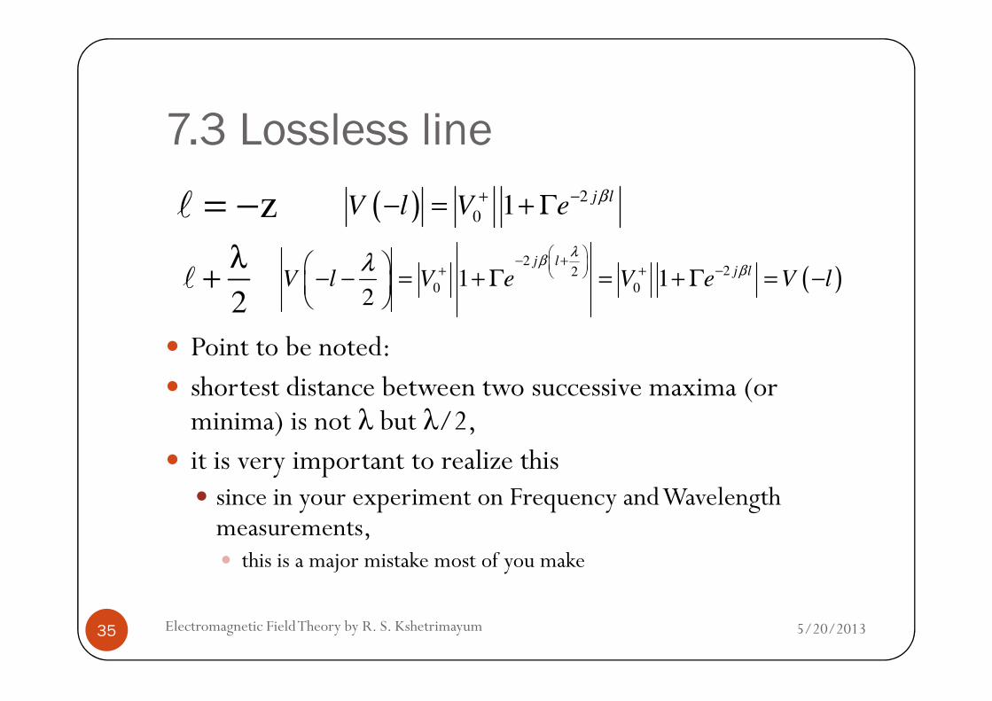
Point to be noted:

z= −l ( ) 2

01 j l

V l V eβ+ −− = + Γ

2

λ+l ( )

222

0 01 12

j lj l

V l V e V e V l

λβ

βλ

− + + + − − − = + Γ = + Γ = −


Point to be noted: shortest distance between two successive maxima (or minima) is not λ but λ/2,

it is very important to realize this since in your experiment on Frequency and Wavelength measurements, this is a major mistake most of you make

7.3 Lossless line

the distance between adjacent maximum and minimum is λ/4

7.3.6 Transmission line impedance equation

4

λ+l

224

0 01 14

j lj l

V l V e V e

λβ

βλ

− + + + − − − = + Γ = − Γ


7.3.6 Transmission line impedance equation

A certain value of load impedance at the end of a particular transmission line is transformed into another value of impedance at the input of the line

impedance transformer

7.3 Lossless line Transmission line impedance equation

( )( )

0

0 0

0 0

0 0

j l j lL

j l j l

L

in j l j l

j l j lL

Z Ze e

V e e Z ZV lZ Z Z

I l V e e Z Ze e

β ββ β

β ββ β

−

+ −

+ −

−

−+ + Γ +− = = =

− − Γ − −


( ) ( )

( ) ( )

( ) ( )

0

0

00 0

0 0

0 0

j l j lL

L

j l j l j l j lj l j lLL L

j l j l

L L

e eZ Z

Z e e Z e eZ Z e Z Z eZ Z

Z Z e Z Z e Z

β β β ββ β

β β

− −−

−

− +

+ + − + + − = = + − − ( ) ( )

( ) ( )

( ) ( )

0

0 00 0

00

cos sin tan( )

tan( )cos sin

j l j l j l j l

L

L L

LL

e e Z e e

Z l jZ l Z jZZ Z

Z jZZ l jZ l

β β β β

β β β

ββ β

− − + + −

+ + = =+ +

l

l

7.3 Lossless lineFig. 7.5 Transmission line impedance


β,Z0

inZ

7.3 Lossless line7.3.7 Quarter-wave transformer

n4 2

λ λ= +l

( )

2 2n n n

4 2 4 2 2

tan tan n2

λ λ π λ π λ πβ = β + β = + = + π

λ λ

π ⇒ β = + π = ∞

l

l

2Z jZ tan( ) jZ tan( ) Z+ β β

0 L inZ Z Z=


How to do impedance matching for a complex load using quarter-wave transformer?

2

L 0 0 0in 0 0

0 L L L

Z jZ tan( ) jZ tan( ) ZZ Z Z

Z jZ tan( ) jZ tan( ) Z

+ β β⇒ = = =

+ β β

l l

l l

7.3 Lossless line7.3.8 Special cases of lossless terminated lines

Terminated in a short circuit

Terminated in open circuit

sc L 0in 0 0

0 L

Z jZ tan( )Z Z jZ tan( )

Z jZ tan( )

+ β= = β

+ β

ll

l


Terminated in open circuit

Terminated with matched load

oc L 0in 0 0

0 L

Z jZ tan( )Z Z jZ cot( )

Z jZ tan( )

+ β= = − β

+ β

ll

l

0ZZ

ZZ

00

00 =+

−=Γ

7.3 Lossless line Another important observation is that

if we measure open and

short circuit input impedances

of a lossless transmission line and


multiply those two values and

take the square root

what we have is the characteristic impedance of the line (one of the methods for finding the characteristic impedance of a given line in laboratory)

7.3 Lossless line7.3.9 Reflection and transmission at the transmission line junction

Γ τ


Fig. 7.7 Junction of two transmission line with different characteristic impedance

7.3 Lossless line For z<0,

characteristic impedance Z0;

z>0, characteristic impedance Z1 and

the junction of the two transmission lines is at z=0

At the junction,


At the junction, looking from z<0 towards the right, it sees an infinite transmission line of characteristic impedance Z1 and

hence it is equivalent to ZL=Z1 for the transmission line z<0

Assuming ζ is the transmission coefficient and IL is insertion loss in dB

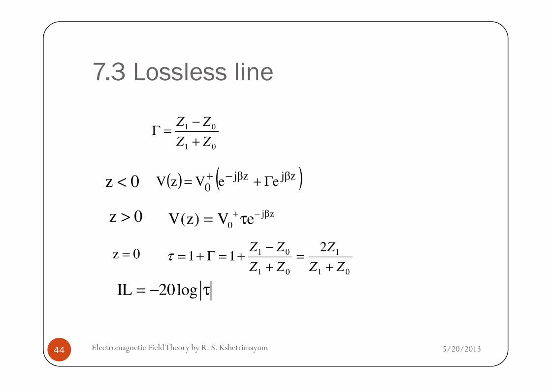
7.3 Lossless line

01

01

ZZ

ZZ

+

−=Γ

z 0< ( ) ( )zβjzβj0

eeVzV Γ+= −+


z 0> j z

0V(z) V e+ − β= τ

z 0=01

1

01

01 211

ZZ

Z

ZZ

ZZ

+=

+

−+=Γ+=τ

IL 20log= − τ

7.4 Lossy lines One type of metal loss is I2R loss

In transmission lines, the resistance of the conductors is never equal to zero

except for superconductors

Whenever current flows through one of these conductors,


Whenever current flows through one of these conductors, some energy is dissipated in the form of heat

7.4 Lossy lines Another type of loss is due to skin effect

Current in the center of the wire becomes smaller and

most of the electron flows on the wire surface

When the frequency applied is in the GHz range, the electron movement in the center is so small


the electron movement in the center is so small

that the center of the wire could be removed without any noticeable effect on the current

7.4 Lossy lines Note that the effective cross-sectional area

decreases as the frequency increases

Since resistance is inversely proportional to the cross-sectional area (R=ρl/A),

the resistance will increase as the frequency is increased


the resistance will increase as the frequency is increased

Also, since power loss increases as resistance increases,

power losses increase with an increase in frequency

because of the skin effect

7.4 Lossy lines Dielectric losses result from

the heating effect on the dielectric material between the conductors

Power from the source is used in heating the dielectric


The heat produced is dissipated into the surrounding medium When there is no potential difference between two conductors, the atoms in the dielectric material between them are normal and

the orbits of the electrons are circular

7.4 Lossy lines When there is a potential difference between two conductors, the orbits of the electrons change

The excessive negative charge on one conductor repels electrons on the dielectric toward the positive conductor


repels electrons on the dielectric toward the positive conductor and

thus distorts the orbits of the electrons

A change in the path of electrons requires more energy, introducing a power loss

7.4 Lossy lines Induction losses occur

when the electromagnetic field about a conductor cuts through any nearby metallic object and

a current is induced in that object

As a result,


As a result, power is dissipated in the object and

is lost

7.4 Lossy lines Radiation losses occur

because some magnetic lines of force about a conductor do not return to the conductor when the cycle alternates

These lines of force are projected into space as radiation, and


projected into space as radiation, and

these results in power losses

That is, power is supplied by the source,

but is not available to the load

7.4 Lossy lines7.4.1 Ideal lossy line characteristics

( )( )j R j L G j Cγ α β ω ω= + = + + R G( j L)( j C) ( 1)( 1)

j L j C

= ω ω + +

ω ω

−

+−=

RGj

Cω

G

Lω

R1LCωj

2


−

+−=LCω

jCωLω

1LCωj2

CωG,LωR <<<< 2RG LC<< ω1

12

R Gj LC j

L Cγ ω

ω ω

≅ − +

0

0

1 1

2 2

C L RR G GZ

L C Zα

∴ ≅ + = +

LCβ ≅ ω 0

R j L LZ

G j C C

ω

ω

+= ≅

+

Low loss case

7.4 Lossy lines7.4.2 Terminated lossy lines

γ,Z0

( ) ( )lleeVlV

γγ −++ Γ+=− 0


( ) ( )0

0

Z

eeVlI

ll γγ −++ Γ−=−

( ) ( ) ( ) lβj2lα2lβj2lα2lγ2

lγ

lγ

0

0 eeee0e0e

e

V

Vl −−−−−

+

−

+

−

Γ=Γ=Γ==Γ

Fig. 7.8 (a) A lossy transmission line terminated with load impedance ZL

7.4 Lossy lines

l lL 0l l

0 L 0

in 0 0l l

0 l lL 0

L 0

Z Ze e

V e e Z ZV( )Z Z Z

I( ) V e e Z Ze e

Z Z

γ −γ

+ γ −γ

+ γ −γ

γ −γ

−+ + Γ +− = = =

− − Γ − − +

l

l


( ) ( )

( ) ( )

( ) ( )( )

L 0

l l l ll lL 0L 0 L 0

0 0l l l lL 0 L 0 0 L

Z Z

Z e e Z e eZ Z e Z Z eZ Z

Z Z e Z Z e Z e e Z

γ −γ γ −γγ −γ

γ −γ γ −γ

+

+ + − + + − = = + − − + + ( )

( ) ( )

( ) ( )

l l

L 0 L 00 0

0 L0 L

e e

Z cosh l Z sinh l Z Z tanhZ Z

Z Z tanhZ cosh l Z sinh l

γ −γ −

γ + γ + γ = =+ γγ + γ

l

l

7.4 Lossy lines

in

1P Re V( )I ( )

2

∗= − −l l( ) ( )

Γ−Γ+=

−++−++

*

0

00Re

2

1

Z

eeVeeV

llll

γγγγ

2

20 * * * * *

0

1Re

2

l l l l l l l lV

e e e eZ

γ γ γ γ γ γ γ γ

+

+ − − + − −= − Γ + Γ − Γ

2

V+

V2

+


What happens to Ploss when α increases?

2

20 2 * 2 2 2

0

1Re

2

l j l j l lV

e e e eZ

α β β α

+

− −= − Γ + Γ − Γ llee

Z

Vαα 222

0

2

0

2

1 −

+

Γ−=

( )2

0

2

01

2

1Γ−=

+

Z

VPL

( ) ( )[ ]112

1 222

0

2

0+−Γ+−=−= −

+

ll

Linloss eeZ

VPPP

αα

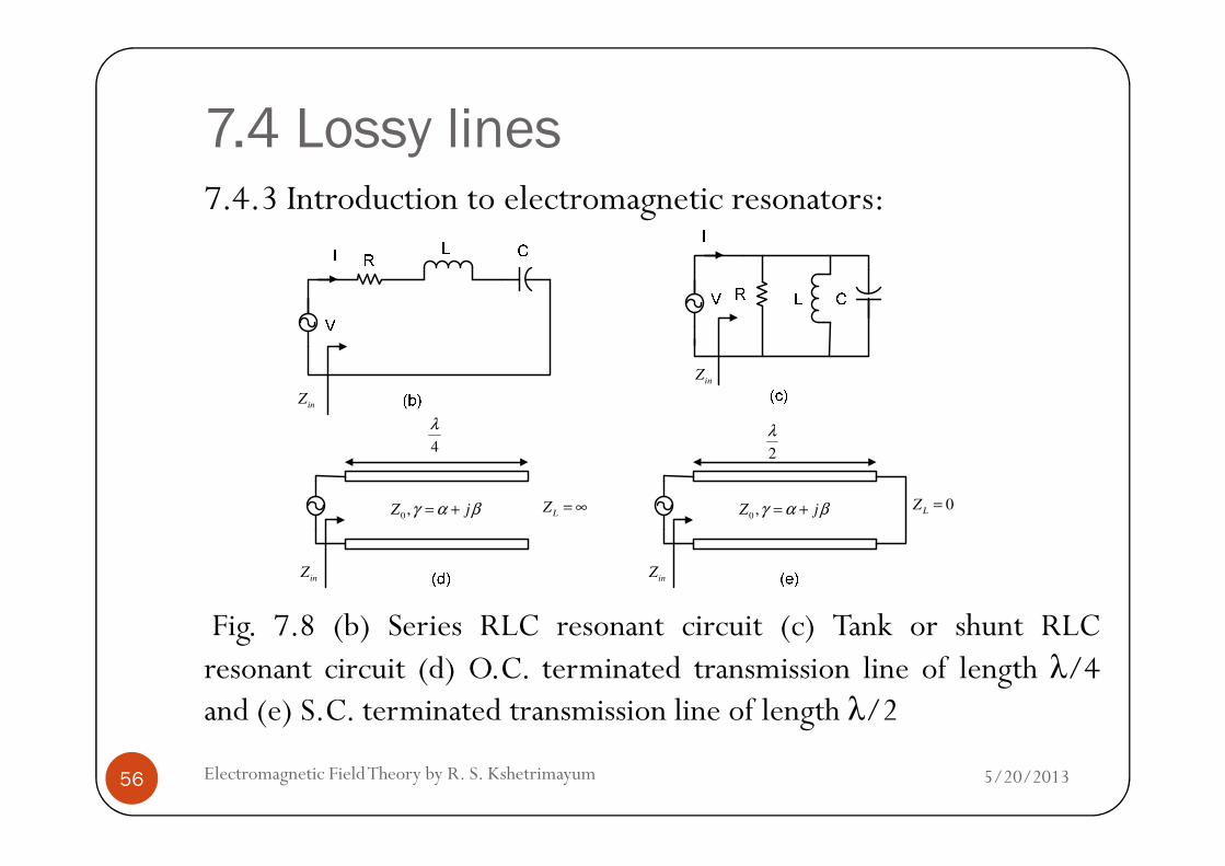
7.4 Lossy lines7.4.3 Introduction to electromagnetic resonators:

λ

inZ

inZ

λ


2

λ

0,Z jγ α β= + 0

LZ =

inZ

0,Z jγ α β= + L

Z = ∞

inZ

4

Fig. 7.8 (b) Series RLC resonant circuit (c) Tank or shunt RLCresonant circuit (d) O.C. terminated transmission line of length λ/4and (e) S.C. terminated transmission line of length λ/2

7.4 Lossy lines Microwave/electromagnetic resonators are used in many applications: filters,

oscillators,

frequency meters,


frequency meters,

tuned amplifiers, etc.

Its operations are very similar to the series and

parallel RLC resonant circuits

7.4 Lossy lines

We will review the series and

parallel RLC ciruits and

discuss the implementation of the microwave resonators using distributive elements such as microstrip line,


microstrip line,

rectangular and

circular waveguides, etc.

Series RLC resonant circuits

Consider the series RLC resonator

The input impedance Zin is given by1

inZ R j Lj C

ww

= + +

7.4 Lossy lines The average complex power delivered to the resonator is

The average power dissipated by the resistor is



21

2lossP I R=

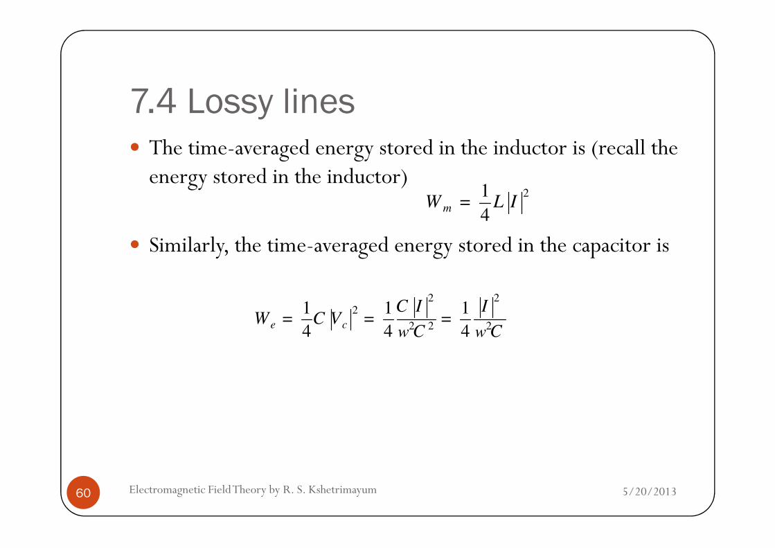
7.4 Lossy lines The time-averaged energy stored in the inductor is (recall the energy stored in the inductor)

Similarly, the time-averaged energy stored in the capacitor is

21

4mW L I=


2 22

2 2 2

1 1 1

4 4 4e c

C I IW C V

C Cw w= = =

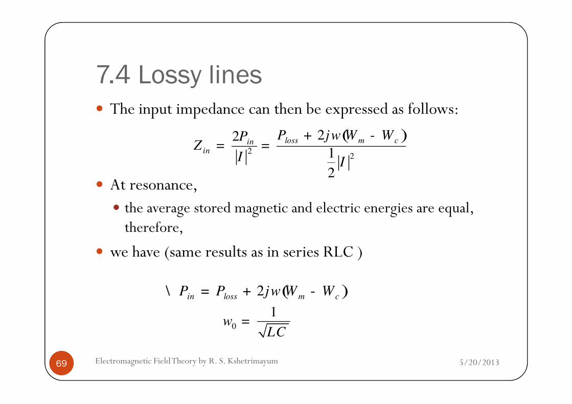
7.4 Lossy lines The input impedance can then be expressed as follows:

At resonance,

( )2 2

2 m elossinin

P j W WPZ

R R

w+ -= =

( )2in m elossP P j W Ww\ = + -


At resonance, the average stored magnetic and electric energies are equal,

therefore, we have

m eW W=21

2

lossin

PZ R

I

= =

7.4 Lossy lines Hence, the resonance frequency is defined as

The quality factor is defined as the product of the angular frequency and


the angular frequency and

the ratio of the average energy stored to

energy loss per second

7.4 Lossy lines Q is a measure of loss of a resonant circuit,

lower loss implies higher Q and

high Q implies narrower bandwidth

As R increases, power loss increases and


power loss increases and

quality factor decreases

Let us see what the approximate Zin near resonance

The input impedance can be rewritten in the following form:

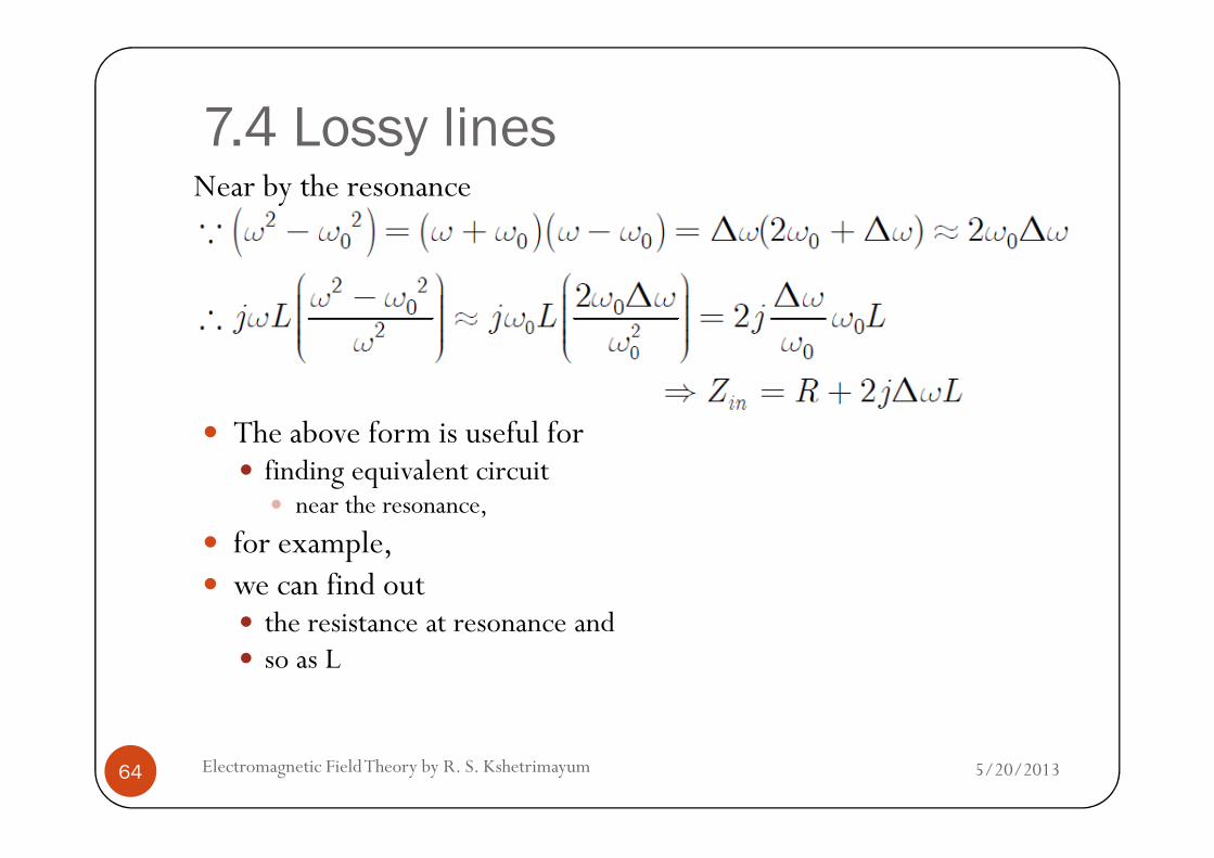
7.4 Lossy lines

The above form is useful for

Near by the resonance


The above form is useful for finding equivalent circuit

near the resonance,

for example, we can find out

the resistance at resonance and so as L

7.4 Lossy lines Half power fractional bandwidth

When the real power delivered to the circuit is half that of the resonance, occurs when

2inZ R=


7.4 Lossy linesShunt RLC Resonant Circuits

Now let us turn our attention to the parallel RLC resonator

The input impedance is equal to


7.4 Lossy lines The average complex power delivered to the resonator is


*1

2inP V I=

*

*

1

2 in

VV

Z=


21

2loss

VP

R=

7.4 Lossy lines The time-averaged energy stored in the inductor is (recall the energy stored in the inductor)


2 22

2 2 2

1 1 1

4 2 2m L

V VW L I L

L Lw w= = =



21

4cW C V=

7.4 Lossy lines The input impedance can then be expressed as follows:

At resonance, the average stored magnetic and electric energies are equal,

( )2

2

22

1

2

loss m cinin

P j W WPZ

I I

w+ -= =


the average stored magnetic and electric energies are equal, therefore,

we have (same results as in series RLC )

( )2in loss m cP P j W Ww\ = + -

0

1

LCw =

7.4 Lossy lines The quality factor, however, is different

Contrary to series RLC,


Contrary to series RLC, the Q of the parallel RLC increases

as R increases

7.4 Lossy lines Similar to series RLC,

we can derive an approximate expression for parallel RLC near resonance


7.4 Lossy lines As in the series case,

the half-power bandwidth is given by2

2

2in

RZ =


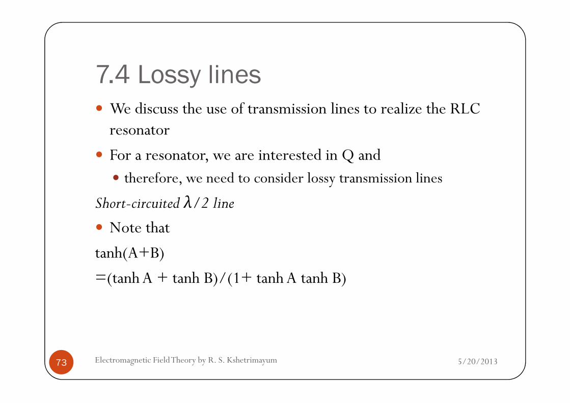
7.4 Lossy lines We discuss the use of transmission lines to realize the RLC resonator

For a resonator, we are interested in Q and therefore, we need to consider lossy transmission lines

Short-circuited λ/2 line


Short-circuited λ/2 line

Note that

tanh(A+B)

=(tanhA + tanh B)/(1+ tanhA tanh B)

7.4 Lossy lines

Consider the transmission line equation

tan( )[ ] / ( )

[ ] /x

e e j

e e

jx jx

jx jx====

−−−−

++++

−−−−

−−−−

2

2

tanh( )[ ] /

[ ] /x

e e

e e

x x

x x====

−−−−

++++

−−−−

−−−−

2

2


For a short-circuited line

7.4 Lossy lines Our goal here is to

compare the above equation

with input impedance of Series or

shunt RLC resonant circuit near resonance


so that we can find out the corresponding R, L and C

For a length l=λ/2 of the transmission line, assuming a TEM line so that

7.4 Lossy lines

For low-loss transmission lines, αl is small, hence

ββββ ωωωω µεµεµεµε ωωωω==== ==== / vp l vp o==== ====λλλλ ππππ ωωωω/ /2

ββββωωωω ωωωω

ππππωωωω

ll

v

l

v

l

vp

o

p p o

==== ==== ++++ ==== ++++∆ω∆ω∆ω∆ω ∆ωπ∆ωπ∆ωπ∆ωπ


For low-loss transmission lines, αl is small, hence

tan tan( ) tan( )ββββ ππππωωωω ωωωω ωωωω

lo o o

==== ++++ ==== ≈≈≈≈∆ωπ∆ωπ∆ωπ∆ωπ ∆ωπ∆ωπ∆ωπ∆ωπ ∆ωπ∆ωπ∆ωπ∆ωπ

7.4 Lossy lines Note that the loss is usually very small and

therefore, the input impedance can be rewritten as:


7.4 Lossy lines This equation can be compared favorably

with the input impedance of a series RLC resonant circuit near the resonance

It behaves like a series RLC resonator with


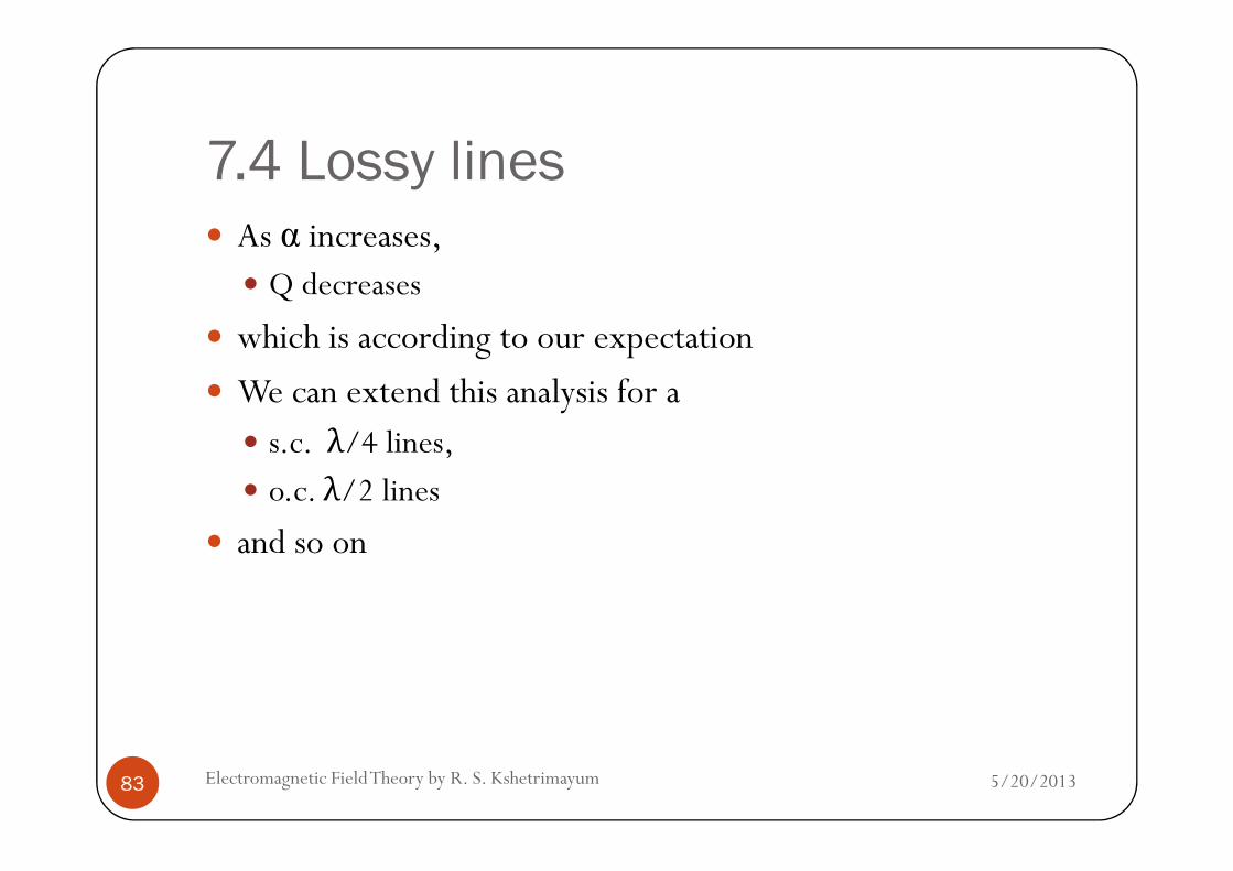
7.4 Lossy lines As α increases,

Q decreases

which is according to our expectation

Open-Circuited λ/4 Line

For a lossy line of length l


For a lossy line of length l

with propagation constant γ and

characteristic impedance Z0,

we can find the input impedance for a load of ZL as follows:

7.4 Lossy lines For o.c.,

For


l vp o==== ====λλλλ ππππ ωωωω/ / ( )4 2

ββββωωωω ωωωω ππππ

ωωωωl

l

v

l

v

l

vp

o

p p o

==== ==== ++++ ==== ++++2 2 2 2 2

∆ω∆ω∆ω∆ω ∆ωπ∆ωπ∆ωπ∆ωπ

7.4 Lossy lines

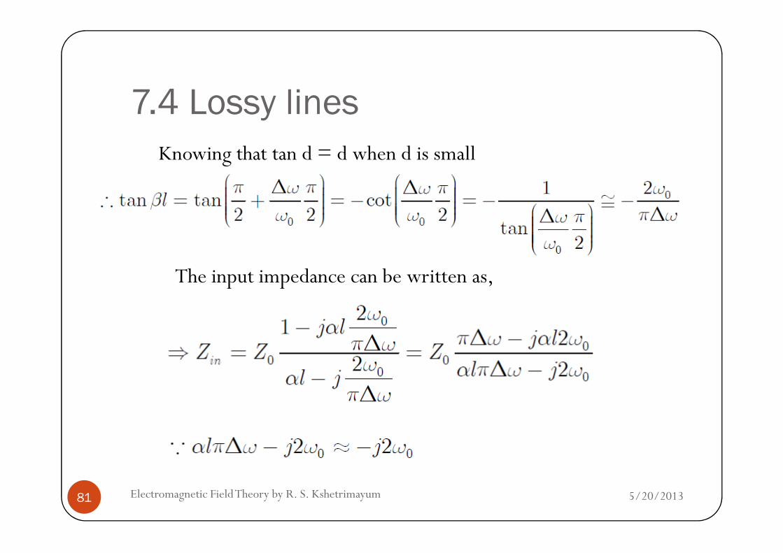
Knowing that tan d = d when d is small

The input impedance can be written as,


The input impedance can be written as,

7.4 Lossy lines

This equation can be compared favorably with the input impedance of a series RLC resonant circuit near the resonance


the resonance

It behaves like a series RLC resonator with

7.4 Lossy lines As α increases,

Q decreases

which is according to our expectation

We can extend this analysis for a s.c. λ/4 lines,


s.c. λ/4 lines,

o.c. λ/2 lines

and so on

7.5 Smith chart7.5.1 Impedance Smith chart

Smith chart is basically a graphical representation of

transmission line impedance transformation formula:


L 0

in 0

0 L

Z jZ tan( )Z Z

Z jZ tan( )

+ β=

+ β

l

l

7.5 Smith chart If we represent this in x-y coordinates with

x as real part and y as imaginary part of and

then it becomes a semi-infinite plane, not practical

We know that the

LZinZ


We know that the modulus of reflection coefficient (|Γ|) is always less than or equal to 1

And there is one to one correspondence between Γ andinZ

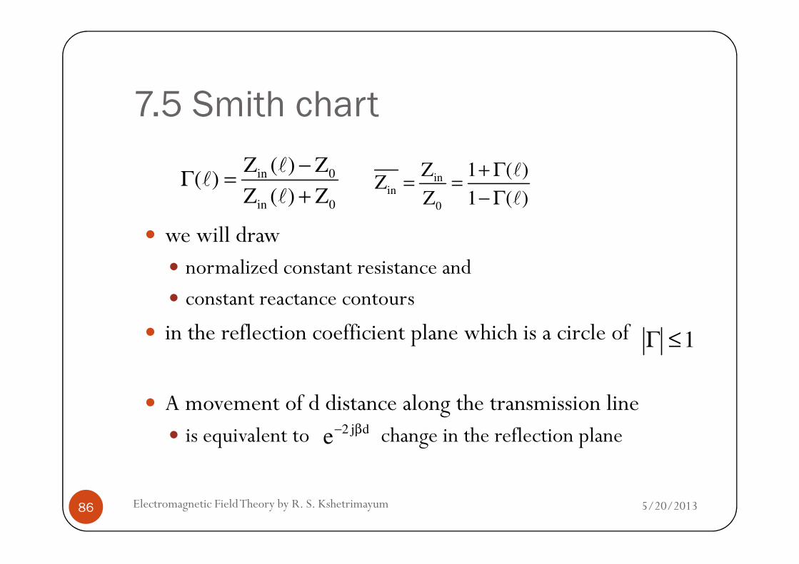
7.5 Smith chart

we will draw normalized constant resistance and

in 0

in 0

Z ( ) Z( )

Z ( ) Z

−Γ =

+

ll

l

inin

0

Z 1 ( )Z

Z 1 ( )

+ Γ= =

− Γ

l

l


constant reactance contours

in the reflection coefficient plane which is a circle of

A movement of d distance along the transmission line is equivalent to change in the reflection plane

1Γ ≤

2 j de− β

7.5 Smith chart Distance in movement in terms of wavelength is given in the circumference of the circle

It could be either towards load (WTL) or

source (WTG)


source (WTG)

At first glance, Smith chart looks intimidating with so many contours of

constant resistance and

reactance

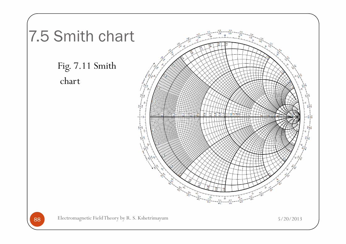
7.5 Smith chart

Fig. 7.11 Smith

chart


7.5 Smith chart Smith chart as a polar plot of Γ

(o.c. open circuit and

s.c. short circuit)

It can be simply


Γ

θ

j 0 0e , 180 180θΓ = Γ − ≤ θ ≤

It can be simply interpreted as a polar plot of

7.5 Smith chart The real utility of Smith chart lies

in the fact that we can read the corresponding normalized impedance value of Γ

from the constant reactance and resistance contours


in r iin in in

0 r i

Z 1 j1Z R jX

Z 1 1 j

+ Γ + Γ+ Γ= = + = =

− Γ − Γ − Γ

7.5 Smith chart constant resistance circles

constant reactance circles

( )2 2

2inr i

inin

R 1

R 1 R 1

Γ − + Γ =

+ +


( )22

2 111

=

−Γ+−Γ

inin

irXX

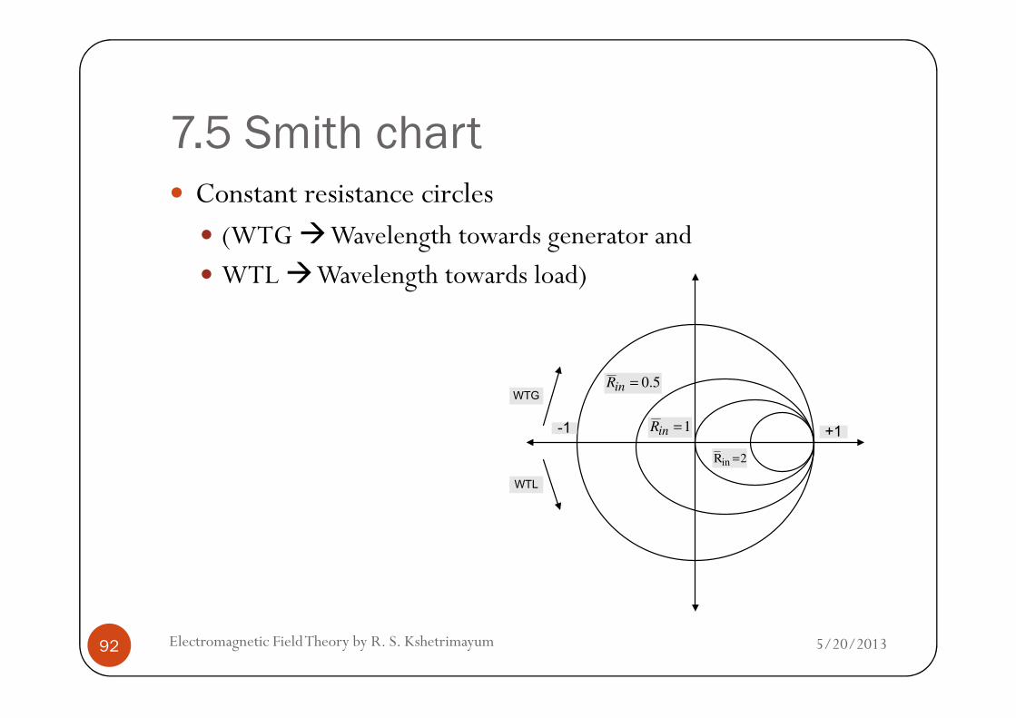
7.5 Smith chart Constant resistance circles

(WTG Wavelength towards generator and

WTL Wavelength towards load)


2Rin =

1=inR

5.0=inR

+1-1

WTG

WTL

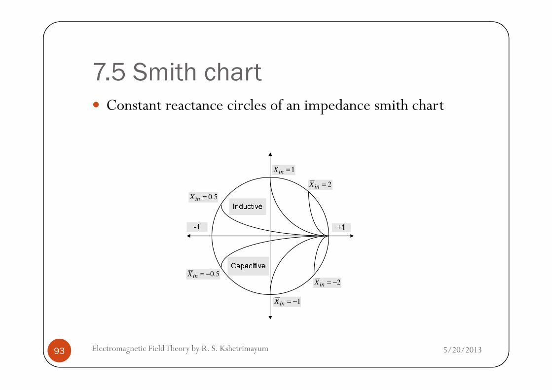
7.5 Smith chart Constant reactance circles of an impedance smith chart

2=inX

1=inX

5.0=X


2−=inX

1−=inX

5.0=inX

5.0−=inX

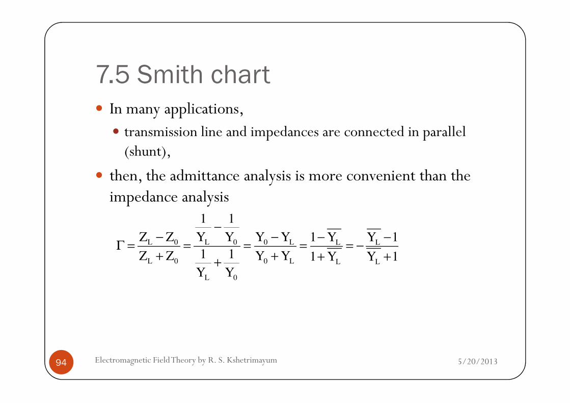
7.5 Smith chart In many applications,

transmission line and impedances are connected in parallel (shunt),

then, the admittance analysis is more convenient than the impedance analysis


impedance analysis

L 0 L 0 0 L L L

L 0 0 L L L

L 0

1 1

Z Z Y Y Y Y 1 Y Y 1

1 1Z Z Y Y 1 Y Y 1

Y Y

−− − − −

Γ = = = = = −+ + + ++

7.5 Smith chart Rules for conversion of impedance (say ZL at N) to admittance (say YL at N )

Γ


7.5 Smith chart The admittance smith chart is therefore obtained by

rotating the impedance Smith chart by π and

replacing r by g and x by b

Since it is just a matter of rotation, there is no need to have separate Smith charts for impedance


there is no need to have separate Smith charts for impedance and admittance

Although r and x can be interchanged with g and b respectively and

a point (r,x) and (g,b) will have the same spatial location on the Smith chart for r=g and x=b,

7.5 Smith chart But, the physical interpretation corresponding to the two will not be identical

Upper half of the impedance Smith chart with +jx represent inductive loads

whereas +jb represents


whereas +jb represents capacitive load on the admittance Smith chart

Point B on impedance Smith chart represents s.c.

whereas point B on admittance Smith chart represent o.c.

7.5 Smith chart Interchange on location of o.c./s.c. and

location of VSWR on an impedance Smith chart

Inductive/Capacitive


AB CD

Capacitive/Inductive

7.5 Smith chart Point A on impedance Smith chart which represents o.c.

whereas point A on admittance Smith chart which represents s.c.

Note that the distance between o.c. and s.c. is λ/4


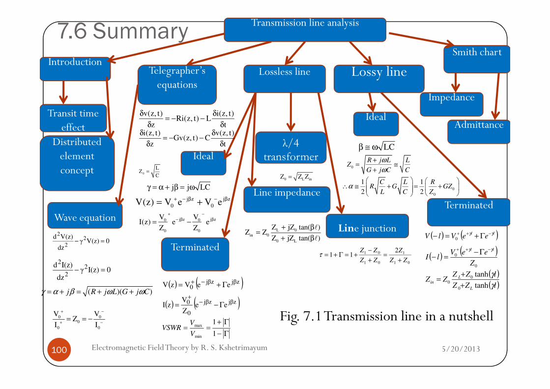
7.6 Summary Transmission line analysis

Introduction

Distributed element concept

Lossless line

Transit time effect

Telegrapher’s equations

λ/4 transformer

Line impedance

Ideal

Lossy lineSmith chart

Ideal

Impedance

Admittancev(z, t) i(z, t)

Ri(z, t) Lz t

δ δ= − −

δ δi(z, t) v(z, t)

Gv(z, t) Cz t

δ δ= − −

δ δ

j j LCγ = α + β = ω

0

LZ

C=

0 L inZ Z Z=

0

0

1 1

2 2

C L RR G GZ

L C Zα

∴ ≅ + = +

LCβ ≅ ω

0

R j L LZ

G j C C

ω

ω

+= ≅

+


Line junctionWave equation

Fig. 7.1 Transmission line in a nutshell

Line impedance

Terminated

Terminated

0V(z)γdz

V(z)d 2

2

2

=−

0I(z)γdz

I(z)d 2

2

2

=−

( )( )j R j L G j Cγ α β ω ω= + = + +

0 00

0 0

V VZ

I I

+ −

+ −= = −

j z j z

0 0V(z) V e V e+ − β − β= +

j z j z0 0

0 0

V VI(z) e e

Z Z

+ −

− β β= −L 0

in 0

0 L

Z jZ tan( )Z Z

Z jZ tan( )

+ β=

+ β

l

l

01

1

01

01 211

ZZ

Z

ZZ

ZZ

+=

+

−+=Γ+=τ

( ) ( )zβjzβj0 eeVzV Γ+= −+

( ) ( )zβjzβj

0

0 eeZ

VzI Γ−= −

+

Γ−

Γ+==

1

1

min

max

V

VVSWR

02 2L C Z

( ) ( )lleeVlV

γγ −++ Γ+=− 0

( ) ( )0

0

Z

eeVlI

ll γγ −++ Γ−=−

( )( )lZZ

lZZZZ

L

Lin

γ

γ

tanh

tanh

0

00

+

+=

7 slides

Documents

electromagnetic fieldtheory

electromagnetic energy

introduction radiation

introduction size effect

frequency of current

ac signal

kshetrimayum2 line junction

ac current flowing