726 ieee journal of oceanic engineering, … ieee journal of oceanic engineering, vol. 26, no. 4,...

726 IEEE JOURNAL OF OCEANIC ENGINEERING, VOL. 26, NO. 4, OCTOBER 2001

Spectral-Feature Classification of OceanographicProcesses Using an Autonomous Underwater Vehicle

Yanwu Zhang, Member, IEEE, Arthur B. Baggeroer, Fellow, IEEE, and James G. Bellingham

Abstract—The paper develops and demonstrates a method ofclassifying oceanographic processes using an autonomous-under-water vehicle (AUV). First, we establish the “mingled-spectrumprinciple” which concisely relates observations from a movingplatform to the frequency-wavenumber spectrum of the surveyedprocess. This principle clearly reveals the role of the AUV speedin mingling time and space. An AUV can distinguish betweenoceanographic processes by jointly utilizing temporal and spatialinformation. A parametric tool for designing an AUV spectralclassifier is then developed based on the mingled-spectrum prin-ciple. An AUV’s controllable speed tunes the separability betweenthe mingled spectra of different processes. This property is thekey to optimizing the classifier’s performance. As a case study,AUV-based classification is applied to distinguish ocean convec-tion from internal waves. It is demonstrated that at a higher AUVspeed, convection’s distinct spatial feature is highlighted to theadvantage of classification. Finally, the AUV classifier is testedby the Labrador Sea Convection Experiment of February 1998.We installed an Acoustic Doppler Velocimeter in an AUV and itmeasured flow velocity in the Labrador Sea. Based on the verticalflow velocity, the AUV-based classifier captures convection’soccurrence. This finding is supported by other oceanographicobservations in the same experiment.

Index Terms—Autonomous-underwater vehicle (AUV), classifi-cation, oceanographic process, spectral feature.

I. INTRODUCTION

ONEof themostchallenging tasks inobservingandstudyingtheocean’s temporalandspatialvariability is to identify the

underlying ocean process. The paper develops and demonstratesa method of classifying ocean processes using observations froman autonomous-underwater vehicle (AUV) [1].

Eulerian and Lagrangian platforms are representative oftraditional oceanographic monitoring tools [2]. An Eulerianplatform is fixed in location, providing time series recordsof measured quantities. Moored current meters and conduc-tivity-temperature depth (CTD) sensors have become a routinein oceanographic monitoring. A Lagrangian platform, on theother hand, drifts with the current flow. By tracking Lagrangianplatforms acoustically (e.g., SOFAR drifters) or by satellite

Manuscript received September 30, 2000; revised July 1, 2001. This workwas supported in part by the Office of Naval Research (ONR) under GrantN00014-95-1-1316 and Grant N00014-97-1-0470, in part by the MIT Sea GrantCollege Program under Grant NA46RG0434, and in part by the Ford Professor-ship of Ocean Engineering.

Y. Zhang is with Aware Inc., Bedford, MA 01730, USA (e-mail:[email protected]).

A. B. Baggeroer is with the Department of Ocean Engineering and the De-partment of Electrical Engineering and Computer Science of the MassachusettsInstitute of Technology, Cambridge, MA 02139 USA.

J. G. Bellingham is with the Monterey Bay Aquarium Research Institute,Moss Landing, CA 95039 USA.

Digital Object Identifier S 0364-9059(01)09919-8

(e.g., the ARGOS system) for surface floats, we can obtain afirst-order description of the global ocean circulation [3], [4].

Classification imposes a higher level of requirement thanmonitoring. To optimize classification, both temporal andspatial features should be utilized. Eulerian and Lagrangianplatforms have inherent limitations in this respect. Eulerianmeasurement is confined to a fixed location. Although amooring may sense some information of the field’s spatialvariation via a horizontal advective current, this kind of sensingis uncontrolled and tends to be ambiguous. Deploying an arrayof moorings can add in spatial coverage, but high cost wouldoften deter dense spatial sampling. A Lagrangian platformdrifts with zero relative velocity against the ambient flow. Itdoes move, but its motion is no different from the advectingcurrent. As a drifter is bound to a tagged parcel of water, it hashardly any chance to catch sight of the real spatial variation ofthe field.

Since Eulerian or Lagrangian platforms have limitations inproviding temporal plus spatial features of ocean processes, weresort to moving platforms with the intent to overcome this de-ficiency. A towed platform is tied to a surface ship. This type ofplatform is typically confined to a depth of no more than a fewhundred meters [5]. A larger depth slows the tow speed, limitsmaneuverability, and increases the cost of the cable and winchsystem.

An AUV [1] is an unmanned, untethered moving platform.An Odyssey IIB AUV, as shown in Fig. 1, can dive to the fullocean depth in most places. Its speed range is from 0.25 to2.5 m/s (the lower limit is for maintaining the vehicle’s con-trollability). Once equipped with a classification capability, anAUV has the promise of autonomously searching for oceano-graphic processes of interest. An AUV is neither Eulerian norLagrangian, but cruises through the ocean at a controllable andflexible speed, collecting information in both time and space.AUV measurements thus mingle temporal and spatial variationsof the sampled field. We establish the mingled-spectrum prin-ciple in Section II.

According to the mingled-spectrum principle, an AUVcan distinguish between oceanographic processes by jointlyutilizing temporal and spatial information. Our goal is not toreconstruct the field [6]–[9] or its original spectrum [10], butto classify the fields by the difference between their respectivemingled spectra acquired by an AUV. Hence, we are to utilizethe mingling of time and space to the advantage of classifi-cation, rather than regarding the mingling as a contaminatingfactor [11]. In Section III, we develop a parametric tool fordesigning an AUV-based classifier. It is shown that an AUV’scontrollable speed tunes the separability between the mingled

0364-9059/01$10.00 © 2001 IEEE

Authorized licensed use limited to: Monterey Bay Aquarium Research Inc. Downloaded on July 21, 2009 at 14:37 from IEEE Xplore. Restrictions apply.

ZHANG et al.: SPECTRAL-FEATURE CLASSIFICATION OF OCEANOGRAPHIC PROCESSES 727

Fig. 1. An Odyssey IIB AUV being recovered after operations.

Fig. 2. A line AUV survey.

spectra of different processes. This property is the key to opti-mizing the classifier’s performance. In Section IV, we present atest case for AUV-based classification: ocean convection versusinternal waves. At last, the AUV-based classifier is tested bythe 1998 Labrador Sea Experiment data, as given in Section V.

II. MINGLED-SPECTRUM PRINCIPLE

A. Mingled Spectrum Recorded by a Moving Platform

An oceanographic process varies both in time and space. Weassume that a studied process is temporally stationary and spa-tially homogeneous. Then, the oceanographic field can be de-scribed by its frequency -wavenumber spectrum. When an AUV(or some other moving platform) carries out a survey in the field,it records a time series of some measured quantity, e.g., flow ve-locity. The time-series mixes temporal and spatial variations ofthe surveyed field. The corresponding spectrum therefore min-gles the spectral information of time and space, hence we call ita “mingled spectrum”.

An elementary survey mode is along a line, as illustrated inFig. 2. Consider a scalar process under survey. Denote itsvariation on the survey line as , where is time and islocation. Denote the time series recorded by the AUV as ,assuming no sensor error. At an AUV speed of , the autocor-relation function of is related to that of by

(1)

Under the assumptions of temporal stationarity and spatialhomogeneity, we apply the Wiener-Khinchine theorem [12].The power spectrum density (PSD) of , i.e., the mingledspectrum, is the Fourier transform of

(2)

where is temporal frequency.For the temporal-spatial process , its autocorrelation

function and its PSD are Fourier transformpairs (also by the Wiener–Khinchine theorem [12])

(3)

where is the temporal frequency, and is the spa-tial frequency. Note that is a one-dimensional wavenumber inthe direction of AUV’s line survey. Sign convention is in accor-dance with that of propagating waves [13].

Incorporating (3) into (2), we have

(4)

Hence, the mingled spectrum is the integration overof on a line defined by , as illustrated in



Fig. 3. Illustration of the mingled-spectrum principle. The blue line is theintegration line, which intercepts with �-axis at � = f . The integration lineslides from left to right to produce the mingled spectrum as a function of f . Ata higher AUV speed, the red line becomes the integration line.

Fig. 3. The integration line’s slope equals the reciprocal of AUVspeed . The integration line’s intercept on the -axis equals

. Equation thus con-cisely reveals the relationship between the “AUV-seen” min-gled spectrum and the original temporal-spatial spectrum

.It can be demonstrated [14] that: 1) platform speed ; or

2) a temporally frozen field; or 3). a nondispersive plane wave,are just several special cases under which the mingled-spectrumformula reduces to forms we are familiar with. Compared withthe Doppler shifted-spectrum method [15], the mingled-spec-trum principle provides advantages of applicability to isotropyor anisotropy, ease for inspection, and simplicity of computa-tion [14].

B. Utilization for AUV-Based Classification

Let us first look at two simple fictitious temporal-spatial fieldsfor the purpose of demonstration. Their – spectra are ex-pressed in (5) and (6), and displayed in the upper panel of Fig. 4.The – spectrum of field no. 2 is just a transpose of that of fieldno. 1. In both spectra, the range of frequency is from –1 to 1Hz, while the range of wavenumber is from –1 to 1 m .

(5)

(6)

where , , .The spectrum of the AUV-recorded time series in a line

survey is the mingled spectrum formulated in (4). The mingledspectrum, rather than the field’s original frequency wavenumberspectrum, is the information source for spectral classification,because time and space are already mixed in the AUV’s record.As revealed by (4) and Fig. 3, time-space mixing is tuned bythe AUV speed as the integration is constrained by a linewhose slope equals .

Fig. 4. Derivation of mingled spectra from the two fictitious �–� spectra. Theslanted line is the integration line, which slides from left to right to produceS (f).

For the above two fictitious fields, their mingled spectra ascomputed by (4) is illustrated in the lower panel of Fig. 4. Ata series of vehicle speeds, the two mingled spectra are shownin Fig. 5. The observation is: the two mingled spectra may ap-pear more alike or more distinct depending on the AUV’s cruisespeed. Due to the “transpose” relation between the two hypoth-esized – spectra, their mingled spectra are identical when theAUV cruises at a speed of 1 m/s (the third panel of Fig. 5). Thiswould obviously prohibit classification. At other speeds of 0.5m/s (the second panel) and 2 m/s (the fourth panel), however,the two processes are classifiable as their mingled spectra showdifference. A quantitative metric for separability will be givenin Section III.

It should be noted that our goal is not trying to reconstructthe field [6]–[9] or its original spectrum [10], but to classify thefields by the difference between their respective mingled spectraacquired by an AUV. From this standpoint, we are to utilize themingling of time and space to the advantage of classification,rather than regarding the mingling as a contaminating factor[11].

III. AUV-BASED SPECTRAL CLASSIFICATION

A. Classifier Architecture

The AUV-based classifier’s architecture is illustrated inFig. 6. The scope of our study is confined to two classes, de-noted by and ( stands for “Hypothesis”), respectively.AUV’s measurement is the input to the classifier.mingles temporal and spatial variations of the field, and its PSD

is a mingled spectrum. It is related to the field’s tem-poral-spatial PSD by the mingled-spectrum formula(4). From AUV’s measurement , we obtain an estimate ofits PSD, . Hereafter, we denote the true PSD asand its estimate as (for class 1 and 2, footnotes “1” and“2” are added for distinction). Classification [16], [17] relies onthe “distance” (i.e., the spectral separability) between the two



Fig. 5. Mingled spectra of the two fictitious fields.

Fig. 6. Diagram of the AUV-based spectral classifier.

mingled spectra and . The AUV speed tunesthis distance.

We use the Fourier method of periodogram [18], [19] forspectrum estimation, so is given at a series of discretefrequencies. Thus, the PSD estimate is expressed as a columnvector , , where is the total numberof frequency points. In consideration of instrument noise, thereexists an upper bound of usable frequency range for classifica-tion, as will be detailed in Section IV-C.

A scalar feature is then extracted from vector through alinear transformation

(7)

where is the feature projection vector.We adopt the Fisher’s separability metric [17] to measure the

“distance” between spectra in the two classes. Under this metric,

it can be proven [17] that all separability information is pre-served despite the -dimension one-dimension projection.

Finally, the scalar feature passes a threshold comparator tomake the classification decision ( or ). The threshold isdetermined by minimizing the total cost or probability of error(the Bayesian criterion), or by satisfying some prescribed falsealarm probability (the Neyman–Pearson criterion) [16].

B. Feature Projection Vector

The feature projection vector is clearly the key to the clas-sifier. is formulated as follows [17]:

(8)

where

(9)

is the mean spectrum in each class and

(10)

is the within-class scatter matrix that depicts the scatter ofaround its mean spectrum in each class. is the a priori prob-ability of class , and is the covariance matrix in class

(11)



Fig. 7. Mechanism of feature projection when the two-dimensional � isdiagonal with � (1) > � (2), i = 1; 2.

To help explain ’s mechanism, let us consider a verysimple case. Suppose vector has only two components, asshown in Fig. 7. If were diagonal with equal elements

, would be a scaled identity matrixand would simply coincide with the vector of differencebetween the mean vectors: . When is stilldiagonal but with unequal elements: e.g., asshown in Fig. 7, will no longer be a scaled identity matrixbut will play a role in the formation of . As Fig. 7 illustrates,the role of is to rotate away from the -axis andtoward the -axis. This rotating represents a penalty onthe -axis projection because the uncertainty of islarger than that of . The separability between the twoclusters of feature is maximized using the rotated .

To compute , we need to know mean spectra and, as well as covariance matrices and of the

two processes of interest. We choose frequency points with aninterval of the finite data window’s bandwidth. So the PSD es-timates at those frequencies are uncorrelated [19]. Covariancematrix is consequently diagonal, where the diagonal ele-ments are spectrum variance at the chosen frequen-cies.

For each oceanographic process, we use a model to obtainits temporal-spatial PSD (examples will be given inSection IV). The mingled spectrum is then derived from

by (4). We regard the resultant (with the ad-ditional consideration of the finite data window effect) as themean spectrum ( or 2).

The PSD estimate’s variance originates fromtwo sources: periodogram’s inherent uncertainty and modelparameter uncertainty. The periodogram method [18], [19]dictates that the PSD estimate’s variance is proportional to

, where the coefficient is determined by the set-tings in time-domain segmentation and frequency-domainsmoothing. Model-parameter uncertainty describes possiblemismatch between the model and the real data. To build thespectrum template in each class, we assign a set of parametersto the corresponding model. Those parameters are selected

Fig. 8. Illustration of the convection model box. Only the top surface issubjected to a heat flux. The dimension is 200� 200� 35 with a grid size of10 m.

TABLE IMIT CONVECTION MODEL PARAMETERS

based on our understanding of the process and available priorinformation. Parameters of the real data, however, may havesome discrepancy from the model’s. This mismatch is referredto as parameter uncertainty. In formulating , wehave taken into account both uncertainty sources. Due to spacelimit, the formula and its derivation are omitted. By includingmodel parameter uncertainty in the design, the classifier ismade robust to model mismatch.

IV. TEST CASE: OCEAN CONVECTION VERSUS INTERNAL

WAVES

We introduce two oceanographic processes for demonstratingAUV-based classification. They are ocean convection and in-ternal waves. Vertical flow velocity is a key signature of bothprocesses [20], [21]. Thus we select it as the quantity(shown in Fig. 2) for classification. Prospects of introducingmore quantities (e.g., temperature) to improve classification willbe discussed in Section VI.

A. Ocean Convection

Convection is the transfer of heat by mass motion of fluid[22]. It happens when the density distribution becomes unstable[3]. Open ocean convection takes place at only a few locationsaround the world, namely, the Labrador Sea [23], the GreenlandSea [20], Mediterranean [21], and around the Antarctica [24].



Fig. 9. Horizontal and vertical cross sections of convective vertical flow velocity w at time 7.4 h. Unit of horizontal bars is m/s.

At those locations, strong winter cooling of the surface watercauses it to become denser than the water beneath. The cooledsurface water sinks and mixes with deeper water which entersthe global ocean circulation. This process releases heat fromthe overturned water to the atmosphere and thus maintains amoderate winter climate on the land. Hence, ocean convectionis an important mechanism for global heat transfer [25].

Prof. John Marshall and his group at the MIT Department ofEarth, Atmospheric, and Planetary Sciences have constructed anumerical model of open ocean convection [26], [27]. We usethis model to find the temporal-spatial spectrum of convectivevertical velocity.

The model is configured as a box as shown in Fig. 8.Water is cooled at the top surface. There is no normal heatflux at the bottom or the four side walls. The parameters ofsurface heat flux and mixed-layer depth are set by using themeteorological and hydrographic data acquired during AUVMission B9 804 107 in the 1998 Labrador Sea Experimentthat will be presented in Section V. It is noted that owing toconsideration of model parameter uncertainty, the classifieraims to be robust to significant discrepancies between model

parameters and real data parameters. Main model parametersare listed in Table I. Note that the model’s dimensional scaleis on the order of 1 km.

At 26 520 s (about 7.4 h) after surface cooling starts, themodel output of vertical flow velocity is shown in Fig. 9. Theupper panel displays the horizontal cross section at the 250-mdepth, the same depth of AUV Mission B9 804 107. The lowerpanel displays the vertical crosssection at m. Con-vective cells with periodicity of 200 m–250 m are observable inboth panels.

Based on the model output for two hours (from 5.4 to 7.4 hafter the onset of surface cooling), we compute the temporal-spatial PSD of convective vertical velocity , as shown in theupper panel of Fig. 10 (while the mingled-spectrum principledoes not rely on isotropy, we consider the convection field to beisotropic because of the isotropic surface cooling in the model.Based on symmetry properties, the whole – spectrum is con-structed using the first quadrant). Temporally, the vertical-ve-locity field varies little during the two-hour evolution as con-vection approaches a stationary state. The observed basebandspectrum on the -axis is mostly due to the two-hour window



Fig. 10. Temporal-spatial PSD of vertical velocity of convection (upper) and internal waves (lower, with an extended plateau). Unit of vertical bars is10 log ((m/s) =(Hz � m )).

(the Fourier transform of a boxcar window is a sinc function).on the -axis, however, there is a peak at about 0.005 m be-cause convective cells have a spatial periodicity of about 200 m.We can utilize the AUV’s speed to highlight this feature of con-vection for classification against internal waves.

B. Internal Waves

Internal waves occur in the ocean’s interior. It is the water’sresponse to a disturbance to its equilibrium of hydrostaticallystable density stratification, via the gravitational restoring force[28]. Unlike convection which occurs in a vertically unstable ormixed water column, internal waves are found in stably strati-fied water. Stable stratification is depicted by the buoyancy fre-quency (also called the Brunt-Vaisala frequency) [29] that is de-termined by the density profile.

Internal waves play an important role in mass and momentumtransfer in the ocean [11]. Their dynamics is essential for un-derstanding the ocean circulation and temperature and salinitystructures [11]. In another aspect, sound-speed fluctuations in-duced by internal waves are a dominant source of the high-fre-quency variability of acoustic wave fields in the ocean [30].

Based on the Garrett-Munk model [11], [15], [31], [32],we derive the temporal-spatial PSD of internal-wave verticalvelocity. The spectrum is confined within a frequency range

Fig. 11. Derivation of mingled spectra from temporal-spatial spectra ofconvection and internal wave vertical velocities.

of Coriolis frequency ( Hz wherecycle/day is the angular velocity of Earth’s rotation

and N is the latitude of the 1998 Labrador Sea Exper-iment site) and buoyancy frequency (taken as Hz,



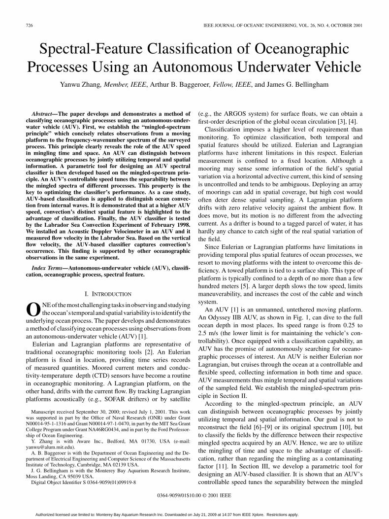
Fig. 12. Mingled spectra of vertical velocities of convection and internal waves. Abscissa is frequency in hertz; the unit of ordinate is 10 log ((m/s) =Hz).

equivalent to nearly three cycles per hour [32]). In the ocean,however, processes of frequencies higher than the buoyancyfrequency do exist [11], like turbulence [4]. We therefore needto consider higher frequency processes along with internalwaves. We add a spectrum plateau above the buoyancy fre-quency to account for higher-frequency processes. Based on aPSD plot of ocean wave kinetic energy, we calculate the ratioPower above buoyancy frequency Power of internal waves .

This ratio is then used to set the plateau’s height. Althougha plateau is not an accurate description of the spectrum, wedeem it sufficing to serve the purpose of this case study sincethe forthcoming computation of mingled spectrum is in anintegration sense. From the perspective of classification, thespectrum extension will prevent a classifier from unduly takingadvantage of a vanishing part of a spectrum (referred to as“singular detection” [16], [33] in detection theories).

With this plateau extension above the buoyancy frequency,the temporal-spatial PSD of internal wave vertical velocity isshown in the lower panel of Fig. 10. Note that for the sake oftesting the classifier, we have scaled internal wave vertical ve-locity’s amplitude such that its power equals that of convectivevertical velocity. On the -axis, most power lies at very lowwavenumber, showing no peak away from . In contrast,the temporal-spatial PSD of convective vertical velocity has aspectral peak at about m due to convective cells’periodicity, as shown in the upper panel of Fig. 10. This distinc-tion is what a cruising AUV can take advantage of for classifi-cation, as will be seen in the following.

C. Mingled PSDs at a Series of AUV Speeds

Having obtained of convective and internal wavevertical velocities, let us derive the AUV-seen by the

mingled-spectrum principle, as illustrated in Fig. 11. Convec-tion’s spatial peak on the -axis is projected onto the -axis ofthe corresponding mingled spectrum. At a higher AUV speed,the spectral peak on the -axis is pulled farther away from

. For internal waves, however, the picture is different. Since in-ternal waves’ power is concentrated at baseband on the -axisand the -axis, the corresponding mingled spectrum also lies atbaseband on the -axis. A higher AUV speed will not changethis basic spectral shape. Based on this inspection even beforeconducting computations, we project that the distinction be-tween the two spectra will enlarge with AUV speed.

We apply (4) at a series of AUV speeds m/s, 0.25m/s, 0.1 m/s, and 0.05 m/s. The resultant mingled spectra ofconvective and internal wave vertical velocities are comparedin Fig. 12. Data window effect has been included in the calcula-tions. The window length is set to 1400 s to coincide with that ofthe AUV’s Labrador Sea experimental data which will be pre-sented in Section V. The results in Fig. 12 are consistent withthe predictions inspected from Fig. 11.

In consideration of instrument noise, there exists an upperbound of usable frequency range for classification. We requirethat across this valid frequency range, mingled spectra of bothprocesses maintain a signal-to-noise-ratio (SNR) of 20 dB overthe instrument noise floor of the acoustic Doppler velocimeter(ADV) under normal operation conditions (an AUV-borne ADVacquired the flow velocity data in the Labrador Sea Experiment,as will be presented in Section V). At a lower AUV speed, spec-trum levels drop more steeply toward high frequency, thus thevalid frequency range shrinks as the vehicle speed decreases.The upper bound of valid frequency range is 0.009, 0.006, 0.004,and 0.003 Hz at AUV speed m/s, 0.25 m/s, 0.1 m/s, and0.05 m/s, respectively. Taking those ranges into account, we see



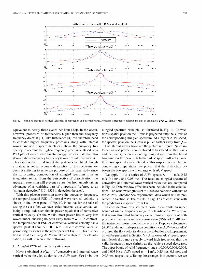
Fig. 13. Histogram of scalar feature z in class 1 (internal waves, upper panel) and class 2 (convection, lower panel) at AUV speed 0.25 m/s.

that the mingled-spectrum pairs are much more distinguishableat higher AUV speeds.

D. Classifier Test Results of Model Based Simulations

For simulating a line AUV survey in the convection field, theAUV-recorded time series is directly drawn from the convectionmodel at depth 250 m. An ensemble of 200 AUV survey linesare used for every classifier test at each prescribed AUV speed.To add randomness to different test runs, the starting time andlocation are randomly picked (within range).

In the internal wave field, we simulate a line AUV surveytime series by passing white noise through a first-order (at AUVspeed m/s) or second-order (at AUV speed m/s)autoregressive (AR) model [34]. This method is suggestedby the shape of the mingled spectrum: e.g., at AUV speed

m/s, the mingled spectrum approximately follows apower law of at low frequency and at high frequency.Parameters of an AR model are selected such that its outputspectrum best matches the mingled spectrum. Two hundredAUV survey lines in the internal wave field are randomlygenerated in every classifier test.

Now we test the classifier. For each time series of AUV data,its PSD estimate is converted to a scalar feature by the trans-formation vector following (7). For each test, 200 lines ofAUV data in the convection field and another 200 lines in theinternal wave field are used. Classifier performance is evaluatedby the statistics of the resultant ensemble of .

Corresponding to Fig. 12, we test the classifier at a series ofAUV speeds m/s, 0.25 m/s, 0.1 m/s, and 0.05 m/s. At

m/s, histograms of scalar feature in the two classesare shown in Fig. 13. In each panel, there are 200 values(binned). Histogram of shows its statistical distribution. Let usdefine the false alarm probability as that of declaring con-vection when internal wave is true; the detection probabilityas that of declaring convection when convection is indeed true.The classifier’s – relationship is depicted by the receiveroperating characteristic (ROC [16]), as shown in Fig. 14. Notethat the ROC curve is determined solely by the probability dis-tribution functions of , not by the detection threshold.

At lower AUV speeds 0.1 m/s and 0.05 m/s, histogramsof scalar feature in the two classes severely overlap (plotsomitted). The corresponding ROC curves are shown in Fig. 14.We know that a lower ROC curve implies a lower classifier per-formance, the worst being the diagonal line which is equivalentto flipping a coin. Thus, at lower AUV speeds, classificationappears to be more difficult. This is an expectable outcome bycomparing the mingled spectrum pairs in Fig. 12 (also keepingin mind valid frequency ranges as given in Section IV-C). At alow vehicle speed, convection’s spatial variation cannot be wellsensed by the AUV, so the recorded time series is basically stilllow-pass, similar to an internal wave measurement.

At a higher AUV speed, convection’s spatial peak onthe -axis is apparently projected onto the -axis of thecorresponding mingled spectrum, as displayed by Fig. 11.Thus convection’s spatial feature is brought to light in theAUV-recorded time series. Due to the properties of internalwave’s frequency -wavenumber spectrum, its mingled spectrumlies at baseband on the -axis. A higher AUV speed does not



Fig. 14. Classifier’s performance (P versus P ) at a series of AUV speeds.

change this basic spectral shape. A higher AUV speed thuspulls the peak of convection’s mingled spectrum farther awayfrom the base-frequency band where the internal wave staysdespite the heightened vehicle speed. This highlighted differ-ence improves the classifier’s performance. At AUV speed of1 m/s, the two clusters of scalar feature do not overlap, as willbe shown in Fig. 22. This indicates a even better classificationperformance than at AUV speed 0.25 m/s.

We have also tested the classifier’s robustness by using inputdata that is mismatched with the model. For convection, we letthe heat flux and the mixed layer depth both increase by a factorof three. This implies a significant change of the environment.As a consequence, convection’s mingled spectrum gets closer tothat of internal waves, making classification more challenging.Since we have incorporated model parameter uncertainty (factorof three in this case study) into the feature projection vector

in Section III-B, the classifier is prepared to the above mis-match. The classifier’s performance (ROC curves omitted dueto space limit) shows only a slight degradation compared withthe matched case. It still holds true that a higher AUV speedbetter highlights convection’s spatial feature so as to improveclassification.

V. LABRADOR SEA EXPERIMENT

A. Background

The Labrador Sea lies between northern Canada and Green-land. It is one of the few locations in the world where open oceanconvection occurs [23], [35]. During the winter, the sea surfaceis subjected to intense heat flux to the atmosphere. The resultingbuoyancy loss causes the surface water to sink to large depths,initiating ocean convection.

During January/February 1998, researchers from the Mass-achusetts Institute of Technology, the Woods Hole Oceano-

Fig. 15. Ship track of R/V Knorr during the 1998 Labrador Sea experiment.The focal region marks the experiment site. (Courtesy of Dr. Knut Streitlien).

graphic Institution, and the University of Washington, made anexpedition to the Labrador Sea to study ocean convection. TheResearch Vessel (R/V) Knorr was employed in this experiment.The map of the Labrador Sea area as well as the ship track isshown in Fig. 15 (The cruise number was KN156). AUVs andother oceanographic platforms (e.g., Lagrangian floats) weredeployed in this experiment.

B. AUV-Borne Flow Velocity Measurement

We installed an ADV [36] in an Odyssey IIB AUV to measureflow velocity in the Labrador Sea. An ADV probe is illustratedin the left panel of Fig. 16. The acoustic beams of the transmitterand the three receivers intersect at a small sampling volume2 cm located away from the instrument base (16 cm distancefor Model ADVOcean we installed). Three-dimensional flowvelocity at this distant focal point is calculated based on theDoppler principle. An ADV’s spatial focus and low noise makeit suitable for experiments that require high-resolution and high-precision [37].

With careful considerations of various installation con-straints, we mounted the ADV at the AUV’s largest verticalcross-section, with its probe pointing 45 from the vehicle’shorizontal central plane, as shown in the right panels of Fig. 16.The ADV’s three receiver tips reach the brink of the vehicle’souter fairing but do not protrude beyond it. Inside the vehicle,the ADV probe is mounted with a horizontal plate and a 45slanted bracket. During installation, we use a laser pointer toensure alignment accuracy.

The AUV-borne ADV measures flow velocity relative to themoving vehicle. Hence, to obtain the Earth-referenced flow ve-locity, i.e., the true flow velocity, we must subtract the vehicle’sown velocity from the raw measurement. Another effect to re-



Fig. 16. Side view of an ADV probe (left), and cross-sectional view and side view of the ADV’s mounting on the vehicle (right). In the upper right panel, thebig circle represents the vehicle’s outer fairing. In the lower right panel, the lower half of the vehicle’s inner fairing is placed upside-down for ease of installation,while the outer fairing is removed.

Fig. 17. AUV behavior sequence in Mission B9 804 107.

move is the vehicle hull’s influence on the measurement. To as-certain this effect, we carried out a calibration experiment in theDavid Taylor model basin, utilizing its large tank cross sectionand precise speed control of the carriage.

The Earth-referenced vertical flow velocity is extractedthrough the following steps [38]. 1) Transform the velocitymeasurement from the ADV coordinate system to the AUVcoordinate system. 2) Compensate for the AUV hull’s influenceand subtract the velocity induced by the vehicle’s rotation.3) Recover the relative flow velocity in the Earth coordinatesystem using the vehicle’s heading, pitch, and roll measure-ments. 4) Subtract the vehicle’s own vertical velocity which isobtained by differentiating its depth sensor measurement. Thusthe Earth-referenced vertical flow velocity is obtained.

TABLE IIMEASUREMENT/ESTIMATION NOISE

* For AUV mission B9804017 on the 1998 Sea Experiment.

AUV Mission B9 804 107 took place at 4:46–7:00 on Feb-ruary 10, 1998 (GMT). The mission launch location was about

N, W, where the autonomous oceanographic sam-pling network (AOSN[39]) mooring was anchored. The AUVbehaviors in this mission are illustrated in Fig. 17. The vehiclefirst spiraled down to 426-m depth, then it spiraled up to 250-mdepth. At this depth plane, the vehicle made a “diamond” run,i.e., closed a four-leg loop with 90 turns, each leg lastingfor 720 s. After that, it spiraled up to 20-m depth, making anidentical “diamond” run. At the end, the vehicle ascended tothe sea surface. The vehicle’s speed in level legs was about1 m/s.

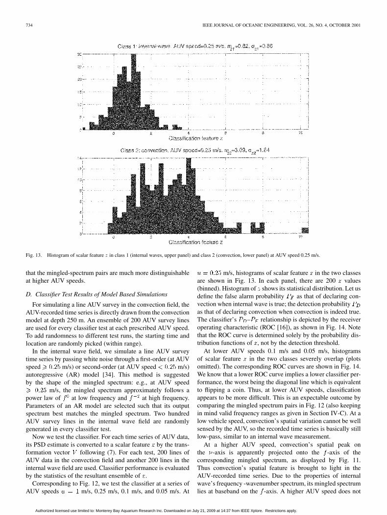
The Earth-referenced vertical flow velocity (denoted as) at the 250-m depth is extracted and shown in the first

panel of Fig. 18. The vehicle’s own vertical velocity (the secondpanel) has been removed for producing . It is noted thatthe 250-m depth is within a 350-m mixed layer (to be shown inSection V-C).



Fig. 18. The Earth-referenced vertical flow velocity w (the first panel) at the 250-m depth of AUV Mission B9 804 107. In the second panel is the AUV’sown vertical velocity. The AUV’s roll (the third panel) shows when the vehicle made 90 turns.

Fig. 19. Profiles of potential temperature, salinity, and potential density during AUV Mission B9 804 107.

The total noise in results from three sources ofmeasurement noise: i) ADV; ii) KVH heading/pitch/roll and ratesensor; iii) AUV’s depth sensor. The source errors propagate into

the final result by matrix transformations in convertingraw measurements to Earth-referenced flow velocity. Error



Fig. 20. PSD estimate of w at the 250-m depth of AUV Mission B9 804 107. Using five-point frequency-domain smoothing, the 1�� error band is shown.

sources and the total noise in (all after 50-s smoothing)are summarized in Table II [38].

C. Test of AUV-Based Classifier by Labrador Sea Data

Meteorological data were recorded by an improved meteo-rological (IMET) system [40] on board R/V Knorr. Prof. PeterGuest of the Naval Postgraduate School calculated the oceansurface heat flux based on the measurements. During AUVMission B9804107, the heat flux was about 300 W/m . Letus make comparisons with previous open ocean convectionexperiments. In the Greenland Sea Experiment [20] during thewinter of 1988/1989, the heat flux fluctuated between 100 and500 W/m , with an average value of about 250 W/m . Oceanconvection was observed during that experiment, using mooredacoustic Doppler current profilers (ADCPs). In an earlierLabrador Sea experiment [35] during the winter of 1994/1995,the average heat flux was about 300 W/m . Using a mooredADCP and profiling autonomous Lagrangian-circulation ex-plorer (PALACE) floats, ocean convection was observed. Thesea-surface heat flux value in our Labrador Sea Experimentis close to that of the two previous experiments. We thereforehave reason to expect ocean convections occurring.

Besides surface heat loss, a vertically mixed water columnis another key indicator of ocean convection. Across theLabrador Sea basin (about 600 km), a mixed water layer ofdepth 270 m–500 m was observed by a series of CTD castsfrom the ship deck (data provided by Prof. Eric D’Asaro).During two different AUV missions, mixed water layers were

also clearly recorded by CTD sensors on the vehicle. DuringAUV Mission B9804107, the mixed layer was down to 350 m,as shown in Fig. 19. The 250-m depth plane in AUV MissionB9 804 107 is within this mixed layer.

The convection-model parameters use measurements in AUVMission B9 804 107. Furthermore, model computations are car-ried out at the mission depth of 250 m. We therefore expect tosee that the model-based classifier recognizes the 250-m depth

(shown in Fig. 18) as convection. The PSD estimate ofon the first and second legs is shown in Fig. 20, using

five-point frequency-domain smoothing to reduce the estima-tion variance. We note a spectral peak at 0.007 Hz. The AUVspeed during this mission was about 1 m/s. As shown in the firstpanel of Fig. 12, the peak frequency of the mingled-spectrumtemplate (based on the convection model) for AUV speed 1 m/slies at about 0.005 Hz. Those two frequencies are close.

Now let us feed the 250-m depth data into the classi-fier. The PSD estimate of is shown by the “ ” curve inFig. 21, along with the PSD templates of internal waves andconvection. In Fig. 21, we do not conduct frequency-domainsmoothing (as done in Fig. 20) to ensure that individual fre-quency points provide uncorrelated PSD estimates as requiredby the classifier’s formulation. Due to the instrument noise floor,there is an upper bound of usable frequency range for classifica-tion, as given in Section IV-C. This upper bound is about 0.01Hz at AUV speed 1 m/s, as shown in Fig. 21.

Using the method presented in Section III, the PSD estimateof (i.e., the “ ” spectrum in Fig. 21) is transformed to



Fig. 21. PSD estimate (nonsmoothed) of w at the 250-m depth of Mission B9 804 107 along with PSD templates of internal wave and convection.

a scalar feature . In the second panel of Fig. 22, thehorizontal location of is marked by an arrow. Thearrow location is shown to fall in the cluster of model-basedsimulation results of the convection class. The classifier thusdeclares that the AUV-measured at the 250-m depth isconvective.

D. Independent Observations Supportive of Convection’sOccurrence

During the same experiment, Prof. Eric D’Asaro of theUniversity of Washington deployed seven Lagrangian floatsto study convection (float design can be found in [41]).The floats’ records confirm not only the existence of mixedlayers, but also the occurrence of convection. Furthermore, theroot-mean-square (rms) vertical flow velocity is found to be 2–3cm/s based on the float data (calculated by Prof. Eric D’Asaro).In the 250-m depth AUV data analyzed above, the counterpartis 2 cm/s (based on the first panel of Fig. 18). Measurements bythose two independent platforms are consistent.

VI. CONCLUSIONS AND DISCUSSIONS

A. Conclusions

We established the “mingled-spectrum principle” which con-cisely relates observations from a moving platform to the tem-poral-spatial spectrum of the process under survey. By utilizingthis principle, we developed a parametric tool for designing an

AUV-based spectral classifier. A test case is set up for distin-guishing ocean convection from internal waves. Simulation re-sults demonstrate that we can utilize the AUV’s controllablespeed to the advantage of ocean process classification.

We installed a high-precision acoustic Doppler sonar in anAUV to measure flow velocity in the Labrador Sea. Using thefield data, the classifier detects convection’s occurrence. Thisfinding is supported by more traditional oceanographic analysesand observations.

B. Future Work

In the case study of convection versus internal waves, theocean process refers to vertical flow velocity. It is thusa scalar (as a function of time and space). To fully utilize infor-mation resources, we can add in more classification quantities,such as temperature. The addition is equivalent to expandingthe dimension of process . With dimension expansion, themingled-spectrum computation should be correspondingly ex-tended. Not only each component’s mingled spectrum, but alsocross-mingled spectra between components, will be useful forclassification. A cross spectrum will reflect the correlation be-tween two quantities. We should note, however, this correlationis based on the AUV’s “mingled” measurements. The vehiclespeed is still the tuning factor we should optimize for good clas-sification.

We have considered a two-class problem, assuming knowl-edge of a priori spectral information about the ocean processesto be classified. (It is noted that while a priori information can



Fig. 22. At AUV speed 1 m/s, histograms of feature z for internal waves and convection. The value of z corresponding to the 250-m depth data ofAUV Mission B9 804 107 is marked by the arrow’s horizontal location.

be obtained from ocean models, new field data acquired by anAUV may improve a model through data assimilation tech-niques [42].) In distinguishing convection from internal waves,the binary hypothesis formulation is plausible, as the formerprocess occurs mainly in a vertically mixed water column whilethe latter occurs in a stably stratified water column. When thereare more possible ocean processes, we need to extend the binaryclassification method to M-ary [16] classification.The class separability metric is readily extendible to -classproblems [17]. Correspondingly, feature extraction will mapthe observation vector to an -dimension feature vector

. For a two-class problem where , vector reduces toa scalar feature , as seen in the paper.

ACKNOWLEDGMENT

The authors would like to thank WHOI Senior Scientist Dr. A.Williams III for his important help in the Labrador Sea Experi-ment data processing and analysis; ONR Program Manager Dr.T. Curtin and MIT Sea Grant Director Prof. C. Chryssostomidisfor their support; Prof. J. Marshall and Dr. H. Hill for providingthe MIT ocean convection model; Prof. P. Guest of the NavalPostgraduate School, Prof. E. D’Asaro, and Ms. E. Steffen of theUniversity of Washington for sharing their Labrador Sea mete-orological and floats data; MIT Sea Grant AUV Lab staff Dr. K.Streitlien, Dr. B. Moran, Dr. J. Bales, and Mr. R. Grieve for theirhelp during experiments; WHOI Scientists Dr. J. Colosi and Dr.J. Preisig for suggestions; Prof. W. Munk of the Scripps Insti-tution of Oceanography, Prof. C. Wunsch of MIT, and the threereviewers, for their beneficial comments; and Dr. A. Williams

III and MIT Prof. J. Leonard from the Ph.D. thesis committeefor their guidance to the first author.

REFERENCES

[1] J. G. Bellingham, “New oceanographic uses of autonomous underwatervehicles,” Mar. Technol. Soc. J., vol. 31, no. 3, pp. 34–47, 1997.

[2] W. J. Emery and R. E. Thomson, Data Analysis Methods in PhysicalOceanography. New York: Elsevier, 1998.

[3] G. L. Pickard and W. J. Emery, Descriptive Physical Oceanography: AnIntroduction. New York: Pergamon, 1990.

[4] P. K. Kundu, Fluid Mechanics. London, U.K.: Academic, 1990.[5] F. Bahr and P. D. Fucile, “SeaSoar—A flying CTD,” Oceanus, vol. 38,

no. 1, pp. 26–27, 1995.[6] F. P. Bretherton, R. E. Davis, and C. B. Fandry, “A technique for

objective analysis and design of oceanographic experiments applied toMODE-73,” Deep-Sea Res., vol. 23, pp. 559–582, 1976.

[7] J. G. Bellingham and J. S. Willcox, “Optimizing AUV oceanographicsurveys,” in Proc. IEEE Symp Autonomous Underwater Vehicle Tech-nology, Monterey, CA, June 1996, pp. 391–398.

[8] P. A. Matthews, “The impact of nonsynoptic sampling on mesoscaleoceanographic surveys with towed instruments,” J. Atmos. Ocean.Technol., vol. 14, no. 1, pp. 162–174, 1997.

[9] C. Wunsch, The Ocean Circulation Inverse Problem. Cambridge,U.K.: Cambridge Univ. Press, 1996.

[10] A. D. Voorhis and H. T. Perkins, “The spatial spectrum of short-wavetemperature fluctuations in the near-surface thermocline,” Deep-SeaRes., vol. 13, pp. 641–654, 1966.

[11] C. Garrett and W. Munk, “Internal waves in the ocean,” Annu. Rev. FluidMech., vol. 11, pp. 339–369, 1979.

[12] D. B. Percival and A. T. Walden, Spectral Analysis for Physical Appli-cations. Cambridge, U.K.: Cambridge Univ. Press, 1993.

[13] D. E. Dudgeon and R. M. Mersereau, Multidimensional Digital SignalProcessing. Englewood Cliffs, NJ: Prentice-Hall, 1984.

[14] Y. Zhang, “Spectral feature classification of oceanographic processesusing an autonomous underwater vehicle,” Ph.D. dissertation, Dept.Ocean. Eng., Massachusetts Institute of Technology and Woods HoleOceanographic Institution, 2000.



[15] C. Garrett and W. Munk, “Space–time scales of internal waves,” Geo-phys. Fluid Dyn., vol. 2, pp. 225–264, 1972.

[16] H. L. Van Trees, Detection, Estimation, and Modulation Theory. NewYork: Wiley, 1968, pt. I.

[17] K. Fukunaga, Introduction to Statistical Pattern Recognition, 2nded. New York: Academic, 1990.

[18] A. V. Oppenheim and R. W. Schafer, Discrete-Time Signal Pro-cessing. Englewood Cliffs, NJ: Prentice-Hall, 1989.

[19] G. M. Jenkins and D. G. Watts, Spectral Analysis and its Applica-tions. San Francisco, CA: Holden-Day, 1968.

[20] F. Schott, M. Visbeck, and J. Fischer, “Observations of vertical cur-rents and convection in the central Greenland Sea during the winter of1988–1989,” J. Geophys. Res., vol. 98, no. C8, pp. 14 401–14 421, 1993.

[21] F. Schott, M. Visbeck, U. Send, J. Fischer, L. Stramma, and Y. De-saubies, “Observations of deep convection in the Gulf of Lions, NorthernMediterranean, during the winter of 1991/92,” J. Phys. Oceanogr., vol.26, no. 4, pp. 505–524, 1996.

[22] H. D. Young, University Physics. Reading, MA: Addison-Wesley ,1992.

[23] J. Marshall, “The Labrador Sea deep convection experiment,” Bull.Amer. Meteorol. Soc., vol. 79, no. 10, pp. 2033–2058, 1998.

[24] E. D’Asaro, “Measuring Deep Convection, Workshop Rep.,” AppliedPhysics Lab., University of Washington, Seattle, WA, 1994.

[25] M. S. McCartney, “Oceans and climate: The ocean’s role in climate andclimate change,” Oceanus, vol. 39, no. 2, pp. 2–3, 1996.

[26] H. Jones and J. Marshall, “Convection with rotation in a neutral ocean:A study of open-ocean convection,” J. Phys. Oceanogr., vol. 23, no. 6,pp. 1009–1039, 1993.

[27] B. A. Klinger and J. Marshall, “Regimes and scaling laws for rotatingdeep convection in the ocean,” Dyn. Atmos. Oceans, vol. 21, pp.227–256, 1995.

[28] J. N. Newman, Marine Hydrodynamics. Cambridge, MA: MIT Press,1977.

[29] J. R. Apel, Principles of Ocean Physics. London, U.K.: Academic,1987.

[30] J. A. Colosi and M. G. Brown, “Efficient numerical simulation ofstochastic internal-wave-induced sound-speed perturbation fields,” J.Acoust. Soc. Amer., vol. 103, no. 4, pp. 2232–2235, 1998.

[31] C. Garrett and W. Munk, “Space–time scales of internal waves: Aprogress report,” J. Geophy. Res., vol. 80, no. 3, pp. 291–297, 1975.

[32] W. Munk, “Internal waves and small-scale processes,” in Evolution ofPhysical Oceanography: Scientific Surveys in Honor of Henry Stommel,B. A. Warren and C. Wunsch, Eds. Cambridge, MA: MIT Press, 1981,pp. 264–291.

[33] H. V. Poor, An Introduction to Signal Detection and Estimation, 2nded. New York: Springer-Verlag, 1994.

[34] S. M. Kay, Modern Spectral Estimation: Theory and Application. En-glewood Cliffs, NJ: Prentice-Hall, 1998.

[35] J. M. Lilly, P. B. Rhines, M. Visbeck, R. Davis, J. R. N. Lazier, F. Schott,and D. Farmer, “Observing deep convection in the Labrador Sea duringwinter 1994/95,” J. Phys. Oceanogr., vol. 29, no. 8, pp. 2065–2098,1999.

[36] Acoustic Doppler Velocimeter (ADV) Operation Manual (FirmwareVersion 4.0), SonTek, San Diego, CA, June 1997.

[37] A. J. Williams III, “Historical overview: Current measurement technolo-gies,” IEEE Oceanic Eng. Soc. Newslett., pp. 5–9, Spring 1998.

[38] Y. Zhang, K. Streitlien, J. G. Bellingham, and A. B. Baggeroer,“Acoustic Doppler velocimeter flow measurement from an autonomousunderwater vehicle with applications to deep ocean conversion,” J.Atmos. Oceanic Eng., vol. 18, no. 12, 2001.

[39] T. Curtin, J. G. Bellingham, J. Catipovic, and D. Webb, “Autonomousoceanographic sampling network,” Oceanography, vol. 6, no. 3, pp.83–94, 1993.

[40] D. S. Hosom, R. A. Weller, R. E. Payne, and K. E. Prada, “The IMET(Improved METeorology) ship and buoy systems,” J. Atmos. OceanicEng., vol. 12, no. 3, pp. 527–540, 1995.

[41] E. A. D’Asaro, D. M. Farmer, J. T. Osse, and G. T. Dairiki, “A La-grangian float,” J. Atmos. Oceanic Technol., vol. 13, pp. 1230–1246,1996.

[42] A. R. Robinson, P. F. J. Lermusiaux, and N. Q. Sloan, “Data Assimi-lation,” in The Sea: The Global Coastal Ocean, K. H. Brink and A. R.Robinson, Eds. New York: Wiley, 1998, vol. 10.

Yanwu Zhang (S’95–M’00) was born in June1969 in Shaanxi Province, China. He received theB.S. degree in electrical engineering, the M.S.degree in underwater acoustics engineering, fromNorthwestern Polytechnic University, Xi’an, China,in 1989 and 1991, respectively, the M.S. degreein electrical engineering and computer sciencefrom the Massachusetts Institute of Technology(MIT), Cambridge, MA, in 1998, and the M.S. andPh.D. degrees in oceanographic engineering fromthe MIT/Woods Hole Oceanographic Institution

(WHOI) Joint Program, in 2000.From June to December 2000, he was a Systems Engineer working on med-

ical image processing at the General Electric Company Research and Develop-ment Center, Niskayuna, NY. Since January 2001, he has been a Digital SignalProcessing (DSP) Engineer in the Research and Development Division of AwareInc., Bedford, MA, working on digital communications. His research interestsare in spatio-temporal signal processing, autonomous-underwater vehicles, anddigital communications.

Dr. Zhang is a member of Sigma Xi.

Arthur B. Baggeroer (S’62–M’68–SM’87–F’89)received the B.S.E.E. degree from Purdue University,West Lafayette, IN, in 1963, and the Sc.D. degreefrom the Massachusetts Institute of Technology(MIT), Cambridge, MA, in 1968.

He is a Ford Professor of Engineering in the De-partment of Ocean Engineering and the Departmentof Electrical Engineering and Computer Science atMIT. He has also been a consultant to the Chief ofNaval Research at the NATO SACLANT Center in1977 and a Cecil and Ida Green Scholar at the Scripps

Institution of Oceanography in 1990 while on sabbatical leaves. His researchhas been concerned with sonar array processing, acoustic telemetry, and mostrecently, global acoustics and matched field array processing. He also has hada long affiliation with the Woods Hole Oceanographic Institution (WHOI) andwas Director of the MIT/WHOI Joint Program from 1983 to 1988.

Dr. Baggeroer is a Fellow of the Acoustical Society of America, and he waselected to the National Academy of Engineering in 1995. He was awarded theSecretary of the Navy/Chief of Naval Operations Chair in Oceanographic Sci-ence in 1998.

James G. Bellingham received the M.S., and Ph.D.degrees in physics, from the Massachusetts Instituteof Technology (MIT), Cambridge, MA, in 1984, and1988, respectively.

He spent the last thirteen years developing Au-tonomous Underwater Vehicles (AUV), first asManager of the MIT Sea Grant College ProgramAUV Laboratory and, more recently, as the Directorof Engineering at the Monterey Bay AquariumResearch Institute (MBARI), Moss Landing, CA. Hehas worked in areas ranging from vehicle design, to

high-level control, to field operations. His primary contribution is the creationof the Odyssey class of AUVs with which he has led operations in areasas remote as the Arctic and Antarctic. In the area of high-level control, hedeveloped state-configured layered control, a new methodology for handlingmission-level control of autonomous vehicles.

Dr. Bellingham is a founder and member of the Board of Directors of BluefinRobotics Corporation, a leading manufacturer of AUVs for the military, com-mercial, and scientific markets.


726 ieee journal of oceanic engineering, … ieee journal of oceanic engineering, vol. 26, no. 4,...

Documents