735734
TRANSCRIPT

EURASIP Journal on Wireless Communications and Networking
Femtocell Networks
Guest Editors: Ismail Guvenc, Simon Saunders, Ozgur Oyman, Holger Claussen, and Alan Gatherer

Femtocell Networks

EURASIP Journal onWireless Communications and Networking
Femtocell Networks
Guest Editors: Ismail Guvenc, Simon Saunders,Ozgur Oyman, Holger Claussen, and Alan Gatherer

Copyright © 2010 Hindawi Publishing Corporation. All rights reserved.
This is a special issue published in volume 2010 of “EURASIP Journal on Wireless Communications and Networking.” All articles areopen access articles distributed under the Creative Commons Attribution License, which permits unrestricted use, distribution, andreproduction in any medium, provided the original work is properly cited.

Editor-in-ChiefLuc Vandendorpe, Universite catholique de Louvain, Belgium
Associate Editors
Thushara Abhayapala, AustraliaMohamed H. Ahmed, CanadaFarid Ahmed, USACarles Anton-Haro, SpainAnthony C. Boucouvalas, GreeceLin Cai, CanadaYuh-Shyan Chen, TaiwanPascal Chevalier, FranceChia-Chin Chong, South KoreaNicolai Czink, AustriaSoura Dasgupta, USAR. C. De Lamare, UKIbrahim Develi, TurkeyPetar M. Djuric, USAAbraham O. Fapojuwo, CanadaMichael Gastpar, USAAlex B. Gershman, GermanyWolfgang H. Gerstacker, GermanyDavid Gesbert, France
Zabih F. Ghassemlooy, UKJean-marie Gorce, FranceChristian Hartmann, GermanyStefan Kaiser, GermanyGeorge K. Karagiannidis, GreeceChi Chung Ko, SingaporeNicholas Kolokotronis, GreeceRichard Kozick, USASangarapillai Lambotharan, UKVincent Lau, Hong KongDavid I. Laurenson, UKTho Le-Ngoc, CanadaTongtong Li, USAWei Li, USATongtong Li, USAZhiqiang Liu, USAStephen McLaughlin, UKSudip Misra, IndiaIngrid Moerman, Belgium
Marc Moonen, BelgiumEric Moulines, FranceSayandev Mukherjee, USAKameswara Rao Namuduri, USAAmiya Nayak, CanadaMonica Nicoli, ItalyClaude Oestges, BelgiumA. Pandharipande, The NetherlandsJordi Perez-Romero, SpainPhillip Regalia, FranceGeorge S. Tombras, GreeceAthanasios Vasilakos, GreecePing Wang, CanadaWeidong Xiang, USAXueshi Yang, USAKwan L. Yeung, Hong KongWeihua Zhuang, Canada

Contents
Femtocell Networks, Ismail Guvenc, Simon Saunders, Ozgur Oyman, Holger Claussen, and Alan GathererVolume 2010, Article ID 367878, 2 pages
On Uplink Interference Scenarios in Two-Tier Macro and Femto Co-Existing UMTS Networks,Zhenning Shi, Mark C. Reed, and Ming ZhaoVolume 2010, Article ID 240745, 8 pages
A Semianalytical PDF of Downlink SINR for Femtocell Networks, Ki Won Sung, Harald Haas,and Stephen McLaughlinVolume 2010, Article ID 256370, 9 pages
Intracell Handover for Interference and Handover Mitigation in OFDMA Two-Tier Macrocell-FemtocellNetworks, David Lopez-Perez, Alvaro Valcarce, Akos Ladanyi, Guillaume de la Roche, and Jie ZhangVolume 2010, Article ID 142629, 15 pages
Interference Mitigation by Practical Transmit Beamforming Methods in Closed Femtocells, Mika Husso,Jyri Hamalainen, Riku Jantti, Juan Li, Edward Mutafungwa, Risto Wichman, Zhong Zheng,and Alexander M. WyglinskiVolume 2010, Article ID 186815, 12 pages
Joint Power Control, Base Station Assignment, and Channel Assignment in Cognitive FemtocellNetworks, John Paul M. Torregoza, Rentsen Enkhbat, and Won-Joo HwangVolume 2010, Article ID 285714, 14 pages
A Bayesian Game-Theoretic Approach for Distributed Resource Allocation in Fading Multiple AccessChannels, Gaoning He, Merouane Debbah, and Eitan AltmanVolume 2010, Article ID 391684, 10 pages
Dynamic Resource Partitioning for Downlink Femto-to-Macro-Cell Interference Avoidance,Zubin Bharucha, Andreas Saul, Gunther Auer, and Harald HaasVolume 2010, Article ID 143413, 12 pages
Best Signal Quality in Cellular Networks: Asymptotic Properties and Applications to MobilityManagement in Small Cell Networks, Van Minh Nguyen, Francois Baccelli, Laurent Thomas,and Chung Shue ChenVolume 2010, Article ID 690161, 14 pages

Hindawi Publishing CorporationEURASIP Journal on Wireless Communications and NetworkingVolume 2010, Article ID 367878, 2 pagesdoi:10.1155/2010/367878
Editorial
Femtocell Networks
Ismail Guvenc,1 Simon Saunders,2 Ozgur Oyman,3 Holger Claussen,4 and Alan Gatherer5
1 Wireless Access Laboratory, DOCOMO USA Communications Laboratories, Palo Alto, CA 95051, USA2 Femto Forum, Guildford, UK3 Wireless Communications Laboratory, Intel Corporation, Santa Clara, CA 95054, USA4 Autonomous Networks and System Research Department, Alcatel-Lucent Bell Labs, Dublin 15, Ireland5 CTO of Baseband SoC at Huawei Technologies, Plano, TX 75075, USA
Correspondence should be addressed to Ismail Guvenc, [email protected]
Received 3 May 2010; Accepted 3 May 2010
Copyright © 2010 Ismail Guvenc et al. This is an open access article distributed under the Creative Commons Attribution License,which permits unrestricted use, distribution, and reproduction in any medium, provided the original work is properly cited.
Femtocells are small cellular base stations that may bedeployed in residential, enterprise, or outdoor areas. Theyutilize the available broadband connections of the users(e.g., cable or DSL) and typically have a coverage radiuson the order of ten meters or more. Due to their variousadvantages, recently there has been a growing interest infemtocell networks both in academia and in industry. Twoof the main advantages of these networks include staggeringcapacity gains for next generation broadband wireless com-munication systems and the elimination of the dead-spots ina macrocellular network. Due to very short communicationdistances, femtocell networks offer significantly better signalqualities compared to the current cellular networks. Thismakes high-quality voice communications and high datarate multimedia type of applications possible in indoorenvironments. Small-size coverage also implies a reasonablyaccurate location capability without any sophisticated posi-tioning protocol, which implies a wide range of promisingapplications within the domain of location-based services.
Despite several benefits, this new type of technology alsocomes with its own challenges, and there are importanttechnical problems that need to be addressed for successfuldeployment and operation of these networks. Standard-ization efforts related to femtocell networks in 3GPP andIEEE are ongoing with full speed. In the meanwhile, thereis also a growing interest in the academia towards fullyexploiting the benefits of this promising technology. The goalof this special issue was to solicit high-quality unpublishedresearch papers on design, evaluation, and performanceanalysis of femtocell networks. Based on the submittedmanuscripts, eight manuscripts have been accepted, whichwill be summarized briefly in this editorial letter.
Probably the most important problem in femtocellnetworks is the presence of interference between neighboringfemtocell networks and between the femtocell networks andthe macrocell network. Our special issue opens with twopapers that investigates the interference characteristics infemtocell networks. In “On uplink interference scenarios intwo-tier networks”, the authors Z. Shi et al. investigate uplinkinterference characteristics in a two-tier UMTS networkswhere a large number of femtocells are randomly deployedin the coverage area of a macrocellular network sharingthe same carrier. Two severe interference scenarios areanalyzed using simulations and it is shown that under theseconditions both the femtocell and macrocell throughput issignificantly reduced if no interference mitigation techniquesare employed. In addition different interference mitigationtechniques are discussed that can help to reduce thisdegradation.
In the second paper, Sung et al. derive the probabilitydensity function of the downlink signal-to-interference-plus-noise ratio (SINR) for neighboring femtocell networksin their paper titled “A semi-analytical PDF of downlinkSINR for femto-cell networks”. Their realistic mathematicalmodel considers uncoordinated locations and transmissionpowers of base stations (BSs) which reflect accurately thedeployment of randomly located femtocells in an indoorenvironment, also taking into account practical propagationmodels. Moreover, the accuracy of the resulting analysis onthe SINR PDF is validated in the paper via Monte Carlosimulations. The benefit of this contribution is that thederived PDF can be easily calculated by employing standardnumerical methods, obviating the need for time consumingsimulation efforts.

2 EURASIP Journal on Wireless Communications and Networking
After discussion of interference characteristics and statis-tics for different scenarios within the first two papers,the remaining papers in the special issue mostly focus onhandling the interference problems in femtoecell networks.In the third paper titled “Intracell handover for interferenceand handover mitigation in OFDMA two-tier macrocell-femtocell networks”, Perez et al. deal with the interferenceproblems through intracell handover and power controltechniques, which reduce the outage probability of themacrocell users that are in the vicinity of femtocell networks.Number of handover attempts and thus network signalingare also decreased with the proposed intracell handovermethods.
Another approach to deal with the interference is tosuppress it using multiple antenna techniques such as beam-forming methods. In the article “Interference suppression bypractical transmit beamforming methods in closed femtocells”by Husso et al., the authors utilize the availability of acontrol-only connection between a user equipment (UE) andan interfering femtocell base station (FBS) for interferencesuppression purposes. A simple two neighboring femtocellscenario is considered where the interfered UE requests theinterfering FBS to replace its beamforming vector appropri-ately so that interference power directed to the interfered UEis minimized. While this reduces beamforming gain for auser connected to the interfering FBS, if used intelligently,it may prevent outages at neighboring femtocells withminimum performance degradation of the own users of theinterfering FBS.
Efficient resource allocation techniques also carry criticalimportance for alleviating the impact of interference infemtocell networks. In “Joint power control, base stationassignment, and channel assignment in cognitive femtocellnetworks” by Torregoza et al., the authors integrate cognitiveradio and femtocell network technologies for developingjoint power control, base station assignment, and channelassignment methods for femtocell networks. In order toaddress this complex problem, they define a multiobjectiveoptimization framework with mixed integer variables; apareto optimal solution is found through weighted sumapproach, and the framework is shown to be both stable andconverging. The results in the paper show that as the numberof users in the network increases, significant gains can beobtained in the aggregate throughput when the proposedapproach is deployed.
In a different paper titled “Bayesian game-theoreticapproach for distributed resource allocation in fading multipleaccess channels” by He et al., a Bayesian game-theoreticmodel is developed to design and analyze the resourceallocation problem in multiuser fading multiple accesschannels (MAC), where the users are assumed to selfishlymaximize their average achievable rates with incompleteinformation about the fading channel gains. The majorresult of the paper is that it proves that there exists exactlyone Bayesian equilibrium in such a game. Further studieson the network sum-rate maximization problem are alsopresented in this contribution considering symmetric usercoordination strategies.
In “Dynamic resource partitioning for downlink femto-to-macro-cell interference avoidance” by Z. Bharucha et al.,the problem of femtocell to macrocell interference for thedownlink in LTE is addressed through dynamic resourcepartitioning, where femtocells are denied access to radioresources used by macro-UEs in their vicinity. The proposedcoordination is achieved by using the downlink high interfer-ence indicator messages that are configured based on macro-UE measurements and sent by the eNB over the wirelinebackbone to HeNBs if required. It is demonstrated throughsimulations that in the investigated closed-access femtocellscenario the capacity of affected macro-UEs in vicinity of afemtocell can be increased by up to tenfold for a sacrifice of4% of the overall femtocell downlink capacity.
Finally, in “Extremal signal quality in cellular networks:asymptotic properties and applications to mobility manage-ment in small cell networks”, V. M. Nguyen et al. investigatethe critical issues of extremal signal quality and mobilitymanagement in small-cell networks accounting for thecharacteristics of high density and randomness of small cells.Considering the asymptotic regime as the number of cellstends to infinity, the paper utilizes extreme value theory toderive the distribution of the extremal signal quality andestablishes an analytical model to find the optimal numberof cells to be scanned for maximizing the data throughput,leading to an optimized random cell scanning scheme.
We would like to take this opportunity to expressour gratitude to the Editor-in-Chief of EURASIP Journalof Wireless Communications and Networking, Dr. LucVandendorpe, for giving us the opportunity to initiate thisspecial issue; the editorial staff at Hindawi Publishing fortheir tremendous assistance during the progress of the specialissue; the anonymous reviewers for their detailed and timelyreviews which helped us to select the best papers amongthe submitted papers; and all the authors who consideredour special issue for submitting their papers. We hope thatyou will enjoy reading this special collection of high-qualityarticles on femtocell networks and also hope that thesepapers will trigger new research ideas and directions for thesuccessful deployment of this new technology.
Ismail GuvencSimon Saunders
Ozgur OymanHolger Claussen
Alan Gatherer

Hindawi Publishing CorporationEURASIP Journal on Wireless Communications and NetworkingVolume 2010, Article ID 240745, 8 pagesdoi:10.1155/2010/240745
Research Article
On Uplink Interference Scenarios in Two-Tier Macro and FemtoCo-Existing UMTS Networks
Zhenning Shi,1 Mark C. Reed,2, 3 and Ming Zhao2, 3
1 Alcatel Lucent-Shanghai Bell, China2 NICTA, Canberra Research Laboratory, Locked Bag 8001, Canberra ACT 2601, Australia3 The Australian National University, Australia
Correspondence should be addressed to Mark C. Reed, [email protected]
Received 4 September 2009; Revised 30 November 2009; Accepted 2 March 2010
Academic Editor: Holger Claussen
Copyright © 2010 Zhenning Shi et al. This is an open access article distributed under the Creative Commons Attribution License,which permits unrestricted use, distribution, and reproduction in any medium, provided the original work is properly cited.
A two-tier UMTS network is considered where a large number of randomly deployed Wideband Code Division Multiple Access(WCDMA) femtocells are laid under macrocells where the spectrum is shared. The cochannel interference between the cells maybe a potential limiting factor for the system. We study the uplink of this hybrid network and identify the critical scenarios thatgive rise to substantial interference. The mechanism for generating the interference is analyzed and guidelines for interferencemitigation are provided. The impacts of the cross-tier interference especially caused by increased numbers of users and higher datarates are evaluated in the multicell simulation environment in terms of the noise rise at the base stations, the cell throughput, andthe user transmit power consumption.
1. Introduction
Recent decades have witnessed an unprecedented growth inthe achieved data rate and the quality of service (QoS) inwireless communications.
A coarse breakup on the increased capacity reveals thatmost cellular throughput improvement comes from betterarea spectrum efficiency. Mobile broadband communicationsolutions with high spectral efficiency are needed for indoorswhere demands for higher data rate services and bettercoverage are growing, for example, residential or officescenarios. It is difficult to provide this coverage and datathroughput by macro-cellular networks. This forms the basicfoundation that motivates the recent emerging femtocellarchitecture. Femtocells are essentially an indoor wirelessaccess points for connectivity to the networks of wirelesscellular standards. It serves home users with low-power,short-range base stations such as the 3GPP definition ofa Home NodeBs (HNB). By enhancing the capacity andcoverage indoors, where a majority of user traffic originates,HNBs also bring substantial benefits to the macronetworkas the macrocell resources can be redirected to outdoorsubscribers. In addition, femtocell deployment can bring
substantial cost savings to operators by reducing operationalcosts (OPEX) and capital costs (CAPEX) as well as the churnrate from subscribers.
The introduction of femtocells gives rise to a number oftechnical challenges [1], for example, the IP interface to thebackhaul network, closed or open access, synchronizationand interference. Due to the scarcity of the radio spectrumresources, femtocells are likely to share the same carrierswith the existing macrocells, which may cause interferenceacross the two cellular layers. In particular, operators haveconcerns on the impact of femtocells onto the macrocells.To this end, an in-depth analysis on interference problemsis needed. A comprehensive description of interference casesthat exist in the uplink and downlink of the two-tierhybrid networks is given in [2]. These cases are conceptuallyillustrated through the simple models consisting of a coupleof cells, and the analytical results of the basic scenarios aresummarized together with the guidelines for interferencemitigation. In the downlink, the deployment of femtocellsmay create multiple dead zones in the macrocell. Thecochannel interference can be mitigated by using cognitiveradio and adaptive power management techniques in thehome base stations [2, 3].

2 EURASIP Journal on Wireless Communications and Networking
In [4], a stochastic geometry model is employed tocharacterize the air interface statistics in large-scale hybridnetworks, and Poisson-Gaussian sources are used to approx-imate the interference within and between the tiers. Thisapproach allows the analysis to reflect the randomness of thenetwork. However, it is assumed in [4] that users in bothlayers are under good coverage from their serving nodes,which may not always be the case in realistic scenarios. In [5]the femtocell capacity is shown in terms of the deployment offemtocells, user distribution in femtocells as well as the userexcursion into neighbouring femtocells. In [6], the authorsstudy the effect of access policy on a macro cellular networkwith embedded femtocells and suggest it should be adaptiveto specific scenarios and the perspective of all participants inthe system. It is found that by allowing a limited access to thefemtocells, the similar QoS level to that of the macro-onlyscenario and much improved throughputs for all subscriberscan be achieved.
In [1], a femtocell configuration is shown to improve thespectral efficiency of the network by orders of magnitude. In[4], time hopping and directional antenna are proposed tointerference and further increase the capacity. A utility-basedpower control method is proposed in [7] to mitigate thecross-tier interference at the expense of a reasonable degra-dation in the femtocell SINR. Nevertheless, it is based on theassumption that the user penetration between layers is notsevere, that is, the users from one layer are not likely to comewithin the vicinity of the NodeBs in the other layer and causesubstantial cross-tier interference. We note that if open accessis not supported for femtocells, user penetration inevitablyleads to an adverse condition for both femtocells andmacrocells. This calls for more research efforts in this area.
In this paper, we consider the uplink (UL) interferingscenarios in the WCDMA femtocells with a macronetworkoverlay. The motivation for focusing on the uplink isto better understand the noise-rise onto the macro basestations and to understand what improved sensitivity atthe femtocell would mean to overall system performance.To be in line with the current approach, we consider theclosed subscriber group (CSG) femtocell where the homenetwork is only accessible by a limited number of subscribers.We assume a shared carrier for femto and macronetworks,whereby the options of frequency and time hopping [4] anddedicated carriers for femtocells are excluded. In particular,two interference scenarios that UE penetration triggers inthe uplink, that is, what we refer to as the “Kitchen Tableproblem” and “Backyard problem”, are studied to show thecases that may cause a service disruption in the system ofinterest. The analysis is conducted in a large-scale systemand takes into account other interfering sources [2] inthe network air interface. It also provides a comprehensivestudy on how different interfering causes are inextricablylinked and take effects jointly. In this paper, the interferencemitigation techniques are considered to enable the networkoperation even in the extreme cases.
The paper is organized as follows. In Section 2, two up-link interfering scenarios under consideration are described,together with, the system parameters used in the systemanalysis. In Section 3, the noise rise at macro NodeBs (MNB)
Macro2 Femto1
UE1UE2
Interference
(a) Kitchen Table UE
Macro2
Femto1
UE1
UE2
Interference
(b) Backyard UE
Figure 1: Illustrative examples of two interfering scenarios in thefemtocell uplink.
is formulated and serves as a basis to separate the interferingsources in the uplink. A number of interference managementtechniques tackling the intercell and intracell interferenceare then presented. In Section 4, system simulation resultsare presented for suburban and urban scenarios to showthe interference effect on both the macro and femto layers.Conclusions are summarized in Section 5.
2. System Model
2.1. Uplink Interfering Scenarios. Femtocells can supporthigh data rate services since the transmitter and receiverare very close to each other and the resultant transmitpower is very low. However, this is no longer the casewhen uncoordinated subscribers come to the vicinity ofthe femtocell HNB. Diagram in Figure 1(a) illustrates thescenario [2], where one macrocell and one femtocell co-exist. Subscriber UE 1 is connected to the macrocell andtermed as the MUE, while subscriber UE 2 camps on thefemtocell and is referred to as the HUE. In this case, UE 1enters into the household of the femtocell and causes stronginterference at HNB. At the (macro-) cell-edge location, theinterference becomes overwhelming as UE 1 transmit power

EURASIP Journal on Wireless Communications and Networking 3
is close to the maximum. This MUE causes the case, whatwe call the Kitchen Table user (KTU) problem, where ona kitchen table there could be both femto connected andmacro connected terminals. The macroconnected terminalsgenerate high interference due to the short distance betweenthem and the affected HNB.
The other scenario that causes noticeable uplink inter-ference takes place when the HUE, that is, the users on thefemtocells, moves outside the household and continues thefemtocell service. Since the femto-connected user’s signalnow penetrate through the home residence, the HUE hasto transmit at a much higher power level than its indoorcounterparts. Classified as Scenario D in [2], we name thisuser the Backyard User (BYU), and thus it generates the BYUproblem discussed in the paper. In Figure 1(b), both usersare connected to the femtocell, while UE 2 is inside the housewhere the HNB coverage is good, and the other user, UE1, is on the edge of the HNB coverage. UE 2 introducessignificant interference onto the Macro layer as well as toneighbouring femtocells. In the cases where the femtocellunder consideration is close to the macrocell site, the noiserise from UE 1 at the macro NodeB can be significant.
The KTU and BYU problems are two extreme caseswhich may bring a disruption to the network service.Although the primary victims of BYU and KTU scenariosare the macro NodeB (MNB) and HNB, respectively, ouranalysis shows that they are not independent but ratherinextricably linked, that is, one problem may enhance theother. To understand this, let us look at an example wherethe KTU and BYU problems happen simultaneously in thefemtocell, that is, there is a KTU close to the HNB while anHUE outside of the house. In this case, the backyard HUE hasto further increase the power to overcome the interferencefrom the uncoordinated KTU. By doing so, it aggravates theresource constraint in the uplink by adding more interferenceat the macrobase station. Keeping this in mind, our studyaims to reveal the joint effect of these two issues, rather thanstudy them in separate scenarios.
2.2. System Simulation Assumptions. In this section, weintroduce the cellular environments where the uplink of thehybrid network is studied. In Table 1, simulation parametersof macrocells and femtocells are specified for suburban andurban scenarios, respectively. The following assumptions arestipulated in the system model:
(i) A three-tier 37 macro-cell structure is considered formacronetwork where the macro NodeB of interest isin the center and the frequency reuse factor is one.
(ii) All mobiles terminals are uniformly distributed in themacrocells and femtocells, except that the outdoorHUEs are on the femtocell boarder and at the nearestside to the macrocell base station.
(iii) Directional antennas (sectorisation) are employed atthe macro base stations to increase the capacity whileomni-directional antennas are employed at the femtoHNBs.
(iv) The residential home penetration loss is 10 dB.
(v) Outdoor HUE penetration, that is, the percentage ofBYUs in the total population of HUEs, conforms tothose in [8].
(vi) Indoor MUE penetration refers to the percentage ofthe KTUs in the total population of MUEs.
(vii) For macrocell service, only voice calls are used. Whilefor femto cells, three types of services are specified inTable 2, ranging from the voice call to medium datarate services.
(viii) Perfect power control is assumed at both macro basestations and femtocell HNBs (Here HUE power isdetermined to guarantee the assigned data serviceunder the power cap.).
3. Uplink Interference Management
As the uncoordinated UEs get close to nonserving NodeB,they typically introduce at these NodeBs interference thatis significant w.r.t. the noise floor. Interference from a fewsuch aggressors may cause service disruption in the affectedcell. Even in cases where the services can be maintained,it is achieved at the cost of higher power consumption forUE. This in turn would deteriorate the services in otherneighbouring NodeBs, that is, it forms a closed loop withpositive feedback that makes the situation even worse. In thispaper, the cost function to optimize is the Rise over Thermal(RoT) at macro base stations and HNB.
Assuming that the transmitted signals over the wirelesslink are primarily subject to the propagation loss, and thatthe downlink pathloss is the same as that in the uplink, theRoT at macro NodeB caused by a scheduled HUE is given by[9] as follows:
RoTMNB = ΔP + ΔN + ρHNB + RoTHNB + τ − Δ, (1)
where ΔP = PHNB,max − PMNB,max is the difference betweenNodeB transmission power, ΔN = NHNB − NMNB is thedifference on the noise figures of NodeBs, ρHNB is therequired carrier-interference-ratio (CIR) at HNB, RoTHNB isthe receive interference (w.r.t. to noise floor) at HNB, τ isthe average transmission power increase due to fast powercontrol and Δ denotes the coverage difference at the positionof HUEs between femto and macro cells. The RoT of HNBcaused by an uncoordinated MUE (In this paper, we focuson the noise rise caused by femto-to-macro interference orvice versa, to highlight the impacts of femto deployment aswell as simplify the analysis.) is given by
RoTHNB = PMUE − LMUE-HNB −NHNB, (2)
where PMUE is the transmission power of the MUE andLMUE−HNB is the pathloss between the MUE and the affectedHNB. RoT leads to degradation in the receiver sensitivity,hence needs to be minimized. In the following, we presenta number of techniques that mitigate the RoTs at NodeBs.
3.1. HNB Power Management. Typically good femtocelldownlink coverage can be achieved more easily when

4 EURASIP Journal on Wireless Communications and Networking
Table 1: System Parameter for Macro and Femtocells.
Suburbanscenario
Urbanscenario
Macrocell parameters
Macrocell Radius 1 km 500 m
Max. Macro NB TransmitPower
43 dBm 43 dBm
Maximum Indoor MUE(Kitchen Table User)Transmit Power
24 dBm 18 dBm
Maximum Outdoor MUETransmit Power
14 dBm 8 dBm
Number of Sectors per Cell 3 6
Data Rate per MUE 15 kbps 15 kbps
Spreading Factor for MUE 128 128
Number of MUEs per km2 26 229
Relative power of controlchannel
−6 dB −6 dB
Asynchronous Uplink Yes Yes
Duty cycle for voice call 100% 100%
MUE Indoor Penetration 10% 10%
Femtocell parameters
Femtocell Radius 15 m 10 m
Max. HNB Transmit Power 20 dBm 20 dBm
Shielding (Penetration)Loss
10 dB 10 dB
Area percentage occupiedby HNB
2.4% 3%
Number of HUEs per HNB 2 2
Number of HUEs per km2 68 190
Spreading factor for HUE variant variant
Duty cycle for data service 100% 100%
HUE Outdoor Penetration 20% 10%
HNB RoT threshold 12 dB 12 dB
Propagation loss model
Macrocell 133 + 35 log10(d) dB
Femtocell 98.5 + 20 log10(d) dB
Voice 15 kbps 15 kbps
Low Rate Service 120 kbps 60 kbps
Medium Rate Service 360 kbps 120 kbps
femtocell location approaches the macrocell border. In thesecases, a low transmit power by HNB suffices for the range ofa normal residence. On the other hand, the HNB coverage isweak when the femtocell is close to the macro cell site due tothe strong macro downlink interference. A fixed HNB powersetup is suboptimal as it fails to provide constant femtocellcoverage across the macrocell, and it may introduce excessiveinterference to the macrocell.
Adaptive HNB power is an effective means to minimizethe impact on the macrocell while keeping a satisfyingcoverage within the femtocell. To this end, common pilot
channel can be used to measure the downlink channel andan appropriate HNB power is determined. In [3], a mobilityevent-based algorithm is used in managing HNB pilot powerto minimize the unwanted handover events of UEs whenHNB is in operation. Employment of the adaptive schemesubstantially reduces the HNB power consumption, whichcorresponds to a reduction on ΔP in (1) and leads to adecreasing RoTMNB in turn.
Since femtocell deployment is not planned but ratherrandom in nature, zero-touch self-configuration is preferred.To this end, a Network Listen Mode (NLM) is needed at HNBto scan the network air interface [10].
3.2. Handover Outdoor HUE to the Macrocells. OutdoorHUEs may generate severe inference at the macro basestations. This can be clearly seen in (1) where as the HUEmoves to the femto cell border, the downlink coverage bythe macro NodeB can be much better than that of theserving HNB, that is, Δ is small, while the resultant RoTat MNB increases. A viable solution is to handover theHUE to the macro layer. On one hand, this removes theoutdoor HUEs from the serving HNB, and relieves theBackyard Problem. On the other hand, HUEs added ontothe macro layer consume the system resources that wouldbe otherwise allocated to MUEs. HUE handover techniquescan be determined by evaluating the signal quality of thedownlink CPICH channel of the serving HNB, w.r.t. thatfrom nearby macro base stations.
3.3. Inter-Frequency Switch for MUEs in the Dead Zone.Femto deployment generates coverage holes called deadzones inside the macrocell. Macro UE in the dead zoneundergoes tremendous cross-layer interference from theHNBs in the downlink and may experience a service dis-ruption. On the other hand, macro UE inside the dead zonecauses severe interference to the femtocell uplink transmis-sion. This can be observed in (2) where RoTHNB dramaticallyincreases when LMUE-HNB is small. In this case, switchingof the MUEs inside the dead zone, that is, Kitchen TableUEs, to another carrier or Radio Access Technique (RAT)can effectively mitigate the problem in both femtocells andmacrocells, given that the operator has alternative carriers.
3.4. Adaptive Uplink Attenuation. On average, the transmis-sion power of femto HUEs is below that of macro UEs,due to the much shorter transmission range. Nevertheless,the dynamic range of a receiver frontend (RF) is largeat the HNB and can cope with strong interference fromuncoordinated UEs in extreme cases. If the noise figureNHNB
is fixed, the interference caused by uncoordinated KitchenTable MUE results in a substantial noise rise RoTHNB. Thisin turn reduces the uplink throughput (number of users)that the HNB can support significantly [8, 11]. To resolvethe problem, an additional UL attenuation gain is proposedfor the receiver RF at the HNB to deal with the surginginterference [8, 11].
We study the problem by assuming that the femtocellsaffected by Kitchen Table User can be anywhere, rather than

EURASIP Journal on Wireless Communications and Networking 5
Table 2: Impact on macrocell throughput and range.
Data rate Receiver modeMacro rate reduction in [%] Increase in the number of macro-BS in [%]
Urban Suburban Urban Suburban
Case 1 Medium Conv. 3.3 3.7 0.4 0.2
Case 2 Medium Conv. 40.0 25.9 50.9 15.9
Case 2 Medium Adv. 10.0 3.7 0.4 0.2
Case 3 Voice Conv. 3.3 3.7 0.4 0.2
Case 3 Low Conv. 13.3 7.4 0.4 0.2
Case 3 Medium Conv. 53.3 37.0 87.6 28.5
Case 4 Mix Conv. 30.0 18.5 25.1 7.6
Case 4 Mix Adv. 10.0 3.7 0.4 0.2
0
0.1
0.2
0.3
0.4
0.5
0.6
0.7
0.8
0.9
1
CD
F
0 5 10 15 20 25 30
Additional UL attenuation (dB)
UL attenuation distribution in the presence of KTU
Suburban scenarioUrban scenario
Figure 2: Distribution of adaptive UL attenuation gain when thereis Kitchen Table MUE.
on a few isolated points in the macro cell [2]. Dependingon their positions in the macrocell, the effect of KitchenTable MUEs on the femto cell is different, reflected by thedistribution of the UL attenuation gain over a wide range.Figure 2 shows the distribution of the UL attenuation gainemployed at the home NodeB RF frontend. It is observedthat in suburban scenarios the attenuation gain can be ashigh as 30 dB, while in more than 90% of the cases theHNB receiver needs to attenuate the incoming signals bymore than 15 dB. This number drastically decreases in urbanareas, where only a marginal percentage of HNBs need toexecute an additional attenuation gain of 15 dB. By doing so,the extravagant noise rise caused by the nonconnected UEscan be effectively controlled within the system-defined RoTthreshold, which is marked as the red dashline in Figure 3.
It should be noted that using a large attenuation gain mayincrease the battery drain of the femto-connected terminals,reduce femtocell range, and cause additional interferenceonto neighboring femtocell HNBs and macro base stations.
0
0.2
0.4
0.6
0.8
1
CD
F
0 5 10 15 20 25 30 35 40
Noise rise at HNB (dB)
RoT
HNB noise rise distribution for suburban scenario
(a)
0
0.2
0.4
0.6
0.8
1
CD
F
0 5 10 15 20 25 30 35 40
Noise rise at HNB (dB)
RoT
HNB noise rise distribution for urban scenario
Voice, with AGCLow rate, with AGC
Voice, wo AGCLow rate, wo AGC
(b)
Figure 3: Distribution of rise over thermal (RoT) in a femtocellwith nonconnected UE penetration.
Therefore, it should be adaptive to the interference in theradio environment and applied only when it is necessary.
3.5. Downgrade Service of HUE. Under the strong interfer-ence from the Kitchen Table MUEs, the HUE can reduce thedata rates of its services to relax the power requirements. Thismechanism eliminates the unnecessary interference to othercochannel users but will compromise data throughput. Inthis paper, we let HUEs tune to the service of the highestsupportable data rate if they can not achieve the targetdata rate. Moreover, HUE transmission power is capped ata maximum power of 21 dBm to avoid creating excessiveinterference.

6 EURASIP Journal on Wireless Communications and Networking
0
0.1
0.2
0.3
0.4
0.5
0.6
0.7
0.8
0.9
1
CD
F
0 4020 40 60 80 100 120 140
Data rates (kbps)
Outdoor HUE throughput distribution (suburban scenario)
Voice, with KTULow rate, with KTUMedium rate, with KTU
Voice, wo KTULow rate, wo KTUMedium rate, wo KTU
Figure 4: Distribution of outdoor HUE throughput in the presenceof Kitchen Table MUEs.
3.6. Improved Femtocell Receiver Sensitivity. Application ofadvanced methods to improve the femtocell sensitivity willreduce the transmit power from Femto-connected UEs.Different techniques can be used to achieve this includingantenna diversity, interference cancellation, enhanced signalprocessing in synchronization, and channel estimation andequalization [12–14]. This not only enhances the perfor-mance in the femtocell, but also reduces the interferenceintroduced to the macro layer as will be seen in the presentedresults.
4. Simulation Results
In this section, simulations are conducted in a femto-macrohybrid network specified in Section 2 to show the impactsof the femtocell deployment. The direct consequence of theKitchen Table problem is to generate substantial noise rise atthe affected HNBs and degradation in the HUE throughput.The increase in the HUE transmit power is shown as aresult of the desensitized HNB receiver. The impact in themacro layer is studied by observing the noise rise and datathroughputs in the macrocell. Unless specified otherwise, weuse the parameters in Table 1 in all simulations. Adaptivepower management is assumed at the home NodeBs suchthat a constant coverage is maintained for femtocells. Theuplink attenuation technique in Section 3.4 is employed tomitigate the impact of the severe cross-tier interference.
Due to the strong interference of a macro-connected user,the Kitchen Table problem deteriorates the femtocell userperformance significantly. Figures 4 and 5 show the ratedistribution of three types of HUE services when there isKitchen Table MUE against that in the absence of KitchenTable MUEs. In suburban areas, it can be seen that for lowdata rate, around 35% of outdoor HUEs are served belowthe target rate of 60 kbps, while the ratio jumps to 68%
0
0.1
0.2
0.3
0.4
0.5
0.6
0.7
0.8
0.9
1
CD
F
0 50 100 150 200 250 300 350 400
Data rates (kbps)
Indoor HUE throughput distribution (suburban scenario)
Voice, with KTULow rate, with KTUMedium rate, with KTU
Voice, wo KTULow rate, wo KTUMedium rate, wo KTU
Figure 5: Distribution of indoor HUE throughput in the presenceof Kitchen Table MUEs.
−25
−20
−15
−10
−5
0
5
10
15
Ave
rage
HU
Epo
wer
(dB
m)
Suburban area, outdoor HUE = 20%
Voice
Low rate
Medium rate
Indoor HUE, KTU = 0%Indoor HUE, KTU = 10%
Out HUE, KTU = 0%Out HUE, KTU = 10%
Figure 6: Average transmit power of HUEs in suburban scenario.
for medium data rate, reflecting a drastic degeneration inthe uplink throughput. On the other hand, target rates canbe easily achieved in cases where there is no Kitchen TableUser. For indoor HUEs, the relative reduction is smaller inthe presence of Kitchen Table UE. Nevertheless, the ratioof services staying below the target rate is still 57% for themedium rate service.
There is typically enough headroom in the femtocellUE transmit power due to the short transmission range.However, this is no longer the case when the Kitchen Tableproblem or Backyard problem occurs. Figure 6 shows theaverage transmission power of indoor and outdoor HUEs

EURASIP Journal on Wireless Communications and Networking 7
−25
−20
−15
−10
−5
0
5
10
15
Ave
rage
HU
Epo
wer
(dB
m)
Urban area, outdoor HUE = 10%
Voice
Low rate
Medium rate
Indoor HUE, KTU = 0%Indoor HUE, KTU = 10%
Out HUE, KTU = 0%Out HUE, KTU = 10%
Figure 7: Average transmit power of HUEs in urban scenario.
in the suburban scenario. It can be seen that even thoughthe outdoor HUEs are on services of lower data rates, theirpower consumption is typically 5∼15 dBm higher than thatof the indoor counterparts. This can be explained by notingthat outdoor HUEs have to use extra transmit power tocompensate for the more significant pathloss, including thebuilding penetration loss. It is also observed that the presenceof Kitchen Table MUEs leads to a drastic increase on thepower consumption for affected femtocell users. Figure 7shows the average power for HUEs in urban scenario, whichhas a similar trend to that in suburban scenario.
The Kitchen Table problem is considered as the worstscenario for the HNB where the uncoordinated MUEsintroduce significant interference into the femtocell uplink.Nevertheless, from (1) it can be seen that a noise rise in thefemtocell can also affect the macro-NodeB, since HUEs inthe femto cells need to boost up their transmission powerto improve the received signal quality at the HNB. In [2],this is classified as an undesired UE noise rise at non-servingNodeBs. To clearly show the impacts of HUEs, jointly withKitchen Table and Backyard problems on the macrocell, fourtest cases are defined as follows.
(i) Case 1. No Kitchen Table or Backyard Problem. AllHUEs stay inside their homes and are under goodcoverage of the serving HNB, while all MUEs areoutside the femtocell households.
(ii) Case 2. Backyard Problem Only. A number of HUEsare on the femtocell edge (specified for suburban andurban scenarios), while macro UEs stay clear of thefemtocell households.
(iii) Case 3. Joint Kitchen Table and Backyard Problems.A number of HUEs are at the femtocell edge andsome MUEs are inside the units with femtocells. Thepercentage of outdoor HUEs and indoor MUEs isspecified in Table 1.
(iv) Case 4. Mixed Service. The break up of indoorand outdoor HUE services is 70%, 20%, and 10%for voice calls, low rate services, and medium-rateservices, respectivlely.
In the simulations, a baseline system equipped with con-ventional receiver techniques is considered. Table 2 includesthe reduction in macrocell throughput due to the introduc-tion of femtocells. It can be seen from that in Case 1, withneither Kitchen Table nor Backyard problems, interferencefrom femtocells is tolerable and causes a marginal loss inthe macrocell. The rate loss is below 5% in both urban andsuburban scenarios.
In Case 2, which embodies the Backyard User problemonly, the macro throughput loss increases substantially,especially for services of higher data rates. The rate reductioncaused by medium rate femtocell services is 40% and 26% forurban and suburban scenarios, respectively. Results for voiceand low data rates show marginal performance degradationin Cases 1 and 2, and hence omitted from the table.
Case 3 takes into account both Kitchen Table andBackyard problems, hence represents the worst scenario forthe hybrid radio network. While a rate loss of no morethan 15% is observed in macrocell for low rate femtocellservices, the throughput compromise jumps to 53% and37% for medium rate services, in suburban and urbanscenarios. It indicates that the capacity increase in femtocellsmay trigger substantial macrocell performance degradationif severe Kitchen Table and Backyard problems exist.
Case 4 represents a service portfolio that is akin tothe realistic traffic in the femtocell. In this case, macrocellthroughput reduction can be up to 30% and 18% in urbanand suburban scenarios, while improvements in receiversensitivity are able to mitigate the problem by a great extent.We consider advanced techniques that can improve thesensitivity of the single user decoding chain by a couple ofdBs and are able to cancel 80% of the intracell interference(In [14], it is shown that around 2 dB improvement inreceiver sensitivity can be achieved for a moderately loadedUMTS by employing data-aided channel estimation. Usingthe soft interference cancellation (SIC), 80% of interferingpower can be removed if the BER in the previous decodingiteration is below 0.05).
To better understand the consequence of the femtocellcoexistence onto the macrocell, the increase in the MNBnumber is included in the right-most columns in Table 2.It can be seen that for Case 4 traffic, much more oper-ator infrastructure is needed to maintain sufficient QoSwith conventional receiver techniques. While the degrada-tion becomes negligible if advanced signal processing isemployed.
It is also observed that compared to the macrocells insuburban areas, macrocells deployed in the urban scenarioare more subjected to the interference from the femtocells.This is because the urban macrocells have a much smallerrange and the base station is closer to the femtocells.Moreover, due to the higher density of femtocell populationsand the fact that the HUEs are more likely to be at thecell edge (refer to Table 1), urban macro base stations are

8 EURASIP Journal on Wireless Communications and Networking
interfered by more users in the femto layer, especially thosecausing strong interference.
5. Conclusion
The new wireless configuration using femtocells is anappealing application to enhance the indoor service inresidential areas, hot spots, and macro cellular environments,while reducing operator costs. Due to the randomnessof femtocell deployments, it is crucial to understand theimpacts of femtocells on the existing networks and try tominimize these effects. In this paper, we consider a hybridnetwork with coexisting femto and macrocells, and providea comprehensive study on the impacts of deploying a largenumber of femtocells in the shared spectrum with macrocells. In particular, two severe interference scenarios causedby penetration of nonconnected UE to the other layer areanalyzed. Our analysis considers a large cellular network anddiscusses a number of interference management schemes toimprove the situation. We show through simulation that theKitchen Table problem is the worst case scenario and onaverage 57% of indoor and 68% of outdoor HUEs cannotachieve the target throughput. Due to such strong inter-ference from uncoordinated MUE, the HUE consumes 5∼10 dB more power than it normally needs. Such HUE powerboosting also produces undesired noise rise at macro BS. Ourresults show that up to 53% and 37% macrocell throughputreductions are observed at macro BS in suburban andurban scenarios, respectively. Together with these simulationresults, guidelines for minimizing the impacts of embeddedfemtocells on the underlying macrocells are presented.
Acknowledgments
Z. Shi was with NICTA and affiliated with the AustralianNational University when the work was done. He is currentlywith Alcatel-Lucent Shanghai Bell. M. C. Reed and M. Zhaoare with NICTA and affiliated with the Australian NationalUniversity. NICTA is funded by the Australian Governmentas represented by the Department of Broadband, Communi-cations and the Digital Economy and the Australian ResearchCouncil through the ICT Centre of Excellence program.
References
[1] V. Chandrasekhar, J. G. Andrews, and A. Gatherer, “Femtocellnetworks: a survey,” IEEE Communications Magazine, vol. 46,no. 9, pp. 59–67, 2008.
[2] “Interference management in UMTS femtocells,” FemtoForum White Paper, December 2008.
[3] H. Claussen, L. T. W. Ho, and L. G. Samuel, “Self-optimizationof coverage for femtocell deployments,” in Proceedings of the7th Wireless Telecommunications Symposium (WTS ’08), pp.278–285, Pomana, Calif, USA, April 2008.
[4] V. Chandrasekhar and J. G. Andrews, “Uplink capacity andinterference avoidance for two-tier cellular networks,” inProceedings of the IEEE Global Telecommunications Conference(GLOBECOM ’07), pp. 3322–3326, Washington, DC, USA,November 2007.
[5] D. Das and V. Ramaswamy, “On the reverse link capacity ofa CDMA network of femto-cells,” in Proceedings of the IEEESarnoff Symposium, pp. 1–5, Princeton, NJ, USA, April 2008.
[6] D. Choi, P. Monajemi, S. Kang, and J. Villasenor, “Dealingwith loud neighbors: the benefits and tradeoffs of adaptivefemtocell access,” in Proceedings of the IEEE Global Telecommu-nications Conference (GLOBECOM ’08), pp. 1–5, New Orleans,La, USA, December 2008.
[7] V. Chandrasekhar, J. G. Andrews, T. Muharemovic, Z. Shen,and A. Gatherer, “Power control in two-tier femtocell net-works,” IEEE Transactions on Wireless Communications, vol. 8,no. 8, pp. 4316–4328, 2009.
[8] R4-082309, “Text proposal for HNB TR25.9xx: guidance onUL interference testing,” picoChip Designs, Airvana, AT&T,ip.access and Vodafone.
[9] R4-080154, “Simulation results for Home NodeB to MacroNodeB uplink interference within the block of flats scenario,”Ercisson.
[10] J. Edwards, “Implementation of network listen modem forWCDMA femtocell,” in Proceedings of the IET Seminar onCognitive Radio and Software Defined Radios: Technologies andTechniques, pp. 1–4, London , UK, September 2008.
[11] R4-080154, “HNB and macro uplink performance withadaptive attenuation at HNB,” Qualcomm Europe.
[12] A. Lampe, “Iterative multiuser detection with integratedchannel estimation for coded DS-CDMA,” IEEE Transactionson Communications, vol. 50, no. 8, pp. 1217–1223, 2002.
[13] R. Otnes and M. Tuchler, “Iterative channel estimationfor turbo equalization of time-varying frequency-selectivechannels,” IEEE Transactions on Wireless Communications, vol.3, no. 6, pp. 1918–1923, 2004.
[14] Z. Shi and M. C. Reed, “Iterative maximal ratio combiningchannel estimation for multiuser detection on a time fre-quency selective wireless CDMA channel,” in Proceedings ofthe IEEE Wireless Communications and Networking Conference(WCNC ’07), pp. 1002–1007, Hong Kong, March 2007.

Hindawi Publishing CorporationEURASIP Journal on Wireless Communications and NetworkingVolume 2010, Article ID 256370, 9 pagesdoi:10.1155/2010/256370
Research Article
A Semianalytical PDF of Downlink SINR for Femtocell Networks
Ki Won Sung,1 Harald Haas,2 and Stephen McLaughlin (EURASIP Member)2
1 KTH Royal Institute of Technology, 164 40 Kista, Sweden2 Institute for Digital Communications, The University of Edinburgh, King’s Buildings, Edinburgh EH9 3JL, UK
Correspondence should be addressed to Ki Won Sung, [email protected]
Received 31 August 2009; Revised 4 January 2010; Accepted 17 February 2010
Academic Editor: Ozgur Oyman
Copyright © 2010 Ki Won Sung et al. This is an open access article distributed under the Creative Commons Attribution License,which permits unrestricted use, distribution, and reproduction in any medium, provided the original work is properly cited.
This paper presents a derivation of the probability density function (PDF) of the signal-to-interference and noise ratio (SINR) forthe downlink of a cell in multicellular networks. The mathematical model considers uncoordinated locations and transmissionpowers of base stations (BSs) which reflect accurately the deployment of randomly located femtocells in an indoor environment.The derivation is semianalytical, in that the PDF is obtained by analysis and can be easily calculated by employing standardnumerical methods. Thus, it obviates the need for time-consuming simulation efforts. The derivation of the PDF takes into accountpractical propagation models including shadow fading. The effect of background noise is also considered. Numerical experimentsare performed assuming various environments and deployment scenarios to examine the performance of femtocell networks. Theresults are compared with Monte Carlo simulations for verification purposes and show good agreement.
1. Introduction
Signal-to-interference and noise ratio (SINR) is one of themost important performance measures in cellular systems.Its probability distribution plays an important role forsystem performance evaluation, radio resource management,and radio network planning. With an accurate probabilitydensity function (PDF) of SINR, the capacity and coverageof a system can be easily predicted, which otherwise shouldrely on complicated and time-consuming simulations.
There have been various approaches to investigate thestatistical characteristics of received signal and interference.The other-cell interference statistics for the uplink of codedivision multiple access (CDMA) system was investigated in[1], where the ratio of other-cell to own-cell interference waspresented. The result was extended to both the uplink andthe downlink of general cellular systems by [2]. In [3], thesecond-order statistics of SIR for a mobile station (MS) wereinvestigated. In [4, 5], the prediction of coverage probabilitywas addressed which is imperative in the radio networkplanning process. The probability that SINR goes belowa certain threshold, which is termed outage probability,is another performance measure that has been extensivelyexplored. The derivation of the outage probability can befound in [6–8] and references therein.
While most of the contributions have focused on aparticular performance measure such as coverage probabilityor outage probability, an explicit derivation of the probabilitydistribution for signal and interference has also been investi-gated [9, 10]. In [9], a PDF of adjacent channel interference(ACI) was derived in the uplink of cellular system. A PDF ofSIR in an ad hoc system was studied in [10] assuming singletransmitter and receiver pair.
In this paper, we derive the PDF of the SINR for thedownlink of a cell area in a semianalytical fashion. A practicalpropagation loss model combined with shadow fading isconsidered in the derivation of the PDF. We also considerbackground noise in the derivation, which is often ignoredin the references. Uncoordinated locations and transmissionpowers of interfering base stations (BSs) are considered inthe model to take into account the deployment of femtocells(or home BSs) [11] in an indoor environment. It has beensuggested that femto BSs can significantly improve systemspectral efficiency by up to a factor of five [12]. It hasalso been found that in closed-access femtocell networksmacrocell MSs in close vicinity to a femtocell greatly sufferfrom high interference and that such macrocell MSs causedestructive interference to femtocell BSs [13]. Thus, anaccurate model for the probability distribution of the SINR

2 EURASIP Journal on Wireless Communications and Networking
assuming an uncoordinated placement of indoor BSs can bevital for further system improvements. In spite of the recentefforts for the performance evaluation of femtocells, mostof the works relied on system simulation experiments [12–17]. To the best of our knowledge, the PDF of SINR for theoutlined conditions and environment has not been derivedbefore.
Since shadow fading is generally considered to follow alog-normal distribution, the PDF of the sum of log-normalRVs should be provided as a first step in the derivation ofthe SINR distribution. During the last few decades numerousapproximations have been proposed to obtain the PDF ofthe sum of log-normal RVs since the exact closed-formexpression is still unknown [18–23]. So far, no method offerssignificant advantages over another [18], and sometimes atradeoff exists between the accuracy of the approximationand the computational complexity. We adopt two methodsof approximation proposed by Fenton and Wilkinson [19]and Mehta et al. [20] which provide a good balance betweenaccuracy and complexity. The performance of both methodsis examined in various environments and a guideline isprovided for choosing one of the methods.
The derivation of SINR distribution in this paper is semi-analytical in the sense that the PDF can be easily calculated byapplying standard numerical methods to equations obtainedfrom analysis. Numerical experiments are performed toinvestigate the effects of standard deviation of shadow fading,the number of interfering BSs, wall penetration loss, andtransmission powers of BSs. The results obtained are alsovalidated by comparison with Monte Carlo simulations.
The paper is organised as follows. In Section 2, the PDFof the downlink SINR is derived. Numerical experimentsare performed in various environments and the resultsare compared with Monte Carlo simulations in Section 3.Finally, the conclusions are provided in Section 4.
2. Derivation of the PDF of Downlink SINR
The derivation of the PDF of downlink SINR is divided intotwo parts. First, the SINR of an arbitrary MS is expresseddepending on its location in Section 2.1. Methods of approx-imating the sum probability distribution of log-normal RVsare discussed and adopted in the SINR derivation. Second,the PDF of SINR unconditional on the location of the MS isderived in Section 2.2.
2.1. Location-Dependent SINR. Let us consider a femtocellwhich will be termed the cell of interest (CoI). The CoIis assumed to be circular with a cell radius R. We assumethe MSs in the CoI to be uniformly distributed in the cellarea. An arbitrary MS m is considered whose location is(rm, θm), where 0 ≤ rm ≤ R and 0 ≤ θm ≤ 2π. TheMS m receives interference from L BSs that are a mixtureof femto and macro-BSs. The network is modelled usingpolar coordinates where the BS of the CoI is located at thecenter and the location of the jth interfering BS is denoted by(rb( j), θb( j)). In a practical deployment of femtocell systems,the placement of BSs in a random and uncoordinated fashion
is unavoidable and may generate high interference scenariosand dead spots particularly in an indoor environment.
Let Pts be the transmission power of the BS in the CoI. Itis attenuated by path loss and shadow fading. Let Xs be theRV which models the shadow fading. It is generally assumedthat Xs follows a Gaussian distribution with zero mean andvariance σ2
Xs in dB. Thus the received signal power at the MSm from the serving BS, Prs , is denoted by
Prs = PtsGbGmCsrm−αs exp
(βXs
), (1)
where Gb and Gm are antenna gains of the BS and the MS,respectively, Cs is constant of path loss in the CoI, αs is pathloss exponent of CoI, and β = ln(10)/10. The ln(·) denotesnatural logarithm. Prs can be rewritten as follows:
Prs = exp[ln(PtsGbGmCs
)− αs ln rm + βXs]. (2)
Note that an RV Y = exp(V) follows a log-normal distri-bution if V is a Gaussian distributed RV. Thus, Prs follows alog-normal distribution conditioned on the location of MSm. The PDF of Prs is given by
fPrs (z | rm, θm) = 1zσs√
2πexp
[−(ln z − μs
)2
2σ2s
]
, (3)
where μs = ln(PtsGbGmCs)− αs ln rm and σ2s = β2σ2
Xs .Let Irj be the received interference power from the jth
interfering BS. By denoting Ptj as the transmission powerfrom the jth BS, Irj results in
Irj = PtjGbGmCjdmb(j)−αj exp
(βXj
), (4)
where Cj and αj are the path loss constant and exponent,respectively, on the link between the jth BS and MS m, andXj is a Gaussian RV for shadow fading with zero mean andvariance σ2
Xjon the link between the jth BS and MS m.
Note that the transmission power of each interfering BS canbe different since an uncoordinated femtocell deployment isconsidered. Path loss parameters and standard deviation ofshadow fading can also be different in each BS in practicalsystems. The distance between MS m and the jth interferingBS is dmb( j), which is obtained from
dmb(j) =
[r2m + rb
(j)2 − 2rmrb
(j)
cos(θm − θb
(j))]1/2
.
(5)
In a similar fashion to Prs , Irj follows a log-normal distribu-
tion with PDF given by
fIrj (z | rm, θm) = 1zσj√
2πexp
⎡
⎢⎣−(
ln z − μj)2
2σ2j
⎤
⎥⎦, (6)
where μj = ln(PtjGbGmCj)− αj lndmb( j) and σ2j = β2σ2
Xj.
Background noise can be regarded as a constant value byassuming the constant noise figure and the noise tempera-ture. Let Nbg be the background noise power at MS m, givenby
Nbg = kTWϕ, (7)

EURASIP Journal on Wireless Communications and Networking 3
where k is the Boltzmann constant, T is the ambienttemperature in Kelvin, W is the channel bandwidth, andϕ is the noise figure of the MS. In order to make Nbg
mathematically tractable, we introduce an auxiliary GaussianRV Xn with zero mean and zero variance so that Nbg canbe treated as log-normal RV with parameters of μn =ln(kTWϕ) and σn = 0. Note that Nbg has a constant value,and this is accounted for by the fact that the defined RVhas zero variance. This particular definition is useful for thedetermination of the final PDF. By introducing Xn, Nbg canbe rewritten as follows:
Nbg = kTWϕ exp(Xn) = exp[ln(kTWϕ
)+ Xn
]. (8)
Let us consider a system with no interference arising fromthe serving cell such as an OFDMA or a TDMA system. Thedownlink SINR of MS m is denoted by γm, which is given by
γm = Prs∑Lj=1 I
rj +Nbg
= PrsΥ. (9)
In (9), Υ denotes the sum of the interference powers andthe background noise power. Since all of Irj and Nbg are log-normally distributed, Υ is the sum of L + 1 log-normal RVs.Note that the exact closed-form expression is not known forthe PDF of the sum of log-normal RVs. The most widelyaccepted approximation approach is to assume that the sumof log-normal RVs follows a log-normal distribution. Variousmethods have been proposed to find out parameters of thedistribution [19–21].
Let Y1, . . . ,YM be M independent but not necessarilyidentical log-normal RVs, where Yj = exp(Vj) and Vj
is a Gaussian distributed RV with mean μVj and varianceσ2Vj
. The sum of M RVs is denoted by Y such that Y =∑M
j=1 Yj . Approximations assume that Y follows a log-
normal distribution with parameters μV and σ2V .
The Fenton and Wilkinson (FW) method [19] is one ofthe most frequently adopted approximations in literature. Itobtains μV and σ2
V by assuming that the first and secondmoments of Y match the sum of the moments of Yj . Itshould be noted that the FW method is the only approximatemethod that provides a closed-form expression of μV and σ2
V
[20]. Let us denote μn as μL+1 and σn as σL+1. From [19], thePDF of Υ conditioned on the location of MS m is given asfollows:
fΥ(z | rm, θm) = 1zσΥ√
2πexp
[−(ln z − μΥ
)2
2σ2Υ
]
, (10)
where μΥ and σ2Υ are given by
σ2Υ = ln
⎡
⎢⎣
∑L+1j=1 exp
(2μj + σ2
j
)(exp
(σ2j
)− 1
)
[∑L+1j=1 exp
(μj + σ2
j /2)]2 + 1
⎤
⎥⎦,
μΥ = ln
⎡
⎣L+1∑
j=1
exp
(
μj +σ2j
2
)⎤
⎦− σ2Υ
2.
(11)
In spite of its simplicity, the accuracy of the FW methodsuffers at high values of σ2
Vj. This means that the method
may break down when an MS experiences a large standarddeviation of shadow fading from interfering BSs. Thus, weadopt another method of approximating the sum of log-normal RVs which gives a more accurate result at a cost ofincreased computational complexity.
The method proposed in [20], which is called MWMZmethod in this paper after the initials of authors, exploits theproperty of the moment-generating function (MGF) that theproduct of MGFs of independent RVs equals to the MGF ofthe sum of RVs. The MGF of RV Y is defined as
ΨY (s) =∫∞
0exp
(−sy) fY(y)dy. (12)
By the property of MGF,
ΨY (s) =M∏
j=1
ΨYj (s). (13)
While the closed-form expression for the MGF of log-normal distribution is not available, a series expansion basedon Gauss-Hermite integration was employed in [20] toapproximate the MGF. For a real coefficient s, the MGF ofthe log-normal RV Y is given by
ΨY(s;μV , σV
) Δ=M∑
j=1
wj√π
exp[−s exp
(√2σVaj + μV
)],
(14)
where wj and aj are weights and abscissas of the Gauss-Hermite series which can be found in [24, Table 25.10]. From(13), a system of two nonlinear equations can be set up withtwo real and positive coefficients s1 and s2 as follows:
M∑
j=1
wj√π
exp[−si exp
(√2σVaj + μV
)]
=M∏
j=1
ΨYj
(si;μVj , σVj
), i = 1, 2.
(15)
The variables to be solved by (15) are μV and σV . The right-hand side of (15) is a constant value which can be calculatedwith known parameters.
By employing (15), μΥ and σ2Υ in (10) can be effectively
obtained by standard numerical methods such as the func-tion “fsolve” in Matlab. The coefficient s = (s1, s2) adjustsweight of penalty for inaccuracy of the PDF. Increasing simposes more penalty for errors in the head portion of thePDF of Y , whereas smaller s penalises errors in the tailportion. Thus, smaller s is recommended if one is interestedin the PDF of poor SINR region, while larger s should be usedto examine statistics of higher SINR.
As shown in (3), the received signal power, Prs , fol-lows a log-normal distribution. The sum of the receivedinterference and the background noise power, Υ, was alsoapproximated as a log-normal RV. Thus, the SINR of the MSm, γm, is the ratio of two log-normal RVs, which also follows

4 EURASIP Journal on Wireless Communications and Networking
Cell of interest
(0,0)MS m
Cell j
(rb( j), θb( j))
Figure 1: Locations of the CoI and the interfering BSs.
Table 1: Simulation parameters.
Parameter Value
Cell radius 50 m
Path loss exponent 3.68
Path loss constant 43.8 dB
Center frequency 5.25 GHz
Channel bandwidth 10 MHz
MS noise figure 7 dB
BS transmission power 20 dBm
BS antenna gain 3 dBi
MS antenna gain 0 dBi
Number of interfering cells 6
Frequency reuse factor 1
Table 2: Kullback-Leibler Distance between the simulation and theanalysis (×10−4).
σXs and σXj [dB] FW method MWMZ method
3 6.00 6.98
4 3.66 4.34
5 11.32 6.05
6 35.70 8.81
7 90.50 12.29
8 186.87 16.24
9 324.10 21.23
10 489.04 26.13
a log-normal distribution. From (3) and (10), the PDF of γmis shown as
fγm(z | rm, θm) = 1zσγm
√2π
exp
⎡
⎢⎣−(
ln z − μγm)2
2σ2γm
⎤
⎥⎦, (16)
where μγm = μs − μΥ and σ2γm = σ2
s + σ2Υ.
2.2. The PDF of Downlink SINR in a Cell. Up to thispoint, the PDF of the downlink SINR has been derivedconditionally on the location of the MS m. Let us denotethe location of MS m by ρ. Since it is assumed that MSs areuniformly distributed within a circular area, the PDF of ρ,fρ(rm, θm), is as follows:
fρ(rm, θm) = rmπR2
. (17)
From (16) and (17), the joint distribution of the SINR andthe MS location is
fγm,ρ(z, rm, θm) = fγm(z | rm, θm) fρ(rm, θm)
= rmzσγmR2
√2π3
exp
⎡
⎢⎣−(
ln z − μγm)2
2σ2γm
⎤
⎥⎦.
(18)
Let γ be the RV of the downlink SINR of an MS in anarbitrary location within a circular cell area. The PDF of γcan be obtained by integrating fγm,ρ(z, rm, θm) over rm andθm. Thus, we get
fγ(z) =∫ R
0
∫ 2π
0
rmzσγmR2
√2π3
exp
⎡
⎢⎣−(
ln z − μγm)2
2σ2γm
⎤
⎥⎦dθmdrm.
(19)
Note that μγm in (19) is a function of (rm, θm). We employnumerical integration methods to obtain the final PDF.
3. Numerical Results
The PDF of downlink SINR derived in (19) is calculatednumerically and compared with a Monte Carlo simulationresult in order to validate the analysis. We consider thenonline of sight (NLOS) indoor environment at 5.25 GHz asspecified in [25, page 19] to be the basic environment for thecomparison. The path loss formula is given as follows:
PL(d) = 43.8 + 36.8 log10
(d
d0
), (20)
where d0 is a reference distance in the far field. The interfer-ing BSs are assumed to be femto BSs located on the samefloor of a building throughout the experiments. However,interference scenarios such as femto BSs in different floorsor outdoor macro-BSs can be easily examined by employingappropriate path loss models. The basic parameters used forthe comparison are summarised in Table 1.
We assume that all interfering BSs are located at thesame distance from the serving BS as shown in Figure 1.Cells are assumed to overlap each other to consider a densedeployment of the femto BSs. Although it is unlikely thatthe interfering BSs are in regular shapes in practical deploy-ments, it is useful to consider this topology for examiningthe effects of parameters such as standard deviation ofshadow fading, the number of BSs, wall penetration loss, andtransmission power of BSs. It should be emphasised that the

EURASIP Journal on Wireless Communications and Networking 5
0
0.005
0.01
0.015
0.02
0.025
0.03
0.035
0.04
0.045
0.05
−20 −10 0 10 20 30 40
Pro
babi
lity
den
sity
fun
ctio
n
Downlink SINR (dB)
SimulationFW methodMWMZ method
(a) PDF of the downlink SINR
0
0.1
0.2
0.3
0.4
0.5
0.6
0.7
0.8
0.9
1
−20 −10 0 10 20 30 40
Cu
mu
lati
vedi
stri
buti
onfu
nct
ion
Downlink SINR (dB)
SimulationFW methodMWMZ method
(b) CDF of the downlink SINR
Figure 2: A comparison of the PDF and CDF obtained by the analysis with the result of Monte Carlo simulation (σXs = σXj = 3.5 dB).
0.02
0.022
0.024
0.026
0.028
0.03
0.032
0.034
0.036
0.038
0.04
−8.4 −8.2 −8 −7.8 −7.6 −7.4 −7.2 −7 −6.8 −6.6
Cu
mu
lati
vedi
stri
buti
onfu
nct
ion
Downlink SINR (dB)
Simulations = (0.01,0.05)
s = (0.001,0.005)s = (0.0001,0.0005)
(a) Tail portion of the CDF
0.97
0.971
0.972
0.973
0.974
0.975
0.976
0.977
0.978
0.979
0.98
27 27.5 28 28.5 29 29.5 30
Cu
mu
lati
vedi
stri
buti
onfu
nct
ion
Downlink SINR (dB)
Simulations = (0.01,0.05)
s = (0.001,0.005)s = (0.0001,0.0005)
(b) Head portion of the CDF
Figure 3: Impact of s on the performance of MWMZ method: tail and head portions of CDF (σXs = σXj = 3.5 dB).
PDF derived in Section 2 can effectively take into accountirregular locations and transmission powers of BSs.
The result of the comparison is illustrated in Figure 2where the PDFs derived by FW and MWMZ methodsare compared with the Monte Carlo simulation resultin Figure 2(a) and the cumulative distribution functions(CDFs) of the PDFs are depicted in Figure 2(b). The standarddeviation of shadow fading, σXs and σXj , is considered to be3.5 dB since it represents a typical value in an indoor officeenvironment according to the measurement results in [25].It is observed that the numerically obtained PDFs from both
of the methods are in good agreement with the Monte Carlosimulation.
The impact of the parameter s on the performance ofMWMZ method is shown in Figure 3 where the tail portionof the CDF (low SINR region) is depicted in Figure 3(a) andthe head portion of the CDF (high SINR regime) is illustratedin Figure 3(b). Smaller s tends to give more accurate match inlow SINR region while resulting in larger error in high SINRregion. s = (0.01, 0.05) is chosen in the experiments sinceit brings about relatively small difference from simulationsthroughout the whole SINR region.

6 EURASIP Journal on Wireless Communications and Networking
0
0.1
0.2
0.3
0.4
0.5
0.6
0.7
0.8
0.9
1
−20 −10 0 10 20 30 40
Cu
mu
lati
vedi
stri
buti
onfu
nct
ion
Downlink SINR (dB)
SimulationFW methodMWMZ method
Figure 4: A comparison of the CDF obtained by the analysis withthe result of Monte Carlo simulation (σXs = σXj = 8.0 dB).
0
1
2
3
4
5
6×10⁻⁴
2 3 6 18 36 60
Ku
llbac
k-Le
ible
rdi
stan
ce
Number of interfering BSs
FW method
MWMZ method
Figure 5: Kullback-Leibler Distance between simulation andanalysis (σXs = σXj = 3.5 dB).
Figure 4 shows the CDFs when the standard deviation ofshadow fading is 8.0 dB. While the SINR obtained by MWMZmethod is still in good agreement with the simulation result,the difference between the analysis and the simulation isapparent in case of FW method. It means that FW methodcannot be used in an environment where high shadow fadingis experienced by MSs. In order to quantify the effect ofshadow fading standard deviation, we introduce Kullback-Leibler Distance (KLD) which is a measure of divergence
0
0.1
0.2
0.3
0.4
0.5
0.6
0.7
0.8
0.9
1
−20 −10 0 10 20 30 40
Cu
mu
lati
vedi
stri
buti
onfu
nct
ion
Downlink SINR (dB)
Ω j = 0 dBΩ j = 5 dB
Ω j = 10 dBΩ j = 15 dB
Figure 6: Effect of wall penetration loss on CDF of SINR (FWmethod, σXs = σXj = 3.5 dB).
0
0.1
0.2
0.3
0.4
0.5
0.6
0.7
0.8
0.9
1
−20 −10 0 10 20 30 40
Cu
mu
lati
vedi
stri
buti
onfu
nct
ion
Downlink SINR (dB)
Scenario 1Scenario 2
Scenario 3Scenario 4
Figure 7: Effect of different wall penetration losses on CDF of SINR(FW method, σXs = σXj = 3.5 dB).
between two probability distributions [26]. For the two PDFsp(x) and q(x) the KLD is defined as
D(p‖q) =
∫
p(x)log2
p(x)q(x)
dx. (21)
The KLD is a nonnegative entity which measures thedifference of the estimated distribution q(x) from the realdistribution p(x) in a statistical sense. It becomes zero if andonly if p(x) = q(x). Table 2 presents the KLD for variousstandard deviations of shadow fading by assuming that thesimulation results represent the true PDFs of SINR. It isshown in the table that the KLD of FW method soars when

EURASIP Journal on Wireless Communications and Networking 7
0
0.1
0.2
0.3
0.4
0.5
0.6
0.7
0.8
0.9
1
−20 −10 0 10 20 30
Cu
mu
lati
vedi
stri
buti
onfu
nct
ion
Downlink SINR (dB)
Scenario 5Scenario 6
Scenario 7Scenario 8
Figure 8: CDF of SINR with uncoordinated BS transmission power(FW method, σXs = σXj = 3.5 dB).
0
0.1
0.2
0.3
0.4
0.5
0.6
0.7
0.8
0.9
1
−10 0 10 20 30
Cu
mu
lati
vedi
stri
buti
onfu
nct
ion
Downlink SINR (dB)
Pts = Ptj = 10 dBm
Pts = Ptj = 20 dBm
Pts = Ptj = 30 dBm
Figure 9: Effect of BS transmission power and background noiseon CDF of SINR (FW method, σXs = σXj = 3.5 dB).
the standard deviation of shadow fading is higher than6 dB. This implies that the range of standard deviation inwhich FW method can be adopted is between 3 dB and6 dB, which is a typical range of shadow fading in an in-building environment [14, 25]. On the contrary, the MWMZmethod maintains an acceptable level of the KLD even forthe high shadow fading standard deviation. FW method ispreferred if both of the methods are applicable due to itssimplicity.
The effect of the number of interfering BSs is examinedin Figure 5. It is known that the sum of log-normal RVs isnot accurately approximated by a log-normal distribution as
the number of summands increases [22]. This means thatthe derived SINR may not be accurate for a large number ofinterfering BSs. Figure 5 shows the KLD of FW and MWMZmethods compared to simulation results when L is between2 and 60. An impairment in the accuracy is not observed asL increases, which means that the derivation of SINR in thispaper is useful for the practical range of interfering BSs in thedownlink of cellular systems.
The numerical results so far have focused on theverification of the derived PDF. Now we investigate theperformance of femtocell network in various environments.An important observation in Figure 2 is that the probabilityof the SINR below 2.2 dB (a typical threshold for binaryphase shift keying (BPSK) to achieve reasonable BER per-formance [27]) is about 0.38 for the parameters in Table 1.In other words, the outage probability is around 38%. Thismeans that a dense deployment of femtocells in a buildingresults in unacceptable outage, unless intelligent interferenceavoidance and interference mitigation techniques are put inplace.
Clearly isolation of a cell by wall penetration loss isan inherent property of indoor femtocell networks whichcan be utilised as a means of interference mitigation. LetΩ j be the wall penetration loss between the CoI and theinterfering BS j. The effect of Ω j is examined in Figure 6where Ω j is assumed to be identical for all interfering BSs.It is shown that Ω j has significant impact on the SINR ofthe femtocell. The outage probability drops to 3.7% whenΩ j = 10 dB and to 0.5% when Ω j = 15 dB. This resultimplies that the implementation of the femtocell network isviable without complicated interference mitigation methodif the wall isolation between BSs is provided.
In Figure 7, different wall losses, Ω j , are considered. Weexamine the following scenarios:
(i) scenario 1: Ω1 = · · · = Ω6 = 0 dB,
(ii) scenario 2: Ω1 = · · · = Ω5 = 0 dB and Ω6 = 15 dB,
(iii) scenario 3: Ω1 = · · · = Ω6 = 15 dB,
(iv) scenario 4: Ω1 = · · · = Ω5 = 15 dB and Ω6 = 0 dB.
It is shown that scenarios 1 and 2 give similar perfor-mance. This means that the isolation from one or few BSsdoes not result in the performance improvement when theCoI is not protected from the majority of interfering BSs. Onthe contrary, a considerable difference is observed betweenscenarios 3 and 4. Significant degradation in the SINR iscaused by one BS which is not isolated by the wall.
Similar behaviours are observed in Figure 8 where dif-ferent BS transmission powers are considered. The effect ofthe uncoordinated power is examined by considering thefollowing scenarios where Pts = 20 dBm:
(i) scenario 5: Pt1 = · · · = Pt6 = 20 dBm,
(ii) scenario 6: Pt1 = Pt2 = Pt3 = 30 dBm and Pt4 = Pt5 =Pt6 = 10 dBm,

8 EURASIP Journal on Wireless Communications and Networking
(iii) scenario 7: Pt1 = Pt2 = Pt3 = 25 dBm and Pt4 = Pt5 =Pt6 = 20 dBm,
(iv) scenario 8: Pt1 = 30 dBm and Pt2 = · · · = Pt6 =20 dBm.
Figure 8 shows the CDFs of SINR by FW method withthe assumption that Ω j = 0 dB ∀ j. It is observed thatscenario 6 results in the worst SINR. This means that thehigher transmission powers of a few BSs result in significantlydecreased SINR. However, reduced transmission power inonly a subset of neighbouring BSs does not necessarilyimprove the SINR because the predominant interferencelargely depends on the BSs which use high transmissionpowers. A similar trend is shown when comparing scenario 7and scenario 8. The SINR performance is worse in scenario 8than in scenario 7 for the same reason.
Finally, the effects of the BSs transmission power andthe background noise are shown in Figure 9. If the transmitpower drops below a certain level, a change in the PDFcan be observed. For 10 dBm transmit power, for example,a noticeable impairment of the SINR can be seen. This isbecause the noise power remains the same regardless of thetransmission power. In the case of increased transmissionpower, however, little change in the SINR distribution isobserved. This means that the SINR is already interferencelimited with a transmission power of 20 dBm. Thus, theincrease in the transmit power of BSs does not result in animprovement as expected.
4. Conclusion
In this paper, the PDF of the SINR for the downlinkof a cell has been derived in a semianalytical fashion.It models an uncoordinated deployment of BSs which isparticularly useful for the analysis of femtocells in an indoorenvironment. A practical propagation model including log-normal shadow fading is considered in the derivationof the PDF. The PDF presented in this paper has beenobtained through analysis and calculated through standardnumerical methods. The comparison with Monte Carlosimulation shows a good agreement, which indicates thatthe semianalytical PDF obviates the need for complicatedand time-consuming simulations. The results also providesome insights into the performance of the indoor femtocellswith universal frequency reuse. First, significant outage canbe expected for a scenario where femto BSs are denselydeployed in an in-building environment. This highlights thatinterference avoidance and mitigation techniques are needed.The isolation offered by wall penetration loss is an attractivesolution to cope with the interference. Second, the SINR canbe worsened by uncoordinated transmission powers of BSs.Thus, a coordination of BSs transmission power is needed toprevent a significant decrease in SINR.
Acknowledgment
This work was supported by the National Research Foun-dation of Korea, Grant funded by the Korean Government(NRF-2007-357-D00165).
References
[1] A. J. Viterbi, A. M. Viterbi, and E. Zehavi, “Other-cell interfer-ence in cellular power-controlled CDMA,” IEEE Transactionson Communications, vol. 42, no. 4, pp. 1501–1504, 1994.
[2] M. Zorzi, “On the analytical computation of the interferencestatistics with applications to the performance evaluation ofmobile radio systems,” IEEE Transactions on Communications,vol. 45, no. 1, pp. 103–109, 1997.
[3] F. Graziosi, L. Fuciarelli, and F. Santucci, “Second orderstatistics of the SIR for cellular mobile networks in thepresence of correlated co-channel interferers,” in Proceedingsof the 53th IEEE Vehicular Technology Conference (VTC ’01),pp. 2499–2503, Rhodes, Greece, May 2001.
[4] V. Koshi, “Coverage uncertainty and reliability estimation formicrocellular radio network planning,” in Proceedings of the51th IEEE Vehicular Technology Conference (VTC ’00), pp. 468–472, Tokyo, Japan, May 2000.
[5] D. Stachle, “An analytic method for coverage prediction inthe UMTS radio network planning process,” in Proceedings ofthe 61th IEEE Vehicular Technology Conference (VTC ’05), pp.1945–1949, Stockholm, Sweden, May-June 2005.
[6] M. Pratesi, F. Santucci, F. Graziosi, and M. Ruggieri, “Outageanalysis in mobile radio systems with generically correlatedlog-normal interferers,” IEEE Transactions on Communica-tions, vol. 48, no. 3, pp. 381–385, 2000.
[7] M. Pratesi, F. Santucci, and F. Graziosi, “Generalized momentmatching for the linear combination of lognormal RVs:application to outage analysis in wireless systems,” IEEETransactions on Wireless Communications, vol. 5, no. 5, pp.1122–1132, 2006.
[8] F. Berggren and S. B. Slimane, “A simple bound on the outageprobability with lognormally distributed interferers,” IEEECommunications Letters, vol. 8, no. 5, pp. 271–273, 2004.
[9] H. Haas and S. McLaughlin, “A derivation of the PDF ofadjacent channel interference in a cellular system,” IEEECommunications Letters, vol. 8, no. 2, pp. 102–104, 2004.
[10] A. Mudesir, M. Bode, K. W. Sung, and H. Haas, “AnalyticalSIR for self-organizing wireless networks,” EURASIP Journalon Wireless Communications and Networking, vol. 2009, ArticleID 912018, 8 pages, 2009.
[11] V. Chandrasekhar, J. G. Andrews, and A. Gatherer, “Femtocellnetworks: a survey,” IEEE Communications Magazine, vol. 46,no. 9, pp. 59–67, 2008.
[12] Z. Bharucha and H. Haas, “Application of the TDD underlayconcept to home nodeB scenario,” in Proceedings of the 7thIEEE Vehicular Technology Conference (VTC ’08), pp. 56–60,Singapore, May 2008.
[13] Z. Bharucha, I. Cosovic, H. Haas, and G. Auer, “Throughputenhancement through femto-cell deployment,” in Proceedingsof the IEEE 7th International Workshop on Multi-CarrierSystems & Solutions (MC-SS ’09), pp. 311–319, Herrsching,Germany, May 2009.
[14] H. Claussen, “Performance of macro—and co-channel fem-tocells in a hierarchical cell structure,” in Proceedings of the18th IEEE International Symposium on Personal, Indoor andMobile Radio Communications (PIMRC ’07), Athens, Greece,November 2007.
[15] J. Espino and J. Markendahl, “Analysis of macro—femtocellinterference and implications for spectrum allocation,” inProceedings of the 20th IEEE International Symposium onPersonal, Indoor and Mobile Radio Communications (PIMRC’09), pp. 13–16, Tokyo, Japan, September 2009.

EURASIP Journal on Wireless Communications and Networking 9
[16] A. Valcarce, G. D. L. Roche, A. Juttner, D. Lopez-Perez, and J.Zhang, “Applying FDTD to the coverage prediction of wiMAXfemtocells,” Eurasip Journal on Wireless Communications andNetworking, vol. 2009, Article ID 308606, 13 pages, 2009.
[17] M. Yavuz, F. Meshkati, S. Nanda, et al., “Interference manage-ment and performance analysis of UMTS/HSPA+ femtocells,”IEEE Communications Magazine, vol. 47, no. 9, pp. 102–109,2009.
[18] N. C. Beaulieu and Q. Xie, “An optimal lognormal approxi-mation to lognormal sum distributions,” IEEE Transactions onVehicular Technology, vol. 53, no. 2, pp. 479–489, 2004.
[19] L. F. Fenton, “The sum of log-normal probability distributionsin scatter transmission systems,” IRE Transactions on Commu-nications Systems, vol. 8, no. 1, pp. 57–67, 1960.
[20] N. B. Mehta, J. Wu, A. F. Molisch, and J. Zhang, “Approxi-mating a sum of random variables with a lognormal,” IEEETransactions on Wireless Communications, vol. 6, no. 7, pp.2690–2699, 2007.
[21] S. C. Schwartz and Y. S. Yeh, “On the distribution function andmoments of power sums with log-normal components,” TheBell System Technical Journal, vol. 61, no. 7, pp. 1441–1462,1982.
[22] S. S. Szyszkowicz and H. Yanikomeroglu, “On the tails of thedistribution of the sum of lognormals,” in Proceedings of theIEEE International Conference on Communications (ICC ’07),pp. 5324–5329, Glasgow, UK, June 2007.
[23] H. Nie and S. Chen, “Lognormal sum approximation withtype IV pearson distribution,” IEEE Communications Letters,vol. 11, no. 10, pp. 790–792, 2007.
[24] M. Abramowitz and I. A. Stegun, “Handbook of mathematicalfunctions with fomulas,” in Graphs, and Mathematical Tables,Dover, New York, NY, USA, 9th edition, 1972.
[25] IST-4-027756 WINNER II, “D1.1.2 v1.2 WINNER IIChannel Models,” February 2008, http://www.ist-winner.org/WINNER2-Deliverables/D7.1.5 Final-Report v1.0.pdf.
[26] T. M. Cover and J. A. Thomas, Elements of Information Theory,D. L. Schilling, Ed., Wiley Series in Telecommunications, JohnWiley & Sons, New York, NY, USA, 1st edition, 1991.
[27] A. Persson, T. Ottosson, and G. Auer, “Inter-sector schedulingin multi-user OFDM,” in Proceedings of the IEEE InternationalConference on Communications (ICC ’06), vol. 10, pp. 4415–4419, Istanbul, Turkey, June 2006.

Hindawi Publishing CorporationEURASIP Journal on Wireless Communications and NetworkingVolume 2010, Article ID 142629, 15 pagesdoi:10.1155/2010/142629
Research Article
Intracell Handover for Interference and Handover Mitigation inOFDMA Two-Tier Macrocell-Femtocell Networks
David Lopez-Perez, Alvaro Valcarce, Akos Ladanyi, Guillaume de la Roche, and Jie Zhang
Centre for Wireless Network Design (CWiND), University of Bedfordshire, D109 Park Square, Luton LU1 3JU, UK
Correspondence should be addressed to David Lopez-Perez, [email protected]
Received 29 August 2009; Accepted 17 December 2009
Academic Editor: Ismail Guvenc
Copyright © 2010 David Lopez-Perez et al. This is an open access article distributed under the Creative Commons AttributionLicense, which permits unrestricted use, distribution, and reproduction in any medium, provided the original work is properlycited.
There are two main access policies (open and closed) to Femtocell Access Points (FAPs), being closed access the customers favorite.However, closed access is the root cause of crosstier interference in cochannel deployments of two-tier networks (i.e., macrocellsand femtocells). Further, the effect of this problem is remarkably serious in the downlink of outdoor users not subscribed toany femtocell. Open access has been considered as a potential solution to this problem. However, this increases signaling in thenetwork due to the elevated number of HandOvers (HOs) that mobile users have to perform. Therefore, this paper proposes aninterference avoidance technique based on the use of Intracell HandOvers (IHOs) in Orthogonal Frequency Division MultipleAccess (OFDMA) femtocells. It is shown that a proper combination of IHO and power control techniques reduces the outageprobability for nonsubscribers compared with that of closed and open access. In addition, the impact of several network parameterssuch as the femtocell penetration is also considered in the analysis.
1. Introduction
Open access has been regarded [1] as a feasible solution tothe problem of cross-tier interference in two-tier networks.Nevertheless, open access femtocell deployments are hardlypractical due to the elevated number of required handovers.Indeed, when outdoor users are allowed to connect toany available cell (i.e., macrocell or femtocell) it is likelythat due to the nomadic nature of these users, theirconnections would be continuously transferred betweenadjacent femtocells, or between femtocells and the umbrellamacrocell. Furthermore, it is also well known [2] thatHOs are not always successful and connections might bedropped as a consequence of HO failure. Additionally,the excessive signaling that emanates from an open accessfemtocell tier increases the complexity of the access networkand introduces the need for large and powerful femtocellgateways.
1.1. Terminology. In order to clarify the concepts usedthroughout this article, the terminology to be applied is
presented in the following. First, the main femtocell accesspolicies are described.
(i) Open access: all clients of an operator have the rightto connect to any of the femtocells of the operator.
(ii) Closed access also referred to as Closed SubscriberGroup (CSG): only certain clients (subscribers) ofan operator are allowed to connect to the givenfemtocell. The list of these clients is regulated by thefemtocell owner.
(iii) Hybrid access: part of the femtocell resources isoperated in open access, while the remaining follow aCSG approach [3]. This translates into a preferentialaccess for subscribers and a limited access for otherusers.
In addition, in a closed and hybrid access, mobile usersare classified as follows.
(i) Subscribers: these are the rightful users of a femtocell.
(ii) Nonsubscribers: these are users that are not registeredin any nearby femtocell and therefore, they can onlyconnect through the macrocell tier.

2 EURASIP Journal on Wireless Communications and Networking
Moreover, the types of interference in two-tier networksare classified as follows.
(i) Cross-tier interference: this is caused by an element ofthe femtocell tier to the macrocell tier and vice versa.
(ii) Cotier interference: this takes place between elementsof the same tier, for example, between neighboringfemtocells.
Finally, note that variables in lower case representmagnitudes in natural units, while upper case indicateslogarithmic scale, that is, dB.
1.2. Related Work. In order to cope with the previouslymentioned problems, automatic pilot power control hasbeen proposed in [4] as a possible solution for Code DivisionMultiple Access (CDMA) femtocells. However, this approachcould lead to insufficient indoor coverage. In similar way,dynamic antenna patterns have also been suggested in [5],at the expense of a slightly more complex hardware in theFAPs. Furthermore in [6], a decentralized OFDMA resourceallocation scheme was presented that optimizes the AreaSpectral Efficiency (ASE) by applying spectrum fragmenta-tion. However, this approach limits the maximum achievableinstantaneous throughput regardless of the interference.
1.3. Contribution. It is because of the previously describeddrawbacks of open access that the closed access femtocellapproach still seems appealing to most mobile networkoperators. Hence, novel solutions to the interference problemcaused by CSG femtocells are still needed. In this article, aHO and interference mitigation technique based on the useof IHO for OFDMA femtocells operating in CSG mode isproposed. IHOs are widely used in Global System for Mobilecommunication (GSM) networks, where users are changedfrom channels with low-signal quality to channels that are inbetter conditions. The objective of this work is to apply thesame concept to OFDMA subchannels, similarly as is done inGSM, in order to mitigate cross-tier interference.
In Section 2, interference is described in the contextof two-tier networks. In Section 3, the notation used andseveral key concepts are presented. In Section 4, the IHOapproach proposed in this article is depicted. In Section 5,the dynamic system-level simulation used in order to verifythe performance of the IHO approach is summarized. InSection 6, a performance comparison in terms of networkoutages and throughput between closed, open access andIHO is given. Finally, in Section 7, the conclusions are drawn.
2. Interference in Two-Tier Networks
In two-tier networks, the severity of interference depends ontwo main factors: the strategy used for allocating the spectralresources to the tiers and the method used for accessing thefemtocells [7]. A discussion on this topic follows.
2.1. Impact of the Spectrum Assignment on Network
Performance
2.1.1. Assignment of Spectral Bands. Operators having morethan one licensed spectral band have the following optionsfor spectrum allocation [8].
(i) Dedicated spectrum: in this approach, a spectral bandis assigned to the macrocell tier, while a different oneis assigned to the femtocell tier. In this way, cross-tierinterference is completely avoided, since both tiersoperate at different frequencies. However, this resultsin a low spectral efficiency, since the cells in onetier can only access a subset of the overall frequencyresources.
(ii) Shared spectrum: this approach reaches a higherspectral efficiency because both tiers access allresources. Nevertheless, in such configuration, cross-tier interference occurs, which could degrade theoverall network performance unless interference isefficiently handled.
(iii) Partially shared spectrum: this is an intermediatesolution. In this approach, the macrocell tier hasaccess to all spectral bands, while femtocells operateonly in a given subset. The main advantages of thisapproach are
(a) better spectral efficiency than with dedicatedspectrum.
(b) reduction of cross-tier interference, when com-pared to a shared approach, since macrocellusers creating or suffering from large cross-tier interference can be moved to the dedicatedmacrocell spectrum.
It is to be noticed that deploying a two-tier networkusing more than one carrier introduces a notable problemof battery drain in the User Equipment (UE), especiallyin the dedicated and partially shared approaches. In thiscase, femtocell subscribers connected to the macrocell tierperform a continuous search for the femtocell carrier, whichis highly energy-consuming from the radio-interface pointof view. Once the femtocell subscribers find the femtocellcarrier, they synchronize to it and check, in the case ofCSG access, their connectivity rights. Furthermore, if thefemtocell subscriber is not allowed to connect to the CSGfemtocell, its UE must resynchronize to the macrocell carrier,which supposes a new search, and therefore a further batteryconsumption.
Since not all operators have more than one spectral bandto divide between tiers, and because the shared spectrumapproach is more challenging from the technical point ofview (it results in a better spectral efficiency, at the expenseof having to mitigate cross-tier interference), the rest of thisarticle focuses on the single carrier case.
2.1.2. Assignment of OFDMA Subcarriers. In OFDMA, thespectrum is divided into orthogonal subcarriers that are then

EURASIP Journal on Wireless Communications and Networking 3
Table 1: Performance comparison.
Subchannels allocation
Orthogonal Cochannel
Average macrocell tierthroughput (Mbps)
2.68 1.71
Average femtocell tierthroughput (Mbps)
170.27 190.70
Average networkthroughput (Mbps)
172.95 192.41
Throughput analysis in a residential area (Figure 3) covered by 64 OFDMAfemtocells and 1 macrocell, using a 5 MHz bandwidth. 4 indoor users areconnected to each femtocell and 4 outdoor users move freely in the streets.
bundled into groups called subchannels (Wireless Interoper-ability for Microwave Access (WiMAX)) or resource blocks(LTE). Therefore, operators owning one spectral band anddeploying a two-tier OFDMA network have different choicesto allocate subchannels to the macrocell and femtocell tiers[9].
(i) Orthogonal assignment. A fraction of the subchannelsis used only by the macrocells, while the rest of themare used exclusively by the femtocells.
(ii) Cochannel assignment. All macrocells and femtocellscan access all subchannels.
It must also be mentioned that in [10], a hybrid approachhas been proposed in which femtocells far from a macrocelluse a cochannel assignment, whereas the close femtocellsapply an orthogonal approach.
As explained in the previous section and in a similar wayto the shared spectrum approach, a cochannel assignmentof subchannels results in a larger spectral efficiency as longas cross- and cotier interference are efficiently mitigated, forexample, by using self-organization techniques. To illustratethis, Table 1 shows the results of a system-level simulationof a two-tier OFDMA network (scenario shown in Figure 3)using the self-organization approach presented in [11]. Theexperiment verifies that the performance of a cochannelassignment in terms of network throughput is better thanthat of an orthogonal assignment, mainly due to the betterfrequency reuse.
2.2. Impact of the Access Method on Network Performance
2.2.1. Interference in Closed Access. With closed access,nonsubscribers can receive severe jamming from nearbyfemtocells. Even if the femtocell pilot power is larger thanthat of the nearest macrocell, nonsubscribers are not allowedto use the femtocell and are thus interfered in the downlink.Moreover, nonsubscribers transmitting with high power cancause interference in the uplink of nearby femtocells. Themost challenging case of cross-tier interference, in this case,occurs when a nonsubscriber enters a house hosting a CSGfemtocell. Then, in the downlink, the interference fromthe FAP is much stronger than the macrocell carrier, thusjamming the visitor. Similarly, the visitor can jam the uplinkof the FAP.
2.2.2. Interference in Open Access. With this access method,nonsubscribers can also connect to femtocells. Therefore, theproblem of a nonsubscriber passing by or entering a housewhere a femtocell is deployed is nonexistent. Hence, openaccess reduces the impact of cross-tier interference, whichcan be verified by the experiments presented in Table 2.However, open access has two major drawbacks.
(i) Femtocells are paid by subscribers, who are notkeen on accepting nonsubscribers as users of theirown femtocells. It is thus expected that operatorswould reduce the fees paid by subscribers or providethem with other advantages to make these type offemtocells more appealing.
(ii) Since all users can make use of the femtocells, thenumber of HOs and thus signaling increase in thenetwork. It is also to be noticed that there is achance that a HO will fail. According to [2], thereis a 2% probability that a HO results in a droppedcall. Therefore and as it is verified in Table 2, openfemtocells can create outages.
Furthermore, in large deployments (high femtocell den-sities) of open access femtocells, even if a nonsubscriberis connected to a femtocell, the aggregate of all cotierinterference coming from neighboring femtocells can disruptits service (Table 2). It is to be noticed that cotier interferenceis also a problem in closed access.
As a conclusion, it is to be noticed that both accessmethods have drawbacks: CSG increases cross-tier interfer-ence, whereas open access increases the number of HOs[12]. In this article, the use of Intracell Handovers (IHOs)is proposed in order to cope with both issues.
3. Preliminaries
In the following, the notation used in the rest of the articleis presented. Moreover, the concepts of neighboring celllist, measurement report, channel quality indicator, andhandover are introduced.
3.1. Neighboring Cell List and Measurement Report. In orderto select the best serving cell when the UE is idle, orto aid the HO procedure when the UE is active, the UEmeasures continuously the RSSs of the pilot channels of theneighboring cells. In order to simplify and speed up the taskof the UE when monitoring the air interface, the serving cellperiodically broadcasts to its UEs the list of cells and pilotchannels that they must measure. This list is known as theNeighboring Cell List (NCL). After receiving the NCL, theUE performs (every period of duration TMR) the appropriatemeasurements, and reports back the results to its serving cell,which then decides whether to start a new HO procedure orto take no action.
In two-tier networks, the NCL of a macrocell not onlycontains neighboring macrocells, but also open femtocells.Therefore, nonsubscribers must report back the RSSs of thepilot channels not only from all neighboring macrocells, butalso from open femtocells.

4 EURASIP Journal on Wireless Communications and Networking
Table 2: Performance comparison.
Access method
Closed Open
Outages due to HOfailure
— 54
Outages due tointerference
702 5
Average macrocell tierthroughput (Mbps)
2.24 4.62
Average femtocell tierthroughput (Mbps)
158.94 169.33
Outage and throughput analysis in a residential area (Figure 3) covered by64 OFDMA femtocells and 1 macrocell using a 5 MHz bandwidth. 4 indoorusers are connected to each femtocell and 8 outdoor users move in thestreets.
Nevertheless, the case of CSG femtocells is different fromopen access. In order to minimize the impact of femtocelldeployments on the existing macrocell tier, macrocells donot provide information about CSG femtocells in theirneighboring cell list to the UEs. However, UEs perform anautonomous search to detect CSG femtocells [13].
3.2. Channel Quality Indicator. By using the Channel QualityIndicator (CQI), a UE can also report periodically, forexample, at most every 2 ms in LTE networks, to its servingcell its signal quality in terms of Signal to Interferenceplus Noise Ratio (SINR), as well as the signal qualities ofa given subset of resource blocks (usually the ones withbetter conditions). This CQI is used by the Medium AccessControl (MAC) layer for channel-dependent scheduling andrate control, but it can also be used to trigger a HO when theUE reports a low SINR.
Furthermore, let us mention that in several wirelessstandards, such as WiMAX and LTE, the user equipment hasthe capability of estimating the instantaneous SINR in allsubcarriers [14, 15].
3.3. Network Definition. Let us define a two-tier OFDMAnetwork as a set of:
(i) N +M cells {C0, . . . ,Ci, . . . ,CN+M−1} with:
(a) N femtocells {F0, . . . ,Fn, . . . ,FN−1},(b) M macrocells {M0, . . . ,Mm, . . . ,MM−1},
(ii) X + Y users {UE0, . . . , UEz, . . . , UEX+Y−1} with:
(a) X subscribers {UEs0, . . . , UEsx, . . . , UEsX−1},(b) Y nonsubscribers {UEns
0 ,. . ., UEnsy ,. . ., UEns
Y−1},
(iii) K subchannels {0, . . . , k, . . . ,K − 1},
where the NCL of cell Ci contains J different cells(macrocells and femtocells) and it is denoted by Ni ={N0, . . . ,Nj , . . . ,NJ−1}.
3.4. Handover. In cellular networks, a HO is triggered when
the RSS (RSSpiloti,z ) of the pilot signal from a serving cell
Ci at a mobile UEz is lower than that of a neighboring
cell Nj (RSSpilotj,z ). These signal strength measurements are
signal levels averaged over time using measurement reports.This averaging is necessary in order to cope with fading.Moreover, when a mobile user is located in between cells, itcould happen that its transmission is ping-ponged from cellto cell. In order to avoid this effect, a hysteresis margin forthe HO decision is also used. Furthermore, an umbrella cellsystem is normally deployed to minimize the large numberof HOs incurred by high-speed users.
Then, if the HO condition is met, the serving cell Ciestablishes communication with the target cell Nj and a HOis performed. However, in two-tier networks, performing aHO is not always the best choice or a possible option at all,because
(i) in closed access, it is not allowed that a nonsubscriberhands over from its serving cell to a CSG femtocell.
(ii) in open access, it is preferred to keep a mobileuser connected to a macrocell than hand it overcontinuously and repeatedly between adjacent openfemtocells. In this case, the mobile user speed mustbe considered.
In order to overcome these drawbacks, and the limita-tions imposed by closed and open access (CSG increasescross-tier interference, whereas open access increases thenumber of HO), the following IHO approach is proposed.
4. Intracell Handover in Femtocell Networks
The IHO is a special type of HO in which the source andtarget cell is the same one. The purpose of IHO is to transfera user from a channel, which may be interfered or faded, toa clearer or less-faded channel. IHO is used, for example inGSM networks, where it is triggered when a UE reports alarge RSS, but a low Received Signal Quality (RSQ) due tointerference and/or fading.
The main idea of the proposed approach is that whena nonsubscriber that is connected to a macrocell suffersfrom cross-tier interference due to a nearby femtocell, themacrocell itself performs an IHO if possible, or casts an IHOin all interfering femtocells otherwise.
Without loss of generality respect to the IHO approach,the rest of this article focuses only on the DownLink (DL).
4.1. Triggering an IHO. When the SINR of a nonsubscriberUEns
y connected to macrocell Mm in subchannel k is smaller
than a given threshold SINRIHOy , the serving macrocell Mm
requests a measurement report from nonsubscriber UEnsy . In
this measurement report, nonsubscriber UEnsy indicates the
RSS of its serving macrocell Mm in subchannel k (RSSkm,y),as well as the RSSs of its neighboring cells Nm in suchsubchannel k (RSSkj,y).
Note that the neighboring cells of UEnsy are identified
by the NCL provided by macrocell Mm to nonsubscriber

EURASIP Journal on Wireless Communications and Networking 5
Measurement report
Generate interferers list Θy
(RSSkm,y < RSSkj,y + ΔQIHO )
Θy = {} ?
Free sub-channeland less interfered
in Mm ?
r = 0
r < R ?
Free sub-channelin Ar ?
Power controlin femtocell Ar
r = r + 1
SINRnsy < SINRIHO
y Start
Finish
Launch IHO inmacrocell Mm
Switching in femtocell Ar
Yes
Yes
Yes
Yes
Yes
No
No
No
No
No
Figure 1: Intracell Handover approach.
UEnsy , and that they can be both macrocells and femtocells.
Nevertheless, for the sake of simplicity it is assumed thatthe macrocell tier has been deployed using network planningand optimization tools, for example, base station location[16], automatic frequency planning [17], and thus macrocellintercell interference can be disregarded.
After receiving this measurement report, macrocell Mm
compares its RSSkm,y with the other reported RSSkj,y . There-after, macrocell Mm triggers an IHO only if condition (1) isverified by a neighboring cell Nj , and this neighboring cell isa femtocell Fn.
RSSkm,y < RSSkj,y + ΔQIHO ∀Nj ∈ Nm, (1)
where ΔQIHO denotes an interference protection margin. IfΔQIHO is too low, the nonsubscriber UEns
y may suffer frominterference before the IHO is launched, and its service couldbe dropped. Contrarily, if ΔQIHO is too large, the IHO maybe triggered to solve a nonexistent problem, thus increasingthe signaling overhead in the network. Therefore, ΔQIHO
must be carefully selected in order to launch the IHO beforethe nonsubscriber falls into outage, while minimizing thesignaling overhead.
Thus, if femtocell Fn verifies (1), it is considered as across-tier interferer of nonsubscriber UEns
y in subchannel k,and therefore an IHO is triggered. Note that the set of all
interfering femtocells of nonsubscriber UEnsy verifying (1) is
denoted by θy = {A0, . . . ,Ar , . . . ,AR−1}.Thereafter launching the IHO, it can be performed
either in the serving macrocell Mm or in all interferingfemtocells θy . In order to minimize the signaling overhead,it is preferred to perform this IHO in the serving macrocellMm than in all interfering femtocells θy . However, this is notalways possible due to traffic load or interference conditionsin the macrocell Mm.
In the following, the conditions that are taken intoaccount to decide whether an IHO is performed in the serv-ing macrocell or in all interfering femtocells are presented, aswell as the taken actions.
4.2. Performing the IHO in the Macrocell. An IHO islaunched in the serving macrocell Mm only if
(i) there is at least one free subchannel h to whichnonsubscriber UEns
y can be reallocated to (switching),
(ii) and the interference suffered by subchannel h is lowerthan the one suffered by the assigned subchannel k.
In the case that there are more than one available sub-channels in macrocell Mm, nonsubscriber UEns
y is switchedto the subchannel h that suffers the least interference. This

6 EURASIP Journal on Wireless Communications and Networking
subchannel h is selected by macrocell Mm according to theCQIs reported by nonsubscriber UEns
y . In order to do this,macrocell Mm can instruct nonsubscriber UEns
y to performmeasurements on unused subchannels, and report back theirsignal quality over the pilot reference symbols using the CQI.
It is to be mentioned that if no subchannel fulfills theserequirements, the IHO is not performed in the servingmacrocell Mm, but in all interfering femtocells Ar ∈ θy .
4.3. Performing the IHO in the Femtocells. If the IHOcannot be performed in the macrocell, it is attempted in allinterfering femtocells verifying condition (1). In this case, themacrocell establishes communication with these femtocells(Section 4.4) and initiates an IHO in them. The signalingoverhead caused by these communications is analyzed inSection 6.5. Moreover, and according to the availabilityof subchannels in the interfering femtocell Ar , the IHOprocedure differs. When there are available subchannelsin femtocell Ar , a subchannel switching process is carriedout, whereas when there are no available subchannels infemtocell Ar , a power control procedure is executed. Figure 1summarizes this sequence of actions. Both procedures areintroduced next.
4.3.1. Switching Approach for IHO in the Femtocells. Switch-ing is only possible when there is at least one availablesubchannel h in the interfering femtocell Ar ∈ θy . Then,the femtocell subscriber UEsx, which is currently connectedto subchannel k, is transferred to subchannel h. In thisway, subchannel k is liberated, thus avoiding cross-tierinterference to nonsubscriber UEns
y . Note that if there aremore than one available subchannels in femtocell Ar ∈θy , subscriber UEsx is switched to the subchannel h withbest conditions according to its CQIs. In order to dothis, femtocell Ar can instruct subscriber UEsx to performmeasurements on unused subchannels, and report back theirsignal quality over the pilot reference symbols using the CQI.
4.3.2. Power Control for IHO in the Femtocells. If there are nofree subchannels in the interfering femtocell Ar ∈ θy , thenone option would be to disconnect UEsx from subchannelk for a period of time ΔTIHO in order to avoid cross-tier interference towards nonsubscriber UEns
y . However, thiswould decrease the throughput of femtocell Ar ∈ θy , whichis undesired. Note that this approach, called subchannelforbidding, is not part of the proposed IHO algorithm, butwill be used for comparison in the following.
Then, instead of disconnecting UEsx from subchannel k,the power transmitted by Ar ∈ θy in subchannel k is reducedfor a period of timeΔTIHO. In this way, cross-tier interferencetowards the nonsubscriber UEns
y is mitigated.The primary objective of this power control algorithm
(illustrated in Figure 2) is to manage cross-tier interference,while the secondary objective is to maximize the femtocellthroughput. In this way, the reduction of the throughput offemtocell Ar ∈ θy is minimized compared to that of theforbidding approach presented above.
RSSkr,y
RSSkr+1,y
MmΔPk
ΔTIHO
Pkr
FrUEsx
UEnsySINR
targety
Fr+1
Macrocell signalFemtocell signal
Measurement reportIHO message
Figure 2: Power control algorithm for IHO.
The target of this distributed power control is to set thepower Pkr , with which all interfering femtocells Ar ∈ θytransmit in subchannel k, to a value P
′kr that ensures a certain
signal quality SINRtargety to nonsubscriber UEns
y .In order to guarantee such SINRtarget
y , the maximuminterference imax
y that nonsubscriber UEnsy can tolerate is
imaxy =
rsskm,y
sinrtargety
− σ , (2)
where σ denotes the background noise.Then, macrocell Mm asks all interfering femtocells Ar ∈
θy to decrease their transmit power in subchannel k frompkr to p
′kr so that imax
y is respected for nonsubscriber UEnsy .
Furthermore and in order to avoid unfair power decreaserequests among femtocells, the power decrease is weightedby macrocell Mm using the RSS reported by nonsubscriberUEns
y from each interfering femtocell Ar ∈ θy according to
p′kr = imax
y ·rsskr,y
∑∀r rsskr,y
︸ ︷︷ ︸imaxr,y
· pkrrsskr,y︸ ︷︷ ︸plkr,y
, (3)
where imaxr,y is the maximum interference that femtocell Ar ∈
θy is allowed to cause to nonsubscriber UEnsy and plkr,y is the
path loss between them. Then, (3) simplifies to
P′kr = Pkr − ΔPk, (4)
where
ΔPk = 10 · log10
(∑∀r rsskr,yimaxy
)
(5)
being ΔPk the power reduction in decibels requested forsubchannel k, which is computed by macrocell Mm andpassed on (Section 4.4) to all interfering femtocells Ar ∈ θy .
Finally, it can occur that if femtocell Ar is alreadytransmitting with too little power in subchannel k or if

EURASIP Journal on Wireless Communications and Networking 7
SINRtargety is too high, the power decrease request ΔPk might
have the same effect as switching off subchannel k. In thiscase, subchannel k is forbidden in femtocell Ar for a periodof duration ΔTIHO, avoiding cross-tier interference towardsnonsubscriber UEns
y . However, it must be mentioned thatsubscriber UEsx is only disconnected from subchannel k if itcan afford it, that is, UEsx has allocated more subchannels orcarries a service where delay is not crucial, for example, besteffort, nonreal-time service.
Let us also indicate that the decrease in the femtocellthroughput when forbidding a subchannel is statisticallysmall, since this type of IHO is performed only from time totime when the femtocell is fully loaded and a nonsubscriberpasses by the femtocell proximities.
Moreover, it is worth mentioning that a femtocell cangenerally afford to liberate a subchannel during a shortperiod of time to avoid the outage of a mobile outdoornonsubscriber. For instance, a WiMAX femtocell with 5 MHzbandwidth can achieve 12 Mbps in the downlink. Since afemtocell can only be accessed simultaneously by at most 4users and subchannel forbidding is only triggered when thefemtocell is fully loaded (otherwise, there would be availablesubchannels to switch to), then in order to fully use allavailable subchannels, it is likely that the femtocell users arenot only using VoIP (12.2 kbps) or video (256 kbps), but alsoother intensive best effort services, for example, peer to peer.Then, they can afford to free a subchannel for a short periodof time in favor of avoiding a nonsubscriber outage.
4.4. Macrocell and Femtocell Communication. In order toinitiate an IHO in a femtocell, the macrocell needs to com-municate with it. This communication could be establishedover the following.
(i) The backhaul connection using the core networkinfrastructure, for example, Radio Access NetworkApplication Part (RANAP) in Universal MobileTelecommunication System (UMTS) and S1 in LTE[18].
(ii) A direct interface between macrocells and femto-cells. This solution has synergies with LTE, whichhas defined an X2 interface for signaling betweeneNodeBs.
(iii) The user, who could relay data from a macrocell to afemtocell and vice versa. This solution is suggested bythe authors of [9].
Given the state of the art of mobility managementin LTE femtocells, and because no X2 interface has beenstandardized yet for HeNodeBs, the exchange of messagesbetween macrocells and femtocells is more likely to beimplemented over the backhaul connection. This can bedone in a similar way as proposed approaches for macro tofemto and femto to macro HOs, using the femtocell Gateway(GW) [19].
Since this communication is out of the scope of thispaper, it is not analyzed in detail in the following sections.However, the signaling overhead originated in the system dueto the IHO approach is analyzed in Section 6.5.
0 50 100 150 200 250300
250
200
150
100
50
Distance (m)
Dis
tan
ce(m
)
−95
−90
−85
−80
−75
−70
−65
−60
−55
−50
Pow
er(d
Bm
)
Figure 3: Received power per OFDMA subcarrier (OFDMA-512 system) in a residential area covered by 1 macrocell and 64femtocells. Each femtocell premises contains several indoor users,while 8 pedestrian users are located outdoors, being their routes alsoindicated.
5. Experimental Setup
To evaluate the performance of the proposed IHO approach,dynamic system-level simulations have been used.
The scenario under scrutiny is a residential area with asize of 300 × 300 m in the town of Luton (U.K.), containing438 premises of which around 400 are dwelling houses. 64of these were selected to potentially host an indoor femtocell.Assuming that 3 operators with equal customer share provideservices in this area, these 64 femtocells represents an approx-imate 50% femtocell penetration. Besides these femtocells,the scenario also contains one outdoor macrocell. Notethat experiments were carried out with different femtocellpenetrations: 50% (= 64 femtocells), 25% (= 32 femtocells)and 12.5% (=16 femtocells). The setup with 64 femtocells isillustrated in Figure 3, while the parameters of the simulationare shown in Table 3.
In this experimental evaluation, the different types ofcustomers follow a well-defined behavior.
(i) Subscribers are located inside the houses with femto-cell and do not move.
(ii) Nonsubscribers are located outdoors and move alongpredefined paths according to the pedestrian mobilitymodel based on [20].
5.1. Propagation Model. For the path-loss predictions twodifferent propagation models were used
(i) The macrocell coverage prediction was performedusing the model proposed in [21]. This is an empir-ical model based on macrocell measurements in anurban environment at a frequency of 3.5 GHz.

8 EURASIP Journal on Wireless Communications and Networking
Table 3: Simulation parameters.
Parameter Value Parameter Value
Scenario size 300 m× 300 m Macro Antenna Gain 0 dBi
Simulation time 800 s Macro Antenna Pattern Omni
Macrocells 1 Macro cable loss 3 dB
Femtocells 16, 32, 64 Femto TX Power 10 dBm
Nonsubscribers 4, 8 Femto Antenna Gain 0 dBi
Subscribers 4, 8 per femto Femto Antenna Pattern Omni
Carrier 3.5 GHz UE Antenna Pattern Omni
Bandwidth 5 MHz UE Body Loss 0 dB
Duplexing TDD 1 : 1 UE Noise Figure 7 dB
DL symbols (TDL) 19 UE Average Speed 1.1 m/s
UL symbols (TUL) 18 TMR 50 ms
Preamble symbols 2
Overhead symbols 11
Frame duration 5 ms SINRIHOy 3 dB
Subcarriers (SC) 512 SINRtargety 10 dB
SCpilot 48 ΔQIHO 3 dB
SCdata 384 ΔTIHO 10 s
Subchannels (K) 8 Outage Threshold 200 ms
Thermal Noise Density −174 dBm/Hz Macro Path Loss Empirical
Macro TX Power 43 dBm Femto Path Loss FDTD
(ii) The femtocell downlink coverages were predictedwith a Finite-Dierence-Time-Domain-(FDTD) basedmodel [22] calibrated with indoor-to-outdoor mea-surements at a frequency of 3.5 GHz.
The Root Mean Square Errors (RMSEs) of the macrocelland femtocell models are 8 dB and 6 dB, respectively.
5.2. System Level Simulation. An event-driven dynamicsystem-level simulation is used to model the operation ofthis two-tier OFDMA network. In this case, the life of thenetwork through time is modeled as a series of events. Forinstance, an event happens when a user changes its position,when an IHO is launched, and so forth.
Because traffic modeling is out of the scope of this article,it is assumed that a user is allocated in each OFDMA frameto only 1 subchannel having TDL OFDM symbols. Under thisassumption, the SINR and throughput per user and otherstatistics are computed at regular time intervals.
This system-level simulation supports Adaptive Modula-tion and Coding (AMC). The different Radio Access Bearers(RABs), together with their SINR thresholds and efficienciesare shown in Table 4. Note that a UE cannot transmit whenits SINR is lower than the SINR threshold of the lowest RABdefined in the network, that is, 2.88 dB.
Following the behavior of real-time services, a user isconsidered to be in outage when it cannot transmit for agiven period of time. In this case, this period of time is fixedto 200 ms as recommended by [23] for VoIP applications.
Further information about this system-level simulatorsuch as channel modeling, interference modeling, through-put calculation, and so forth. can be found in [11].
Table 4: RABs (Modulation and coding schemes).
RAB Modulation Code rate SINR threshold Efficiency
1 QPSK 1/2 2.88 1.00
2 QPSK 3/4 5.74 1.50
3 16QAM 1/2 8.79 2.00
4 16QAM 3/4 12.22 3.00
5 64QAM 1/2 15.88 4.00
6 64QAM 3/4 17.50 4.50
5.3. Closed and Open Access Implementation. In the closedaccess simulations, nonsubscribers are always connected tothe macrocell. These are likely to suffer from outage whenthey pass close to a femtocell that is making use of the samesubchannel. It is assumed that after this type of outage, thenonsubscriber reestablishes its connection or call as soon asits SINR is larger than the SINR threshold of the lowest RABdefined in the network.
In open access simulations, outdoor users are alwaysconnected to the best server regardless of whether it is themacrocell or a femtocell. This case, outdoor users send ameasurement report to their serving cell based on its NCLon a regular basis (TMR). This indicates the RSSs of pilotchannels of neighboring cells. Then, a hard HO is performedif the RSS of the strongest neighboring cell is larger thanthe one of the current server. It is to be noted that the HOprocedure is carried out by the network and that there is a2% probability that it fails, resulting in a dropped call. Then,it is assumed that after this type of outage, a nonsubscriberreestablishes connection immediately.

EURASIP Journal on Wireless Communications and Networking 9
Table 5: Outages of nonsubscribers.
ΔQIHO (dB) −1 0 1 2 3
12.5% penetration 35 1 0 0 0
25% penetration 80 16 2 0 0
50% penetration 356 143 49 6 0
6. Results
First of all, let us mention that the IHO threshold SINRIHOy
has been set to 3 dB, which is a value slightly larger than thatof the lowest RAB defined in the system, that is, 2, 88 dB. Inthis way, the IHO is launched before the user cannot achieveany RAB, and it falls into outage, that is, the user cannottransmit for more than 200 ms.
6.1. Effect of Parameter ΔQIHO. Table 5 summarizes the net-work performance in terms of the outage of nonsubscribers,when using IHOs with different values of the interferenceprotection marginΔQIHO. The simulations have been carriedout with different number of femtocells in order to analyzethe impact of the femtocell penetration on ΔQIHO. It hasbeen observed that if ΔQIHO is low, for example, ΔQIHO = 0,a large number of outages occur. The reason is that theIHOs are launched either too late, when the nonsubscriber isalready in outage, or they are not even launched. Moreover,when the femtocell penetration grows, the interferenceprotection margin ΔQIHO needed to fight outages is larger.For example, ΔQIHO = 2 is sufficient in the case of a 25%penetration, whereas ΔQIHO = 3 is needed in the case ofa 50% penetration. This is due to the fact that with largerfemtocell penetrations, the aggregate of cotier interferencefrom neighboring femtocells towards a nonsubscriber grows.Therefore, the IHO must be launched when lower increasesin interference are detected. Finally, it is worth mentioningthat if ΔQIHO is too large, an IHO will be launched to try tosolve a problem (cross-tier interference) that does not evenexist, increasing thus signaling, which is undesired.
In view of the results of Table 5,ΔQIHO = 3 dB is assumedin the rest of the article because it is seen to guarantee outageavoidance in all cases.
6.2. Effect of Parameter ΔTIHO. Figure 4 shows the samplescenario used to illustrate the performance in terms of SINRof a nonsubscriber, when it moves across the scenario. In thiscase, the performance of the IHO approach with differentvalues of ΔTIHO is compared to that of closed access.
First of all, let us note that in closed access, when anonsubscriber moves close to femtocells A or B (Figure 4(a)),it is jammed due to cross-tier interference (Figure 4(b)). Thisis assuming that femtocells A and B are using all availablesubchannels. Thus, the nonsubscriber falls into outage, sinceits SINR is smaller than that of the minimum RAB definedfor a period longer than 200 ms.
However, when using the IHO approach and the SINRof the nonsubscriber decreases, an IHO is launched in bothfemtocells A and B. Then, these femtocells stop using the
subchannel used by the nonsubscriber. In this way, cross-tierinterference towards the nonsubscriber is mitigated, and theoutage is thus avoided.
Moreover, it can be seen in Figures 4(b) and 4(c) that ifΔTIHO is not finely tuned, femtocells A and B begin to use theforbidden subchannel before the nonsubscriber moves out oftheir coverage area. In this case, new IHO must be launchedin the femtocells in order to avoid the nonsubscriber outage,increasing thus the signaling overhead in the network.
However, if ΔTIHO is finely tuned (see Figure 4(d)),femtocells A and B will not use the forbidden subchanneluntil the nonsubscriber is out of their coverage domain.Since a pedestrian walks at an average speed of 1.1 m/s andbecause the femtocell radius is estimated to be 10 m [22],ΔTIHO = 10 s has been proven to be appropriate to force onlyone IHO per femtocell in a residential scenario with mobilepedestrians.
6.3. Effect of Power Control. Figure 5 illustrates the perfor-mance in terms of SINR of the nonsubscriber moving alongthe route defined in Figure 4(a). The IHO approach with andwithout power control is compared here to closed access.In this case, the macrocell and femtocells are fully loaded.Therefore, an IHO based on subchannel switching is notpossible.
When the IHO approach is applied without powercontrol, that is forbidding interfering femtocells from usingthe subchannel employed by the nonsubscriber, the SINRof such nonsubscriber grows notably due to the avoidanceof cross-tier interference (Figure 5(a)). However, this is atthe expense of reducing the femtocell throughput, since asubchannel is forbidden (Figure 5(b)).
Contrarily, when the IHO approach is used with powercontrol, subchannels are not forbidden, but the powerapplied to it is reduced. This is done in a controlled mannerin order to protect the nonsubscriber. As a result, the SINRof the nonsubscriber is not as large as when forbidding thesubchannel, but the outage is avoided and the femtocellthroughput is enhanced with respect to the forbidding case.Figure 5(b) shows a case in which power control does notrecover the full throughput capacity compared to CSG, butprovides a gain with respect to the forbidding approach. Inthis case, this throughput gain is about 250 kbps, which isenough to hold real-time services such as VoIP (12.2 kbps).
6.4. Closed, Open and IHO Comparison. In this section, theperformance of the IHO approach compared to that of theclosed and open access is analyzed. This has been done underdifferent femtocell penetrations (12,5%, 25%, and 50%), andtraffic loads in both the macrocell and femtocells (50% (4users) and 100% (8 users)). There are 8 subchannels availablefor transmission.
The different setups are as follows.
Setup. Macrocell and femtocells are both half loaded (4users). Under these conditions, IHOs based on subchannelswitching are mostly launched in the macrocell (see Table 6for results).

10 EURASIP Journal on Wireless Communications and Networking
A
B
IHO position (5 s)IHO position (10 s)
IHO position (15 s)Femtocell
(a) Route of the user and locations of IHOlaunches
00:00 00:20 00:40 01:00 01:20 01:40 02:00−10
−5
0
5
10
15
20
25
30
35
Time (mm:ss)SI
NR
(dB
)
MinimumRAB SINR
5 IHOslaunched
Outage inprivate access
> 200 ms > 200 ms
IHOPrivate access
(b) ΔTIHO = 2.5 s
00:00 00:20 00:40 01:00 01:20 01:40 02:00−10
−5
0
5
10
15
20
25
30
35
Time (mm:ss)
SIN
R(d
B)
MinimumRAB SINR
3 IHOslaunched
Outage inprivate access
> 200 ms > 200 ms
IHOPrivate access
(c) ΔTIHO = 5 s
00:00 00:20 00:40 01:00 01:20 01:40 02:00−10
−5
0
5
10
15
20
25
30
35
Time (mm:ss)
SIN
R(d
B)
MinimumRAB SINR
2 IHOslaunched
Outage inprivate access
> 200 ms > 200 ms
IHOPrivate access
(d) ΔTIHO = 10 s
Figure 4: Performance comparison of CSG and IHO for a mobile nonsubscriber (ΔQIHO = 3 dB).
Setup. Macrocell is fully loaded (8 users), whereas the fem-tocells are half loaded (4 users). IHOs based on subchannelswitching are mostly launched in the femtocells (see Table 7for results).
Setup. Macrocell and femtocells fully loaded (8 users) andIHO implemented without power control. This case, sub-channels are forbidden in the femtocells (see Table 8).
Setup. Macrocell and femtocells fully loaded (8 users) andIHO implemented with power control under differentSINRtarget
y for the nonsubscribers (see Table 9).The analysis follows next with regard to different perfor-
mance metrics.
6.4.1. Number of HO and IHO Attempts. First of all, let usnote that in the CSG case, HOs are not allowed. Then, thisvalue is neglected in the result tables.
It is to be mentioned that in all setups with open access,the number of HOs increases with the femtocell penetration.The more femtocells a nonsubscriber finds along its route,the more hand-ins and hand-outs must be carried out.Furthermore, the number of HOs also increases with thenumber of nonsubscribers.
Similarly, the number of IHOs also increases withthe femtocell penetration and the nonsubscriber density.However, the number of IHOs launched is significantly lessthan the triggered HOs for open access in the same periodof time. The reason behind this is that a unique IHO is

EURASIP Journal on Wireless Communications and Networking 11
Table 6: Performance comparison for Setup 1 (800 s simulation).
Femtocell penetration 12.5% 25% 50%
Access method Closed Open IHO Closed Open IHO Closed Open IHO
HO attempts — 243 6 — 606 86 — 1084 193
Average HO attemptsinto femtocells
— 7.63 0 — 9.78 0.03 — 12.36 0.44
HO attempts intomacrocell
— 121 6 — 293 85 — 393 165
Outages due to — 2 0 — 12 0 — 21 0HO failureOutages due tointerference
69 0 0 224 0 0 299 5 0
Total nonsubscribers tierthroughput [Mbps]
2.35 2.69 2.66 1.77 2.62 2.44 1.29 2.45 2.13
Total subscribers tierthroughput [Mbps]
44.91 47.33 46.08 91.14 93.70 92.71 166.94 172.46 166.33
IHO approach switching subchannels in the macrocell. Handover, outage and throughput analysis in a residential area (300 × 300 m) covered by severalfemtocells and 1 macrocell, using a 5 MHz bandwidth. Each house hosting a femtocell contains 4 indoor users. Furthermore, 4 users were located outdoorsand demanding one OFDMA subchannel each. Note that the system level simulation is dynamic and the users move throughout the scenario.
Table 7: Performance comparison for Setup 2 (800 s simulation).
Femtocell penetration 12.5% 25% 50%
Access method Closed Open IHO Closed Open IHO Closed Open IHO
HO attempts — 462 35 — 1090 80 — 2554 178
Average HO attemptsinto femtocells
— 14.14 2.19 — 17.88 2.50 — 28.03 2.78
HO attempts intomacrocell
— 231 0 — 518 0 — 760 0
Outages due to HOfailure
— 7 0 — 21 0 — 54 0
Outages due tointerference
134 1 0 352 2 0 702 5 0
Total nonsubscribers tierthroughput [Mbps]
4.53 5.07 5.09 3.66 4.95 4.95 2.24 4.62 4.59
Total subscribers tierthroughput [Mbps]
42.24 43.06 42.24 87.07 90.00 87.99 158.98 169.33 160.18
IHO approach switching subchannels in the femtocells. Handover, outage and throughput analysis in a residential area (300 × 300 m) covered by severalfemtocells and 1 macrocell, using a 5 MHz bandwidth. Each house hosting a femtocell contains 4 indoor users. Furthermore, 8 users were located outdoorsand demanding one OFDMA subchannel each. Note that the system level simulation is dynamic and the users move throughout the scenario.
needed to mitigate the cross-tier interference coming fromone femtocell, while in open access two HOs are required(one hand in and one hand out). In addition, the HO is donebased on the pilot signal, which is always transmitted, whilethe IHO only happens if the nonsubscriber and the interfererare utilizing the same subchannel (it does not always occur).Moreover, in this case and due to the multi-path effects, thecoverage provided by the femtocells is not continuous. Asa consequence, a nonsubscriber moving at low motion canhand over several times from the macrocell to the same openfemtocell and vice versa. In order to mitigate this effect, aHO margin, which ensures that the HO is performed onlyif the neighboring cell is stronger by a given threshold thanthe server, could be considered. Nevertheless, in this way, theoutages due to cross-tier interference would increase. In this
case, a perfect HO is considered (as many HOs as neededare done), since the target is to compare open access and theIHO approach based on the number of outages, but not onthe signaling overhead.
6.4.2. Outages Due to Interference. In all setups, closed accessdeployments are severely affected by cross-tier interference,resulting this in a large number of outages. As soon as a non-subscriber walks near a femtocell using the same subchannel,the nonsubscriber falls into outage. This confirms the needof novel approaches for interference avoidance in two-tiernetworks.
In the case of open access, the number of outages due tointerference are notably reduced compared to that of closed

12 EURASIP Journal on Wireless Communications and Networking
Table 8: Performance comparison for Setup 3 (800 s simulation).
Femtocell penetration 12.5% 25% 50%
Access method Closed Open IHO Closed Open IHO Closed Open IHO
HO attempts — 462 231 — 1090 533 — 2554 1130
Average HO attemptsinto femtocells
— 14.44 14.44 — 17.88 16.66 — 28.03 17.67
HO attempts intomacrocell
— 231 0 — 518 0 — 760 0
Outages due to HOfailure
— 7 0 — 21 0 — 54 0
Outages due tointerference
284 1 0 746 2 0 1117 5 0
Total nonsubscribers tierthroughput [Mbps]
3.60 4.24 4.63 2.15 3.43 4.06 1.07 2.28 3.08
Total subscribers tierthroughput [Mbps]
82.40 83.65 80.29 180.05 183.44 175.05 316.48 327.38 307.38
IHO approach without power control, but forbidding subchannels in the femtocells. Handover, outage and throughput analysis in a residential area(300×300 m) covered by several femtocells and 1 macrocell, using a 5 MHz bandwidth. Each house hosting a femtocell contains 8 indoor users. Furthermore,8 users were located outdoors and demanding one OFDMA subchannel each. Note that the system level simulation is dynamic and the users move throughoutthe scenario.
Table 9: Performance Comparison for Setup 4 (800 s simulation).
Femtocell penetration 12.5% 25% 50%
Access methodIHO IHO IHO IHO IHO IHO IHO IHO IHO
10dB 15dB Forbid. 10dB 15dB Forbid. 10dB 15dB Forbid.
HO attempts 325 234 231 743 534 533 1491 1135 1130
Average HO attemptsinto femtocells
20.31 14.63 14.44 23.22 16.69 16.06 23.38 17.77 17.67
HO attempts intomacrocell
0 0 0 0 0 0 0 0 0
Outages due to HOfailure
0 0 0 0 0 0 0 0 0
Outages due to 0 0 0 0 0 0 0 0 0interferenceTotal nonsubscribers tierthroughput [Mbps]
4.18 4.45 4.63 3.24 3.75 4.06 2.26 2.75 3.08
Total subscribers tierthroughput [Mbps]
81.55 80.62 80.29 177.77 175.75 175.05 312.10 308.82 307.38
IHO approach without forbidding subchannels, but with power control in the femtocells. Handover, outage and throughput analysis in a residential area(300×300 m) covered by several femtocells and 1 macrocell, using a 5 MHz bandwidth. Each house hosting a femtocell contains 8 indoor users. Furthermore,8 users were located outdoors and demanding one OFDMA subchannel each. Note that the system level simulation is dynamic and the users move throughoutthe scenario.
access. This is because nonsubscribers are allowed to connectto the strongest cell, turning the strong interferer into theirbest server. However, when the femtocell penetration grows,some cases of outage due to interference also appear. Thisis because even if the nonsubscriber is connected to thestrongest femtocell, the aggregate of cotier interference fromneighboring femtocells can disrupt its service, thus creatingoutage. It is to be noted that the signal strength of a femtocelloutdoors is in the same order of magnitude as the signalstrength of a neighboring femtocell located few meters awayand therefore, if the femtocell penetration is large, cotierinterference is a problem.
In the case of IHO, however, the number of outages dueto interference is always zero. The number of outages, in thiscase, does not depend on the femtocell penetration, since theIHO approach is able to “switch off” all existing interferersindependently of their number and position.
6.4.3. Outages Due to HO Failure. In open access, thenumber of HO failures increases with the femtocell pene-tration and the nonsubscriber density. Let us remember thataccording to [2], there is a 2% probability that a HO attemptresults in a dropped call (outage). The more HO attempts,

EURASIP Journal on Wireless Communications and Networking 13
00:00 00:20 00:40 01:00 01:20 01:40 02:00−10
0
10
20
30
40
Time (mm:ss)
SIN
R(d
B)
IHO with power controlIHOPrivate access
(a)
00:00 00:20 00:40 01:00 01:20 01:40 02:004000
4100
4200
4300
4400
4500
4600
4700
4800
4900
Time (mm:ss)
Th
rou
ghpu
t(k
bps)
Throughput dropwhen launching
an IHO
Throughput drop whenreducing TX power
Throughput gain(simple IHO versus IHO
with power control)
IHO with power controlIHOPrivate access
(b)
Figure 5: SINR level of a mobile nonsubscriber.
the more HO failures. Nevertheless, the number of outagesdue to HO failure in open access is much smaller than due tointerference in CSG.
6.4.4. NonSubscriber Throughput. In all setups, open accessdeployments achieve a larger throughput for nonsubscribersthan closed access. This is because in open access, non-subscribers always connect to the strongest cell (macrocellor femtocell), which mitigates cross-tier interference andprovides larger RABs. Moreover, the total nonsubscriberthroughput in the IHO approach is also always larger thanthat of closed access due to cross-tier interference mitigation.
When comparing open access and the IHO approach,two issues must be highlighted.
(1) When the IHOs are performed in the macrocell (sub-channel switching (Table 6)), the total nonsubscriberthroughput in open access is always larger than in theIHO approach.
(2) When the IHOs are performed in the femtocells (sub-channel switching (Table 7), forbidding (Table 8) orpower control (Table 9)), the total nonsubscriberthroughput in open access is always lower than in theIHO approach.
The reason behind this is that in the IHO approach, in thefirst case, the macrocell just changes the interfered subchan-nel of the nonsubscriber to another with less interference.However, in the second case, all interfering femtocells stopusing such subchannel, thus increasing notably the signalquality and throughput of the nonsubscriber.
It is also to be noticed that in all setups and for alltechniques, the larger the femtocell penetration, the lowerthe total nonsubscriber throughput. This is again due tointerference reasons: the more femtocells, the larger theinterference, and therefore, the lower the SINR of thenonsubscribers, which is thus translated into a reduction ofthe nonsubscribers throughput.
6.4.5. Subscribers Throughput. Open access deploymentsachieve a larger throughput for subscribers than closed accessand the IHO approach. This is due to the fact that whena nonsubscriber connects to a femtocell, a subchannel isreleased in the macrocell. This way, cross-tier interferencetowards subscribers is reduced, and the throughput offemtocells close to the macrocell is enhanced.
Let us now compare closed access with IHO.
(1) When the IHO is based on subchannel switchingeither in the macrocell (Table 6) or in the femtocells(Table 7), the total subscriber throughput is slightlybetter in the IHO approach.
(2) When the IHO is based on subchannel forbidding(Table 8) or power control (Table 9) in the femtocells,the total subscriber throughput is higher in closedaccess than in the IHO approach.
The reason is that when the IHO is based on subchannelforbidding or power control, the interfering subchannel iseither banned from femtocell use or its allocated power isreduced for a period of time. This causes a throughputloss for the subscribers. On the contrary, in closed access,subscribers are always connected to the same subchannel (nopower variation) and thus their throughput is not reduced.
It is also to be noticed that in all setups and forall techniques, the larger the femtocell penetration, thelarger the total subscriber throughput. This is because themore femtocells, the larger number of connected users inthe femtocell tier. However, the average throughput persubscriber does not depend on the femtocell penetration, asit does in the nonsubscribers tier. This is because the effects ofcotier interference indoors are smaller than outdoors, namelydue to the shield provided by the house walls.
6.4.6. Power Control Behavior. Table 9 presents the perfor-mance of IHO with subchannel forbidding compared to thatof IHO with power control. Table 9 also shows results forIHO with power control using different SINRtarget
y values.

14 EURASIP Journal on Wireless Communications and Networking
This experimental evaluation shows, in agreement withthe results presented in Figure 5(b), that when power controlis used, the reduction of the femtocell throughput is lesscompared to that of subchannel forbidding. However, itoccurs at the expense of decreasing the nonsubscribersthroughput, since the interfering subchannels are not turnedoff.
It is also to be mentioned that the lower the SINRtargety
value, the lower the reduction of the femtocell throughput.However, it occurs at the expense of reducing the nonsub-scriber throughput, since they are only allowed to achievelower signal qualities.
6.5. Signaling Overhead Due to IHO. The IHO approachimplies the following signalin.
(i) A measurement report in order to indicate the RSSsof the neighboring cell in subchannel k, and triggerthe IHO.
(ii) An IHO message in order to indicate to the inter-fering femtocell Ar the reduction of power ΔPk thathas to be applied to subchannel k, and for how long(ΔTIHO).
The size of a measurement report is
R · (dID + dRSS), (6)
where R denotes the number of interfering femtocells (|θy|),dID indicates the number of bits required to encode theidentity of a neighboring cell, and dRSS represents the numberof bits required to encode the RSS of a neighboring cell.
The size of an IHO message is
dk + dΔP + dΔTIHO , (7)
where dk denotes the number of bits required to encodethe identifier of the subchannel, while dΔP , and dΔTIHO arethe number of bits required to encode ΔPk and ΔTIHO,respectively.
Let us assume that 3 bits are used to encode k (there are8 subchannels), while 8 bits (256 levels) are used for dID,dRSS, dΔP and dΔTIHO . Therefore, the number of required bitsper measurement report and IHO message are 512 and 19,respectively. Note that an average of 32 interfering femtocellsare considered in this calculation, which is the maximumNCL size in UMTS networks.
The measurement report is triggered when the SINRof a nonsubscriber UEns
y connected to macrocell Mm in
subchannel k is smaller than a given threshold SINRIHOy . In
the worst case scenario (Setup 4 (Table 9)), when having afemtocell penetration of 50% and using SINRIHO
y = 3 dBand SINRtarget
y = 10 dB, an average of 23.38 IHOs have beentriggered per femtocell (simulation time = 800 s). Therefore
(i) the average uplink bandwidth required to carry23.38 measurement reports per femtocell in 800 s is14.96 bps,
(ii) the average downlink bandwidth required to carry23.38 IHO messages per femtocell in 800 s is 0.56 bps.
These values are negligible compared to the capacity ofthe downlink and uplink of current OFDMA standards suchas LTE or WiMAX. Therefore, it can be concluded that only asmall fraction of the whole available bandwidth is needed forsignaling overhead.
Finally, it is to be noted that the signaling required foran IHO is lower than for a HO. When performing a HO, allpackets stored in the source cell, which belong to the user thatis to be handed over, has to be transferred from the source cellto the target cell (implying a large overhead). However, in theIHO approach, in the worst case scenario, the macrocell hasto indicate to the interfering femtocells only the reduction ofpower that has to be applied to a given subchannel and forhow long.
7. Conclusions
The results of the system-level simulations show the follow-ing evidence about this type of residential scenarios.
Conclusion 1. The main problems of open access are therisk of outage due to HO failure and the high signalingintroduced in the network. On the other hand, CSGfemtocells introduce serious jamming problems (droppedcall) to macrocell users in the downlink.
Conclusion 2. Open access has always an overall betterthroughput performance than the one of closed access.
Conclusion 3. When the femtocell penetration is large, theaggregate of the interference of nearby femtocells might beenough to cause outage to outdoor users, who will not beable to take advantage of the open access.
Then, it has been shown that by applying an intracellhandover approach to OFDMA two-tier networks, thefollowing occurs.
Conclusion 4. Downlink cross-tier interference to nonsub-scribers decreases compared to CSG deployments. This ismade evident from the number of outages due to interferenceshown in Tables 6, 7, 8, and 9 (results).
Conclusion 5. Handover attempts and thus network signal-ing decrease with respect to the open access case. Further-more, the risk of outage due to handover failure is removedas it can be seen in the tables of results.
Conclusion 6. In order to avoid macrocell deterioration dueto femtocell deployment, FAPs must be flexible when limit-ing the throughput of their own subscribers. The interferencereduction of nonsubscribers should thus have more prioritythan the maximization of subscribers throughput. Therefore,a trade-off between these two objectives must be alwaysachieved. Moreover, due to the nature of the services usedby subscribers, the impact of subchannel forbidding is, inaverage, not too crucial for femtocell connectivity.

EURASIP Journal on Wireless Communications and Networking 15
Conclusion 7. In order to reduce signaling, IHOs areattempted in the macrocell before they are attempted innearby femtocells. However, it has been observed thatfemtocell-based IHOs result in higher throughput gains thanmacrocell ones. This is because a femtocell IHO removes fullythe cross-tier interference while a macrocell IHO selects a lessinterfered subchannel which is not necessarily free of cross-tier interference.
Conclusion 8. Power control helps to handle cross-tierinterference, while limiting the impact to subscribers whensubchannel switching is not possible.
To summarize, the IHO approach presented in thisarticle has better performance than CSG in terms of outageand throughput of nonsubscribers in all tested femtocellpenetration conditions. The throughput of nonsubscribers isslightly below than that of open access in most cases, exceptfor large femtocell penetrations, in which the IHO approachoutperforms open access (Table 8). However, the networksignaling is lower in case of IHO, and thus the risk of HOfailure is practically nonexistent, avoiding outage.
Acknowledgments
This work is supported by the EU FP6 project on 3G/4GWireless Network Design “RANPLAN-HEC” with Grant no.MEST-CT-2005-020958 and EU FP6 “GAWIND” with Grantno. MTKD-CT-2006-042783.
References
[1] H. Claussen, “Co-channel operation of macro- and femtocellsin a hierarchical cell structure,” International Journal ofWireless Information Networks, vol. 15, no. 3-4, pp. 137–147,2008.
[2] H. Claussen, L. T. W. Ho, and L. G. Samuel, “An overview ofthe femtocell concept,” Bell Labs Technical Journal, vol. 13, no.1, pp. 221–246, 2008.
[3] A. Valcarce, D. Lopez-Perez, G. de la Roche, and J. Zhang,“Limited access to OFDMA femtocells,” in Proceedings of theIEEE Personal, Indoor and Mobile Radio Conference (PIMRC’09), Tokyo, Japan, September 2009.
[4] H. Claussen, L. T. W. Ho, and L. G. Samuel, “Self-optimizationof coverage for femtocell deployments,” in Proceedings of the7th Annual Wireless Telecommunications Symposium (WTS’08), pp. 278–285, April 2008.
[5] H. Claussen and F. Pivit, “Femtocell coverage optimizationusing switched multi-element antennas,” in Proceedings of theIEEE International Conference on Communications (ICC ’09),pp. 1–6, June 2009.
[6] V. Chandrasekhar and J. G. Andrews, “Spectrum allocationin two-tier networks,” to appear in IEEE Transactions onCommunications.
[7] J. Zhang and G. de la Roche, Femtocells:Technologies andDeployment, John Wiley & Sons, New York, NY, USA, 2010.
[8] J. D. Hobby and H. Claussen, “Deployment options for fem-tocells and their impact on existing macrocellular networks,”Bell Labs Technical Journal, vol. 13, no. 4, pp. 145–160, 2009.
[9] D. Lopez-Perez, A. Valcarce, G. de la Roche, and J. Zhang,“OFDMA femtocells: a roadmap on interference avoidance,”
IEEE Communications Magazine, vol. 47, no. 9, pp. 41–48,2009.
[10] G. Guvenc, M.-R. Jeong, F. Watanabe, and H. Inamura, “Ahybrid frequency assignment for femtocells and coveragearea analysis for co-channel operation,” IEEE CommunicationsLetters, vol. 12, no. 12, pp. 880–882, 2008.
[11] D. Lopez-Perez, A. Ladanyi, A. Juuttner, and J. Zhang,“OFDMA femtocells: a self-organizing approach for frequencyassignment,” in Proceedings of the IEEE Personal, Indoorand Mobile Radio Conference (PIMRC ’09), Tokyo, Japan,September 2009.
[12] G. de la Roche, A. Valcarce, D. Lopez-Perez, and J. Zhang,“Access control mechanisms for femtocells,” IEEE Communi-cations Magazine, vol. 48, no. 1, pp. 33–39, 2010.
[13] 3GPP, “UE autonomous search function for CSG cell,” R2-091128, February 2009.
[14] IEEE, “IEEE standard for local and metropolitan area net-works part 16: air interface for fixed and mobile broadbandwireless access systems,” Tech. Rep. 802.16, October 2004.
[15] 3GPP, “Radio resource control (RRC); protocol specification,(release 8),” Tech. Rep. Ts 25.331, April 2008.
[16] E. Amaldi, A. Capone, and F. Malucelli, “Planning UMTS basestation location: optimization models with power control andalgorithms,” IEEE Transactions on Wireless Communications,vol. 2, no. 5, pp. 939–952, 2003.
[17] S.-E. Elayoubi, O. Ben Haddada, and B. Fourestie, “Perfor-mance evaluation of frequency planning schemes in OFDMA-based networks,” IEEE Transactions on Wireless Communica-tions, vol. 7, no. 5, pp. 1623–1633, 2008.
[18] H. Holma and A. Toskala, WCDMA for UMTS-HSPA Evolu-tion and LTE, John Wiley & Sons, New York, NY, USA, 4thedition, 2007.
[19] L. Wang, Y. Zhang, and Z. Wei, “Mobility managementschemes at radio network layer for LTE femtocells,” inProceedings of the 69th IEEE Vehicular Technology Conference(VTC ’09), Barcelona Spain, April 2009.
[20] C. Bettstetter, “Smooth is better than sharp: a random mobil-ity model for simulation of wireless networks,” in Proceedingsof the 4th ACM International Workshop on Modeling, Analysisand Simulation of Wireless and Mobile Systems, pp. 19–27,Rome, Italy, 2001.
[21] A. Valcarce, H. Krauss, J. Hauck, M. Buchholz, and F. Aguado,“Empirical propagation model for WiMAX at 3.5 GHz inan urban environment,” Microwave and Optical TechnologyLetters, vol. 50, no. 2, pp. 483–487, 2008.
[22] A. Valcarce, G. de la Roche, A. Juttner, D. Lopez-Perez, and J.Zhang, “Applying FDTD to the coverage prediction of WiMAXfemtocells,” EURASIP Journal on Wireless Communicationsand Networking, vol. 2009, Article ID 308606, 13 pages, 2009.
[23] NGMN, “NGMN radio access performance evaluationmethodology,” A White Paper by the NGMN Alliance, January2008.

Hindawi Publishing CorporationEURASIP Journal on Wireless Communications and NetworkingVolume 2010, Article ID 186815, 12 pagesdoi:10.1155/2010/186815
Research Article
Interference Mitigation by Practical Transmit BeamformingMethods in Closed Femtocells
Mika Husso,1 Jyri Hamalainen,1 Riku Jantti,1 Juan Li,1 Edward Mutafungwa,1
Risto Wichman,1 Zhong Zheng,1 and Alexander M. Wyglinski2
1 Department of Communications and Networking, Helsinki University of Technology, P.O. Box 3000, 02015 TKK, Espoo, Finland2 Department of Electrical and Computer Engineering, Worcester Polytechnic Institute, Worcester, MA 01609-2280, USA
Correspondence should be addressed to Mika Husso, [email protected]
Received 21 December 2009; Accepted 3 April 2010
Academic Editor: Ismail Guvenc
Copyright © 2010 Mika Husso et al. This is an open access article distributed under the Creative Commons Attribution License,which permits unrestricted use, distribution, and reproduction in any medium, provided the original work is properly cited.
We present an analysis of a femtocellular communications network and the impact of cochannel interference on link performance.Furthermore, we propose a method whereby user terminals can maintain a controlonly connection to an adjacent femtocell forinterference mitigation purposes. Specifically, we provide an emphasis on suboptimal but practical methods that rely on transmitbeamforming. Our numerical results demonstrate that even simple multiantenna methods can be effectively used to suppressco-channel interference provided that control channel connection between interfering femto-base station and user terminal isallowed.
1. Introduction
The emergence of new data-intensive wireless services cou-pled with an increase in the number of multimedia-enableduser equipments, such as smartphones, has forced mobileoperators to examine new ways for increasing coverage,achieve requested data rates, and to lower the capitaland operating costs (CAPEX and OPEX) of their mobilenetworks. One approach for filling-in coverage holes andincreasing data rates has been the utilization of relativelysmall cellular access sites. Femtocells provide a practicalsolution that has recently been generating considerableinterest among both academic and industrial communities.The potential cost reduction of up to 70 percent per annumin operator’s network functions [1], combined with the pre-diction of 95 percent annual market growth in the followingyears [2], makes the femtocell concept a particularly lucrativeoption for most mobile operators.
The standardization process of femtocells launched inAugust 2007 via the 3rd Generation Partnership Project(3GPP) is still under way. Until now, 3GPP has publishedboth technical reports [3] and technical specifications [4, 5]focusing on end-to-end and UTRAN architectures, respec-tively. Simultaneously with the 3GPP activities, the IEEE
802.16 standardization group has discussed femtocellularnetworking and related products. More recently, in June2009, the Femto Forum and the WiMAX Forum agreed oncollaborating with respect the development of a WiMAXFemtocell Access Point (WFAP) specifications addressinga wide range of topics such as end-to-end QoS, poweroptimization, and mobility management.
Concurrent with participating in standardization work,major vendors have been active in femtocell product devel-opment. The first wave of femtocell products hit the marketin 2008 and several product launches are expected. Forthe vendors, femtocells represent significant potential foradditional revenue should they prove successful.
Although femtocells provide significant benefits formobile operators and users alike, their introduction comeswith great many new challenges (see, e.g., [6]). Among theseis the interference between macro and femtocells, as wellas between individual femtocells. Furthermore, the effect ofinterference needs to be studied separately for downlink anduplink. To mitigate the interference-related problems, severalapproaches have been proposed including, but not limitedto, open access, dedicated band deployment, transmit poweroptimization, interference cancelation, adaptive antennas,and MIMO schemes.

2 EURASIP Journal on Wireless Communications and Networking
In the first phase of femtocell deployment, closed sub-scriber group (CSG) configurations (see [3]) are expectedto be widely used due to security, billing, and contractualconcerns. In a CSG configuration, the femto base station(FBS) only serves users who are a member of a particularCSG. We refer to this configuration when using the term“closed femtocell”, and it is emphasized that the CSGprevents any handover attempts from users that are notincluded in the CSG. For this reason, it is important todevelop methods for alleviating cochannel interference inprivate femtocells.
In this paper, we present a method for transmitbeamforming-based interference control utilizing multipleantennas in the FBS in conjunction with a control-onlyconnection established between user equipment (UE) andinterfering FBSs. It is shown through the analysis and simu-lation that even simple and practical transmit beamformingmethods can be used to effectively suppress the interferencein adjacent FBSs.
The paper is structured as follows: Section 3 discussesthe general system model and corresponding assumptions.Investigated transmit beamforming methods are describedin Section 4 and the performance analysis is outlined inSection 5. Concluding remarks are presented in Section 6.
2. What Are Femtocellular Communications?
Femtocellular communications have been proposed as a pos-sible solution for satisfying the rapid increase in demand forwireless access [7, 8]. Conventional wireless access networksthat are currently deployed at a metropolitan scale, such ascellular telephony networks, are beginning to reach their the-oretical capacity limits in terms of the number of supportedend-users as well as overall data rates. This is mainly dueto the explosive growth of the “smartphone” market, whichrequires mobility, ubiquitous wireless coverage, and supportfor high-data rate applications, for example, web-browsing,email, and streaming multimedia content. Furthermore, oneof the key technical challenges with conventional cellulartelephony networks is their intermittent coverage withinindoor environments, which tends to be impaired due to theoften poor wireless propagation environment [9, 10].
The femtocellular communications concept attemptsto solve the issues of both limited wireless capacity andpoor indoor coverage while complementing existing cellulartelephony networks operating simultaneously in the samegeographical vicinity. This is achieved by having the end-users setup indoor femtocellular access points using anapproach similar to establishing a WLAN access point [11],for example, WiFi hotspot, where the wireless access pointis connected to a wired communications infrastructurecommonly available in dense urban population centers, forexample, DSL, fiber-to-the-home, cable. The femtocellularaccess point provides the end-user with excellent wirelesssignal strength and coverage relative to a conventionalcellular base station that may be located several kilometersaway. The transmission range of a femtocellular access pointis on the order of tens of meters. Furthermore, due to thelimited transmission range, the high degree of frequency
reuse will enable greater wireless capacity in terms of usersand bandwidth [12].
Although femtocellular communication networks pos-sess several similarities with WLAN deployments, includingtransmission range, access point setup, and supported band-widths, femtocellular communication networks also possessseveral substantial differences such as the following.
(i) Centralized Network Architecture. The network opera-tions of each femtocellular access point can be controlledby the wireless service provider in order to seamlesslyintegrate the femtocellular communication networks witheach other, as well as with the conventional cellular telephonynetworks. Network operations such as hand-offs of wirelessdevices between different femtocellular access points, orbetween a femtocellular access point and a conventionalcellular telephony base station, can only be supported bya femtocellular communication network [13]. It should bepointed out that most WLAN customer premises equipmentusually operate locally and do not directly coordinate theiroperations with other WLAN access points or a conventionalcellular telephony base station.
(ii) Cellular Telephony Access. Femtocellular access pointscan be viewed as an extension of the conventional cellulartelephony base stations, although the former possesses a sig-nificantly lower transmission range to help ensure minimalinterference with other femtocellular access points as wellas the conventional cellular telephony base stations them-selves. Consequently, femtocellular access points support thesame transmission frequency ranges as conventional cellulartelephony networks [14]. Note that conventional WLANcustomer premises equipment normally does not supportthese frequency ranges.
(iii) Home Network Connectivity. Femtocellular access pointspossess the potential for an end-user to be informed ofsituations at the indoor premises based on the informationgenerated by multiple wireless devices connected to thefemtocellular access point, which can subsequently relayinformation to the cellular telephony device of the end-user.Similarly, the end-user can control appliances at the premisesusing the cellular telephony device as the interface and havingthe femtocellular access point relay control information tothe respective wireless devices. Note that the other wirelessdevices connected to the femtocellular access point may ormay not be cellular telephony devices, for example, WiFi,Bluetooth, infrared.
Consequently, femtocellular communication networkshave the potential to provide the end-users with adequatewireless coverage and bandwidth while simultaneously hav-ing them be connected to the overall centralized network ofthe wireless service provider.
3. System Model
3.1. Interference Scenario. An FBS is a small cellular bases-tation with a transmission power that is less than or

EURASIP Journal on Wireless Communications and Networking 3
comparable with a user terminal’s transmission power. Con-sidering Third Generation (3G) High-Speed Packet Access(HSPA) networks, the FBS contains some radio network con-troller functionalities and it is designed for use in residentialor small business environments. The FBS device is aboutthe same size as a typical digital subscriber line (DSL) orcable modem device and provides indoor wireless coverageto mobile terminals whilst using the existing broadbandInternet connection (xDSL, fiber, cable, etc.) for connectivityto a remote femto-gateway.
However, residential broadband connections are notengineered to provide carrier-grade quality-of-service (QoS)guarantees at levels that would typically be demanded inconventional dedicated leased lines for macrocell backhaul.As a result, fast and accurate centralized control of femtocellsis not possible. Therefore, horizontal handovers betweenfemtocells are difficult to arrange, and vertical handover tooverlaying macrocell is supported instead. Furthermore, dueto privacy reasons the femtocell access can be restricted tohousehold members. In 3GPP terminology, members of thegroup that are allowed to access to the femtocell form a CSG.
The femtocell deployments will be characterized byuncontrollability. Since the average user cannot be expectedto possess adequate skills to optimally configure the airinterface of the femtocell, then auto-configurability becomescrucial [15] as well as the ability of the femtocell tooperate under heavy cochannel interference. The cochannelinterference will be difficult to avoid through usage ofdifferent carriers especially in HSPA since the operationbandwidth is fixed at 5 MHz and many mobile operatorspossess licenses for only a very limited number of carriers.
Different interference scenarios related to femtocellularaccess have been listed in [3] whereby references to pre-liminary 3GPP investigations in different cases have beenprovided. Interference scenarios can be divided into twomain categories: first, there are scenarios where interferenceoccurs between femtocells. Second, there are scenarios whereinterference occurs between femtocells and macrocells.Other dimensions that are used for scenario definitionare distinctions between cochannel and adjacent channelinterference as well as distinction between downlink anduplink interference.
In this paper, we consider the case where downlinkcochannel interference occurs between adjacent femtocells.Acknowledging a degree of loss of generality, we have limitedthe number of femtocells to two primarily for two reasons.First, practical building structures very often result in adominant interferer case especially when FBS penetrationremains moderate. Secondly, analyzing a system comprisingtwo femtocells and two users permits the derivation of com-pact closed form expressions for SINR and the performancemetrics. Furthermore, we assume that the transmissionpower in FBSs is constant and handover is not enabled.
3.2. Employed Assumptions. We have adopted the followingassumptions regarding the general framework.
(A1) We focus on a two-cell scenario where adjacent FBSscreate downlink cochannel interference to the UE of
the reference cell. Transmission power in the FBSs isconstant and handover between cells is not possible,that is, CSG configuration is applied but the UEcan form a control connection to both serving andinterfering FBS units.
(A2) There are M transmit antennas in both FBSs anda single receive antenna in a UE. The terminalcan estimate signals from the different antennas ofboth the serving and the interfering FBSs. Channelestimation is assumed to be perfect. The terminalmay send a feedback message to both femtocellulartransceivers including information for the antennaweight selection. The impact of delay of feedback isignored.
(A3) Channels related to different antennas of the sameFBS are i.i.d. complex zero-mean Gaussian, while themean transmission power is different for separateFBSs. Fast fading from different FBSs is uncorrelated.
Let us briefly discuss the validity of the aforementionedassumptions. The interference scenario of (A1) is validfor instance, for the HSDPA case since the first homefemtocellular deployments employ HSDPA. Moreover, dueto constraints in spectrum availability, it is not attractive foroperators to dedicate more than one carrier for femtocellularoperations. Usage of fixed transmission power and CSG areexpected in many deployments while control connection toadjacent BSs is currently possible only with macrocell sys-tems. Yet, this extension to the current femtocell capabilitiesis the main research question: how much benefit can beaccrued by establishing a control channel connection to theinterfering adjacent FBS?
We note that our discussion focuses on the benefitsfrom transmit beamforming control over adjacent femtocellswhen the downlink transmission power is fixed. Yet, it isknown from [15] that the adjustable transmission powerin femtocells is a good option although it may lead toeither undesired power competition between households orcoverage problems if FBS transmission power is allowed todecrease excessively. Thus, self-organizing femtocells witha feasible combination of power control and interferencemitigation capabilities are a good topic for future work.
In order to keep the discussion on a generic level, wehave adopted in (A2) the M transmit antenna assump-tion although a two-antenna approach is currently morefeasible since transmit beamforming in HSDPA is definedfor two antennas. Yet, in LTE there will be a support forfour-antenna transmit beamforming methods [16]. LegacyHSDPA terminals are equipped with one receive antennaand they can estimate channels of two different BS antennasfrom primary common pilot channels (P-CPICHs) anddefine the beamforming feedback that is then sent to theBS through a dedicated feedback channel. For handoverpurposes, the HSDPA terminal is also able to estimate P-CPICH signals from adjacent BSs and thus, it is able todefine related beamforming feedback for adjacent BSs. InWideband Code Division Multiple Access (WCDMA), softhandover terminal defines the beamforming feedback thatbest fits with the transmission from BSs in the so-called active

4 EURASIP Journal on Wireless Communications and Networking
set [17]. In HSDPA the additional cost from the proposedmethod would be to introduce dedicated physical controlchannel (DPCCH) between user and interfering FBS. Theactual feedback information would contain 1 bit per timeslot in DPCCH time slot like in current HSDPA two-antennatransmit beamforming. The feedback delay can be ignoredbecause user mobility in femtocell system is low.
The channel statistics may vary depending on thebuilding structures but due to rich scattering the Rayleighfading assumption of (A3) is a good approximation althoughit fails when there is a line-of-sight between transmitter andreceiver. Thus, the analysis is valid for the Rayleigh fadingcase. The mean transmission power from different FBSs isnot the same due to locations in separate apartments butantenna correlations of the same FBS may occur in practice.Yet, correlation is usually small and can be ignored when richscattering around the FBS takes place.
4. Transmit Beamforming and InterferenceMitigation Methods
4.1. Preliminaries. The work possesses two goals: first, weconsider an extension for the practical two-antenna transmitbeamforming method of HSDPA. This method is alsoreferred to as a closed-loop mode 1 transmit diversity [17]and we use it as a tool in interference mitigation. In currentHSDPA implementations, the mode 1 is defined only fortwo-antenna system but we also analyze M antenna casein order to demonstrate the gains that achievable whenincreasing the number of antennas in beamforming. Wenote that our results for the two-antenna case illustratethe performance benefit that can be obtained by presentHSDPA beamforming method with only minor adjustmentsto the 3GPP specifications. Practical transmit beamformingmethods similar to one used in HSDPA have been previ-ously studied in, for example, [18–20] while more generalresearch approaches can be found from, for example, [21–26]. Second, we focus on the usage of transmit antennaselection as a part of the interference mitigation methodbecause it provides a lower bound for the reachable gainfrom proposed approach and also allows simple closed-formanalysis where the impact of different parameters can beeasily observed. Antenna selection is also quite practical dueto small signalling overhead.
4.2. Transmit Beamforming
4.2.1. Mode 1. We start by recalling the transmit beamform-ing of HSDPA. As depicted in Figure 1 the receiver encodeschannel state information (CSI) into the feedback messagethat is transmitted using the feedback indicator (FBI) fieldin the uplink channel. Similarly, transmit power control(TPC) commands are passed in the TPC field. Note that thetransmit power control that compensates fast fading is usedin downlink only for services with strict latency requirementslike circuit-switched voice, while data services mostly employHigh-Speed Downlink Shared Channel (HS-DSCH) whereTPC is not present.
Assuming an interference free case, the received signal atthe terminal is of the form
r = (h ·w)s + n =⎛
⎝M∑
m=1
wmhm
⎞
⎠s + n, (1)
where s is the transmitted symbol, h = (h1, . . . ,hM) consistsof complex zero-mean Gaussian channel coefficients, n refersto additive white Gaussian noise, and vector w ∈ W refersto the codebook of complex transmit beamforming weightssuch that ‖w‖ = 1 and w · h = w1h1 + . . . wMhM . Givenreceived signal (1) and quantization set W, the weight w thatmaximizes SNR in reception can be found after evaluating(1) for all weight vectors. Thus, for a given channel coefficientvector h, the applied weight w is found after solving the finitedimensional optimization problem
Find w ∈ W :∣∣h · w
∣∣ = argmax
w∈W|h ·w|. (2)
In two-antenna HSDPA, transmit beamforming h =(h1,h2) is obtained after estimating the P-CPICH signals. Theantenna phasing at the BS is done by interpolation over twoconsecutive one-bit feedback messages after intermediate90 degree rotation of the constellation. In low mobilityenvironment where channel fluctuations during consecutivefeedback messages are negligible, this leads to QPSK phasingand related phasing weights. Since amplitude weights arenot used, W basically contains vectors (1, e jnπ/2)/
√2, n =
0, 1, 2, 3. When using the extended mode 1 for M antennas,the beamforming weights are selected from the set of vectors(1, e jn2π/2, . . . , e jnMπ/2)/
√M, nm ∈ {0, 1, 2, 3}. For more
detailed discussion on mode 1 and its extension, see [20].
4.2.2. Transmit Antenna Selection. In antenna selectionmethod, W consists of M vectors of the form, w =(0, . . . , 0, 1, 0, . . . , 0), where the non-zero component indi-cates the best channel in terms of the received power.
We note that feedback overhead during each update is2(M − 1) bits for extended mode 1 with QPSK phasing and2�log2(M)� bits for antenna selection. The actual feedbackcapacity need depends on the update rate which is decided insystem design based on expected fading rate due to terminalmobility. In HSDPA, the update rate is 1.5 kbps.
4.3. Interference Mitigation. Let us first consider the modelfor the instantaneous Signal to Interference and Noise Ratio(SINR) without transmit beamforming. Assuming that thereare K femtocellular BSs that each apply the transmissionpower PTx and suppose that the total instantaneous pathlosses between BSs and mobile receiver are denoted by Lk,the SINR at the receiver is of the form
Υ = PTx/L1
PN +∑K
k=2 PTx/Lk= PTx/L1
PI + PTx/L2, (3)
where index k = 1 refers to the BS that receiver is connectedand PN is the Additional White Gaussian Noise (AWGN)term. The second form on the right we have introduced inorder to separate the strongest interference source that is

EURASIP Journal on Wireless Communications and Networking 5
Transmitter
Inputdata
Encoder/modulator
Transmitdiversitycombiner
Fadingchannel
Channelestimator
Demodulator/decoder
Outputdata
Mobile receiver
FBI, TPC
TPC FBI TPC, FBI
Figure 1: General system structure for UTRA FDD downlink with mode 1.
assumed to be BS with k = 2, and noise and interferencefrom other interfering base stations (PI). Now we can write
Υ = γ1→ 1
1 + γ2→ 1, γ1→ 1 = PTx
PIL1, γ2→ 1 = PTx
PIL2, (4)
where γ1→ 1 is the SINR at the receiver excluding thedominant interference and γ2→ 1 is the SINR of the dominantinterfering signal. If single interferer dominates, then thesevariables can be written in the form
γm→ 1 = γm→ 1|h|2, γm→ 1 = E{
PTx
(PILm)
}, (5)
where γm→ 1 is the mean received power and |h|2 is theinstantaneous channel power that is normalized, E{|h|2} =1.
In HSDPA, transmissions from different BSs are sepa-rated by scrambling codes and after descrambling the desiredmessage, the interference PI is seen as an increase in thenoise level. Thus, the impact of PI in (4) is seen as a noiselevel increase for both γ1→ 1 and γ2→ 1. We note that inreception only, γ1→ 1 includes the spreading gain if SINR ismeasured after despreading of the signal. We also note that inHSDPA downlink transmission is carried out over the wholebandwidth and users are separated in each cell by spreadingcodes. The wideband interference from adjacent cells is whitenoise-like and by applying wideband transmit beamformingweights selected by an interfered user the noise level can bedecreased.
In the following, we assume a scenario consisting of onedesired user and a dominant interferer. This assumptionsimplifies the analysis and can be generalized to moreinterferers in simulations. The signal-to-noise ratio (SNR)received by kth user from lth femto transmitter is denotedby
γl→ k = γl→ k
∣∣hl→ k · wl→ l
∣∣2, (6)
where γl→ k is the mean SNR in the link. We note that inconventional transmit beamforming, the weight is selectedaccording to (2) and it maximizes SNR when k = l, that is,when transmission is directed to the dedicated femto user.Since vector channels hl→ l and hl→ k are uncorrelated, theinterference hl→ k · wl→ l is zero-mean Gaussian.
When transmit beamforming is applied and there are twoFBS and two terminals, the signal to interference and noiseratios (SINRs) in first and second UE are given by
Υ1 =γ1→ 1
1 + γ2→ 1= γ1→ 1
∣∣h1→ 1 · w1→ 1
∣∣2
1 + γ2→ 1
∣∣h2→ 1 · w2→ 2
∣∣2 ,
Υ2 =γ2→ 2
1 + γ1→ 2= γ2→ 2
∣∣h2→ 2 · w2→ 2
∣∣2
1 + γ1→ 2
∣∣h1→ 2 · w1→ 1
∣∣2 .
(7)
We note that in case of multiple users, the transmitbeamforming weights in own cell are applied separately oneach users subchannels. Due to (A1), handover between FBSsis not allowed and either of the FBSs may dominate. To trackthis we denote the mean SNR ratios by
ν1 =γ1→ 1
γ2→ 1
, ν2 =γ2→ 2
γ1→ 2
. (8)
If femtocells are sufficiently separated, then both ν1 and ν2
are large and the interference is negligible. On the otherhand, extreme cases exist where both ν1 and ν2 are small; see[27]. However, such situations are rare and in most of thecases at least one of the ratios is large.
Let us adopt the most common interference situationwhere either of the two links possesses a good channel. Forsimplicity we assume that the user in the first (reference)femtocell suffers from interference originating from thesecond femtocell, but the user in the second femtocellpossesses a good channel, that is, ν2 � 1. In the appliedinterference mitigation method, we allow the user terminalin first femtocell to establish a control channel connectionwith the interfering FBS according to (A1) and (A2). Thenthe interfered terminal can request second FBS to replacew2→ 2 by the weight w2→ 1 that is selected using the criteria
Find w ∈ W : |h2→ 1 · w| = argminw∈W
|h2→ 1 ·w|. (9)
This approach will minimize the interference term in Υ1 of(7) while the user terminals in second femtocell will loosegain from transmit beamforming because w2→ 1 is selectedindependently from the second cell user channels. Given thatν2 � 1, it is expected that loosing beamforming gain isnot critical for the user of the second femtocell. In practice

6 EURASIP Journal on Wireless Communications and Networking
an FBS may probe the interference situation in its cell byrequesting reports from users that it is serving. If receivedsignal strengths are well sufficient for the served terminals,then it may apply available transmit beamforming methodsto decrease the interference level in adjacent cell providedthat this operation is not violating connections of its ownusers.
The SINR formulae of (7) are now given by
Υ(1) =γ1→ 1
1 + γ2→ 1= γ1→ 1
∣∣h1→ 1 · w1→ 1
∣∣2
1 + γ2→ 1|h2→ 1 · w2→ 1|2,
Υ(2) =γ2→ 2
1 + γ1→ 2= γ2→ 2|h2→ 2 · w2→ 1|2
1 + γ1→ 2
∣∣h1→ 2 · w1→ 1
∣∣2 .
(10)
Here weights w1→ 1 and w2→ 1 are selected according to(2) and (9), leading to SNRs γ1→ 1 and γ2→ 1 of dedicatedand suppressed signals. Notations γ2→ 2 and γ1→ 2 refer tosignal SNRs in cases where transmit beamforming weightsare selected independently from the channels. Finally, SINRsubscripts are in parentheses to emphasize the fact that thefirst user is preferred when defining beamforming weights.
An approach similar to (10) was previously used in thecase of a single cell multiuser scheduling and two antennas[28, 29]. There a BS applies orthogonal weight vectorsto suppress its own cell interference when simultaneoustransmission to two users is executed. When the number ofusers in scheduling queue is large, the BS scheduler may finda user pair with roughly orthogonal channels and the methodprovides gain in terms of cell throughput. The method of[28, 29] is designed to enable simultaneous transmissionto two users from a single BS so that interference betweentransmissions is as small as possible. The proposed methodfor femtocells is different because interference comes fromdifferent FBS than the desired signal and an additional con-trol channel is needed between user terminal and interferingFBS.
5. Performance Analysis
Given the proposed method defined by (10), we now proceedwith the system performance analysis employing both thecumulative distribution function (CDF) of SINR as well asoutage and average rates. In the performance figures, closedform results have been used for antenna selection while mode1 was studied using only numerical techniques due to thecomplexity of the detailed mathematical analysis involved.
5.1. Cumulative Distribution Function for SINR. The deriva-tion of the CDF for SINR has been carried out inAppendix A. The resulting formulae are (A.6), (A.7), and(A.8).
Given the CDF value or SINR, equations (A.6)–(A.8)can be used to investigate the impact of different parameterssuch as mean SNRs and number of antennas. For example,while designing the decision threshold for usage of proposedmethod, the performance degradation can be calculatedfrom (A.7), (A.8) while expected gain is obtained from (A.6).
−10 −5 0 5 10 15 20 25 300
0.1
0.2
0.3
0.4
0.5
0.6
0.7
0.8
0.9
1
Signal to interference and noise ratio (dB)
Cu
mu
lati
vedi
stri
buti
onfu
nct
ion
Figure 2: Cumulative distribution functions for Υ1 (dashed curve,“∗”), Υ2 (dashed curve, “o”), Υ(1) (solid curve, “∗”), and Υ(2) (solidcurve, “o”) when mode 1 with two antennas is employed. The meanSNR values are equal to γ1→ 1 = 10 dB, γ2→ 2 = 20 dB, γ2→ 1 = 10 dB,and γ1→ 2 = 0 dB.
−10 −5 0 5 10 15 20 25 300
0.1
0.2
0.3
0.4
0.5
0.6
0.7
0.8
0.9
1
Signal to interference and noise ratio (dB)
Cu
mu
lati
vedi
stri
buti
onfu
nct
ion
Figure 3: Cumulative distribution function for Υ1 (dashed curve,“∗”), Υ2 (dashed curve, “o”), Υ(1) (solid curve, “∗”), and Υ(2) (solidcurve, “o”) when antenna selection over two antennas is applied.Mean SNRs are γ1→ 1 = 10 dB, γ2→ 2 = 20 dB, γ2→ 1 = 10 dB, andγ1→ 2 = 0 dB.
Suppose we consider the numerical example where thenetwork supports a dedicated signal in first femtocell thatpossesses a relatively good signal strength (e.g., γ1→ 1 =10 dB) but an interfering signal originating from the adjacentfemtocell is also strong (e.g., γ2→ 1 = 10 dB). Simultaneously,a second signal being served by the FBS also possesses agood signal strength (γ2→ 2 = 20 dB) while the strength ofa interfering signal is weak (γ1→ 2 = 0 dB).
The resulting SINR performance based on the aforemen-tioned scenario is given for the case of two antennas inFigures 2 and 3 as well as for the case of four antennas in

EURASIP Journal on Wireless Communications and Networking 7
−10 −5 0 5 10 15 20 25 300
0.1
0.2
0.3
0.4
0.5
0.6
0.7
0.8
0.9
1
Signal to interference and noise ratio (dB)
Cu
mu
lati
vedi
stri
buti
onfu
nct
ion
Figure 4: Cumulative distribution function for Υ1 (dashed curve,“∗”), Υ2 (dashed curve, “o”), Υ(1) (solid curve, “∗”), and Υ(2) (solidcurve, “o”) when mode 1 with four antennas is applied. The meanSNR values are γ1→ 1 = 10 dB, γ2→ 2 = 20 dB, γ2→ 1 = 10 dB, andγ1→ 2 = 0 dB.
Figures 4 and 5. The dashed curves in these figures illustratethe SINR performance when cells operate separately whilethe solid curves denote the situation when proposed inter-ference mitigation is applied. We observe in both Figures2 and 3 that mode 1 provides better performance relativeto antenna selection at the expense of a slightly greateramount of transmission feedback overhead. Figure 2 alsoshows that even with two antennas the proposed methodimproves the SINR performance of the transmission linksby more than 5 dB (up to the 70th percentile of the CDF)in the first cell while SINR simultaneously remains at anacceptable level in second cell despite having it use itsantenna resources to mitigate interference in the first cell.Furthermore, from Figure 4 it is observed that the four-antenna extension of mode 1 yields up to a 10 dB increasein the SINR at the 10th percentile of the CDF in firstcell with a corresponding decrease in the SINR in thesecond cell. Consequently, mode 1 and its extension canbe effectively used to share radio resources in a more fairmanner between adjacent femtocells, although transmissionpowers in FBSs are fixed and the direct communicationsbetween FBSs is nonexistent. Finally, we observe that theantenna selection method is less effective when performinginterference mitigation. For instance, a system possessingfour transmit antennas provides approximately the sameperformance as a system employing two-antenna mode 1.
5.2. Outage Rate. It is also worthwhile to investigate thesystem performance in terms of outage rate. Suppose wedefine the outage rate by the expression:
Rout(Pout) = A · log2
(1 + B · γ(Pout)), (11)
where γ(Pout) is the SINR needed to achieve a given outageprobability Pout, and the parameters A and B are the
−10 −5 0 5 10 15 20 25 300
0.1
0.2
0.3
0.4
0.5
0.6
0.7
0.8
0.9
1
Signal to interference and noise ratio (dB)
Cu
mu
lati
vedi
stri
buti
onfu
nct
ion
Figure 5: Cumulative distribution function for Υ1 (dashed curve,“∗”), Υ2 (dashed curve, “o”), Υ(1) (solid curve, “∗”), and Υ(2) (solidcurve, “o”) when antenna selection over four antennas is applied.The mean SNR values are γ1→ 1 = 10 dB, γ2→ 2 = 20 dB, γ2→ 1 =10 dB, and γ1→ 2 = 0 dB.
bandwidth and SNR efficiency factors used to fit the rate ofthe system with the set of adaptive modulation and codingcurves obtained via system simulations. For example, it hasbeen shown that values A = 0.83 and B = 1/1.25 providea good fit with the set of LTE adaptive modulation andcoding curves [30]. In this paper, we shall set the valuesA = B = 1 in order to provide the upper bound for thesystem transmission rate.
With respect to the value of γ(Pout), this can be obtainedby computing the solution for the following equation:
Pout = P(
log2
(1 + γ
)< R0
)=∫ γR0
0fΥ(γ)dγ = FΥ
(γR0
).
(12)
In this case, γR0 = 2R0 − 1 is the SINR related to the limit rateR0, and in the case of the antenna selection formula for FΥ, itis given by (A.6), (A.7), or (A.8) depending on the employedapproach. We note that for a given Pout the solution of (12)can be computed numerically.
In Figures 6 and 7, the outage rates Rout1 and Rout
(1) aredefined as functions of γ2→ 1 when Pout = 0.1 and theSNR value of the serving FBS is 10 dB. Comparing thecurves in Figure 6 shows that the strength of the interferencesignal originating from the adjacent cell can be adequatelyattenuated by the proposed approach, especially when mode1 is the employed transmit beamforming method. Based onthe results, we observe that mode 1 is capable of significantlyimproving the outage rates. This is particularly true ofthe four-antenna mode 1 configuration, which providesan efficient tool for removing this form of interference.When comparing a system that employs this method withanother system that does not use transmit beamforming, thegain is extremely large. Furthermore, Figure 7 indicates thatantenna selection is less efficient in interference mitigation

8 EURASIP Journal on Wireless Communications and Networking
0 5 10 15 20 250
0.5
1
1.5
2
2.5
3
3.5
4
Mean SNR of the interfering signal (dB)
Ou
tage
rate
(bps
/Hz)
Figure 6: The outage rate without transmit beamforming (dottedcurve), Rout
1 (dashed curves), and Rout(1) (solid curves) as a function of
γ2→ 1 when mode 1 over two (“∗” markers) and four (“o” markers)antennas is used. The outage probability is 0.1 and mean SNR valueof the serving cell signal (γ1→ 1) is 10 dB.
0 5 10 15 20 250
0.5
1
1.5
2
2.5
3
Mean SNR of the interfering signal (dB)
Ou
tage
rate
(bps
/Hz)
Figure 7: The outage rate without transmit beamforming (dottedcurve), Rout
1 (dashed curves), and Rout(1) (solid curves) as a function of
γ2→ 1 when antenna selection over two (“∗” markers) and four (“o”markers) antennas is used. The outage probability is 0.1 and meanSNR value of the serving cell signal (γ1→ 1) is 10 dB.
even though the four-antenna selection provides a noticeablelink performance improvement.
Let us next observe the outage probability performance asa function of γ2→ 1 when the target rate requirement is fixed.We see in Figures 8 and 9 for a target rate set to 1.0 bits/s/Hzand the SNR value from the serving FBS equal to 10 dB thatemploying the proposed method significantly decreases theoutage probability, especially when transmit beamformingis not applied. Employing the mode 1 method with fourantennas allows the system to maintain an outage probability
0 5 10 15 20 250
0.1
0.2
0.3
0.4
0.5
0.6
0.7
0.8
0.9
1
Mean SNR of the interfering signal (dB)
Ou
tage
prob
abili
ty
Figure 8: The outage probability without transmit beamforming(dotted curve), with two-antenna mode 1 (“∗” markers), andwith four-antenna mode 1 (“o” markers) when the interferencemitigation is on (solid curves) and off (dashed curves). The outagerate is set to 1.0 bps/Hz and mean SNR value of the serving cellsignal (γ1→ 1) is 10 dB.
0 5 10 15 20 250
0.1
0.2
0.3
0.4
0.5
0.6
0.7
0.8
0.9
1
Mean SNR of the interfering signal (dB)
Ou
tage
prob
abili
ty
Figure 9: The outage probability without transmit beamforming(dotted curve), with two-antenna selection (“∗” markers), and withfour-antenna selection (“o” markers) when interference mitigationis on (solid curves) and off (dashed curves). The outage rate is setto 1.0 bps/Hz and mean SNR value of the serving cell signal (γ1→ 1)is 10 dB.
that is below 10% even when the interfering signal is strongerthan the signal supported by the FBS by 15 dB.
5.3. Average Rate. Another metric for assessing the perfor-mance enhancements offered by the proposed methods isthe average rate, which can be computed from the followingformula:
Rav(γk→ k | γl→ k
)=∫∞
0fΥ(γ)log2
(1 + γ
)dγ (13)

EURASIP Journal on Wireless Communications and Networking 9
which is a function of the SNR value of the serving cell andconditioned upon the SNR value of the interfering signal.Using integration by parts, we obtain the following:
Rav(γk→ k | γl→ k
)= log2(e)
∫∞
0
1− FΥ(γ)
1 + γdγ. (14)
If the proposed interference mitigation technique isemployed, we then have according to (A.6) the followingexpression:
∫∞
0
1− FΥ(1)
(γ)
1 + γdγ =
M∑
m=1
(Mm
)∫∞
0
(−1)m−1e−mγ/γ1→ 1dγ(1 + γ
)(1 + (m/ν1M)γ
) .
(15)
In order to compute the integral on the right side of thisequation, we apply the following decomposition:
1(1 + γ
)(1 + (m/ν1M)γ
)
= 11−m/ν1M
(1
1 + γ− m/ν1M
1 + (m/ν1M)γ
)
.
(16)
Thus, after combining the last two equations, we obtain asum of two integrals in which we substitute t = 1 + γ andt = 1 + (m/ν1M)γ. Consequently, the resulting integralsyield expressions that are in terms of an exponential integralfunction ([31, equation (5.1.4)])
∫∞
0
e−mγ/γ1→ 1dγ
1 + γ= em/γ1→ 1E1
(m
γ1→ 1
)
,
m
ν1M
∫∞
0
e−mγ/γ1→ 1dγ
1 + (m/ν1M)γ= eM/γ2→ 1E1
(M
γ2→ 1
)
.
(17)
Thus, the average rate in this case is given by
Rav(1)
(γ1→ 1 | γ2→ 1
)= log2(e)
M∑
m=1
(Mm
)
(−1)m−1 · Am, (18)
where
Am= 11−m/ν1M
(
em/γ1→ 1E1
(m
γ1→ 1
)
−eM/γ2→ 1E1
(M
γ2→ 1
))
.
(19)
It was assumed that γ1→ 1 /= (m/M)γ2→ 1. Furthermore, basedon the exponential integral functions employed in thisderivation, we observe the following:
Am = em/γ1→ 1E2
(m
γ1→ 1
)
, γ1→ 1 =m
Mγ2→ 1. (20)
For more details regarding this derivation, please refer toAppendix B of this paper. Note that the average rate Rav
(2) forthe second user is obtained from (18) after settingM = 1 andreplacing ν1 by ν2, γ1→ 1 by γ2→ 2 and γ2→ 1 by γ1→ 2.
If the links in the adjacent cells are operated indepen-dently, we can then use the CDF (A.8) from the calculation
0 5 10 15 20 250
0.5
1
1.5
2
2.5
3
3.5
4
4.5
5
Mean SNR of the interfering signal (dB)
Ave
rage
rate
(bps
/Hz)
Figure 10: The average rate without transmit beamforming (dottedcurve), with two-antenna mode 1 (“∗”markers), and with four-antenna mode 1 (“o” markers) when interference mitigation is on(solid curves) and off (dashed curves). The mean SNR value of theserving cell signal (γ1→ 1) is 10 dB.
of Appendix A. Consequently, the resulting transmission rate(18) can now be expressed as
Am =
⎧⎪⎪⎪⎪⎨
⎪⎪⎪⎪⎩
11−m/νk
(
em/γk→ kE1
(m
γk→ k
)
− e1/γl→ kE1
(1
γl→ k
))
,
e1/γl→ kE1
(1
γl→ k
)
, γl→ k =γk→ k
m.
(21)
The resulting average rates produced by systems employ-ing the proposed method are illustrated in Figures 10 and11, where strength of the desired signal is set to 10 dBand the SNR value of the interfering signal from adjacentcell is increased to 25 dB. The observed results confirm thepreviously stated trends, namely, that mode 1 works betterthan antenna selection but both methods will enhance thesystem immunity with respect to cochannel interference.
6. Conclusions
When employing closed subscriber group configurationsin femtocell deployment, where general handovers are notpermitted between femto base stations, the signal strengthof the interference can become unacceptably high due to thelack of coordination between base stations. Consequently,we proposed in this paper a practical interference mitigationmethod that can be used to mitigate the downlink cochannelinterference from uncoordinated adjacent femto base sta-tions.
In the proposed approach, the user equipment is allowedto create a control connection to the interfering femto-basestation. Currently, a two-antenna transmit beamformingconfiguration is used in the HSDPA framework and usageof up to four antennas is expected in the LTE standard. Thus,the proposed method provides a simple yet practical way to

10 EURASIP Journal on Wireless Communications and Networking
0 5 10 15 20 250
0.5
1
1.5
2
2.5
3
3.5
4
Mean SNR of the interfering signal (dB)
Ave
rage
rate
(bps
/Hz)
Figure 11: The average rate without transmit beamforming (dottedcurve), with two-antenna selection (“∗” markers), and with four-antenna selection (“o” markers) when interference mitigation is on(solid curves) and off (dashed curves). The mean SNR values of theserving cell signal (γ1→ 1) are 10 dB.
employ multiple antennas in a femtocell architecture whileimposing minimal modifications to existing standards.
The level of interference mitigation obtained by systemsbased on two practical transmit beamforming methodswas studied. Specifically, the existing HSDPA closed-looptransmit diversity mode 1 and its extension to four antennas,as well as the classical transmit antenna selection approach,were studied in this work. The results show that the formermethod is more relevant in practice since the two-antennaversion is already employed in the 3GPP standard. However,one of the positive attributes of antenna selection is thatit provides a suitable performance benchmark and it alsoallows for the calculation of simple closed-form expressionsfor various performance measures. The latter property can beemployed to identify main gain mechanisms of the proposedapproach from a theoretical perspective.
The performance analysis conducted in this work wasbased on both mathematical derivations and simulations.Measures for the performance were the cumulative distri-bution function for SINR, the outage rate, and the averagerate. Performance results for all measures showed the sametrend, namely, the proposed method is capable of achievinga substantially high mitigation of the interference originatingfrom adjacent femtocells. The drawback is that if the transmitantenna resources are used to suppress the interference inadjacent cells, then the beamforming gain in target cell islost. Nevertheless, in practice this is only a problem if both ofthe femtocells under investigation are suffering from heavyinterference.
Results indicate that in uncoordinated closed femtocelldeployments additional control channels can be used toimprove the system performance. Thus, different controlplane design principles for future macrocell and femtocellsystems might provide great benefits. Yet, more research onthis area is needed.
Appendices
A. Derivation of AnalyticalPerformance Formulae
Suppose we define a function of random variables Z asfollows:
Z = X
1 + Y, (A.1)
where X and Y are independent random variables. It followsthat the CDF of Z, FZ(z), is then defined by [32]
FZ(z) =∫∞
1FX(zt) fY (t − 1)dt, (A.2)
where fY (y) is the probability distribution function (PDF) ofY , and FX(x) is the CDF of X .
Suppose now we consider the distribution of Υ(1) whenantenna selection is used as the transmit beamformingmethod. According to (2), (9), and (A3), variables γ1→ 1 andγ2→ 1 are then defined as the maximum and minimum valuesover M independent exponentially distributed variables.Consequently, we obtain the following expressions:
Fγ1→ 1
(γ) =
(1− e−γ/γ1→ 1
)M,
Fγ2→ 1
(γ) =
(e−γ/γ2→ 1
)M, γ > 0
(A.3)
which after differentiation we find that the correspondingPDFs are of the following form:
fγ1→ 1
(γ) = Me−γ/γ1→ 1
γ1→ 1
(1− e−γ/γ1→ 1
)M−1,
fγ2→ 1
(γ) = Me−Mγ/γ2→ 1
γ2→ 1
, γ > 0.
(A.4)
Thus, in order to compute the CDF of Υ(1), we recall theexpression for Fγ1→ 1 as
Fγ1→ 1
(γ) =
M∑
m=0
(Mm
)
(−1)me−mγ/γ1→ 1 , (A.5)
where binomial series expansion has been applied. Aftercombining (A.2) and (A.5) together, we then determine that
FΥ(1)
(γ)
=M∑
m=0
(Mm
)
(−1)mMeM/γ2→ 1
γ2→ 1
∫∞
1e−tM/γ2→ 1−tmγ/γ1→ 1dt
=M∑
m=0
(Mm
)(−1)m · ν1 ·M
ν1 ·M +mγe−mγ/γ1→ 1 .
(A.6)
We can then obtain FΥ(2) from (A.6) by replacing ν1 with ν2,γ1→ 1 with γ2→ 2, and setting M = 1, thus yielding
FΥ(2)
(γ) = 1− ν2
ν2 + γe−γ/γ2→ 2 . (A.7)

EURASIP Journal on Wireless Communications and Networking 11
Moreover, if antenna selection is performed independentlyacross separate cells, we can then employ (A.6) in a similarapproach in order to obtain the following result:
FΥk(γ) =
M∑
m=0
(Mm
)(−1)m · νk
νk +mγe−mγ/γk→ k . (A.8)
B. Calculation of the Formula (20)
Using the notations z = m/γ1→ 1 and ω = M/γ2→ 1, we canwrite
Am = −ω · ezE1(z)− eωE1(ω)
z − ω =: g(z,ω). (B.1)
To deduce the expression for Am in case ω = z, we calculatethe limit
limω→ z
g(z,ω) = −z ddz
(ezE1(z)) = −zezE1(z) + 1, (B.2)
where formula (5.1.27) of [31] is used to obtain the secondequality. After applying the formula E2(z) = e−z − zE1(z)([31, equation (5.1.14)]), we find the desired result.
Acknowledgment
This work was prepared in CELTIC HOMESNET andMOTIVE frameworks and supported in part by FinnishFunding Agency for Technology and Innovation (Tekes),Nokia Siemens Networks (NSN), European Communica-tions Engineering (ECE) and Academy of Finland (Grant129446).
References
[1] H. Claussen, L. T. W. Ho, and L. G. Samuel, “An overview ofthe femtocell concept,” Bell Labs Technical Journal, vol. 13, no.1, pp. 221–246, 2008.
[2] S. Carlaw and C. Wheelock, “Femtocell market challenges andopportunities,” ABI research, Research report, 2007.
[3] 3GPP, “3G home NodeB study item technical report,” 3GPPTechnical Report TR 25.820, September 2008, Ver. 8.2.0.
[4] 3GPP, “Service requirements for Home NodeBs and HomeeNodeBs,” 3GPP Technical Specification TS 22.220, November2008, Ver. 1.0.0.
[5] 3GPP, “UTRAN architecture for 3G Home Node B,” 3GPPTechnical Specification TS 25.467, July 2009, Ver. 8.2.0.
[6] V. Chandrasekhar, J. G. Andrews, and A. Gatherer, “Femtocellnetworks: a survey,” IEEE Communications Magazine, vol. 46,no. 9, pp. 59–67, 2008.
[7] D. N. Knisely, T. Yoshizawa, and F. Favichia, “Standardizationof femtocells in 3GPP,” IEEE Communications Magazine, vol.47, no. 9, pp. 68–75, 2009.
[8] D. N. Knisely and F. Favichia, “Standardization of femtocellsin 3GPP2,” IEEE Communications Magazine, vol. 47, no. 9, pp.76–82, 2009.
[9] G. Vannucci and R. S. Roman, “Measurement results onindoor radio frequency reuse at 900 MHz and 18 GHz,”in Proceedings of the 3rd IEEE International Conference onPersonal, Indoor, and Mobile Radio Communications, pp. 308–314, October 1992.
[10] C. R. Anderson, T. S. Rappaport, K. Bae, et al., “In-buildingwideband multipath characteristics at 2.5 and 60 GHz,” inProceedings of the IEEE Vehicular Technology Conference, vol.1, pp. 97–101, September 2002.
[11] S. F. Hasan, N. H. Siddique, and S. Chakraborty, “Femtocellversus WiFi—a survey and comparison of architecture andperformance,” in Proceedings of the 1st International Confer-ence on Wireless Communication, Vehicular Technology, Infor-mation Theory and Aerospace Electronic Systems Technology,pp. 916–920, May 2009.
[12] V. Chandrasekhar and J. G. Andrews, “Uplink capacity andinterference avoidance for two-tier cellular networks,” in Pro-ceedings of the 50th Annual IEEE Global TelecommunicationsConference (GLOBECOM ’07), pp. 3322–3326, November2007.
[13] M. Z. Chowdhury, W. Ryu, E. Rhee, and Y. M. Jang, “Handoverbetween macrocell and femtocell for UMTS based networks,”in Proceedings of the 11th International Conference on AdvancedCommunication Technology (ICACT ’09), vol. 1, pp. 237–241,February 2009.
[14] Y. Bai, J. Zhou, and L. Chen, “Hybrid spectrum sharing forcoexistence of macrocell and femtocell,” in Proceedings of theIEEE International Conference on Communications Technologyand Applications (IEEE ICCTA ’09), pp. 162–166, October2009.
[15] H. Claussen, L. T. W. Ho, and L. G. Samuel, “Self-optimizationof coverage for femtocell deployments,” in Proceedings of the7th Annual Wireless Telecommunications Symposium (WTS’08), pp. 278–285, 2008.
[16] 3GPP, “Physical Channels and Modulation,” 3GPP TechnicalSpecification TS 36.211, May 2009, Ver. 8.7.0.
[17] 3GPP, “Physical layer procedures (FDD),” 3GPP TechnicalSpecification TS 25.214, May 2009, Ver. 8.6.0.
[18] J. Hamalainen and R. Wichman, “Closed-loop transmitdiversity for FDD WCDMA systems,” in Proceedings of the 34thAsilomar Conference on Signals, Systems and Computers, pp.111–115, October 2000.
[19] J. Hamalainen and R. Wichman, “Asymptotic bit error prob-abilities of some closed-loop transmit diversity schemes,” inProceedings of the IEEE Global Telecommunications Conference(GLOBECOM ’02), pp. 360–364, November 2002.
[20] J. Hamalainen, R. Wichman, A. A. Dowhuszko, and G. Corral-Briones, “Capacity of generalized UTRA FDD closed-looptransmit diversity modes,” Wireless Personal Communications.In press.
[21] A. Narula, M. Lopez, M. Trott, and G. Wornell, “Efficientuse of side information in multipleantenna data transmissionover fading channels,” IEEE Journal on Selected Areas inCommunications, vol. 16, no. 8, pp. 1423–1436, 1998.
[22] K. K. Mukkavilli, A. Sabharwal, E. Erkip, and B. Aazhang, “Onbeamforming with finite rate feedback in multiple-antennasystems,” IEEE Transactions on Information Theory, vol. 49, no.10, pp. 2562–2579, 2003.
[23] D. Love, R. Heath, and T. Strohmer, “Grassmannian beam-forming for multipleinput multipleoutput wireless systems,”IEEE Transactions on Information Theory, vol. 49, no. 10, pp.2735–2747, 2003.
[24] S. Zhou, Z. Wang, and G. B. Giannakis, “Quantifying thepower loss when transmit beamforming relies on finite-ratefeedback,” IEEE Transactions on Wireless Communications, vol.4, no. 4, pp. 1948–1957, 2005.
[25] C. K. Au Yeung and D. J. Love, “On the performance ofrandom vector quantization limited feedback beamforming in

12 EURASIP Journal on Wireless Communications and Networking
a MISO system,” IEEE Transactions on Wireless Communica-tions, vol. 6, no. 2, pp. 458–462, 2007.
[26] W. Santipach and M. L. Honig, “Capacity of a multiple-antenna fading channel with a quantized precoding matrix,”IEEE Transactions on Information Theory, vol. 55, no. 3, pp.1218–1234, 2009.
[27] M. Husso, J. Hamalainen, R. Jantti, and A. M. Wyglinski,“Adaptive antennas and dynamic spectrum management forfemtocellular networks: a case study,” in Proceedings of the 3rdIEEE Symposium on New Frontiers in Dynamic Spectrum AccessNetworks (DySPAN ’08), pp. 699–703, October 2008.
[28] A. A. Dowhuszko, G. Corral-Briones, J. Hamalainen, and R.Wichman, “Achievable sum-rate analysis of practical mul-tiuser scheduling schemes with limited feedback,” in Proceed-ings of the IEEE International Conference on Communications,pp. 4381–4386, 2007.
[29] A. A. Dowhuszko, G. Corral-Briones, J. Hmlinen, and R.Wichman, “On throughput-fairness tradeoff in virtual MIMOsystems with limited feedback,” EURASIP Journal on WirelessCommunications and Networking, vol. 2009, 2009.
[30] P. Mogensen, W. Na, I. Z. Kovaes, et al., “LTE capacitycompared to the shannon bound,” in Proceedings of the IEEE65th Vehicular Technology Conference (VTC ’07), pp. 1234–1238, April 2007.
[31] M. Abramowitz and I. Stegun, Eds., Handbook of Mathemati-cal Functions, National Bureau of Standards, Washington, DC,USA, 1972.
[32] A. Papoulis, Probability, Random Variables, and StochasticProcesses, McGraw–Hill, New York, NY, USA, 3rd edition,1991.

Hindawi Publishing CorporationEURASIP Journal on Wireless Communications and NetworkingVolume 2010, Article ID 285714, 14 pagesdoi:10.1155/2010/285714
Research Article
Joint Power Control, Base Station Assignment, and ChannelAssignment in Cognitive Femtocell Networks
John Paul M. Torregoza,1 Rentsen Enkhbat,2 and Won-Joo Hwang3
1 Graduate School of Natural Sciences, Department of Computer Science, Inje University, Obang-dong, Gimhae,Gyeongnam 621-749, South Korea
2 Department of Applied Mathematics, National University of Mongolia, Baga toiruu, Sukhbaatar district,Ulaanbaatar, 210646, Mongolia
3 Graduate School of Engineering, Department of Information and Communications Engineering, Inje University,Obang-dong, Gimhae, Gyeongnam 621-749, South Korea
Correspondence should be addressed to Won-Joo Hwang, [email protected]
Received 1 September 2009; Revised 15 December 2009; Accepted 29 January 2010
Academic Editor: Ismail Guvenc
Copyright © 2010 John Paul M. Torregoza et al. This is an open access article distributed under the Creative Commons AttributionLicense, which permits unrestricted use, distribution, and reproduction in any medium, provided the original work is properlycited.
Cognitive radio and femtocells are recent technology breakthroughs that aim to achieve throughput improvement by meansof spectrum management and interference mitigation, respectively. However, these technologies are limited by the former’ssusceptibility to interference and the latter’s dependence on bandwidth availability. In this paper, we overcome these limitations byintegrating cognitive radio and femtocell technology and exploring its feasibility and throughput improvement. To realize this, wepropose an integrated architecture and formulate a multiobjective optimization problem with mixed integer variables for the jointpower control, base station assignment, and channel assignment scheme. In order to find a pareto optimal solution, a weightedsum approach was used. Based on numerical results, the optimization framework is found to be both stable and converging.Simulation studies further show that the proposed architecture and optimization framework improve the aggregate throughput asthe client population rises, hence confirming the successful and beneficial integration of these technologies.
1. Introduction
Regulatory bodies throughout the world have found thatcommunication bandwidth is becoming scarce, with twoof the major causes being inefficient use of the spectrumand ineffective interference mitigation [1]. Studies havefound that the majority of the spectrum bands, particularlythe licensed bands, are inefficiently utilized. For example,cellular and ISM bands are overloaded in most parts of theworld while UHF TV and amateur radio bands are under-utilized in some locations at some specific time instances[2, 3]. In accordance with this, increasing interference levelsin the overloaded spectrum render interference mitigationschemes ineffective. In the ISM band, for instance, Bluetoothtransmissions suffer from significant packet loss in thepresence of WLAN interference [4]. In this work, wemake use of cognitive radio and femtocell technology to
resolve inefficient spectrum utilization and high levels ofinterference, respectively.
Cognitive radio (CR) was proposed in an endeavor toallow opportunistic use of unutilized licensed resources,also called spectrum holes, by sensing the communica-tion environment [5]. The sensed information is used tochange the communication parameters of cognitive radiousers, called secondary users, using software-defined radioswithout producing significant interference to licensed users,called primary users. Cognitive radios also exhibit auto-configuration and intelligent sensing characteristics [6, 7].On the other hand, femtocells are short-range, low-powerbase stations installed by customers to limit interference,thereby increasing network capacity, in a small area. Theinstalled device, called a Femtocell Base Station (FBS),communicates with the main base station, called a MacrocellBase Station (MBS), either by dedicated channels or wired

2 EURASIP Journal on Wireless Communications and Networking
communication. The noise mitigation characteristic of thefemtocell architecture is a result of “microization”, a recentnetwork concept in which a large area network is divided intosmaller networks, thereby reducing the per base station load[8].
However, the aforementioned benefits derived fromcognitive radios and femtocells may be nonexistent, ifnot minimal, when implemented separately, due to theirrespective limitations. In the case of cognitive radio, thespectrum management mechanism of this technology islimited by the user density as well as the communicationbehavior of primary clients [7]. Contention for spectrumholes also exists due to the large number of secondary clientssearching for spectrum holes. In addition, if the utilizationof licensed bands is high, the amount of usable bandwidthdecreases exponentially as the number of secondary usersincreases. In contrast, femtocell performance is dependenton the available bandwidth, since the FBSs operate underthe same spectrum as MBSs [9]. Upon these considerations,interference mitigation and interference control schemesneed to be studied in order to improve cognitive radioperformance. In a similar manner, spectrum managementschemes should be considered for femtocell implementa-tions. Based on this argument, the integration of cognitiveradio and femtocell is expected to be mutually beneficial forthese technologies. In addition, we introduce a compensationconcept to address the backhaul communication issue foropen access femtocells given in [8].
The main contributions of this paper can be summarizedas follows.
(i) We propose a system architecture for a cognitivefemtocell network architecture that incorporates cog-nitive radio and femtocells (Section 2).
(ii) We propose a joint power control, base station assign-ment, and channel assignment scheme for cognitivefemtocell networks. In this scheme, the power of eachnode, as well as the selection of the base stationto which a node connects, is controlled so as tomaximize the aggregate throughput. In addition, wealso propose a compensation scheme to compensatefemtocell owners for usage of their resources. We alsoformulated a mixed integer multiobjective optimiza-tion model for the proposed schemes and found theglobal solution using the branch and bound method(Section 3).
(iii) Finally, we provided numerical and simulation resultsto show that the proposed joint power control,base station assignment, and channel assignmentscheme for cognitive femtocell networks achievesbetter performance than conventional architectures(Section 4).
2. Problem Definition and System Architecture
We begin by discussing the benefits derived from cognitiveradio and how the femtocell architecture gains from the useof CRs. To help with the discussion, graphical representations
1 2 3 4 5 6
Time
ABCDEFGHI
J
Freq
uen
cy/
code
Figure 1: Cognitive Radio Operation. The arrows show themovement of secondary clients from one spectrum hole to another.A spectrum hole is used to describe unused spectrum resource. Thevertical axis represents the unit of spectrum resource. For WiMAXand LTE, spectrum resource is classified by frequency while for W-CDMA(UMTS), the spectrum is classified by code.
are presented in Figures 1 and 2. Figure 1 presents a pictorialrepresentation of spectrum mobility, where secondary userstransfer to available spectrum, called spectrum holes, whenthe primary users need to use the spectrum currentlyused by these secondary users. A spectrum hole is a termdescribing spectrum resources that are unused. Also, foroverlay implementations, a spectrum hole is also usedto denote a unit of spectrum resource whose Signal toInterference and Noise Ratio (SINR) is below a predefinedthreshold. Note that primary users are those users thatown the spectrum/resource while secondary users are thoseusers that are opportunistically using the spectrum/resourceowned by primary users. In this paper, the MBS is theprimary user and each FBS is a secondary users. In Figure 1,there are 10 units of available spectrum resources (A to J)for a particular cell. These units of spectrum resource can bedescribed by frequency bandwidth (WiMAX, LTE) or codeassignment (W-CDMA). At time instance 1, an FBS is usingresource A. Upon time instance 2, resource A is needed by theMBS, and the FBS needs to find a new spectrum, designatedin figure as resource E. A similar event happens in timeinstance 3 where the FBS releases resource E to continuetransmission using resource H. Suppose there are severalspectrum holes available, as in time instance 4. In this case,the FBS chooses the spectrum hole that would provide higherthroughput, which in Figure 1 is resource B. Furthermore,there is a possibility that no unused resource is available.In this case, as in time instance 5, the FBS may adjust itspower and continue using resource B under the conditionthat it does not add significant interference to the MBS. TheFBS continues to transmit in low-power until it finds a newspectrum hole. However, note that if the FBS contributes asignificant amount of interference to the macrocell networkdespite low-power transmission, then the femtocell shoulddefer its transmission until it finds a new spectrum hole. Inaddition, in a case where several FBSs and a single spectrumhole exist, the FBSs would contend to use the resource.As can be seen in the scenario from Figure 1, the use of

EURASIP Journal on Wireless Communications and Networking 3
Internet
Public client
Public client
Public client
MBS
MBScoverage
Broadbandrouter
FBScoverage
FBS
Private clients
Figure 2: Femtocell Operation. The femtocell architecture consists of several private base stations called FBSs, which service private clientswho own these FBSs. A main base station called MBS also exists to provide service to nonfemtocell owners, called public clients.
cognitive radio exploits sensing the environment to maintaina predetermined threshold of SINR level.
A common femtocell architecture is illustrated inFigure 2. The FBS in this figure communicates with theMBS through the Internet while other means, such asdedicated wireless channels, can be used for connectivity.Coverage enhancement and interference mitigation are twoadvantages derived from using the femtocell architecture.System coverage is extended since unreachable users canconnect to the MBS through the FBSs. On the other hand,FBS installations can also reduce interference in highlydense areas, since private clients do not have to competefor the macrocell network resources [8]. However, differentinstallations of FBSs may interfere with each other, sincethese base stations usually reuse the same set of frequencies.In a worst-case scenario, such as the apartment setup inFigure 2, massive contention may occur. From this, wecan see that the performance of femtocell architecturesis limited by the available frequency spectrum [8]. Thefemtocell architecture benefits from using cognitive radio inthat it gains the capability of sensing its environment andcan thereupon adapt its configuration based on the sensedinformation.
With the knowledge of the benefits and limitations ofcognitive radio and femtocell technologies, it is straightfor-ward that merging these technologies provides a potentialdirection to achieve maximum performance. Figure 3 illus-trates the architecture proposed in this paper. The system iscomposed of three major entities: (1) MBS, (2) FBSs, and (3)private and public clients.
The MBS is the central entity of the whole system. Aspreviously mentioned, this base station serves as the primaryuser of the licensed spectrum and is operated by the serviceproviders. The FBSs are equipped with cognitive radio withspectrum sensing, spectrum management, spectrum sharing,
Privateclients
Macrocellrange
Femtocellrange
MBS
Public clientsFBS
Figure 3: Cognitive femtocell network architecture. The architec-ture is composed of a single MBS with several FBSs Each FBScontrols its power to reduce interference caused to neighbour FBSsand also to the MBS.
and spectrum mobility functionalities, as defined in [7].With this feature, each FBS has the ability to sense itsenvironment and change to different channels based onthe sensed information. Each FBS connects to the MBS viaTDMA slotted communication. Each FBS is given time slotsused to forward data to the macrocell network.
In addition, we consider an open access femtocell archi-tecture [8]. In this architecture, femtocells allow connectionof public clients in order for these clients to connect to

4 EURASIP Journal on Wireless Communications and Networking
the macrocell network. To support an open access femtocellarchitecture, a compensation scheme is needed, since theuse of an open access femtocell architecture would decreasethe effective throughput of private clients. Public clientsnormally associate with the MBS. In our open access scheme,these public clients may connect to other FBSs under thecondition that the FBSs to which these clients connect mustbe compensated by the MBS. In this paper, these FBSsthat accommodate public clients are compensated by beingprovided additional time slots in backhaul communication.Details of this compensation scheme are given in Section 3.Furthermore, the FBSs may also adjust their power tocontrol their transmission range communication if theMBS requests coverage enhancement and for interferencemitigation purposes.
In this paper, we assume that the MBS and FBS useOFDMA-based WiMAX and that resources are assignedbased on a frequency-time basis. In addition, each basestation is equipped with a single radio and can operate ata single frequency for each time instance. Also, for analysispurposes, its assumed that the cell is on a high-density areaand that all clients need to transmit some data.
The problem this paper aims to resolve is the max-imization of throughput performance by controlling theBS assignment of public clients, the channel allocation foreach BS, and the transmission power. In controlling thepower and channel allocation, the interference betweenclients and BSs is reduced. The BS assignment allows publicclients to connect to FBSs subject to compensation from theMBS.
3. Joint Power Control, Base StationAssignment, and Channel Assignment Model
In this paper’s model, two objectives are considered. Thefirst objective is to maximize the achievable throughputin the network while the second deals with what we callfemtocell compensation. The goal of the whole formulationis to maximize the achievable throughput of the systemwhile minimizing the need for femtocell compensation. Inthe following subsections, the formulation for uplink anddownlink scenarios, as well as the branch and bound methodused to solve the scheme, is detailed.
3.1. Uplink Optimization Model. Suppose that a cell consistsof 1 MBS, M FBSs, and N client nodes. Also, assume thatthe cell is provided with J available frequencies. It can beshown that the transmission power of any node i can beexpressed in terms of the measured power at any node k,
as given by (1). Note that, given that hji,i = 1, it can be
shown that pi = pji,i. From the Shannon Formula [10],
υji,k can be formulated as (2). It can be shown that the
aggregate uplink achievable throughput can be formulatedusing (2), as in (3), where ai, bi,k, and ci,k are binary elementsof coverage matrices (A, B, C), as defined in Table 1. Thisaggregate uplink achievable throughput TU(A, C, FU , P) is
the equation for the first objective of the uplink optimizationformulation
pi =pji,k
hji+M,k
, (1)
υji,k = log2
⎛
⎝1 +pih
ji+M,k
∑u /= i,u∈[1,N] p
ju,ih
ju+M,k/h
ju+M,i+M + Inoise
⎞
⎠,
(2)
TU(
A, C, FU , P)
:J∑
j=1
N∑
i=1
ai fUi, j υ
ji,0 +
J∑
j=1
M∑
k=1
N∑
i=1
(bi,k+ci,k
)f Ui, j υ
ji,k.
(3)
As can be seen from (3), the first objective function forthroughout maximization is a joint scheme for incorporatingpower control, BS assignment, and channel assignment. Inthis objective function, the power control scheme controlsthe transmission powers (P) of client nodes in order tominimize the contributed interference. In addition, we defineBS assignment (A, B, C) as a representation of the BS towhich these clients connect, that is, if they are connected toany FBSs or the MBS. The association of public clients to theFBSs is subject to the MBS load and interference conditions.Finally, the channel assignment (FU) is chosen from theJ available channels for each node. These parameters arecomputed for each time frame.
Due to the use of an open access femtocell architecture, itis necessary to introduce a scheme to control the backhaul,that is, the communication between MBS and FBSs. Forthis paper, we assume that a TDMA scheme is used forbackhaul communication between MBS and FBSs. Here afixed time frame τ is initially divided into M slots. Eachof the M FBSs gets a dedicated βrate/M data rate for eachtime slot. In the event that a public client connects to aFBS, the FBS is compensated by getting additional slots inthe backhaul. Since our architecture allows public clientsto use the FBS, it would incur costs for private clientswho own the FBS. These costs shouldered by the privateusers should be compensated by the service providers ofthe macrocell network. In order to quantify the amount ofbackhaul bandwidth used by public clients, the achievableuplink throughput value of the public client and aggregateuplink throughput value at the FBS are compared, asseen in (4). CU(C, FU , P) quantifies the bandwidth lost bythe private clients and used by the public clients. Thecompensation mechanism in (4) provides the FBS with ameans to increase backhaul traffic rate as compensation forthe decreased data transmission rate in the uplink towardsthe FBS:
CU(
C, FU , P)=
M∑
k=1
βrate
∑Jj=1
∑Ni=1
(ci,k)f Ui, j υ
ji,k
∑Jj=1
∑Ni=1
(bi,k + ci,k
)f Ui, j υ
ji,k
M+
∑Jj=1
∑Ki=k(ci,k)f Ui, j υ
ji,k
∑Jj=1
∑Ni=1
(bi,k + ci,k
)f Ui, j υ
ji,k
. (4)

EURASIP Journal on Wireless Communications and Networking 5
Table 1: Notation summary.
Symbol Description
M Total number of FBS
N Total number of clients
Inoise Hardware noise and environmental noise
τ Time frame
βrate Maximum backhaul link capacity
γPUth Constant parameter for the SINR threshold of MBS
γSUth Constant parameter for the SINR threshold of the FBS
PMAX Constant parameter for the maximum transmission power of clients
QMBSMAX Constant parameter for the maximum transmission power of MBS
QFBSMAX Constant parameter for the maximum transmission power of FBS
w Weight parameter for the weighted sum approach
P = {pi | i = 1,N} Transmission power vector of clients
Q = {qk | k = 0,M} Transmission power vector of BS
P = { p ji,k | i, k = 1,N , j = 1, J} Measured power of client k at client i using channel j
Q = {q ji,k | i, k = 0,M, j = 1, J} Measured power of BS k at BS i
υji,k Uplink achievable throughput from client i to BS k using frequency j
δjk,i Downlink achievable throughput from BS k to client i using frequency j
H = {hji,k | hji,i = 1,h
ji,k = h
jk,i, Transmission gain matrix between network elements. Note that index 0 represents
i=0,N+M+1, k=0,N+M+1, j=1, J} the MBS, indices 1 to M represent FBSs, and indices M + 1 to M +N represent clients
A = {ai | i = 1,N} Coverage scheme variable for set of public users associated with MBS
B = {bi,k | i = 1,N , k = 1,M} Coverage scheme constant for set of private users i associated with an FBS k
C = {ci,k | i = 1,N , k = 1,M} Coverage scheme variable for set of public users i associated with FBS k
FU = { f Ui, j | i = 1,N , j = 1, J} Uplink channel assignment variable for client i using frequency j
FD = { f Dk, j | k = 0,N , j = 1, J} Downlink channel assignment variable for BS k using frequency j
TU(A, C, FU , P) Uplink throughput objective function
TUi (ai, Ci, FUi , pi) Distributed uplink throughput objective function at each client i
TD(A, C, FD, Q) Downlink throughput objective function
TD0 (FD0 , qi) Distributed downlink throughput for the MBS
TDk (FDk , qi) Distributed downlink throughput at each FBS
CU(C, FU , P) Uplink compensation objective function
CD(C, FD , Q) Downlink compensation objective function
CUi (Ci, FUi , pi) Distributed compensation objective function at each client i
CDk (FDk , qk) Distributed downlink compensation objective function at each BS k
WU(A, C, FU , P) Weighted sum problem for uplink model
WUi (ai, Ci, FUi , pi) Distributed uplink weighted sum problem
WD(A, C, FD , Q) Weighted sum problem for downlink model
WD0 (FD0 , q0) Distributed downlink weighted sum problem at the MBS
WDk (FDk , qk) Distributed downlink weighted sum problem at each FBS
υje⇀i,k Distributed achievable throughput from client i to BS k using frequency j at each client e
δje⇀k,i Downlink achievable throughput from BS k to client i using frequency j at each BS e
We illustrate this using Figure 2. Suppose a private clientat the first floor of the apartment is connected to the FBS thathe/she owns. Assume the backhaul link has a link capacityof 1 Mpbs. In the figure, there are a total of 3 FBSs in thenetwork; then each of these FBSs experiences an effective rateof 0.33 Mbps in the backhaul. Now suppose that a public
client connects to the FBS at the first floor and the ratio ofthe achievable uplink throughput of the public client andaggregate uplink throughput at that FBS is 0.15, that is,15% of the bandwidth are used by the public clients. In thisscenario, the backhaul capacity is divided into 3.15. The firstfloor FBS that connects the public client gets a 0.37 Mbps

6 EURASIP Journal on Wireless Communications and Networking
effective backhaul rate while the other 2 FBSs in the secondand third floors receive 0.317 Mbps:
max(A,C,FU ,P)
TU(
A, C, FU , P)
, (5a)
min(C,FU ,P)
CU(
C, FU , P)
, (5b)
such that ai +M∑
k=1
(bi,k + ci,k
) = 1, (5c)
ai pihji+M,0
∑u /= i,u∈[1,N] p
ju,ih
ju+M,0/h
ju+M,i+M + Inoise
≥ γPUth , (5d)
(bi,k + ci,k
)pih
ji+M,k
∑u /= i,u∈[1,N] p
ju,ih
ju+M,k/h
ju+M,i+M + Inoise
≥ γSUth , (5e)
J∑
j=1
f Ui, j ≤ 1, i = 1, 2, . . . ,N , (5f)
0 ≤ pi ≤ PMAX, i = 1, 2, . . . ,K ,
ai, ci,k, f Ui, j ∈ {0, 1},
i = 1, 2, . . . ,K , k = 1, 2, . . . ,M.
(5g)
The multiobjective problem is formulated in (5a) to(5g). The first objective (5a) maximizes the aggregateuplink throughput given by (3). The second objective (5b)minimizes the compensation objective given by (4). Notethat the compensation objective CU(C, FU , P) is minimized,since the ideal case is for public users to connect usingthe MBS. Also, an increase in the compensation for acertain FBS would result in a decrease in the backhaul ratefor other FBSs. There are five major constraints for theformulation in (5a) to (5g). The first constraint (5c) assuresthat sets A, B, or C are disjoint. Moreover, this implies thateach client associates with only one base station. The nexttwo constraints, given by (5d) and (5e), denote the SINRconstraints for each base station. The constraint in (5f) statesthat a client or FBS is assigned only one frequency. Finally,(5g) describes the limit in transmission power for each clientin the uplink.
The multiobjective problem is solved jointly using aweighted-sum approach with the objective function givenby (6a) to (6g). In order to incorporate the two objectives,a weight parameter w is introduced. The value of theparameter is limited by (6g). The optimal value of the weightis determined by finding the pareto optimal solution for thetwo objective functions, TU(A, C, FU , P) and CU(C, FU , P):
WU(
A, C, FU , P)
:
max(A,C,FU ,P)
wTU(
A, C, FU , P)− (1−w)CU
(C, FU , P
) (6a)
such that ai +M∑
k=1
(bi,k + ci,k
) = 1, (6b)
ai pihji+M,0
∑u /= i,u∈[1,N] p
ju,ih
ju+M,0/h
ju+M,i+M + Inoise
≥ γPUth , (6c)
(bi,k + ci,k
)pih
ji+M,k
∑u /= i,u∈[1,N] p
ju,ih
ju+M,k/h
ju+M,i+M + Inoise
≥ γSUth , (6d)
J∑
j=1
f Ui, j ≤ 1, i = 1, 2, . . . ,N , (6e)
0 ≤ pi ≤ PMAX, i = 1, 2, . . . ,K , (6f)
0 < w < 1,
ai, ci,k, f Ui, j ∈ {0, 1},
i = 1, 2, . . . ,N , k = 0, 1, 2, . . . ,M.
(6g)
3.2. Downlink Optimization Model. It has been shown [11]that the uplink and downlink models for general wirelessnetworks can be formulated through duality by changingconstraints under the assumption that the transmission gain
matrix is symmetric, that is, hji,k = h
jk,i. Based on this
principle, we can formulate the downlink model as follows.The downlink achievable throughput is defined as in (7). Forthe downlink transmission, the aggregate throughput andcompensation objective functions can be derived, as given in(8) and (9), respectively,
δjk,i = log
⎛
⎝1 +qkh
jk,i+M
∑u /= k,u∈[0,M] q
ju,kh
ju,i+M/h
ju,k + Inoise
⎞
⎠,
(7)
TD(
A, C, FD, Q)
:J∑
j=1
N∑
i=1ai f
Di, j δ
j0,i+
J∑
j=1
M∑
k=1
N∑
i=1
(bi,k+ci,k
)f Di, j δ
jk,i,
(8)
CD(
C, FD, Q)=
M∑
k=1
βrate
∑Jj=1
∑Ni=1
(ci,k)f Di, j δ
jk,i
∑Jj=1
∑Ni=1(bit + cit) f Di, j δ
jk,i
M +
∑Jj=1
∑Ni=1
(ci,k)f Di, j δ
jk,i
∑Jj=1
∑Ni=1
(bi,k + ci,k
)f Di, j δ
jk,i
.
(9)
In a similar manner, the downlink optimization modelcan be formulated as in (10a) to (10h). It can be observedthat the duality formulation differs only in the transmissionpower vector Q and the transmission gain matrix. However,considering the assumption that the transmission gainmatrix is symmetric, then the formulation is similar to the

EURASIP Journal on Wireless Communications and Networking 7
(1) BEGIN(2) Initialize. CURR = ∞, LB(S0) = G(S0), LIVESET = S0, count = 0(3) Get Problem from LIVESET; SPARENT = LIVESET(count)(4) while LIVESET /=φ do(5) Branch out sets from SA and SB from SPARENT such that SA ∪ SB = SPARENT
(6) Prune SPARENT; count = count− 1(7) Compute LB(SA) = G(SA), LB(SB) = G(SB)(8) if LB(SA) > LB(SB) then(9) Append SA to LIVESET; count = count + 1(10) Append SB to LIVESET; count = count + 1(11) else(12) Append SB to LIVESET; count = count + 1(13) Append SA to LIVESET; count = count + 1(14) end if(15) Get Problem from LIVESET; SPARENT = LIVESET(count)(16) if LB(SPARENT) = F(A , C , F , P) for a feasible solution (A , C , F , P) then(17) if F(X) < CURR then(18) CURR = F(A , C , F , P); (A∗ , C∗ , F∗, P∗) = (A , C , F , P)(19) end if(20) end if(21) if LB(SPARENT) ≥ CURR then(22) Prune SPARENT from LIVESET; count = count− 1(23) Get Problem from LIVESET; SPARENT = LIVESET(count)(24) end if(25) end while(26) END.
Algorithm 1: Branch and bound method.
uplink model:
WD(
A, C, FD, Q)
:
max(A,C,FD ,Q)
wTD(
A, C, FD, Q)−(1−w)CD
(C, FD, Q
) (10a)
such that ai +M∑
k=1
(bi,k + ci,k
) = 1, (10b)
aiq0hj0,i+M
∑u /= 0,u∈[0,M] q
ju,0h
ju,i+M/h
ju,0 + Inoise
≥ γPUth , (10c)
(bi,k + ci,k
)qkh
jk,i+M
∑u /= k,u∈[0,M] q
ju,kh
ju,i+M/h
ju,k + Inoise
≥ γSUth , (10d)
J∑
j=1
f Di, j ≤ 1, i = 1, 2, . . . ,N , (10e)
0 ≤ q0 ≤ QMBSMAX, (10f)
0 ≤ qk ≤ QFBSMAX, k = 1, 2, . . . ,K , (10g)
0 < w < 1,
ai, ci,k, f Di, j ∈ {0, 1},
i = 1, 2, . . . ,N , k = 0, 1, 2, . . . ,M.
(10h)
3.3. Joint Power Control, Base Station Assignment, andChannel Assignment Scheme using Branch and Bound Method.It can be shown that the uplink and downlink joint powercontrol, base station assignment, and channel assignmentscheme formulation problems in (6a) to (6g) and (10a) to(10h) are nonconvex problems due to the mixed integerproblem and high-order objectives. These types of problemsare well-known NP-Hard problems. However, for a fixednumber of variables, the branch and bound method iscapable of solving a mixed integer problem in predeterminedtime. The branch and bound method used in this paperis given by Algorithm 1. The notation for parameters usedin the method are provided in Table 2. The method beginsby initializing the parameters needed for the method (line2). The CURR parameter represents the upper bound ofthe solution. The branch and bound method starts froman initial set S0, which is listed in the set list LIVESET. Inthis case, S0 is the set of possible solutions for the uplinkand downlink problems without the constraint ai, ci,k, f Ui, j ∈{0, 1}, that is, the integer variables are relaxed and consideredto be continuous variables. The lower bound for set S0 canbe found by solving the problem using convex problemmethods. In this paper, we used the conditional gradientmethod [12], represented by the function G(S), where S isthe current set analyzed. Then, while LIVESET is not empty,the method performs (line 5) to (line 25).
We take a set SPARENT from LIVESET and branch outto two sets, SA and SB, where SA
⋃SB = SPARENT (line 5).
SPARENT is then pruned from LIVESET, since it has already

8 EURASIP Journal on Wireless Communications and Networking
Table 2: Branch and bound method notation summary.
Symbol Meaning
CURR Current upper bound
LB(S) Lower bound of the problem on set S
G(S) Conditional gradient method over set S
LIVESET Set of unanalyzed sets
SA, SB Offspring set of each iteration
SPARENT Current iteration’s parent set
produced all its offspring (line 6). After pruning SPARENT,the method decides the order in which SA and SB shouldbe inserted into LIVESET (line 7–line 14). To determine theorder, the value of the lower bound for each of SA and SB iscomputed. The set whose lower bound is lower is analyzedfirst. These series of steps are important, because if a solutionis found traversing the set a lesser lower bound, then thelikelihood of finding a better solution from the other setwould be decreased. The set with a lesser lower bound ischosen as SPARENT (line 15). A check procedure is conductedif the LB(SPARENT) is a feasible solution for the unrelaxedproblems in (6a) to (6g) and (10a) to (10h). If this is true,then the upper bound CURR is adjusted to LB(SPARENT) andthe current solution is (A, C, F, P) (line 16–line 21). Anothercheck is conducted if the lower bound of SPARENT is greaterthan the upper bound CURR, and then no better solutioncan be found inside the set SPARENT. SPARENT is then prunedfrom LIVESET and the next parent is taken from LIVESET(line 21–24). If both conditions in line 16 and line 21 are notmet, then the method branches out and prunes the currentSPARENT. The process repeats until LIVESET is empty.
The method presented in Algorithm 1 is a First-In Last-Out search technique applied to the branch and boundmethod. As mentioned previously, analyzing sets whoselower bounds are lesser than other sets reduces the prob-ability of the need to analyze the other sets. As such, thecomputation time can be proven to be between O(N) and
O(2N−1).
3.4. Distributed Implementation of the Joint Power Control,Base Station Assignment, and Channel Assignment Scheme.To implement the Joint power control, base station assign-ment and channel assignment scheme in a distributed way,we first look at the separability of the objective functions in(6a) to (6g) and (10a) to (10h) and, as well as the separabilityof the constraint set:
TUi(ai, Ci, FUi , pi
):
J∑
j=1
ai fUi, j υ
ji,0 +
J∑
j=1
M∑
k=1
(bi,k + ci,k
)f Ui, j υ
ji,k,
(11)
υj⇀ei,k = log2
⎛
⎝1 +pji,eh
ji+M,k/h
ji+M,e+M
∑u /= eu∈[1,N] p
ju,ih
ju+M,k/h
ju+M,i+M + Inoise
⎞
⎠,
(12)
CUi(
Ci, FUi , pi)=
M∑
k=1
βrateϕ
M + ϕ, (13)
where
ϕ =∑J
j=1
∑Ne=1
(ci,k)f Ui, j υ
j⇀ei,k
∑Jj=1
∑Ne=1(bek + cek) f
je υ
j⇀ie,k
. (14)
For the objective function, the throughput objective forthe uplink joint power control, base station assignment, andchannel assignment scheme (3) is observed to be separableto (11) for each client i. For the compensation mechanismin (4), the nonseparability lies in the sum of achievable
throughputs at a BS given by∑J
j=1
∑Mt=1
∑Ki=1(bi,k+ci,k) f Ui, j υ
ji,k.
To resolve this, the measure power of neighbor nodes and (1)
is used to modify (4). Let υjei,k (12) be the uplink achievable
throughput between client i and BS k as seen from BS eusing channel j. Using (12), the compensation mechanismin (4) can be separable as in (13). Finally, it is easily seenthat the constraint sets for the uplink joint power control,base station assignment, and channel assignment scheme areseparable
WUi
(ai, Ci, FUi , pi
):
max(ai,Ci,FUi ,pi)
wTUi(ai,Ci,FUi , pi
)−(1−w)CUi
(Ci,FUi , pi
)
such that ai +M∑
k=1
(bi,k + ci,k
) = 1,
ai pihji+M,0
∑u /= i,u∈[1,N] p
ju,ih
ju+M,k/h
ju+M,i+M+Inoise
≥γPUth ,
(bi,k+ci,k
)pih
ji+M,k
∑u /= i,u∈[1,N] p
ju,ih
ju+M,k/h
ju+M,i+M+Inoise
≥γSUth ,
J∑
j=1
f Ui, j ≤ 1,
0 ≤ pi ≤ PMAX,
0 < w < 1,
ai, ci,k, f Ui, j ∈ {0, 1}.
(15)
From (11) to (13), the uplink joint power control, basestation assignment, and channel assignment scheme in (6a)to (6g) can be reformulated as (15) for each client.
We consider the problem of maximizing the total utilityfunctions over separable sets. It can be shown that the objec-tive function in (15) is nonconvex. The optimal solutions in(15) with separable functions are characterized in Lemma 1.Let
ΦUi
(A, C, FU , P
)
= wTUi(ai, Ci, FUi , pi
)−(1−w)CUi
(Ci, FUi , pi
),
ΦU(
A, C, FU , P)=
N∑
i=1
ΦUi .
(16)

EURASIP Journal on Wireless Communications and Networking 9
Lemma 1. Assume that (a∗i , C∗i , FUi ∗, p∗i ), i = −−−→1,N , is the
solution for (15) at each i. Then A∗ = (a∗1 , a∗2 , . . . , a∗N ),C∗ = (C∗1 , C∗2 , . . . , C∗N ), FU∗ = (FU∗1 , FU∗2 , . . . , FU∗N ), P∗ =(p∗1 , p∗, . . . , p∗N ).
Proof. The proof is an obvious consequence of the followinginequalities:
ΦU(
A, C, FU , P)
=N∑
i=1
ΦUi
(A, C, FU , P
)≤
N∑
i=1
WUi
(ai, Ci, FUi , pi
)
=N∑
i=1
ΦUi
(a∗i , C∗i , FU∗i , p∗i
)=ΦU
(a∗i , C∗i , FU∗i , p∗i
).
(17)
The distributed implementation for the downlink jointpower control, base station assignment, and channel assign-ment scheme can be formulated in a similar way as theuplink scheme. In the downlink, we consider the distributedcomputation by having each BS controls its power, basestation assignment, and channel assignment. It is assumedthat the uplink solutions for A and C are used by thedownlink. In this way, the downlink implementation onlysolves the optimal value for FD and P. The throughput can beformulated for MBS and FBSs as (18) and (19), respectively.
Let δje⇀k,i (20) be the uplink achievable throughput between
client i and BS k as seen from BS e using channel j:
TD0(
FD0 , q0
):
J∑
j=1
N∑
i=1
ai fDi, j δ
j0,i, (18)
TDk(
FDk , qk)
:J∑
j=1
N∑
i=1
(bi,k + ci,k
)f Di, j δ
jk,i, (19)
δjek,i = log2
⎛
⎝1 +qji,eh
jk,i+M/h
ji,e
∑u /= e,u∈[0,M] q
ju,eh
ju,i+M/h
ju,e + Inoise
⎞
⎠.
(20)
From (18) to (20), the compensation mechanism fordistributed implementation at each FBS is given as (21). Notethat there is no compensation scheme at the MBS:
CDk(
FDk , qk)= βrateψ
M + ψ, (21)
where
ψ =∑J
j=1
∑Ni=1
(ci,k)f Di, j δ
je⇀i,k
∑Jj=1
∑Ni=1(bit + cit) f Di, j δ
je⇀i,k
. (22)
The distributed downlink joint power control, basestation assignment and channel assignment scheme for MBSand FBS is given by (23) and (24), respectively. It should bepointed out that in (24), the constraint regarding the SINRthreshold for the MBS is still included. This is because the
FBSs, which are considered secondary users, should use thespectrum with the condition that the SINR of the MBS is notexceeded:
WD0
(FD0 , q0
):
max(FD0 ,qk)
TD0(ai, Ci, FD0 , qi
)
such thataiq0h
j0,i+M
∑u /= 0,u∈[0,M] q
ju,0h
j0,i+M/h
ju,0 + Inoise
≥ γPUth ,
J∑
j=1
f Di, j ≤ 1,
0 ≤ q0 ≤ QMBSMAX,
f Di, j ∈ {0, 1},
(23)
WDk
(FDk , qk
):
max(FDk ,qk)
wTDk(
FDk , qk)− (1−w)CDk
(FDk , qk
)
such thatai(qj0,kh
j0,i+M/h
j0,k
)
∑u /= 0,u∈[0,M] q
ju,0h
j0,i+M/h
ju,0 + Inoise
≥ γPUth ,
(bi,k + ci,k
)qkh
jk,i+M
∑u /= k,u∈[0,M] q
ju,kh
ju,i+M/h
ju,k + Inoise
≥ γSUth ,
J∑
j=1
f Di, j ≤ 1,
0 ≤ qk ≤ QFBSMAX,
0 < w < 1,
f Di, j ∈ {0, 1}.
(24)
With the formulation for distributed implementation,the overall optimization problem can be solved by eachelement in the network. Each element computes the solutionto the problem by running Algorithm 1 for each of theirdistributed problems given in (15), (23), and (24).
4. Simulation Studies and Numerical Results
A numerical simulation was conducted to explore theconsequences of the formulation and to show that the branchand bound method converges to the optimal solution.The numerical analysis is conducted using MATLAB. Thenumerical analysis scenario consists of one MBS, three FBSs(FBS A, FBS B, and FBS C), one private client for each FBS(MC 1, MC 2, and MC 3, resp.), and randomly distributedpublic clients. The SINR threshold for the MBS is set at 0.8while the SINR threshold for the FBSs is set to 0.3. Thesehigh SINR threshold values simulate high-density traffic inthe area and assure that the FBSs will have to search for

10 EURASIP Journal on Wireless Communications and Networking
7
7.5
8
8.5
9
9.5
10
10.5
Agg
rega
teth
rou
ghpu
t(M
bps)
20 40 60 80 100 120 140 160
Algorithm lterations
8 nodes10 nodes15 nodes
Figure 4: Convergence of the branch and bound method forthe joint power control, base station assignment, and channelassignment scheme. The number of nodes is varied from 8,10 and15 clients. The clients are randomly distributed in each of the 8-client, 10-client, and 15-client configurations except for 3 privateclients.
available spectrum holes. The MBS power QMBSMAX is limited
to 1 W while the FBS’s power threshold QFBSMAX is at 0.5 W.
The convergence of the conditional gradient method forpower optimization can be seen from Figure 4 for 8-node,10-node, and 15-node configurations. As can be seen in thisfigure, the solution converges to the optimal solution fora given number of nodes after about 150 iterations. Eachiteration involves the splitting of a parent set, as seen inAlgorithm 1.
The performance of the architecture is also compared tothat of a femtocell network without CR and a traditionalsingle MBS wireless network, respectively. This performancecomparison shows the benefits of the cognitive femtocellnetwork architecture in terms of throughput improvementwhen compared with current architectures. It can be seenfrom Figure 5 that, as the number of nodes increases, theproposed cognitive femtocell network architecture outper-forms both of the traditional networks. The improvementoriginates from the femtocell owners allowing public clientsto utilize their private resources. For less than 8 nodes, thecognitive femtocell behaves in a manner similar to that ofa traditional femtocell. In addition, in cases of congestion,the FBS searches for new spectrum holes, which furtherincreases performance. As expected, the performance of thesingle MBS wireless network degrades as the number ofclients increases. In addition, we observe that as the numberof clients increases, the macrocell cannot meet the SINRthreshold requirement. Thus, some clients are not allowed totransmit. Traditional femtocell networks behave similarly tothe cognitive femtocell network architecture. However, whencongestion occurs (in this case at N = 15), the performanceof the traditional femtocell degrades. Upon congestion atN = 15, the cognitive femtocell searches for spectrum holes.
5
6
7
8
9
10
Agg
rega
teth
rou
ghpu
t(M
bps)
5 10 15 20 25
Number of nodes
Cognitive femtocell network architectureFemtocell without CR architectureSingle MBS wireless network
Figure 5: Network achievable throughput. The achievable through-put for our joint power control, base station assignment, andchannel assignment scheme is compared with the throughput of Liet al. and a single MBS WiMAX network as the number of nodes isvaried.
0
0.5
1
1.5
2
2.5
3
Agg
rega
teth
rou
ghpu
t(M
bps)
1 2 3 4 5
Number of public clients connected to FBS A
Private client MC 1 rateFBS A backhaul rateFBS B and FBS C backhaul rates
Figure 6: Private mode achievable rate versus backhaul rate. Thisfigure shows the effects of allowing public clients to connect to anFBS. It can be seen that the achievable throughput of the privateclient which owns the FBS decreases as the number of public clientsconnecting to the FBS increases. It can also be observed that, usingour compensation mechanism, the backhaul rate of the affected FBSis increased to compensate for the service to public clients.
However, at N = 20, there are no spectrum holes to befound and the transmission would either operate at a lowerdata rate (low-power) or be deferred. This results in a slowdegradation of throughput performance.
In Figure 6, the effects of an open access femtocellarchitecture and our proposed compensation mechanism

EURASIP Journal on Wireless Communications and Networking 11
Privateclient ofFBS A
Privateclient ofFBS C
Privateclient ofFBS B
FSB B
FSB AFSB C
MBS
MC 1
MC 2
MC 3
MC 4
MC 5
MC 6 MC 7MC 8
MC 9
MC 10
Figure 7: Simulation Scenario. In this scenario, there is 1 MBS, 3FBSs, and 10 clients. Out of these 10 clients, 3 are private clientsto an FBS. The dotted line between FBSs and MBS represents thebackhaul line between them.
are investigated. We vary the public clients connected toFBS A while FBS B and FBS C only service their respectiveprivate clients. As the number of public clients connectingto FBS A is increased, the spectrum resource of FBS A isdivided between the connected public and private clients.This results in a decrease in the achievable rate for the privateclient MC 1, as shown in the figure. On the backhaul side,FBS A is given additional slots for each public client that itserves, resulting in an increase in the backhaul rate. However,this also results in a decrease in the backhaul rate for the otherFBSs, FBS B and FBS C.
The scenario for the simulation study is presented inFigure 7. There are 3 FBSs namely, FBS A, FBS B, andFBS C, which are installed by private clients MC 1, MC 2,and MC 3, respectively. The public clients MC 4 to MS 10connect to the MBS but may connect to any FBS subjectto compensation. The network works under the a WiMAXenvironment with 2 channels available for allocation fora given time instance. The limitation of the 2 channels isnecessary to assure contention for the resources for the givennumber of clients and base stations. Also, the MBS is capableof transmitting up to 19 Mbps while the FBSs are limited to9 Mpbs. The joint power control, base station assignment,and channel assignment scheme is compared with the workof Li et al. [13] and a single MBS WiMAX network. Thework of Li is a cognitive interference management schemefor a cognitive femtocell network architecture that chooses itstransmission schedule by optimizing the channel assignmentand power control.
The uplink and downlink aggregate throughput is plottedin Figures 8 and 9. It can be seen that our joint power control,base station assignment, and channel assignment schemeachieves higher throughput than the other schemes. In Li’swork, the lower throughput results from connecting to thenearest BS so as to reduce power. For instance, in Figure 7,the public client MC 5 connects to FBS C. Since FBS C
0.5
0.52
0.54
0.56
0.58
0.6
0.62
0.64
0.66
0.68
Upl
ink
aggr
egat
eth
rou
ghpu
t(M
bps)
5 10 15 20 25 30 35 40 45 50
Simulation time (s)
Li. et al.Single MBS WiMAXJPCBCA scheme
Figure 8: Uplink aggregate throughput. This figure shows thatour Joint Power Control, Base Station Assignment, and ChannelAssignment (JPCBCA) Scheme can achieve higher throughput ascompared to the single MBS WiMAX network and the work byLi et al.
0.5
0.52
0.54
0.56
0.58
0.6
0.62
0.64
0.66
0.68
Upl
ink
aggr
egat
eth
rou
ghpu
t(M
bps)
5 10 15 20 25 30 35 40 45 50
Simulation time (s)
Li. et al.Single MBS WiMAXJPCBCA scheme
Figure 9: Downlink aggregate throughput. Similar to uplink, thethroughput for the joint power control, base station assignment,and channel assignment scheme at the downlink can be seen tobe better than the single MBS WiMAX network and the work byLi et al. This is due to the contention for the single MBS WiMAXnetwork. However, for the work by Li et al., power consumptionis less than that of the proposed scheme, since reduced powerconsumption is considered a priority in their formulation.
has a lower transmission rate than the MBS, the aggregatethroughput decreases to a value lower than that of ourscheme. The single MBS WiMAX network achieves lowerthroughput reading due to the contention of nodes for 2channels.

12 EURASIP Journal on Wireless Communications and Networking
1
1.2
1.4
1.6
1.8
2
2.2
2.4
Tota
ldel
ay(s
)
5 10 15 20 25 30 35 40 45 50
Simulation time (s)
Li. et al.Single MBS WiMAXJPCBCA scheme
Figure 10: Delay comparison. The proposed joint power control,base station assignment, and channel assignment scheme has anaverage total delay of 1.8 sec. as compared to 1.9 sec. in Li et al. and2.1 sec. in single MBS WiMAX.
The total delay experienced by transmissions is alsoobserved to be less for our joint power control, base stationassignment, and channel assignment scheme. Figure 10shows the improvement in the delay experienced by trans-missions. The single MBS WiMAX experiences higher delayreadings due to relatively more clients competing for thetwo channel resources as compared to Li et al. and ourscheme. However, due to MC 5 connecting to FBS C insteadof the MBS, the scheme by Li results in a slightly higherdelay than our Joint power control, base station assignment,and channel assignment scheme. It can also be seen inFigure 11 that the aggregate throughput of MC 3 for Li etal. is lower than that of our scheme due to the connectionof MC 5 to FBS C. This results from the difference betweenour scheme and Li’s scheme. Since Y. Li’s scheme is muchmore concerned with power consumption, their schemeattempts to connect to the nearest BS, either MBS or FBS.In the simulation scenario, Li’s scheme would have MC 5connected to FBS C. This connection drastically decreasesthe achievable rate for MC 3. This situation is unfair tothe private client MC 3, since it owns FBS C. Althoughcompensated through the backhaul rate, the loss of MC 3 interms of achievable rate is higher than the gain obtained bythe network as a whole.
5. Discussion of Related Works
The depletion of wireless spectrum resources is well docu-mented in the literature. In a work by Staple and Werbach[1], the authors discussed the current status of the frequencyspectrum. In addition, they also reported on current effortsto solve the problem of spectrum scarcity. One of the mostrecent efforts involves the use of software-defined radios
20
30
40
50
60
70
80
MC
3T
hro
ugh
put
(Kbp
s)
5 10 15 20 25 30 35 40 45 50
Simulation time (s)
Li. et al.JPCBCA scheme
Figure 11: Private Client Throughput Comparison. This figureshows the aggregate throughput for MC 3. The throughput ishigher for the joint power control, base station assignment, andchannel assignment scheme since MC 5 is connected to the MBS.The client MC 5 is connected to in our scheme since the MBS is notyet in the threshold. In the event that MBS reaches its threshold,then MC 5 connects to FBS 3 in our scheme and the throughputvalue is the same as in Li’s.
with sensing capabilities, called cognitive radio. Mitola andMaguire [5] published a paper on cognitive radio in 1999,but it has only recently won attention by researchers as aviable solution to improving spectrum efficiency. A numberof studies have been conducted to quantify the benefits ofusing cognitive radios. Srinivasa and Jafar [14] carried outa theoretical study on the throughput potential of cognitiveradios using different cognitive perspectives. Several studies[15, 16] have also proposed architectures and applicationsfor cognitive radios. The focus of these works was primarilyon to how to handle base station hand-offs and decisionmechanisms. In addition, research on spectrum management[6, 17, 18], power control [19], and node coordination [18]has been reported. In most of these works, the formulationsare conducted for the spectrum configuration only. Fully-cognitive radios have generally not been addressed in recentworks. Also, the coexistence of several cognitive radios hasreceived little attention as compared to the minimizationof interference to primary clients. Although several studieshave concentrated on the interference contributions [20,21], most either focus on cognitive radios or on primaryclient interference. These two concerns are addressed in ourpaper along with throughput improvement and coverage.Femtocell architecture [8, 22, 23] has been used to mitigatethe noise in cognitive radio communications. Research onfemtocells has shown that they are limited by the amountof usable bandwidth in a small area [8, 22]. However,most studies assume that adjacent FBSs would not interferewith each other. This assumption is valid for a moderatelydense network. On the other hand, for a dense network,interference is unavoidable. This paper merges the cognitivecapabilities with a femtocell architecture to mitigate this
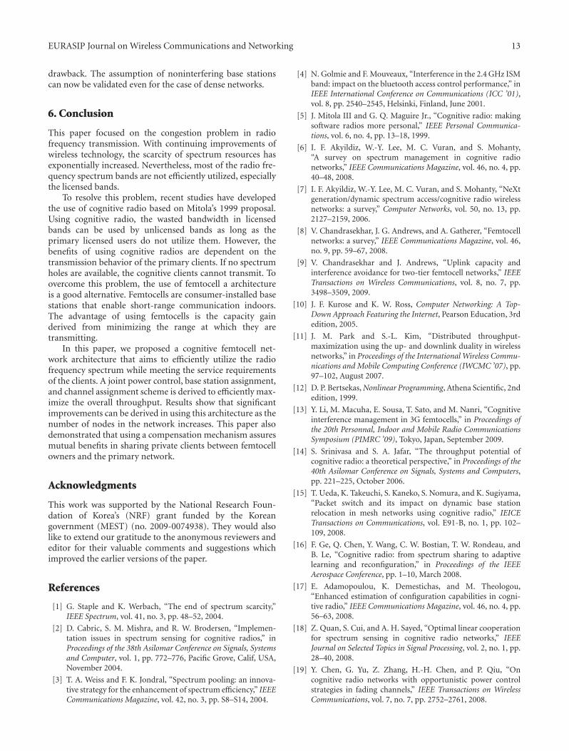
EURASIP Journal on Wireless Communications and Networking 13
drawback. The assumption of noninterfering base stationscan now be validated even for the case of dense networks.
6. Conclusion
This paper focused on the congestion problem in radiofrequency transmission. With continuing improvements ofwireless technology, the scarcity of spectrum resources hasexponentially increased. Nevertheless, most of the radio fre-quency spectrum bands are not efficiently utilized, especiallythe licensed bands.
To resolve this problem, recent studies have developedthe use of cognitive radio based on Mitola’s 1999 proposal.Using cognitive radio, the wasted bandwidth in licensedbands can be used by unlicensed bands as long as theprimary licensed users do not utilize them. However, thebenefits of using cognitive radios are dependent on thetransmission behavior of the primary clients. If no spectrumholes are available, the cognitive clients cannot transmit. Toovercome this problem, the use of femtocell a architectureis a good alternative. Femtocells are consumer-installed basestations that enable short-range communication indoors.The advantage of using femtocells is the capacity gainderived from minimizing the range at which they aretransmitting.
In this paper, we proposed a cognitive femtocell net-work architecture that aims to efficiently utilize the radiofrequency spectrum while meeting the service requirementsof the clients. A joint power control, base station assignment,and channel assignment scheme is derived to efficiently max-imize the overall throughput. Results show that significantimprovements can be derived in using this architecture as thenumber of nodes in the network increases. This paper alsodemonstrated that using a compensation mechanism assuresmutual benefits in sharing private clients between femtocellowners and the primary network.
Acknowledgments
This work was supported by the National Research Foun-dation of Korea’s (NRF) grant funded by the Koreangovernment (MEST) (no. 2009-0074938). They would alsolike to extend our gratitude to the anonymous reviewers andeditor for their valuable comments and suggestions whichimproved the earlier versions of the paper.
References
[1] G. Staple and K. Werbach, “The end of spectrum scarcity,”IEEE Spectrum, vol. 41, no. 3, pp. 48–52, 2004.
[2] D. Cabric, S. M. Mishra, and R. W. Brodersen, “Implemen-tation issues in spectrum sensing for cognitive radios,” inProceedings of the 38th Asilomar Conference on Signals, Systemsand Computer, vol. 1, pp. 772–776, Pacific Grove, Calif, USA,November 2004.
[3] T. A. Weiss and F. K. Jondral, “Spectrum pooling: an innova-tive strategy for the enhancement of spectrum efficiency,” IEEECommunications Magazine, vol. 42, no. 3, pp. S8–S14, 2004.
[4] N. Golmie and F. Mouveaux, “Interference in the 2.4 GHz ISMband: impact on the bluetooth access control performance,” inIEEE International Conference on Communications (ICC ’01),vol. 8, pp. 2540–2545, Helsinki, Finland, June 2001.
[5] J. Mitola III and G. Q. Maguire Jr., “Cognitive radio: makingsoftware radios more personal,” IEEE Personal Communica-tions, vol. 6, no. 4, pp. 13–18, 1999.
[6] I. F. Akyildiz, W.-Y. Lee, M. C. Vuran, and S. Mohanty,“A survey on spectrum management in cognitive radionetworks,” IEEE Communications Magazine, vol. 46, no. 4, pp.40–48, 2008.
[7] I. F. Akyildiz, W.-Y. Lee, M. C. Vuran, and S. Mohanty, “NeXtgeneration/dynamic spectrum access/cognitive radio wirelessnetworks: a survey,” Computer Networks, vol. 50, no. 13, pp.2127–2159, 2006.
[8] V. Chandrasekhar, J. G. Andrews, and A. Gatherer, “Femtocellnetworks: a survey,” IEEE Communications Magazine, vol. 46,no. 9, pp. 59–67, 2008.
[9] V. Chandrasekhar and J. Andrews, “Uplink capacity andinterference avoidance for two-tier femtocell networks,” IEEETransactions on Wireless Communications, vol. 8, no. 7, pp.3498–3509, 2009.
[10] J. F. Kurose and K. W. Ross, Computer Networking: A Top-Down Approach Featuring the Internet, Pearson Education, 3rdedition, 2005.
[11] J. M. Park and S.-L. Kim, “Distributed throughput-maximization using the up- and downlink duality in wirelessnetworks,” in Proceedings of the International Wireless Commu-nications and Mobile Computing Conference (IWCMC ’07), pp.97–102, August 2007.
[12] D. P. Bertsekas, Nonlinear Programming, Athena Scientific, 2ndedition, 1999.
[13] Y. Li, M. Macuha, E. Sousa, T. Sato, and M. Nanri, “Cognitiveinterference management in 3G femtocells,” in Proceedings ofthe 20th Personnal, Indoor and Mobile Radio CommunicationsSymposium (PIMRC ’09), Tokyo, Japan, September 2009.
[14] S. Srinivasa and S. A. Jafar, “The throughput potential ofcognitive radio: a theoretical perspective,” in Proceedings of the40th Asilomar Conference on Signals, Systems and Computers,pp. 221–225, October 2006.
[15] T. Ueda, K. Takeuchi, S. Kaneko, S. Nomura, and K. Sugiyama,“Packet switch and its impact on dynamic base stationrelocation in mesh networks using cognitive radio,” IEICETransactions on Communications, vol. E91-B, no. 1, pp. 102–109, 2008.
[16] F. Ge, Q. Chen, Y. Wang, C. W. Bostian, T. W. Rondeau, andB. Le, “Cognitive radio: from spectrum sharing to adaptivelearning and reconfiguration,” in Proceedings of the IEEEAerospace Conference, pp. 1–10, March 2008.
[17] E. Adamopoulou, K. Demestichas, and M. Theologou,“Enhanced estimation of configuration capabilities in cogni-tive radio,” IEEE Communications Magazine, vol. 46, no. 4, pp.56–63, 2008.
[18] Z. Quan, S. Cui, and A. H. Sayed, “Optimal linear cooperationfor spectrum sensing in cognitive radio networks,” IEEEJournal on Selected Topics in Signal Processing, vol. 2, no. 1, pp.28–40, 2008.
[19] Y. Chen, G. Yu, Z. Zhang, H.-H. Chen, and P. Qiu, “Oncognitive radio networks with opportunistic power controlstrategies in fading channels,” IEEE Transactions on WirelessCommunications, vol. 7, no. 7, pp. 2752–2761, 2008.

14 EURASIP Journal on Wireless Communications and Networking
[20] S. Geirhofer, L. Tong, and B. M. Sadler, “Cognitive mediumaccess: constraining interference based on experimental mod-els,” IEEE Journal on Selected Areas in Communications, vol. 26,no. 1, pp. 95–105, 2008.
[21] J. O. Neel, R. Menon, A. B. MacKenzie, J. H. Reed, and R.P. Gilles, “Interference reducing networks,” in Proceedings ofthe 2nd International Conference on Cognitive Radio OrientedWireless Networks and Communications (CrownCom ’07), pp.96–104, Orlando, Fla, USA, August 2007.
[22] H. Claussen, L. T. W. Ho, and L. G. Samuel, “Self-optimization of coverage for femtocell deployments,” inProceedings of the 7th Annual Wireless TelecommunicationsSymposium (WTS ’08), pp. 278–285, Ponoma, Calif, USA,April 2008.
[23] S. B. Kang, Y. M. Seo, Y. K. Lee, et al., “Soft QoS-based CACscheme for WCDMA femtocell networks,” in Proceedings ofthe 10th International Conference on Advanced CommunicationTechnology (ICACT ’08), vol. 1, pp. 409–412, February 2008.

Hindawi Publishing CorporationEURASIP Journal on Wireless Communications and NetworkingVolume 2010, Article ID 391684, 10 pagesdoi:10.1155/2010/391684
Research Article
A Bayesian Game-Theoretic Approach for Distributed ResourceAllocation in Fading Multiple Access Channels
Gaoning He,1 Merouane Debbah,2 and Eitan Altman3
1 Motorola Labs, Parc Les Algorithmes, 91193 Gif sur Yvette, France2 Alcatel-Lucent Chair on Flexible Radio, 3 Rue Joliot-Curie, 91192 Gif sur Yvette, France3 INRIA, 2004 Route des Lucioles, 06902 Sophia Antipolis, France
Correspondence should be addressed to Gaoning He, [email protected]
Received 31 August 2009; Revised 7 January 2010; Accepted 13 March 2010
Academic Editor: Ozgur Oyman
Copyright © 2010 Gaoning He et al. This is an open access article distributed under the Creative Commons Attribution License,which permits unrestricted use, distribution, and reproduction in any medium, provided the original work is properly cited.
A Bayesian game-theoretic model is developed to design and analyze the resource allocation problem in K-user fading multipleaccess channels (MACs), where the users are assumed to selfishly maximize their average achievable rates with incompleteinformation about the fading channel gains. In such a game-theoretic study, the central question is whether a Bayesian equilibriumexists, and if so, whether the network operates efficiently at the equilibrium point. We prove that there exists exactly one Bayesianequilibrium in our game. Furthermore, we study the network sum-rate maximization problem by assuming that the userscoordinate according to a symmetric strategy profile. This result also serves as an upper bound for the Bayesian equilibrium.Finally, simulation results are provided to show the network efficiency at the unique Bayesian equilibrium and to compare it withother strategies.
1. Introduction
The fading multiple access channel (MAC) is a basic wirelesschannel model that allows several transmitters connected tothe same receiver to transmit over it and share its capacity.The capacity region of the fading MAC and the optimalresource allocation algorithms have been characterized andwell studied in many pioneering works with different infor-mation assumptions [1–4]. However, in order to achieve thefull capacity region, it usually requires a central computingresource (a scheduler with comprehensive knowledge ofthe network information) to globally allocate the systemresources. This process is centralized, since it involvesfeedback and overhead communication whose load scaleslinearly with the number of transmitters in the network.In addition, with the fast evolution of wireless techniques,this centralized network infrastructure begins to expose itsweakness in many aspects, for example, slow reconfigura-tion against varying environment, increased computationalcomplexity, and so forth. This is especially crucial for femto-cell networks where it is quite difficult to centralize theinformation due to a limited capacity backhaul. Moreover,
the high density of base stations would increase the cost ofcentralizing the information.
In recent years, increased research interest has beengiven to self-organizing wireless networks in which mobiledevices allocate resources in a decentralized manner [5].Tools from game theory [6] have been widely applied tostudy the resource allocation and power control problemsin fading MAC [7], as well as many other types of channels,such as orthogonal frequency division multiplexing (OFDM)[8], multiple input and multiple output (MIMO) channels[9, 10], and interference channels [11]. Typically, the game-theoretic models used in these previous works assume thatthe knowledge, for example, channel state information (CSI),about other devices is available to all devices. However, thisassumption is hardly met in practice. In practical wirelessscenarios, mobile devices can have local information but canbarely access to global information on the network status.
A static noncooperative game has been introducedin the context of the two-user fading MAC, known as“waterfilling game” [7]. By assuming that users compete withtransmission rates as utility and transmit powers as moves,the authors show that there exists a unique Nash equilibrium

2 EURASIP Journal on Wireless Communications and Networking
[12] which corresponds to the maximum sum-rate pointof the capacity region. This claim is somewhat surprising,since the Nash equilibrium is in general inefficient comparedto the Pareto optimality. However, their results rely on thefact that both transmitters have complete knowledge of theCSI, and in particular, perfect CSI of all transmitters in thenetwork. As we previously pointed out, this assumption israrely realistic in practice.
Thus, this power allocation game needs to be recon-structed with some realistic assumptions made about theknowledge level of mobile devices. Under this consideration,it is of great interest to investigate scenarios in which deviceshave “incomplete information” about their components, forexample, a device is aware of its own channel gain, butunaware of the channel gains of other devices. In gametheory, a strategic game with incomplete information iscalled a “Bayesian game.” Over the last ten years, Bayesiangame-theoretic tools have been used to design distributedresource allocation strategies only in a few contexts, forexample, CDMA networks [13, 14], multicarrier interferencenetworks [15]. The primary motivation of this paper istherefore to investigate how Bayesian games can be appliedto study the resource allocation problems in the fadingMAC. In some sense, this study can help to design a self-organizing femto-cell network where different frequencybands or subcarriers are used for the femto-cell coverage, forexample, different femto-cells operate on different frequencybands to avoid interference.
In this paper, we introduce a Bayesian game-theoreticmodel to design and analyze the resource allocation problemin a fading MAC, where users are assumed to selfishly max-imize their ergodic capacity with incomplete informationabout the fading channel gains. In such a game-theoreticstudy, the central question is whether a Bayesian equilibriumexists, and if so, whether the network operates efficiently atthe equilibrium point. We prove that there exists exactly oneBayesian equilibrium in our game. Furthermore, we studythe network sum-rate maximization problem by assumingthat all users coordinate to an optimization-based symmetricstrategy. This centralized strategy is important when thefading processes for all users are relatively stationary and theglobal system structure is fixed for a long period of time. Thisresult also serves as an upper bound for the unique Bayesianequilibrium.
The paper is organized in the following form: InSection 2, we introduce the system model and state impor-tant assumptions. In Section 3, the K-user MAC is formu-lated as a static Bayesian game. In Section 4, we charac-terize the Bayesian equilibrium set. In Section 5, we give aspecial discussion on the optimal symmetric strategy. Somenumerical results are provided to show the efficiency of theBayesian equilibrium in Section 6. Finally, we close withsome concluding remarks in Section 7.
2. System Model and Assumptions
2.1. System Model. We consider the uplink of a single-cell network where K users are simultaneously sending
information to one base station. This corresponds to a fadingMAC, in which the users are the transmitters and the basestation is the receiver. The signal received at the base stationcan be mathematically expressed as
y(t) =K∑
k=1
√gk(t)xk(t) + z(t), (1)
where xk(t) and gk(t) are the input signal and fading channelgain of user k, and z(t) is a zero-mean white Gaussiannoise with variance σ2. The input signal xk(t) can be furtherwritten as
xk(t) =√pk(t)sk(t), (2)
where pk(t) and sk(t) are the transmitted power and data ofuser k at time t.
In this study, we consider the wireless transmissionin fast fading environments, that is, the coherence timeof the channel is small relative to the delay constraint ofthe application. When the receiver can perfectly track thechannel but the transmitters have no such information, thecodewords cannot be chosen as a function of the state of thechannel but the decoding can make use of such information.When the fading process is assumed to be stationary andergodic within the considered interval of signal transmission,the channel capacity in a fast fading channel corresponds tothe notion of ergodic capacity, that is,
Eg
⎡
⎣log
⎛
⎝1 +gk pk
σ2 +∑K
j=1, j /= k gj p j
⎞
⎠
⎤
⎦, (3)
where g = {g1, . . . , gK} is a vector of channel gain variables.Note that in (3) we assume that the receiver applies asingle-user decoding and there is not sophisticated successivedecoding to be used. An intuitive understanding of thisresult can be obtained by viewing capacities in terms oftime averages of mutual information [16]. Although thestudy of multiuser decoding is important, which may involveStackelberg games, fairness concepts, and generalized Nashgames, it is not provided in this study. The interested readersare referred to [17] for this topic.
2.2. Assumption of Finite Channel States. Before introducingour game model, we need to clarify a prior assumption forthis section.
Assumption 1. We assume that each user’s channel gain gkis i.i.d. from two discrete values: g− and g+ with probabilityρ− and ρ+, respectively. Without loss of generality, we assumeg− < g+.
On the one hand, our assumption is closely relatedto the way how feedback information is signalled to thetransmitters. In order to get the channel information gk atthe transmitter side, the base station is required to feedbackan estimate of gk to user k at a given precision. Since in digitalcommunications, any information is represented by a finite

EURASIP Journal on Wireless Communications and Networking 3
number of bits (e.g., x bits), channels gains are mapped intoa set that contains a finite number of states (2x states).
On the other hand, this is a necessary assumptionfor analytical tractability, since in principle the functionalstrategic form of a player can be quite complex with bothactions and states being continuous (or infinite). To avoidthis problem, in [15] the authors successfully modelled amulticarrier Gaussian interference channel as a Bayesiangame with discrete (or finite) actions and continuous states.Inspired from [15], we also model the fading MAC as aBayesian game under the assumption of continuous actionsand discrete states.
3. Game Formulation
We model the K-user fading MAC as a Bayesian game, inwhich users do not have complete information. In a K-user MAC, to have “complete information” means that, ateach time t, the channel gain realizations g1(t), . . . , gK (t) areknown at all the transmitters, denoted by Tx1, . . . , TxK . Anyother condition corresponds to a situation of incompleteinformation. In this paper, the “incomplete information”particularly refers to a situation where each Txk onlyknows its own channel gain realization gk(t), but does notknow the channel gains of other transmitters g−k(t) ={g1(t), . . . , gk−1(t), gk+1(t), . . . , gK (t)}. We will denote by gkthe channel gain variable of user k, whose distribution isassumed to be stationary and ergodic in this section.
In such a communication system, the natural object ofeach user is to maximize its ergodic capacity subject to anaverage power constraint, that is,
maxpk
Eg
⎡
⎣log
⎛
⎝1 +gk pk
(gk)
σ2 +∑
j /= k gj p j(gj)
⎞
⎠
⎤
⎦
s.t. Egk[pk(gk)] ≤ Pmax
k
pk(gk) ≥ 0,
(4)
where pk(·) and Pmaxk are transmit power strategy and
average power constraint of user k, respectively. Under theassumption that each user has incomplete information aboutthe channel gains, user k’s strategy pk(·) is defined as afunction of its own channel gain gk, that is, pk(gn). Note that(4) implies that user k should know at least the statistics ofother users’ channels.
For a given set of power strategies p−k = {p1, . . .,pk−1, pk+1, . . . , pK}, the single-user maximization problem(4) is a convex optimization problem [18]. Via Lagrangianduality, the solution is given by the following equation:
Eg−k
⎡
⎣ gk
σ2 + gk pk(gk)
+∑
j /= k gj p j(gj)
⎤
⎦ = λk, (5)
where the dual variable λk is chosen such that the powerconstraint in (4) is satisfied with equality. However, thesolution of (5) depends on p−k(·) which user k does not
know, and the same holds for all other users. Thus, in orderto obtain the optimal power allocation, each user must adjustits power level based on the guess of all other users’ strategies.Now, given the following game model, each user is able toadjust its strategy according to the belief it has about thestrategy of the other user.
The K-player MAC Bayesian game can be completelycharacterized as
GMAC � 〈K , T , P , Q, U〉. (6)
(i) Player set: K = {1, . . . ,K}.(ii) Type set: T = T1 × · · · × TK (“×” stands for the
Cartesian product) where Tk = {g−, g+}. A player’stype is defined as its channel gain, that is, gk ∈ Tk.
(iii) Action set: P = P1×· · ·×PK where Pk = [0,Pmaxk ].
A player’s action is defined as its transmit power, thatis, pk ∈ Pk.
(iv) Probability set: Q = Q1 × · · · × QK where Qk ={ρ−, ρ+}, we have ρ+ = Pr(gk = g+) and ρ− = Pr(gk =g−).
(v) Payoff function set: U = {u1, . . . ,uK} where uk ischosen as player k’s achievable rate
uk(p1, . . . , pK
) = log
⎛
⎝1 +gk pk
(gk)
σ2 +∑K
j=1, j /= k gj p j(gj)
⎞
⎠.
(7)
In games of incomplete information, a player’s typerepresents any kind of private information that is relevantto its decision making. In our context, the fading channelgain gk is naturally considered as the type of user k, sinceits decision (in terms of power) can only rely on gk. Notethat this is a continuous game (a continuous game extends thenotion of a discrete game (where players choose from a finiteset of pure strategies), it allows players to choose a strategyfrom a continuous pure strategy set) with discrete states,since each player’s action pk can take any value satisfying theconstraint pk ∈ [0, Pmax
k ] and the channel state gk is finitegk ∈ {g−, g+}.
4. Bayesian Equilibrium
4.1. Definition of Bayesian Equilibrium. What we can expectfrom the outcome of a Bayesian game if every selfish andrational (rational player means a player chooses the bestresponse given its information) participant starts to playthe game? Generally speaking, the process of such players’behaviors usually results in a Bayesian equilibrium, whichrepresents a common solution concept for Bayesian games.In many cases, it represents a “stable” result of learning andevolution of all participants. Therefore, it is important tocharacterize such an equilibrium point, since it concerns theperformance prediction of a distributed system.

4 EURASIP Journal on Wireless Communications and Networking
Now, let { pk(·), p−k(·)} denote the strategy profile whereall players play p(·) except player k who plays pk(·), we canthen describe player k’s payoff as
uk(pk, p−k
) = uk(p1, . . . , pk−1, pk, pk+1, . . . , pK
). (8)
Definition 2 (Bayesian equilibrium). The strategy profilep�(·) = {p�k (·)}k∈K is a (pure strategy) Bayesian equilib-rium, if for all k ∈ K , and for all pk(·) ∈ Pk and p−k(·) ∈P−k
uk(p�k , p�−k
)≥ uk
(pk, p�−k
), (9)
where we define un � Eg[uk].
From this definition, it is clear that at the Bayesianequilibrium no player can benefit from changing its strategywhile the other players keep theirs unchanged. Note that in astrategic-form game with complete information each playerchooses a concrete action, whereas in a Bayesian game eachplayer k faces the problem of choosing a set or collection ofactions (power strategy pk(·)), one for each type (channelgain gk) it may encounter. It is also worth to mention that theaction set of each player is independent of the type set, thatis, the actions available to user k are the same for all types.
4.2. Characterization of the Bayesian Equilibrium Set. It iswell known that, in general, an equilibrium point does notnecessarily exist [6]. Therefore, our primary interest in thispaper is to investigate the existence and uniqueness of aBayesian equilibrium in GMAC. We now state our main result.
Theorem 3. There exists a unique Bayesian equilibrium in theK-user MAC game GMAC.
Proof. It is easy to prove the existence part, since the strategyspace pk is convex, compact, and nonempty for each k; thepayoff function uk is continuous in both pk and p−k; uk isconcave in pk for any p−k [6].
In order to prove the uniqueness part, we should rely ona sufficient condition given in [19]: a non-cooperative gamehas a unique equilibrium, if the nonnegative weighted sumof the payoff functions is diagonally strictly concave. We firstlygive the definition.
Definition 4 (diagonally strictly concave). A weighted non-negative sum function f (x, r) = ∑n
i=1 riϕi(x) is calleddiagonally strictly concave for any vector x ∈ Rn×1 and fixedvector r ∈ Rn×1
++ , if for any two different vectors x0, x1, wehave
Ω(
x0, x1, r)
�(
x1 − x0)Tδ(
x0, r)
+(
x0 − x1)Tδ(
x1, r)> 0,(10)
where δ(x, r) is called pseudogradient of f (x, r), defined as
δ(x, r) �
⎡
⎢⎢⎢⎢⎢⎢⎢⎣
r1∂ϕ1
∂x1...
rn∂ϕn∂xn
⎤
⎥⎥⎥⎥⎥⎥⎥⎦
. (11)
We start with the following lemma.
Lemma 5. The weighted nonnegative sum of the averagepayoffs uk in GMAC is diagonally strictly concave for r = c+1,where c+ is a positive scalar, 1 is a vector whose every entry is 1.
Proof. Write the weighted nonnegative sum of the averagepayoffs as
f u(
p, r)
�K∑
k=1
rkuk(
p), (12)
where p = [p1 · · · pK ]T is the transmit power vector andr = [r1 · · · rK ]T is a nonnegative vector assigning weightsr1, . . . , rK to the average payoffs u1, . . . ,uK , respectively. Sim-ilar to (11), we let δu(p, r) � [r1(∂u1/∂p1) . . . rK (∂uK/∂pK )]T
be the pseudogradient of f u(p, r). Now, we define
pk � pk(g−) ∀k, (13)
the transmit power of player k when its channel gain isg−. Since we have shown from the Lagrangian that, at theequilibrium, the power constraint is satisfied with equality,that is, Egk [pk(gk)] = Pmax
k , we can write Pmaxk − ρ−pk(g−) =
ρ+pk(g+) for all k, as the transmit power when its channelgain is g+. Therefore, it is easy to find that the average payoffuk can be actually transformed into a weighted sum-logfunction as follows:
uk(pk) =
∑
i
ωi log
⎡
⎣1 +αik + βik pk
σ2 +∑
j /= k(αij + βij p j
)
⎤
⎦, (14)
where i represents the index for different jointly probabilityevents, ωi represents the corresponding probability for eventi that are related to the probabilities {ρ−, ρ+}, and αik and βinrepresent some positive and nonzero real numbers that arerelated to the channel gains {g−, g+}. Note that the followingconditions hold for all i, k:
ωi > 0, αik + βik pk ≥ 0, αik > 0, βik /= 0, σ2 > 0.(15)
Now, we can write the pseudogradient δu as
δu(
p, r) =
⎡
⎢⎢⎢⎢⎢⎢⎣
c+ ∂u1
∂p1...
c+ ∂uK∂pK
⎤
⎥⎥⎥⎥⎥⎥⎦
=
⎡
⎢⎢⎢⎢⎢⎢⎢⎣
c+∑
i
ωiβi1φ−1i
(p)
...
c+∑
i
ωiβiKφ
−1i
(p)
⎤
⎥⎥⎥⎥⎥⎥⎥⎦
= c+∑
i
⎡
⎢⎢⎣
ωiβi1φ−1i
(p)
...ωiβ
iKφ
−1i
(p)
⎤
⎥⎥⎦,
(16)

EURASIP Journal on Wireless Communications and Networking 5
where the function φi(x) is defined as
φi(x) � σ2 +K∑
k=1
(αik + βik xk
). (17)
To check the diagonally strictly concave condition (10), we letp0, p1 be two different vectors satisfying the power constraint,and define
Ωu(
p0, p1, r)
�(
p1 − p0)Tδu(
p0, r)
+(
p0 − p1)Tδu(
p1, r)
= (p1 − p0)T[δu(
p0, r)− δu(p1, r
)]
= [Δp1 · · · ΔpK]
×
⎡
⎢⎢⎢⎢⎢⎢⎣
c+∑
i
ωiβi1
(φ−1i
(p0)− φ−1
i
(p1))
...c+∑
i
ωiβiK
(φ−1i
(p0)− φ−1
i
(p1))
⎤
⎥⎥⎥⎥⎥⎥⎦
= c+∑
i
ωi[φ−1i
(p0)− φ−1
i
(p1)]ζi
= c+∑
i
ωiφ−1i
(p0)φ−1
i
(p1)ζ2
i ,
(18)
where Δpk and ζi are defined as
Δpk � p1k − p0
k ,
ζi �K∑
k=1
βikΔpk,(19)
Since p0, p1 are assumed to be two different vectors, wemust have Δp = [Δp1 · · ·ΔpK ]T
/= 0. Now, we can draw aconclusion from the equation above:Ωu(p0, p1, r) > 0. This isbecause: (1) the first partωiφ−1
i (p0)φ−1i (p1) > 0 for all i, since
ωi > 0, σ2 > 0 and αik + βik pk ≥ 0 for all i, k; (2) the secondpart ζ2
i ≥ 0 for all i, and there exists at least one nonzero termζ2i , due to Δp /= 0 and rk /= 0, βik /= 0 for all i, k. Therefore,
the summation of all the products of the first and the secondterms must be positive. From Definition 4, the sum-payofffunction f u(p, r) satisfies the condition of diagonally strictlyconcave. This completes the proof of this lemma.
Since our sum-payoff function f u(p, r) given in (12)is diagonally strictly concave, the uniqueness of Bayesianequilibrium in our game GMAC follows directly from [19,Theorem 2].
5. Optimal Symmetric Strategies
The Bayesian game-theoretic approach provides us a betterunderstanding of the wireless resource competition existingin the fading MAC when every mobile device acts as aselfish and rational decision maker (this means a devicealways chooses the best response given its information).The advantage of this model is that it mathematically
captures the behavior of selfish wireless entities in strategicsituations, which can automatically lead to the convergenceof system performance. The introduced Bayesian game-theoretic framework fits very well the concept of self-organizing networks, where the intelligence and decisionmaking is distributed. Such a scheme has apparent benefitsin terms of operational complexity and feedback load.
However, from the global system performance perspec-tive, it is usually inefficient to give complete “freedom”to mobile devices and let them take decisions withoutany policy control over the network. It is very interestingto note that a similar situation happens in the marketeconomy, where consumers can be modeled as players tocomplete for the market resources. In the famous literatureThe Wealth of Nations, Adam Smith (a Scottish moralphilosopher, pioneer of political economy, and father ofmodern economics) expounded how rational self-interestand competition can lead to economic prosperity and well-being through macroeconomic adjustments. For example, allstates today have some form of macroeconomic control overthe market that removes the free and unrestricted directionof resources from consumers and prices such as tariffs andcorporate subsidies.
In particular, wireless service providers would like todesign an appropriate policy to efficiently manage the systemresource so that the global network performance can beoptimized or enhanced to a certain theoretical limit, forexample, Shannon capacity or capacity region [20]. Appar-ently, a centralized scheduler with comprehensive knowledgeof the network status can globally optimize the resourceutility. However, this approach usually involves sophisticatedoptimization techniques and a feedback load that grows withthe number of wireless devices in the network. Thus, theoptimization-based centralized decision has to be frequentlyupdated as long as the wireless environment varies, or thesystem structure changes, for example, a user joins or exitsthe network.
In this section, we consider that the channel statistics(fading processes) for all wireless devices are jointly station-ary for a relatively long period of signal transmission, andthe global system structure remains unchanged. In addition,we neglect the problem of computational complexity at thescheduler and the impact of feedback load to the useful datatransmission rate. In this case, the network service providerwould strictly prefer to use a centralized approach, that is,a scheduler assigns some globally optimal strategies to thewireless devices, guiding them how to react under all kindsof different situations. Based on the Bayesian game settings,we provide a special discussion on the optimal symmetricstrategy design. Note that this result can be treated as atheoretical upperbound for the performance measurementof Bayesian equilibrium.
We now introduce a necessary assumption.
Assumption 6. Mobile devices are designed to use the samepower strategies, that is, they send the same power iftheir observations on the channel states are symmetric. Inaddition, we assume that the mobile devices have the sameaverage power constraint, that is, Pmax
1 = · · · = PmaxK � Pmax.

6 EURASIP Journal on Wireless Communications and Networking
5.1. Two Channel States. For simplicity of our presentation,We first consider the scenario of two users with two channelstates. In fact, the analysis of multiuser MAC can be extendedin a similar way. According to Assumption 6, we define
p− � p1(g−) = p2
(g−),
p+ � p1(g+) = p2
(g+),
(20)
and we have ρ−p− + ρ+p+ = Pmax. Write user 1’s averagepayoff as (Without loss of generality, we consider user 1 in thefollowing context, since the problem is symmetric for user 2)
u1 = Eg1,g2
[
log2
(
1 +g1p1
(g1)
σ2 + g2p2(g2)
)]
= ρ2−log2
(
1 +g−p−
σ2 + g−p−
)
+ ρ−ρ+log2
(
1 +g−p−
σ2 + g+(Pmax − ρ−p−
)/ρ+
)
+ ρ−ρ+log2
(
1 +g+(Pmax − ρ−p−
)/ρ+
σ2 + g−p−
)
+ ρ2+log2
(
1 +g+(Pmax − ρ−p−
)/ρ+
σ2 + g+(Pmax − ρ−p−
)/ρ+
)
.
(21)
Now, u1 is transformed into a function of p−, write it asu1(p−). To maximize the average achievable rate, user 1 needsto solve the following optimization problem, as mentioned in(4)
maxp−
u1(p−)
s.t. 0 ≤ p− ≤ Pmax
ρ−.
(22)
Under Assumption 6, it can be shown that (due to thesymmetric property) this single-user maximization problemis equivalent to the multiuser sum average rate maximizationproblem, that is, max(u1 + u2), which is our object in thissection.
But unfortunately, u1 may not be a convex function [18],so the single-user problem may not be a convex optimizationproblem. It can be further verified that u1 is convex undersome special conditions, depending on all the parametersg−, g+, ρ−, ρ+,Pmax, and σ2. Here, we will not discuss allthe convex cases, but only focus on the high SNR regime(meaning that the noise can be omitted compared to thesignal strength). In this case, we have
limσ2 → 0
u1 = ρ−ρ+
[
log2
(
1 +g−p−
g+(Pmax − ρ−p−
)/ρ+
)
+log2
(
1 +g+(Pmax − ρ−p−
)/ρ+
g−p−
)]
+ ρ2− + ρ2
+.
(23)
This function is strict convex. To be more precise, it isdecreasing on [0, g+Pmax/(g−ρ+ + g+ρ−)) and increasing on(g+Pmax/(g−ρ+ + g+ρ−),Pmax/ρ−], and the solution is givenby
{p�− , p�+
} =
⎧⎪⎪⎪⎪⎪⎨
⎪⎪⎪⎪⎪⎩
{
0,Pmax
ρ+
}
,g+
ρ+≥ g−ρ−
,
{Pmax
ρ−, 0
}
,g+
ρ+<g−ρ−.
(24)
Note that in this setting the choice of the optimalsymmetric strategy is to concentrate the full available poweron a single channel state. The selection of the channel stateon which to transmit depends not only on the channelconditions but also on the probability of the channel states.This result implies that, in the high SNR regime, theoptimal symmetric power strategy is to transmit informationin an “opportunistic” way. For a better understanding ofthe “opportunistic” transmission, the interested reads arereferred to [2].
5.2. Multiple Channel States. In this subsection, we discussthe extension to arbitrary L (L ≥ 2) channel states. Note thatthe result of this subsection can also be applied to the case oftwo channel states.
Assumption 7. Each user’s channel gain gk has L positivestates, which are a1, . . . , aL with probability ρ1, . . . , ρL, respec-tively (Without loss of generality,a1 < · · · < aL), and we have∑L
=1 ρ = 1.
Based on Assumption 6, we define p � p1(a ) =p2(a ), = 1, . . . ,L, as the transmit power when a user’schannel gain is a . As previously mentioned, our object inthis part is to maximize the sum ergodic capacity of thesystem, that is, max
∑k uk. Under the symmetric assumption,
this sum-ergodic-capacity maximization problem is equiva-lent to the following single-user maximization problem
maxp
∑
i
∑
j
ρiρ j log2
(
1 +gi pi
σ2 + gj p j
)
s.t.∑
i
ρi pi ≤ Pmax
pi ≥ 0, i = 1, . . . ,L,
(25)
where p is now defined as p = {p1, . . . , pL}. This optimiza-tion problem is difficult, since the objective function is againnonconvex in p. However, we can consider a relaxation of theoptimization by introducing a lower bound [21]
α log z + β ≤ log(1 + z), (26)
where α and β are chosen specified as
α = z0
1 + z0,
β = log(1 + z0)− z0
1 + z0log z0,
(27)

EURASIP Journal on Wireless Communications and Networking 7
we say that the lower bound (26) is tight with equality at achosen value z0.
Let us consider the lower bound (denoted as ξ) by usingthe relaxation (26) to the objective function in (25)
ξ(
p)
�∑
i
∑
j
ρiρ j
[
αi, j log2
(gi pi
σ2 + gj p j
)
+ βi, j
]
(28)
which is still nonconvex, and so it is not concave inp. However, with a logarithmic change of the followingvariables and constants: pi = log2 pi, pi = log2 pi andgi = log2 gi, we can turn the geometric programming [18]associated with the objective function (28) into the followingproblem:
maxp
ξ(
p)
s.t.∑
i
ρi2 pi ≤ Pmax,(29)
where ξ(p) is defined as
ξ(
p) =
∑
i
∑
j
ρiρ jαi, j(gi + pi
)
−∑
i
∑
j
ρiρ jαi, j log2
(σ2 + 2(g j+ p j )
)
+∑
i
∑
j
ρiρ jβi, j .
(30)
Now, it is easy to verify that the lower bound ξ is concavein the transformed set p, since the log-sum-exp function isconvex. The constraints of the optimization problem are suchthat Slater’s condition is satisfied [18]. So, the Karush-Kuhn-Tucker (KKT) condition of the optimization is sufficient andnecessary for the optimality. Given the following Lagrangiandual function (denoted by L):
L(
p, ν) =
∑
i
∑
j
ρiρ jαi, j(ai + pi
)
−∑
i
∑
j
ρiρ jαi, j log2
(σ2 + 2(a j+ p j )
)
+∑
i
∑
j
ρiρjβi, j − ν
⎛
⎝∑
i
2(ai+ pi) − Pmax
⎞
⎠,
(31)
the KKT conditions are
ρ ∑
j
ρ jα , j − ρ (
2(a + p )
σ2 + 2(a + p )
)
×∑
i
ρiαi, − (ν ln 2)2(a + p ) = 0, ∀ ,
(32)
where a = log2a , and ν ≥ 0 is a dual variable associatedwith the power constraint in (29).
Define x � 2(a + p ), = 1, . . . ,L, the equivalent KKTconditions can be simply written as a quadratic equation
A x2 + B x + C = 0, ∀ , (33)
where the parameters A ,B ,C are expressed as
A = ν ln 2, ∀
B = ρ ∑
i
ρi(αi, − α ,i
)+ σ2ν ln 2, ∀
C = −ρ σ2∑
i
ρiα ,i, ∀ .
(34)
Note that A and B are functions of ν, we can write themas A (ν) and B (ν). Since x ≥ 0, the solution to the KKTconditions can only be one of the roots to the quadraticequation, that is,
p� =−B (ν) +
√B2 (ν)− 4A (ν)C
2a A (ν), ∀ , (35)
where ν is chosen such that∑
ρ p� = Pmax. Thus, for some
fixed value of α,β, we can directly apply (35) to maximize thelower bound ξ (28). Then, it is natural to improve the boundperiodically. Based on the discussion above, we propose thefollowing algorithm, namely Lower Bound Tightening (LBT)algorithm
The algorithm convergence can be easily proved, sincethe objective is monotonically increasing at each iteration.However, the global optimum is not always guaranteed, dueto the nonconvex property.
6. Numerical Results
In this section, numerical results are presented to validateour theoretical claims. For Figures 1 and 2, the networkparameters are chosen as ρ− = ρ+ = 0.5, Pmax = 1 andσ2 = 0.1.
First, we show the existence and uniqueness of Bayesianequilibrium in the scenario of two-user fading MAC. InFigure 1(a), we assume the channel gains are g− = 1, g+ = 3;in Figure 1(b), we assume g− = 1, g+ = 10. On both X andY axis, p1 and p2 represent the power allocated by user 1 anduser 2 when the channel gain is g−. The curves r1(p2) andr2(p1) represent the best-response functions of user 1 anduser 2, respectively. As expected, the Bayesian equilibrium isunique in both cases, that is, (0.6,0.6) and (0.5,0.5).
Second, we investigate the efficiency of Bayesian equi-librium from the viewpoint of global average networkperformance. The X axis, SNR is defined as the ratiobetween the power constraint Pmax and the noise varianceσ2. In Figure 2(a), again, we assume g− = 1, g+ = 3;in Figure 2(b), we assume g− = 1, g+ = 10. The curve“Pareto” represents the Nash equilibrium in the waterfillinggame, in which users have complete information. This givesthe upper bound for our Bayesian equilibrium, since it isalso the Pareto optimal solution [7]. The curve “Uniform”

8 EURASIP Journal on Wireless Communications and Networking
0
0.2
0.4
0.6
0.8
1
1.2
1.4
1.6
1.8
2p 2
Nash equilibrium
0 0.5 1 1.5 2
p1
r2(p1)r1(p2)
(a)
0
0.2
0.4
0.6
0.8
1
1.2
1.4
1.6
1.8
2
p 2
Nash equilibrium
0 0.5 1 1.5 2
p1
r2(p1)r1(p2)
(b)
Figure 1: The uniqueness of Bayesian equilibrium. (a) g− = 1, g+ = 3, (b) g− = 1, g+ = 10.
0.5
1
1.5
2
2.5
3
3.5
Ave
rage
net
wor
ksu
m-r
ate
(bps
/Hz)
0 5 10 15 20 25 30
SNR (dB)
ParetoSymmetric
BayesianUniform
(a)
0.5
1
1.5
2
2.5
3
3.5
Ave
rage
net
wor
ksu
m-r
ate
(bps
/Hz)
0 5 10 15 20 25 30
SNR (dB)
ParetoSymmetric
BayesianUniform
(b)
Figure 2: Average network sum-rate. (a) g− = 1, g+ = 3, (b) g− = 1, g+ = 10.
represents the time-domain uniform power allocation. Sincethis is the strategy when users have no information aboutthe channel gains, it corresponds obviously to a lowerbound. The curve “Symmetric” represents the optimalsymmetric strategy presented in Section 5. This can betreated as a weaker upper bound (inferior to the Paretooptimality) for the Bayesian equilibrium. From the slopesof these curves, we can clearly observe the inefficiency ofthe Bayesian equilibrium, especially in the high SNR regime.This can be explained as follows: in our game GMAC, userswith incomplete information improve the global networkperformance (comparing to the scenario in which the users
have no information), however, it does not improve theperformance slope.
Finally, we show the convergence behavior of the lowerbound tightening (LBT) algorithm. In Figure 3, we choosethe parameters as L = 3, g1 = 1, g2 = 2, g3 = 3, and ρ1 =ρ2 = ρ3 = 1/3. The sum capacity versus the SNR areplotted for five iterations. The upper bound is achieved byexhaustive search. As expected, one can easily observe theconvergence behavior. In the low SNR regime, we can findthat the algorithm converges to the local instead of the globalmaximum. However, we also find that the performance of thelocal optimum is improved while the SNR is increasing.

EURASIP Journal on Wireless Communications and Networking 9
0.7
0.8
0.9
1
1.1
1.2
1.3
1.4
1.5
1.6
1.7
Ave
rage
net
wor
ksu
m-r
ate
(bps
/Hz)
0 2 4 6 8 10
SNR (dB)
Exhaustive searchIteration 5Iteration 4
Iteration 3Iteration 2Iteration 1
Figure 3: The convergence of the lower bound tightening (LBT)algorithm.
Initialize t = 0; ν = 0; α(t)i, j = 1, for i = 1, . . . ,L, j = 1, . . . ,L.
repeatrepeat
ν = ν + Δνfor i = 1 to L do
update Ai,Bi,Ci using (34)
p�i = (−Bi +√B2i − 4AiCi)/2aiAi
end foruntil
∑i ρi p
�i = Pmax
for i = 1 to L and j = 1 to L doz(t)i, j = ai p
�i /(σ
2 + aj p�j ); α(t+1)
i, j = z(t)i, j /(1 + z(t)
i, j )end fort = t + 1
until converge
Algorithm 1: Lower Bound Tightening (LBT).
7. Conclusion
We presented a Bayesian game-theoretic framework fordistributed resource allocation in fading MAC, where usersare assumed to have only information about their ownchannel gains. By introducing the assumption of finitechannel states, we successfully found a analytical way tocharacterize the Bayesian equilibrium set. First, we provedthe existence and uniqueness. Second, the inefficiency wasshown from numerical results. Furthermore, we analyzedthe optimal symmetric power strategy based on the prac-tical concerns of resource allocation design. Future exten-sion is considered to improve the efficiency of Bayesianequilibrium through pricing or cooperative game-theoreticapproaches.
References
[1] R. S. Cheng and S. Verdu, “Gaussian multiaccess channelswith ISI. Capacity region and multiuser water-filling,” IEEETransactions on Information Theory, vol. 39, no. 3, pp. 773–785, 1993.
[2] R. Knopp and P. A. Humblet, “Information capacity andpower control in single-cell multiuser communications,” inProceedings of IEEE International Conference on Communica-tions (ICC ’95), vol. 1, pp. 331–335, Seattle, Wash, USA, June1995.
[3] A. J. Goldsmith and P. P. Varaiya, “Capacity of fadingchannels with channel side information,” IEEE Transactions onInformation Theory, vol. 43, no. 6, pp. 1986–1992, 1997.
[4] D. N. C. Tse and S. V. Hanly, “Multiaccess fading channels—part I: polymatroid structure, optimal resource allocationand throughput capacities,” IEEE Transactions on InformationTheory, vol. 44, no. 7, pp. 2796–2815, 1998.
[5] M. Debbah, “Mobile flexible networks: the challenges ahead,”in Proceedings of the International Conference on AdvancedTechnologies for Communications (ATC ’08), pp. 3–7, Hanoi,Vietnam, October 2008.
[6] D. Fudenberg and J. Tirole, Game Theory, MIT Press, Cam-bridge, Mass, USA, 1991.
[7] L. Lai and H. El Gamal, “The water-filling game in fadingmultiple-access channels,” IEEE Transactions on InformationTheory, vol. 54, no. 5, pp. 2110–2122, 2008.
[8] G. He, S. Beta, and M. Debbah, “Game-theoretic deploymentdesign of small-cell OFDM networks,” in Proceedings of the3rd ICST/ACM International Workshop on Game Theory inCommunication Networks, October 2009.
[9] S. Lasaulce, M. Debbah, and E. Altman, “Methodologies foranalyzing equilibria in wireless games: a look at pure, mixed,and correlated equilibria,” IEEE Signal Processing Magazine,vol. 26, no. 5, pp. 41–52, 2009.
[10] E.-V. Belmega, S. Lasaulce, and M. Debbah, “Power allocationgames for mimo multiple access channels with coordination,”IEEE Transactions on Wireless Communications, vol. 8, no. 6,pp. 3182–3192, 2009.
[11] E. Altman, M. Debbah, and A. Silva, “Game theoreticapproach for routing in Dense ad-hoc networks,” in Proceed-ings of the Stochastic Networks Workshop, Edinburg, UK, July2007.
[12] J. F. Nash, “Equilibrium points in N-person games,” Proceed-ings of the National Academy of Sciences of the United States OfAmerica, vol. 36, no. 1, pp. 48–49, 1950.
[13] T. Heikkinen, “A minmax game of power control in a wirelessnetwork under incomplete information,” Tech. Rep. 99-43,DIMACS, August 1999.
[14] C. A. St. Jean and B. Jabbari, “Bayesian game-theoretic mod-eling of transmit power determination in a self-organizingCDMA wireless network,” in Proceedings of the 60th IEEEVehicular Technology Conference (VTC ’04), vol. 5, pp. 3496–3500, 2004.
[15] S. Adlakha, R. Johari, and A. Goldsmith, “Competi-tion in wireless systems via Bayesian interference games,”http://arxiv.org/abs/0709.0516.
[16] R. Gallager, “An inequality on the capacity region of multiac-cess fading channels,” in Communications and Cryptography:Two Sides of One Tapestry, pp. 129–139, Kluwer AcademicPublishers, Boston, Mass, USA, 1994.

10 EURASIP Journal on Wireless Communications and Networking
[17] E. Altman, K. Avrachenkov, L. Cottatellucci, M. Debbah, G.He, and A. Suarez, “Operating point selection in multipleaccess rate regions,” in Proceedings of the 21st InternationalTeletraffic Congress (ITC ’09), Paris, France, June 2009.
[18] S. Boyd and L. Vandenberghe, Convex Optimization, Cam-bridge University Press, Cambridge, UK, 2004.
[19] J. B. Rosen, “Existence and uniqueness of equilibrium pointsfor concave N-person games,” Econometrica, vol. 33, pp. 520–534, 1965.
[20] T. M. Cover and J. A. Thomas, Elements of Information Theory,Wiley, New York, NY, USA, 1991.
[21] J. Papandriopoulos and J. S. Evans, “Low-complexity dis-tributed algorithms for spectrum balancing in multi-user DSLnetworks,” in Proceedings of IEEE International Conference onCommunications (ICC ’06), vol. 7, pp. 3270–3275, June 2006.

Hindawi Publishing CorporationEURASIP Journal on Wireless Communications and NetworkingVolume 2010, Article ID 143413, 12 pagesdoi:10.1155/2010/143413
Research Article
Dynamic Resource Partitioning for DownlinkFemto-to-Macro-Cell Interference Avoidance
Zubin Bharucha,1 Andreas Saul,1 Gunther Auer,1 and Harald Haas2
1 DOCOMO Communications Laboratories Europe GmbH, Landsberger Straße 312, 80687 Munich, Germany2 School of Engineering and Electronics, Institute for Digital Communications, Joint Research Institute for Signal and Image Processing,The University of Edinburgh, Edinburgh EH9 3JL, UK
Correspondence should be addressed to Zubin Bharucha, [email protected]
Received 31 December 2009; Accepted 26 April 2010
Academic Editor: Holger Claussen
Copyright © 2010 Zubin Bharucha et al. This is an open access article distributed under the Creative Commons AttributionLicense, which permits unrestricted use, distribution, and reproduction in any medium, provided the original work is properlycited.
Femto-cells consist of user-deployed Home Evolved NodeBs (HeNBs) that promise substantial gains in system spectral efficiency,coverage, and data rates due to an enhanced reuse of radio resources. However, reusing radio resources in an uncoordinated,random fashion introduces potentially destructive interference to the system, both, in the femto and macro layers. An especiallycritical scenario is a closed-access femto-cell, cochannel deployed with a macro-cell, which imposes strong downlink interferenceto nearby macro user equipments (UEs) that are not permitted to hand over to the femto-cell. In order to maintain reliableservice of macro-cells, it is imperative to mitigate the destructive femto-cell to macro-cell interference. The contribution in thispaper focuses on mitigating downlink femto-cell to macro-cell interference through dynamic resource partitioning, in the way thatHeNBs are denied access to downlink resources that are assigned to macro UEs in their vicinity. By doing so, interference to themost vulnerable macro UEs is effectively controlled at the expense of a modest degradation in femto-cell capacity. The necessarysignaling is conveyed through downlink high interference indicator (DL-HII) messages over the wired backbone. Extensive systemlevel simulations demonstrate that by using resource partitioning, for a sacrifice of 4% of overall femto downlink capacity, macroUEs exposed to high HeNB interference experience a tenfold boost in capacity.
1. Introduction
There is a growing demand for increased user and systemthroughput in wireless networks. Naturally, such rapidlyincreasing demand is served by higher bandwidth allocation,but because bandwidth is scarce and expensive, a key tosubstantial throughput enhancement is to increase the spatialreuse of radio frequency resources. One powerful methodof boosting wireless capacity is by shrinking the cell size.The reason for this is that smaller cell sizes enable a moreefficient spatial reuse of spectrum [1]. Furthermore, theshorter transmission distances enhance link capacity due tohigher channel gains [2].
Studies indicate that a significant proportion of datatraffic originates indoors [3]. Poor signal reception causedby penetration losses through walls severely hampers theoperation of indoor data services in state-of-the-art systems.
Recently, the concept of 3rd generation (3G) and beyond3G (B3G) femto-cells, in which HeNBs are placed indoors,has therefore attracted considerable interest. HeNBs are low-cost, low-power, short-range, plug-and-play base stationsthat are directly connected to the backbone network. HeNBsaim at extending broadband coverage to authorized UEslocated indoors where it is most needed [3]. HeNBs thereforeoffload indoor users from the macro-cell, thus potentiallyenhancing the capacity both indoors by bypassing wall pene-tration losses, as well as outdoors by freeing up resources [4,5]. Moreover, femto-cell deployment could potentially leadto an overall reduced energy consumption as penetrationlosses due to walls are circumvented [6].
In [7–9], the authors propose the TDD underlay concept.Owing to the asymmetric nature of traffic [10], one of thefrequency division duplex (FDD) bands (the underloadedone) can be split in time such that the HeNB transmits and

2 EURASIP Journal on Wireless Communications and Networking
receives information from its associated UE in a time divisionduplex (TDD) fashion. This proposal, while making efficientutilization of unused resources, still encounters a bottleneck,because typically, the link between the HeNB and its femtoUEs is much stronger than that between the evolved NodeB(eNB) and the macro UE.
In this paper, both macro and femto-cells are assumedto operate in the same radio frequency spectrum in FDDmode, compliant with the specifications for B3G mobilecommunication systems [11]. Like in the original TDDunderlay concept [7], the HeNB backhauls data througha dedicated broadband gateway (DSL/Ethernet/etc.) to thecellular operator network.
However, HeNBs are deployed without network plan-ning, such that their deployment introduces additionalinterference [12]. Regarding hand-over between macro andfemto-cells, two access control mechanisms, open-accessand closed-access, are identified. In open-access femto-cells,macro UEs get assimilated into the femto-cell, which meansthat UEs that lie within the coverage area of a femto-cellare handed over to the corresponding HeNB. In closed-access systems the HeNB only grants access to a particularset of authorized UEs. It is these closed-access systems thatcause (and receive) the most detrimental interference. This isbecause a “foreign” macro UE lying in the coverage area of afemto-cell is not allowed to communicate with the HeNB,but must communicate with the eNB that lies outdoors.Due to wall penetration losses, such macro UEs receive ahighly attenuated signal from the eNB and, in addition,receive excessive interference originating from the HeNBs inwhose coverage areas the macro UE lies. No matter the accesscontrol, it is crucial that the provision of base-coverage bythe macro-cell network is not compromised by femto-celldeployment.
In [13], the feasibility of the coexistence of cochannelmacro and femto-cells has been investigated. A power controlmethod is defined in the downlink such that a constantfemto-cell radius is maintained. In [14], the authors analyzethe impact of femto-cell deployment on the macro-cellperformance. In all of these papers, no active interferenceavoidance technique is discussed. In [15], the authors analyzethe uplink capacity and interference avoidance for networksconsisting of macro and femto-cells existing together in acode division multiple access (CDMA) network. In par-ticular, the authors evaluate a network-wide area spectralefficiency metric, that is defined as the feasible combinationsof the average number of macro-cell UEs and HeNBs pereNB that satisfy a target outage constraint. Interferenceavoidance in this case is done via a time-hopped CDMAphysical layer and sectorization of antennas. In contrastto the above, the contribution in this paper comes in theform of a novel dynamic downlink interference avoidancetechnique that prioritizes macro UEs for a spectrum sharingorthogonal frequency division multiple access (OFDMA)system. The reason for this is twofold. First, the downlinkis more critical in terms of femto-to-macro interference,because it is more likely that a macro UE suffers fromdownlink interference from a nearby HeNB than an eNBsuffers from uplink interference from a femto UE, due to
the asymmetry in cell-size, and the corresponding asym-metry in transmit powers, between macro and femto-cells.Second, priority should generally be given to the macrolayer rather than the femto layer. To this end, if an HeNBis perceived to interfere severely with a macro UE, it mustact so as to nullify this interference by smartly scheduling(partitioning) its resources. If no macro UE is affected, thefemto-cell may use all resources (full frequency reuse).
For the B3G mobile communication system 3rd genera-tion partnership project (3GPP) Long-Term Evolution (LTE)[11], high interference indicator (HII) messages are specifiedto deal with macro-to-macro interference in the uplink[16, 17], that are conveyed through the X2 interface via thewired backbone. In this work, it is demonstrated that thesame framework can be applied for downlink interferencecoordination between macro and femto-cells, by signalingdownlink high interference indicator (DL-HII) messages viaan X2 connection to femto-cells.
In order to assess the impact of resource partitioning onmacro and femto-cell performance, system level simulationsare carried out. The performance of a closed-access system iscompared against the performance of the same distributionof users using the aforementioned resource partitioningscheme. For comparison purposes, a benchmark systemis simulated that closely reflects state-of-the-art cellularnetworks in which there are no HeNBs, and all femto UEsare served by eNBs.
2. System and Channel Model
The downlink of an OFDMA system is considered, where thesystem bandwidth B is divided into N resource blocks (RBs),B = NBRB. An RB represents one basic time-frequency unitwith bandwidth BRB. All eNBs transmit with a fixed powerper RB, Pm, and all HeNBs transmit with a fixed power, Pf,per RB. Perfect synchronization in time and frequency isassumed.
Universal frequency reuse is considered, so that bothmacro and femto-cells utilize the entire system bandwidth B.Multiple receive antennas are assumed, and the M receivedsignal streams are combined with maximum ratio combining(MRC). The gain from MRC is approximated by simulatingM individual, uncorrelated receive streams and adding theachieved signal-to-interference-plus-noise ratio (SINR) [18].The set of available RBs N , with cardinality |N | = N ,is distributed by eNBs and HeNBs among their associatedmacro and femto UEs, respectively. Throughout this paper, uis used to identify any macro or femto UE, and vu denotes theH/eNB that serves UE u. The received signal power observedby UE u at RB n is given by
Yun = Pu
M∑
m
Gu,vum,n + Iun + η, (1)
where Gu,vum,n is the channel gain between UE u and its serving
HeNB or eNB vu, observed at receive antenna m and atRB n. Furthermore, η accounts for thermal noise per RB,which is constant across all RBs. The transmit power is set toPu = Pm, and Pu = Pf if UE u is served by an eNB or HeNB,

EURASIP Journal on Wireless Communications and Networking 3
Table 1: Link to system mapping parameters.
Parameter Value Notes
α 0.6 Implementation losses
γmin [dB] −10 QPSK
γmax [dB] 19.5 64QAM
Cmax [bps/Hz] 4.4 64QAM
respectively. The aggregate interference Iun is composed ofmacro and femto-cell interference
Iun =M∑
m
⎧⎨
⎩
∑
i∈Mint
Gu,im,nPm +
∑
i∈Fint
Gu,im,nPf
⎫⎬
⎭, (2)
where the first and second addends represent the macro andfemto-cell interference, respectively. The set of interferingeNBs and HeNBs are denoted by Mint and Fint. In case UEu is served by an eNB vu, Mint comprises all eNBs except forvu, that is, vu /∈Mint. In this case, Fint is the set of all HeNBsin the system. Likewise, if UEu is served by an HeNB vu, thenvu /∈Fint. The SINR observed by UE u at RB n amounts to
γun =Pu∑M
m Gu,vum,n
Iun + η. (3)
Due to MRC at the receiver, the channel gains Gu,vum,n add
constructively, so that the average SINR is increased by afactor of M, together with an M-fold diversity gain.
Link adaptation is implemented where the modulationand coding scheme used are selected based on the achievedSINR. In order to model link adaptation, the SINR is mappedto the capacity using the attenuated and truncated Shannonbound method [19]. Given a particular SINR γun , the spectralefficiency on RB n for UE u, C
un, is determined by
Cun =
⎧⎪⎪⎪⎪⎨
⎪⎪⎪⎪⎩
0 for γun < γmin,
αS(γun)
for γmin < γun < γmax,
Cmax for γun > γmax,
(4)
where S(x) = log2(1+x) in [bit/s/Hz] is the Shannon bound,α is the attenuation factor representing implementationlosses, and γmin and γmax are the minimum and maximumSINRs supported by the available modulation and codingschemes. These parameters are summarized in Table 1. ThecapacityCu of UEu is then calculated as the aggregate capacityon all the RBs allocated to it as
Cu = BRB
∑
i∈Nu
Cui , (5)
where Nu is the set of RBs allocated to user u. The value forγmax is taken from [20] based on a maximum modulationscheme of 64-QAM in the downlink.
2.1. Channel Model. The channel gain, Gu,vm,n, between a
transmitter v and a receiver u, observed at receive antenna m
Table 2: Shadowing parameters.
Macro-cell Femto-cell
Standard Deviation, σ 8 dB 10 dB
Auto-correlation distance 50 m 3 m
on RB n as defined in (1) is composed of distance-dependentpath loss, log-normal shadowing, and channel variations dueto frequency-selective fading:
Gu,vm,n =
∣∣∣Hu,v
m,n
∣∣∣
210(−L(d)+Xσ )/10, (6)
where Hu,vm,n accounts for the channel transfer factor between
transmitter v and receiver u observed at receive antenna mat RB n, L(d) is the distance-dependent path loss (in dB),and Xσ is the log-normal shadowing value (in dB) withstandard deviation σ [21]. Channel variations of Hu,v
m,n ondifferent receive antennas are mutually independent, whilethe path loss L(d) is identical for all receive antennas m andRBs n. While the channel response generally exhibits timeand frequency dispersions, channel fluctuations within anRB are neglected because the RB dimensions are significantlysmaller than the coherence time and coherence frequencyof the channel [22]. The delay profiles associated withapplicable propagation scenarios of [21, 23] are used togenerate the frequency-selective fading channel transferfactor Hu,v
m,n.
2.2. Path Loss Models. Three path loss models are useddepending on the type of link, as prescribed in [24]. For apurely outdoor link, that is, the link (useful or interfering)between an eNB and an outdoor macro UE, the path loss iscalculated as
L [dB] = 15.3 + 37.6 log10(R), (7)
where R (in m) is the distance between the transmitter andthe receiver.
When considering the useful/interfering link between aneNB and a macro UE situated indoors or the interfering linkbetween a femto UE (which is always situated indoors) andan eNB, the path loss includes the wall penetration loss andis calculated as
L [dB] = 15.3 + 37.6 log10(R) + LW, (8)
where LW is the wall penetration loss (in dB).Finally, when considering the useful/interfering link
between an HeNB and a femto UE or the interfering linkbetween a macro UE and an HeNB, the path loss is calculatedas
L [dB] = 127 + 30 log10
(R
1000
). (9)
This is a simplified model based on LTE-A evaluationmethodology that avoids modelling any walls.
Log-normal shadowing is added to all links. Correlatedshadowing maps are applied such that the correlation in

4 EURASIP Journal on Wireless Communications and Networking
the shadowing values of two points is dependent on the dis-tance between them. Table 2 shows the shadowing standarddeviation σ and auto-correlation shadowing distances for themacro and femto-cells [24].
3. Femto-Cell Resource Partitioning
3.1. Downlink Interference Scenario for Closed-Access. As theeNB transmit power typically exceeds the HeNB transmitpower by several orders of magnitude, Pf � Pm, in mostcases, the interference seen by macro UE u will be dominatedby eNB interference. Only if a macro-cell receiver, UE u, islocated in close proximity to an HeNB i, UE u is exposedto high HeNB interference Gu,i
n Pf, i ∈ Fint. In case UE uis located indoors, the situation is exacerbated by the poorchannel gains, Gu,vu
n , to the serving eNB vu, caused by highwall penetration losses. This UE u is likely to experience poorSINR, (3). With full frequency reuse, femto-cells utilize all NRBs. Therefore, the received SINR is likely to be unacceptableover the entire set of RB allocated to UE u, that is, Nu.
3.2. Avoiding Femto-to-Macro Interference. Suppose thatmacro UE u is located indoors within coverage of HeNBi, but served by an outdoor eNB vu. An effective means ofmitigating the destructive HeNB interference observed by UEu is to introduce the concept of resource partitioning, suchthat HeNB i is denied access to RBs, Nu, that are assigned toUE u. In other words, the set of RBs allocated to UE u mustbe left idle by HeNB i. Doing so completely eliminates theinterference originating from the interfering HeNB i, which,in this case, is the most dominant source of interference. Thisincreases the SINR (3) achieved at the macro UE.
In order to implement femto-cell resource partitioning,a predefined interference threshold, Ith, is introduced. Eachmacro UE measures the average channel gains G
u,v =E{Gu,v
m,n} of nearby HeNBs and performs the followingthreshold test:
10 log E{Gu,vm,n
}= −Lu,v(d) + Xσ ≥ Ith − Pf = Gth. (10)
In case the average channel gain between an HeNBand the vulnerable macro UEs exceeds Gth, the HeNB isinstructed to perform resource partitioning by suppressingtransmission on RBs that are reserved by the vulnerablemacro UEs. Clearly, decreasing the value of Ith while keepingPf fixed increases the size of the “exclusion region” andprotects a larger number of macro UEs, as seen in Figure 2.Therefore, the lower the threshold Ith, the more resourcesare partitioned by HeNBs, so that the impact of resourcepartitioning on femto-cell performance increases as Ithdecreases. The simulation results presented in Section 5make use of two different values of Ith such that one translatesto a large exclusion region and the other to a small one.
It is possible that more than one macro UE experiencesheavy interference from more than one HeNB. Supposethat HeNB i causes strong interference to several UEs,as determined by the threshold test (10). Let the set ofmacro UEs exposed to strong interference from HeNB i bedenoted by Ui
aff. The associated measurement and signaling
procedures on how each UE in Uiaff identifies the interfering
HeNB i are detailed in Section 3.3. As per the resourcepartitioning concept, HeNB i must partition resources suchthat it does not cause interference to the set of macro UEsUi
aff. In other words, the resources that are prohibited forHeNB i are in the form
N i =⋃
u ∈ Uiaff
Nu . (11)
We note that the affected macro UEs within Uiaff may be
connected to different macro eNBs, as HeNB i may be withinthe coverage area of several macro-cells.
In general, every HeNB that causes high interference tonearby macro UEs must partition resources as explained by(11). However, due to the low HeNB transmit power, Pf,it is unlikely that all femto-cells cause high interference tomany macro UEs. Hence, in most cases, only a small subsetof the users served by an eNB are interfered by the sameset of HeNBs, as illustrated in Figure 1. This implies that,in general, the number of RBs |N i| = Ni that must not beused by an interfering HeNB is much smaller than the totalnumber of RBs, Ni � N , so that the overall degradation offemto-cell capacity is expected to be modest.
3.3. Practical Implementation in LTE Systems. In order toimplement the resource partitioning concept, the interferingfemto-cell needs to be identified and then be informed ofthe restricted resources Ni it must not use according to (11).This involves integrating the proposed resource partitioningconcept within the LTE network architecture. In abstract,femto-cell resource partitioning is integrated to the LTEnetwork architecture by the following procedure.
(1) Macro UE u determines the cell-ID of surroundingHeNBs, by reading the corresponding broadcastchannel (BCH), and stores them in a list containingneighboring cell-IDs.
(2) UE u identifies the heavily interfering HeNBs inits proximity using reference signal received power(RSRP) measurements.
(3) The cell-IDs of the corresponding HeNBs arereported to the serving eNB.
(4) The eNB prepares a DL-HII bitmap containinginformation about which RBs are transmitted withhigh power.
(5) The DL-HII bitmap is disseminated to neighboringH/eNBs over the X2 or S1 interfaces.
(6) If the receiving eNB is an HeNB, it will refrainfrom using the particular RBs marked in the DL-HIIbitmap. In this way, detrimental downlink femto-cellinterference at the vulnerable macro UEs is avoided.
The necessary UE measurements that identify whichfemto-cells are in close vicinity of a macro UE are similarto a handover procedure. In LTE, macro UEs read thebroadcast channel (BCH) not only from their primary eNB,but also from one or several secondary eNBs. As the BCH

EURASIP Journal on Wireless Communications and Networking 5
M
F
F Fc ⊂ NM
d ⊂ N{b, c} /∈ d
b ⊂ N
a ⊂ N
M
Downlinktransmission
Femto-cell areaof influence
Available resourceblocks
Femto UEF
Macro UEM
eNB
HeNB
Femto-cell/indoor area
Figure 1: Resource partitioning in the vicinity of a femto-cell. The femto-cell is forbidden from using downlink resources allocated to nearbymacro UEs, that is, b and c, but may continue using the set of resources a.
M
a ⊂ N
b ⊂ N
M
F
F FMc ⊂ N
Gath d ⊂ N
b /∈ d
(a) High interference threshold
M
a ⊂ N
b ⊂ N
M
F
F FMc ⊂ N
Gath
d ⊂ N{b, c} /∈ d
(b) Low interference threshold
Figure 2: Resource partitioning with two different thresholds (Gath > G
bth). Using a lower threshold b leads to a larger number of partitioned
resources.

6 EURASIP Journal on Wireless Communications and Networking
MME/S-GW
MME/S-GW
(H)eNB (H)eNB
(H)eNB
S1 S1
S1 S1
X2
X2 X2
Figure 3: Overall LTE architecture showing S1 and X2 interfaces.
contains the cell-IDs, a UE can establish a list of neighboringeNBs. Knowledge of the cell-ID also enables UEs to readthe cell-specific reference signals (also known as trainingsymbols or pilots) of neighboring eNBs, that are needed tocarry out RSRP measurements. These enable the estimationof the average channel gain between the UE and thesurrounding eNBs, G
u,v, in (10). RSRP for a specific cell is
defined as the linear average over the power contributions(in W) of the Resource Elements (REs) which carry cell-specific reference signals within the considered measurementfrequency bandwidth [11]. As HeNBs also broadcast theircell-ID in the BCH, as well as cell-specific reference signals,RSRP measurements allow the identification of HeNBs thatare in close proximity of a macro UE. We note that this doesnot introduce any additional overhead because we utilize anexisting signaling procedure between macro UEs and eNBs.
The eNB needs to inform the HeNB that causes interfer-ence of the restricted resources Ni it must not use accordingto (11). This involves defining the transport of controlinformation from eNBs to HeNBs using the LTE networkarchitecture shown in Figure 3. The S1 interface connectsthe Serving Gateway (S-GW)/Mobility Management Entity(MME) with a pool of neighboring eNBs. The MME is a con-trol node that processes the signaling between the UE and thecore network (CN). Neighboring eNBs are interconnectedvia the X2 interface, that conveys control information relatedto handover and interference coordination. The X2 interfaceis therefore particularly suited for signaling related to femto-to-macro interference avoidance [16, 17].
In LTE, the network architecture is flat such that whena UE is handed over, to improve latency and efficiency,the handover procedure is exclusively controlled by thesource and destination eNBs [25]. For intra-LTE handover,the default procedure is that the source eNB buffers thedata and passes it to the destination eNB over the X2interface. If no X2 connection exists between the source anddestination eNBs, the handover is performed over the S1interface. However, from the UE’s viewpoint, there is nodifference between the two types of handover [25]. In thecase of closed-access femto-cells, where a handover is notpossible between a source H/eNB and a destination HeNB,the proposed resource partitioning procedure requires thatsignaling information is conveyed from the source eNB tothe destination HeNB.
In the LTE downlink, a bitmap known as the RelativeNarrowband Transmit Power (RNTP) indicator is exchangedover the X2 interface between eNBs. The RNTP indicatoris used by an eNB to signal to neighboring eNB on whichRBs it intends to transmit with high power in the nearfuture. Each bit of the RNTP indicator corresponds to oneRB in the frequency domain and is used to inform theneighboring eNBs if the eNB in question is planning toexceed the transmit power for that RB or not [26]. Thevalue of the threshold and the time period for which theindicator is valid are configurable parameters. This bitmap isintended to enable neighboring cells to estimate the amountof interference on each RB in future frames and thereforeschedule their UEs accordingly. Furthermore, the source anddestination cell IDs need is contained in the RNTP.
The DL-HII messages that indicate which resources aparticular HeNB must not use may be conveyed by a bitmapthat is equivalent to that of the RNTP indicator. Providedthat HeNBs are also connected to the X2 interface, DL-HIImessages emitted by eNBs may be configured to performresource partitioning at certain HeNBs by using the formatof the RNTP indicator. Suppose that macro UE u served byeNB vu is trapped within the coverage area of a closed-accessfemto-cell, served by HeNB i. Then resource partitioning isimplemented by sending a DL-HII message to HeNB i, whereones and zeros correspond to RBs where HeNB i may andmay not transmit, respectively. The transmission format ofthe RNTP indicator is therefore perfectly suited for DL-HIImessages.
In order to avoid that DL-HII messages are to be sentevery subframe (i.e., at 1 ms intervals), the lifetime of DL-HII messages could be configured in a dedicated field withinthe DL-HII message format. Dependent on the underlyingservice the macro UE is using, the eNB estimates for howlong the RBs utilized macro UE are to be reserved, and notesthis estimate as the lifetime of the DL-HII message. UnlessDL-HII message is updated before its lifetime expires, theHeNB may then reuse the restricted RBs after the lifetimeof the DL-HII message has expired. This limits the signalingoverhead due to DL-HII messages to a level comparable tothat of a handover procedure, which is needed, for example,for macro-to-femto-cell handover in open access systems.
Historical UE information is propagated between eNBsduring the X2 handover procedure [25]. Historical UE

EURASIP Journal on Wireless Communications and Networking 7
information consists of the last few cells visited by the UE,together with the time for which the UE was camped at thateNB. The historical information is used to determine theoccurrence of a handover ping-pong between cells. This isalso a source of information that is useful in the contextof resource partitioning. If a UE is camped to the last feweNBs for a short time interval, the resource partitioningprocedure need not be carried out. This can be done to avoidunnecessary signaling.
4. System Level Simulation Setup
4.1. User Distribution and Sectorized eNBs. The simulationarea comprises a two-tier, tessellated hexagonal cell distri-bution. In order to eliminate edge effects with regards tointerference, additional two tiers are simulated. However,statistics are taken only from the central two tiers. The eNBsare placed at the junction of three hexagonal cells, suchthat each cell can be considered as a sector. In this way,each eNB serves three sectors, with each sector reusing allfrequency resources. For each sector, the azimuth antennapattern, A(θ), is described by [24]
A(θ) = −min
[
12(
θ
θ3dB
)2
,Am
]
, (12)
where the θ3dB = 70◦ is the angle from the central lobeat which the gain reduces to half the maximum value andAm = 20 dB is the maximum possible attenuation due tosectorization.
We follow the simulation assumptions described in [24]where a 5 × 5 grid model is used to simulate femto-celldeployment. This setup models a single-floor building with25 apartments that are arranged in a 5 × 5 grid. An HeNBmay exist in an apartment with probability p1. Furthermore,an HeNB may be active with probability p2. Therefore, theprobability p that an apartment contains an active HeNBis given by p = p1p2. Every apartment that contains anactive HeNB contains exactly one associated femto UE. Theseare dropped randomly and uniformly within the apartmentwith a specified minimum separation from the HeNB. Inaddition to this, macro UEs are also randomly and uniformlydropped within the tiered hexagonal system. As a result, itis possible that a macro UE lies within the confines of anapartment. Figure 4 shows one instance of a distribution offour apartment blocks and ten macro UEs per macro sector.It is observed that some macro UEs lie within apartmentblocks. We assume a closed-access policy so that such macroUEs, despite their indoor location, are served by the eNB.In such a situation, these macro UEs suffer from severeinterference originating from the nearby HeNBs. Macro UEslying either inside an apartment block containing activeHeNBs or very close to such an apartment block are the likelyvictims of high downlink femto-to-macro interference. Theconcept of resource partitioning addresses the mitigation ofinterference experienced by such macro UEs in the downlink.The macro UEs indicated by arrows in Figure 4 are thepotential recipients of high interference originating fromnearby femto-cells.
1
3
4
−800 −600 −400 −200 0 200 400 600 800
−600
−400
−200
0
200
400
600
2
5
6
7
89
50 100 150
−520
−500
−480
−460
−440
Dis
tan
ce(m
)
Distance (m)
Figure 4: Four apartment blocks and ten macro UEs per macrosector. Macro UEs are denoted by red dots, femto UEs by bluediamonds, HeNBs by green crosses and eNBs by filled green circles,each denoted with a number. The close-up shows a few markedmacro UEs undergoing potentially severe downlink interferencefrom nearby active femto-cells.
In this particular case, if one or more HeNBs are indeedthe cause of high interference, they will partition resources soas to enable the vulnerable macro UEs to attain a satisfactorydownlink SINR.
4.2. Time Evolution. Since the resource allocation is randomin nature, each run of the Monte Carlo simulation is iteratedover a series of snapshots to obtain statistically accurateresults. The duration of a snapshot is equivalent to theduration of one LTE subframe and the run is allowed toiterate over ten subframes (one LTE frame). At each iteration,the allocation of resources is randomized. It is assumed thatthe UEs are quasistatic for the duration of the run.
5. Results
The simulation is run for a full-buffer traffic model, thatresembles the worst case scenario where all users in thesystem are active simultaneously. Furthermore, the users inthe system are assumed to be static for the duration ofthe snapshot, so that the effects due to Doppler spread areneglected. Perfect synchronization in time and frequency isassumed, such that interference between neighboring RBscan be neglected as well. Relevant parameters used for thesimulation are shown in Table 3.
Clearly, more than one macro UE can be affected bythe same apartment block and more than one apartmentblock can affect the same macro UE (as demonstrated inFigure 4). The offending HeNBs must then perform resourcepartitioning using the method described in Sections 3.2 and3.3. Due to the effects of shadowing, the correspondingexclusion region is not a circular area.

8 EURASIP Journal on Wireless Communications and Networking
Table 3: Simulation parameters.
Parameter Value
Avg. 5× 5 apartment blocks per macro-cell sector {4, 14}Avg. macro UEs per macro-cell sector 10
Inter-site distance 500 m
Individual apartment dimensions 10× 10 m2
HeNB deployment probability, p1 0.2
HeNB activation probability, p2 0.5
Femto UEs per active femto-cell 1
Downlink FDD band [2.62, 2.63] GHz
Tot. number of available RBs, N 50
RB bandwidth, BRB 180 kHz
Thermal noise, η −174 dBm/Hz
eNB transmit power per RB per sector, Pm 29 dBm
HeNB transmit power per RB, Pf 3 dBm
eNB antenna gain 14 dBi
Sectors per eNB 3
Min. distance between macro UE and eNB 35 m
Min. distance between femto UE and HeNB 0.2 m
Number of macro/femto UE Rx antennas 2 Rx
Wall penetration loss, LW 20 dB
Interference threshold, Ith {−72,−87} dBm
Subframe time duration, ts 1 ms
For a meaningful performance assessment, the definitionof “affected” macro and femto UEs is to be introduced. Amacro UE is said to be “affected” if its average channel gainto at least one HeNB exceeds the predefined threshold Ith,as defined in (10). This section shows results for differentclasses of UEs: overall macro (all macro UEs in the system,regardless of their location), overall femto (all femto UEs,all lying strictly indoors associated with an active HeNB),affected macro (only macro UEs in the vicinity of activefemto-cells as described above), and affected femto (onlyfemto UEs served by offending HeNBs).
Figure 5 demonstrates the need for femto-to-macrointerference coordination and the benefit of resource par-titioning. The cumulative distribution function (CDF) ofdownlink interference for affected macro UEs with andwithout resource partitioning is shown in this figure. Aninterference threshold of Ith = −72 dBm is used, which trans-lates toGth = −75 dB. For comparison purposes, a third CDFis displayed showing the interference only from the macrolayer, where HeNB transmit powers are reduced to zero,keeping the allocation of resources unchanged. This thirdcase represents the “ideal” situation without interferencefrom the femto layer. This “ideal” case therefore representsan upper bound for the performance of any femto-to-macro interference avoidance scheme. It is clear from thefigure that resource partitioning reduces the interference byapproximately 10 dB at the 50th percentile. Furthermore, it isseen that resource partitioning approaches the performanceof the upper bound particularly in the high interferenceregime, where the offending HeNBs suppress transmissionon the vulnerable RBs. The difference between the lower
−90 −80 −70 −60 −50 −40 −300
1
0.1
0.2
0.3
0.4
0.5
0.6
0.7
0.8
0.9
Interference (dBm)
CD
F
No RPRPOnly macro interference
Figure 5: CDFs showing downlink interference for affected macroUEs in systems with and without resource partitioning, comparedagainst a system with no femto interference.
interference regimes of the curve with resource partitioningand the case without femto interference indicates the amountof additional interference caused by those HeNBs that donot perform resource partitioning, because they do notlie in the vicinity of any vulnerable macro UEs. It isclear from this figure that there is a significant benefitfrom resource partitioning. The following figures show theeffect of resource partitioning on the macro and femtoperformance.
The capacities of combined macro and femto-celldepicted in Figures 6 through 9 are compared against abenchmark system that emulates a state-of-the-art cellularnetwork. In this benchmark system, no HeNBs exist, andall UEs previously classified as femto UEs are served by theoutdoor eNBs. All UEs in the benchmark system are thereforemacro UE and must therefore share the available macroresources.
Figure 6 shows the overall downlink macro user capacityfor 4 and 14 grids with 10 macro UEs per macro-cell sectorwith the interference thresholds Ith = −72 and −87 dBm.The two Ith thresholds are chosen because they representtwo extreme cases: one in which the exclusion region causesapproximately 13% of HeNBs to partition resources (Ith =−72 dBm) and the other (−87 dBm) where the exclusionregion causes approximately 76% of HeNBs to partitionresources. In this case, capacity statistics are collected fromall macro UEs, regardless of whether they lie outdoors orindoors and regardless of whether they are vulnerable toheavy HeNB interference or not. It is observed that whenresource partitioning is applied, a consistent gain is achievedover the benchmark, where, both macro and femto-cells fullyutilise all available resources.

EURASIP Journal on Wireless Communications and Networking 9
0 0.5 1 1.5 2 2.5 3 3.5 40
0.1
0.2
0.3
0.4
0.5
0.6
0.7
0.8
0.9
1
CD
F
0
0.1
0.2
0.3
0.4 0.50 0.1 0.2 0.3
4 grids; no RP4 grids; −72 dBm; RP
4 grids; −72 dBm; Benchmark4 grids; −87 dBm; RP
User capacity (Mbps)
(a) 4 5× 5 grids per macro-cell sector
0 0.5 1 1.5 2 2.5 3 3.5 40
0.1
0.2
0.3
0.4
0.5
0.6
0.7
0.8
0.9
1
CD
F
0 0.1 0.2 0.3 0.4 0.50
0.1
0.2
0.3
User capacity (Mbps)
14 grids; no RP14 grids; −72 dBm; RP
14 grids; −72 dBm; Benchmark14 grids; −87 dBm; RP
(b) 14 5× 5 grids per macro-cell sector
Figure 6: CDFs of the overall downlink macro user capacity for a system with and without resource partitioning, compared against thebenchmark system with no femto-cell deployment.
Figure 6 reveals that there is a higher resource partition-ing gain in the lower capacity regime (lower percentiles of theCDF). This is due to affected macro UEs that severely sufferfrom interference originating from nearby HeNBs. In thehigher capacity regime, resource partitioning gains diminishbecause macro UEs achieving high capacities typically lieoutdoors, well protected from interfering HeNBs throughwalls, so that the dominant interference for such macro UEsoriginates from other eNBs.
It is observed that the user capacity of the systemwith 14 grids per macro-cell sector shown in Figure 6(b) isconsistently worse than the performance of the system withlower grid density shown in Figure 6(a). This is expected asincreasing the grid density increases the amount of interfer-ence originating from the femto layer. For the benchmark, ahigher grid density means that the same amount of resourcesin the macro-cell have to be shared among a higher numberof users, thus compromising user capacity. Interestingly, it isobserved that when Ith = −87 dBm, the performance of thesystems with either grid density are almost identical. This isattributed to the fact that in either case, the number of macroUEs remains the same, and the high value of Ith then ensuresthat the majority of HeNBs partition resources. As a result,the amount of femto interference stays largely independentof the grid density. Of note is that a decreasing Ith enhancesthe attainable gains in macro UE capacity.
It is clear from Figure 6 that augmenting a cellularnetwork with femto-cell deployment yields tremendouscapacity gains over the benchmark system. These gains areattributed to two reasons. First, in the benchmark system, allformer femto UEs are served by the outdoor eNB, where highwall penetration losses result in a highly attenuated signal.The second reason is that in the benchmark system, all UEsmust share the macro resources, so that each UE is assigned
fewer RBs compared to the case with femto-cell deployment.For four apartment blocks per sector (Figure 6(a)), witheach apartment having a 10% probability of containing anactive HeNB, each sector contains, on average, ten femtoUEs in addition to the ten macro UEs. This means that inthe benchmark system, each macro UE is allocated half thenumber of RBs in comparison to the system with femto-celldeployment. The situation is obviously worsened in the 14grid per sector case, as shown in Figure 6(b). This is alsoresponsible for the benchmark system showing the highestoutage. In this context, a UE goes into outage if the achievedSINR on all RBs is less than γmin.
Finally, in the very low capacity regime (<0.1 Mbps ineither case), the benchmark system outperforms the systemwithout resource partitioning. This is due to excessive femto-to-macro interference experienced by macro UEs trappedwithin the coverage area of femto-cells.
Figure 7 shows the overall femto user capacity on thedownlink. Results are gathered for all femto UEs, regardlessof whether they are in the vicinity of a vulnerable macroUE. In general, very high capacities are achieved in femto-cells. This is due to the very short transmission distanceswithin femto-cells, as well as outdoor interference protectionthrough high wall penetration losses. We observe that inall cases, user capacities saturate at 39.6 Mbps, due to theupper bound of the link-to-system mapping (4). Accordingto (4), the maximum achievable spectral efficiency is cappedat Cmax = 4.4 bit/s/Hz, and because HeNBs only serve onefemto UE, with all available resources N being allocated tothis UE, this equates to a maximum downlink capacity of39.6 Mbps.
Figure 7 also reveals that femto-cells must sacrifice somecapacity when resource partitioning is in place. This isobvious because the affected HeNBs are forbidden from

10 EURASIP Journal on Wireless Communications and Networking
0 5 10 15 20 25 30 35 40 450
0.1
0.2
0.3
0.4
0.5
0.6
0.7
0.8
0.9
1
User capacity (Mbps)
CD
F
4 grids; no RP4 grids; −72 dBm; RP4 grids; −87 dBm; RP
14 grids; no RP14 grids; −72 dBm; RP14 grids; −87 dBm; RP
22 24 260.26
0.28
0.3
0.32
0.34
0.36
Figure 7: CDFs showing femto downlink user capacity for a systemwith resource partitioning compared against a system withoutresource partitioning.
using RBs allocated to nearby macro UEs. Moreover, thelower the threshold Ith the higher the partitioning of femto-cell resources, and thus the lower the proportion of femtoUEs that approach the maximum capacity. For Ith =−72 dBm, the degradation in femto user capacity is in theorder of 1 Mbps. On the other hand, when Ith = −87 dBm,the degradation increases to approximately 10 Mbps. It isimportant to note that owing to the full buffer assumption,the degradation in femto user capacities reflects a worst casescenario. In case femto-cells are not assigned all availableresources, the degradation due to resource partitioning isobviously lower.
A trade-off between the improvement in macro capacityand degradation of femto capacity exists. Optimization ofthis trade-off depends on the acceptable degradation ofmacro-cell capacity (see Figure 6), in particular at the lowpercentiles of the corresponding CDF. This enables thedetermination of the appropriate threshold Ith, which in turnresults in a certain degradation of femto-cell performance.
Figures 8 and 9 concentrate on affected macro and femtoUEs. Figure 8 shows the capacity performance of affectedmacro UEs. It is observed that resource partitioning deliversa significant gain to the downlink performance of affectedmacro UEs. It is seen that regardless of the grid density, withIth = −72 and −87 dBm, a five and, respectively, tenfoldcapacity increase of affected macro UEs is observed.
Figure 9 shows that the sacrifice in downlink capacitythat affected femto UEs incur due to resource partitioning. Itis observed that UEs associated with HeNBs that must parti-tion resources incur a reduction in capacity of approximately25% with Ith = −72 dBm and 39% with Ith = −87 dBm.It is important to note that for a sacrifice of 39% of femtocapacity, the affected macro UEs are rewarded with a tenfold
0 0.5 1 1.5 2 2.5 30
0.1
0.2
0.3
0.4
0.5
0.6
0.7
0.8
0.9
1
User capacity (Mbps)
CD
F
4 grids; no RP4 grids; −72 dBm; RP4 grids; −87 dBm; RP
14 grids; no RP14 grids; −72 dBm; RP
14 grids; −87 dBm; RP
Figure 8: CDFs showing downlink user capacity only for affectedmacro UEs for a system with resource partitioning comparedagainst a system without resource partitioning.
0 5 10 15 20 25 30 35 400
0.1
0.2
0.3
0.4
0.5
0.6
0.7
0.8
0.9
1
User capacity (Mbps)
CD
F
4 grids; no RP4 grids; −72 dBm; RP4 grids; −87 dBm; RP
14 grids; no RP14 grids; −72 dBm; RP14 grids; −87 dBm; RP
Figure 9: CDF showing downlink user capacity only for affectedfemto UE for a system with resource partitioning compared againsta system without resource partitioning.
capacity increase. We note that with either grid density, theaffected macro and femto UE performance is almost identicalbecause in both cases, the macro UE density remains thesame and therefore, every HeNB must partition the sameproportion of resources.
The sum system capacity in the downlink normalizedper macro sector shows some interesting trends. With

EURASIP Journal on Wireless Communications and Networking 11
Table 4: Femto UE capacity degradation and macro UE capacityimprovement.
Ith valueOverall femtoUE degradation
Affected macroUE improvement
Affected femtoUE degradation
−72 dBm 1 Mbps 5x 25%
−87 dBm 10 Mbps 10x 39%
a grid density of 4 grids per macro-cell sector and Ith =−72 dBm, the use of resource partitioning results in anaffected macro UE capacity increase of 6.4% at the costof a 2.8% degradation in femto capacity. However, whenIth = −87 dBm, a 14.2% increase in macro capacity isaccompanied by a 29.6% decrease in femto capacity. Thesituation is different for the case when the grid density isincreased to 14 grids per macro sector. When Ith = −72 dBm,a 15.7% increase in macro capacity is attained at a theexpense of a 2.8% decrease in femto capacity. For Ith =−87 dBm, resource partitioning results in a 53.2% increase inaffected macro UE capacity with a 25.1% decrease in femtocapacity. This shows that with decreasing grid densities,a relatively high interference threshold Ith becomes moreeffective.
For convenience, the femto UE degradation and macroUE improvement in capacity through the use of resourcepartitioning are listed in Table 4.
6. Summary and Conclusion
Femto-cell deployment poses a viable complement to cel-lular networks. Operators need to bear low cost in theirdeployment because they are installed directly by the usersthemselves. Furthermore, because they share both, the radioaccess scheme and the frequency band with eNBs, they arecompatible with legacy UEs. Aside from these benefits, acellular network stands to significantly gain in overall systemthroughput through the widespread deployment of HeNBs.Not only do HeNBs improve indoor coverage, bringingbroadband-like experience directly to the handset, but theyalso offload resources from the eNB that can be utilized toimprove coverage to outdoor users.
It has been seen that in a closed-access system, macro UEslying in the proximity of femto-cells experience at least asmuch downlink interference from HeNBs as they do fromeNBs. It has been demonstrated that by introducing LTE-specific resource partitioning, the capacity of such macroUEs can be boosted by a factor of ten. The cost incurred byfemto UE in doing so is minimal as they lose less than half oftheir capacity (which is more than one order of magnitudehigher than macro UE downlink capacity). Users thereforeexperience a very high throughput inside femto-cells dueto the favorable channel conditions and continue to do soeven in the presence of resource partitioning. Introducingresource partitioning to a closed-access system with femto-cell deployment substantially boosts the sum system capacitywhile ensuring reliable macro-cell operation.
Acknowledgments
Initial parts of this work were supported by DFG GrantHA 3570/2-1 as part of program SPP-1163 (adaptabilityin heterogeneous communication networks with wirelessaccess—AKOM) while some latter parts of this work havebeen performed within the framework of the CELTICproject CP5-026 WINNER+. Harald Haas acknowledges theScottish Funding Council support of his position withinthe Edinburgh Research Partnership in Engineering andMathematics between the University of Edinburgh andHeriot Watt University.
References
[1] M.-S. Alouini and A. J. Goldsmith, “Area spectral efficiency ofcellular mobile radio systems,” IEEE Transactions on VehicularTechnology, vol. 48, no. 4, pp. 1047–1066, 1999.
[2] T. Nihtila, “Increasing femto cell throughput with HSDPAusing higher order modulation,” in Proceedings of the IEEEInternational Networking and Communications Conference(INCC ’08), pp. 49–53, Lahore, Pakistan, May 2008.
[3] V. Chandrasekhar, J. G. Andrews, and A. Gatherer, “Femtocellnetworks: a survey,” IEEE Communications Magazine, vol. 46,no. 9, pp. 59–67, 2008.
[4] Z. Bharucha, I. Cosovic, H. Haas, and G. Auer, “Throughputenhancement through femto-cell deployment,” in Proceedingsof the 7th IEEE International Workshop on Multi-CarrierSystems & Solutions (MC-SS ’09), pp. 311–319, Herrsching,Germany, May 2009.
[5] Z. Bharucha, H. Haas, A. Saul, and G. Auer, “Through-put enhancement through femto-cell deployment,” EuropeanTransactions on Telecommunications, vol. 21, no. 4, 2010.
[6] M. Etoh, T. Ohya, and Y. Nakayama, “Energy consumptionissues on mobile network systems,” in Proceedings of theInternational Symposium on Applications and the Internet(SAINT ’08), pp. 365–368, IEEE, Turku, Finland, July-August2008.
[7] H. Haas and G. J. R. Povey, “Capacity analysis of a TDDunderlay applicable for UMTS,” in Proceedings of the 10thIEEE International Symposium on Personal, Indoor and MobileRadio Communications (PIMRC ’99), p. A6-4, Osaka, Japan,September 1999.
[8] H. Haas and G. J. R. Povey, “A capacity investigation on UTRA-TDD utilising underused UTRA-FDD uplink resources,” inProceedings of the IEE Colloquium on UMTS Terminals andSoftware Radio, pp. 1–7, Glasgow, Scotland, April 1999, Ref.no. 1999/055.
[9] P. K. Jain, H. Haas, and S. McLaughlin, “Capacity enhance-ment using ad hoc pico-cells and TDD underlay,” in Proceed-ings of the 17th IEEE International Symposium on Personal,Indoor and Mobile Radio Communications (PIMRC ’06), pp.1–5, Helsinki, Finland, September 2006.
[10] X. Yang, G. Feng, and C. K. Siew, “Call admission controlfor multi-service mobile networks with bandwidth asymmetrybetween uplink and downlink,” in Proceedings of the IEEEGlobal Telecommunications Conference (GLOBECOM ’04), vol.5, pp. 3285–3289, November-December 2004.
[11] 3GPP, “Physical Channels and Modulation (Release 8),”3GPP TS 36.211 V 8.2.0, March 2008, http://www.3gpp.org/ftp/Specs.
[12] D. Lopez-Perez, A. Valcarce, G. De La Roche, and J. Zhang,“OFDMA femtocells: a roadmap on interference avoidance,”

12 EURASIP Journal on Wireless Communications and Networking
IEEE Communications Magazine, vol. 47, no. 9, pp. 41–48,2009.
[13] H. Claussen, “Performance of macro- and co-channel femto-cells in a hierarchical cell structure,” in Proceedings of the 18thIEEE International Symposium on Personal, Indoor and MobileRadio Communications (PIMRC ’07), pp. 1–5, Athens, Greece,September 2007.
[14] L. T. W. Ho and H. Claussen, “Effects of user-deployed, co-channel femtocells on the call drop probability in a residentialscenario,” in Proceedings of the 18th IEEE International Sym-posium on Personal, Indoor and Mobile Radio Communications(PIMRC ’07), pp. 1–5, Athens, Greece, September 2007.
[15] V. Chandrasekhar and J. Andrews, “Uplink capacity andinterference avoidance for two-tier femtocell networks,” IEEETransactions on Wireless Communications, vol. 8, no. 7, pp.3498–3509, 2009.
[16] 3GPP, “X2 General Aspects and Principles (Release 8),”3GPP TS 36.420 V8.0.0, December 2007, http://www.3gpp.org/ftp/Specs.
[17] 3GPP, “X2 Application Protocol (X2AP) (Release 8),” 3GPP TS36.423 V8.2.0, June 2008, http://www.3gpp.org/ftp/Specs.
[18] T. S. Rappaport, Wireless Communications: Principles andPractice, Prentice Hall, Upper Saddle River, NJ, USA, 2ndedition, 2001.
[19] 3GPP, “Evolved Universal Terrestrial Radio Access (E-UTRA);Radio Frequency (RF) System Scenarios,” 3GPP TR 36.942 V8.2.0, May 2009, http://www.3gpp.org/ftp/Specs.
[20] A. Persson, T. Ottosson, A. Saul, G. Auer, and M. Afgani,“On the performance of inter-sector scheduling in OFDMAsystems,” in Proceedings of the 11th International OFDMWorkshop (InOWo ’06), Hamburg, Germany, August 2006.
[21] ITU-R Working Party 5D (WP5D)—IMT Systems, “Report ofcorrespondence group for IMT.EVAL,” Tech. Rep. 124, Dubai,United Arab Emirates, May 2008.
[22] W. Wang, T. Ottosson, M. Sternad, A. Ahlen, and A. Svensson,“Impact of multiuser diversity and channel variability onadaptive OFDM,” in Proceedings of the 58th IEEE VehicularTechnology Conference (VTC ’03), pp. 547–551, Orlando, Fla,USA, October 2003.
[23] NTT DOCOMO, “New Evaluation Models (Micro Cell,Indoor, Rural/High-Speed),” 3GPP TSG RAN WG1 R1-082713, July 2008, http://www.3gpp.org/ftp/tsg ran/WG1RL1/TSGR1 53b/Docs.
[24] 3GPP, “Simulation Assumptions and Parameters for FDDHeNB RF Requirements,” 3GPP TSG RAN WG4 R4-092042,May 2008, http://www.3gpp.org/ftp/Specs.
[25] S. Sesia, I. Toufik, and M. Baker, Eds., LTE—The UMTS LongTerm Evolution: From Theory to Practice, John Wiley & Sons,New York, NY, USA, 1st edition, 2009.
[26] 3GPP, “Evolved Universal Terrestrial Radio Access (E-UTRA);Physical Layer Procedures (Release 8),” 3GPP TS 36.213 V8.8.0, September 2009, http://www.3gpp.org/ftp/Specs.

Hindawi Publishing CorporationEURASIP Journal on Wireless Communications and NetworkingVolume 2010, Article ID 690161, 14 pagesdoi:10.1155/2010/690161
Research Article
Best Signal Quality in Cellular Networks: Asymptotic Propertiesand Applications to Mobility Management in Small Cell Networks
Van Minh Nguyen,1 Francois Baccelli,2 Laurent Thomas,1 and Chung Shue Chen2
1 Network and Networking Department, Bell Labs, Alcatel-Lucent, 91620 Nozay, France2 TREC (Research Group on Network Theory and Communications), INRIA-ENS, (Ecole Normale Superieure), 75214 Paris, France
Correspondence should be addressed to Van Minh Nguyen, van [email protected]
Received 15 October 2009; Revised 17 February 2010; Accepted 21 March 2010
Academic Editor: Ozgur Oyman
Copyright © 2010 Van Minh Nguyen et al. This is an open access article distributed under the Creative Commons AttributionLicense, which permits unrestricted use, distribution, and reproduction in any medium, provided the original work is properlycited.
The quickly increasing data traffic and the user demand for a full coverage of mobile services anywhere and anytime are leadingmobile networking into a future of small cell networks. However, due to the high-density and randomness of small cell networks,there are several technical challenges. In this paper, we investigate two critical issues: best signal quality and mobility management.Under the assumptions that base stations are uniformly distributed in a ring-shaped region and that shadowings are lognormal,independent, and identically distributed, we prove that when the number of sites in the ring tends to infinity, then (i) the maximumsignal strength received at the center of the ring tends in distribution to a Gumbel distribution when properly renormalized, and(ii) it is asymptotically independent of the interference. Using these properties, we derive the distribution of the best signal quality.Furthermore, an optimized random cell scanning scheme is proposed, based on the evaluation of the optimal number of sites tobe scanned for maximizing the user data throughput.
1. Introduction
Mobile cellular networks were initially designed for voiceservice. Nowadays, broadband multimedia services (e.g.,video streaming) and data communications have been intro-duced into mobile wireless networks. These new applicationshave led to increasing traffic demand. To enhance networkcapacity and satisfy user demand of broadband services, itis known that reducing the cell size is one of the mosteffective approaches [1–4] to improve the spatial reuse ofradio resources.
Besides, from the viewpoint of end users, full coverage isparticularly desirable. Although today’s macro- and micro-cellular systems have provided high service coverage, 100%-coverage is not yet reached because operators often havemany constraints when installing large base stations andantennas. This generally results in potential coverage holesand dead zones. A promising architecture to cope with thisproblem is that of small cell networks [4, 5]. A small cell onlyneeds lightweight antennas. It helps to replace bulky roof topbase stations by small boxes set on building facade, on publicfurniture or indoor. Small cells can even be installed by end
users (e.g., femtocells). All these greatly enhance networkcapacity and facilitate network deployment. Pervasive smallcell networks have a great potential. For example, Willcomhas deployed small cell systems in Japan [6], and Vodafonehas recently launched home 3G femtocell networks in the UK[7].
In principle, high-density and randomness are the twobasic characteristics of small cell networks. First, reducingcell size to increase the spatial reuse for supporting densetraffic will induce a large number of cells in the samegeographical area. Secondly, end users can set up small cellsby their own means [2]. This makes small cell locations andcoverage areas more random and unpredictable than tra-ditional mobile cellular networks. The above characteristicshave introduced technical challenges that require new studiesbeyond those for macro- and micro-cellular networks. Themain issues concern spectrum sharing and interferencemitigation, mobility management, capacity analysis, andnetwork self-organization [3, 4]. Among these, the signalquality, for example, in terms of signal-to-interference-plus-noise ratio (SINR), and mobility management are two criticalissues.

2 EURASIP Journal on Wireless Communications and Networking
In this paper, we first conduct a detailed study on theproperties of best signal quality in mobile cellular networks.Here, the best signal quality refers to the maximum SINRreceived from a number of sites. Connecting the mobile tothe best base station is one of the key problems. The best basestation here means the base station from which the mobilereceives the maximum SINR. As the radio propagation expe-riences random phenomena such as fading and shadowing,the best signal quality is a random quantity. Investigatingits stochastic properties is of primary importance for manystudies such as capacity analysis, outage analysis, neighborcell scanning, and base station association. However, to thebest of our knowledge, there is no prior art in this area.
In exploring the properties of best signal quality, we focuson cellular networks in which the propagation attenuationof the radio signal is due to the combination of a distance-dependent path-loss and of lognormal shadowing. Considera ring B of radii Rmin and RB such that 0 < Rmin < RB < ∞.The randomness of site locations is modeled by a uniformdistribution of homogeneous density in B. Using extremevalue theory (c.f., [8, 9]), we prove that the maximumsignal strength received at the center of B from n sites inB converges in distribution to a Gumbel distribution whenproperly renormalized and it is asymptotically independentof the total interference, as n → ∞. The distribution of thebest signal quality can thus be derived.
The second part of this paper focuses on applyingthe above results to mobility support in dense small cellnetworks. Mobility support allows one to maintain servicecontinuity even when users are moving around while keepingefficient use of radio resources. Today’s cellular networkstandards highlight mobile-assisted handover in which themobile measures the pilot signal quality of neighbor cellsand reports the measurement result to the network. If thesignal quality from a neighbor cell is better than that of theserving cell by a handover margin, the network will initiate ahandover to that cell. The neighbor measurement by mobilesis called neighbor cell scanning. Following mobile cellulartechnologies, it is known that small cell networking will alsouse mobile-assisted handover for mobility management.
To conduct cell scanning [10–12], today’s cellular net-works use a neighbor cell list. This list contains informationabout the pilot signal of selected handover candidates andis sent to mobiles. The mobiles then only need to measurethe pilot signal quality of sites included in the neighbor celllist of its serving cell. It is known that the neighbor celllist has a significant impact on the performance of mobilitymanagement, and this has been a concern for many years inpractical operations [13, 14] as well as in scientific research[15–18]. Using neighbor cell list is not effective for thescanning in small cell networks due to the aforementionedcharacteristics of high density and randomness.
The present paper proposes an optimized random cellscanning for small cell networks. This random cell scanningwill simplify the network configuration and operation byavoiding maintaining the conventional neighbor cell listwhile improving user’s quality-of-service (QoS). It is alsoimplementable in wideband technologies such as WiMAXand LTE.
In the following, Section 2 describes the system model.Section 3 derives the asymptotic properties and the dis-tribution of the best signal quality. Section 4 presents theoptimized random cell scanning and numerical results.Finally, Section 5 contains some concluding remarks.
2. System Model
The underlying network is composed of cells covered by basestations with omnidirectional antennas. Each base stationis also called a site. The set of sites is denoted by Ω ⊂N. We now construct a model for studying the maximumsignal strength, interference, and the best signal quality, afterspecifying essential parameters of the radio propagation andthe spatial distribution of sites in the network.
As mentioned in the introduction, the location of a smallcell site is often not exactly known even to the operator. Thespatial distribution of sites seen by a mobile station will hencebe treated as completely random [19] and will be modeled byan homogeneous Poisson point process [20] with intensity λ.
In the following, it is assumed that the downlink pilotsignal is sent at constant power at all sites. Let Rmin besome strictly positive real number. For any mobile user, it isassumed that the distance to his closest site is at least Rmin andhence the path loss is in the far field. So, the signal strengthof a site i received by a mobile at a position y ∈ R2 is givenby
Pi(
y) = A
(∣∣y − xi∣∣)−βXi, for
∣∣y − xi∣∣ ≥ Rmin, (1)
where xi ∈ R2 is the location of site i, A represents thebase station’s transmission power and the characteristics ofpropagation, β is the path loss exponent (here, we consider2 < β ≤ 4), and the random variables Xi = 10X
dBi /10,
which represent the lognormal shadowing, are definedfrom {XdB
i , i = 1, 2, . . .}, an independent and identicallydistributed (i.i.d.) sequence of Gaussian random variableswith zero mean and standard deviation σdB. Typically, σdB
is approximately 8 dB [21, 22]. Here, we consider that fastfading is averaged out as it varies much faster than thehandover decision process.
Cells sharing a common frequency band interfere oneanother. Each cell is assumed allocated no more than onefrequency band. Denote the set of all the cells sharingfrequency band kth byΩk, where k = 1, . . . ,K . SoΩk∩Ωk′ =∅ for k /= k′, and
⋃Kk=1 Ωk = Ω. The SINR received at y ∈ R2
from site i ∈ Ωk is expressible as
ζi(
y) = Pi
(y)
N0 +∑
j /= i, j∈ΩkPj(
y) , for i ∈ Ωk, (2)
where N0 is the thermal noise average power which isassumed constant. For notational simplicity, let A := A/N0.Then ζi(y) is given by
ζi(
y) = Pi
(y)
1 +∑
j /= i, j∈ΩkPj(
y) , for i ∈ Ωk. (3)
In the following, we will use (3) instead of (2).

EURASIP Journal on Wireless Communications and Networking 3
3. Best Signal Quality
In this section, we derive the distribution of the best signalquality. Given a set of sites S ⊂ Ω, the best signal qualityreceived from S at a position y ∈ R2, denoted by YS(y), isdefined as
YS(
y) = max
i∈Sζi(
y). (4)
Let us first consider a single-frequency network (i.e., K =1).
Lemma 1. In the cell set S of single-frequency network, the sitewhich provides a mobile the maximum signal strength will alsoprovide this mobile the best signal quality, namely,
YS(
y) = MS
(y)
1 + I(
y)−MS
(y) , ∀y ∈ R2, (5)
where
MS(
y) = max
i∈SPi(
y)
(6)
is the maximum signal strength received at y from the cell set S,and
I(
y) =
∑
i∈ΩPi(
y)
(7)
is the total interference received at y.
Proof. Since ζi(y) = Pi(y)/{1+I(y)−Pi(y)} and Pi(y) < I(y),(5) follows from the fact that no matter which cell i ∈ Ω isconsidered, I(y) is the same and from the fact that x/(c − x)with c constant is an increasing function of x < c.
Let us now consider the case of multiple-frequency net-works. Under the assumption that adjacent-channel interfer-ence is negligible compared to cochannel interference, cellsof different frequency bands do not interfere one another.Thus, for a given network topology T , the SINRs receivedfrom cells of different frequency bands are independent. Inthe context of a random distribution of sites, the SINRsreceived from cells of different frequency bands are thereforeconditionally independent given T . Write cell set S as
S =K⋃
k=1
{Sk : Sk ⊂ Ωk}, (8)
with Sk the subset of S allocated to frequency k. Let
YSk(
y) = max
i∈Skζi(
y)
(9)
be the best signal quality received at y from sites whichbelong to Sk. The random variables {YSk (y), k = 1, . . . ,K}are conditionally independent given T . As a result,
P{YS(
y) ≤ γ | T } =
K∏
k=1
P{YSk(
y) ≤ γ | T }. (10)
Remark 1. For the coming discussions, we define
IS(
y) =
∑
i∈SPi(
y), (11)
which is the interference from cells in set S. In the following,for notational simplicity, the location variable y appearing inYS(y), MS(y), IS(y), and I(y) will be omitted in case of noambiguity. We will simply write YS, MS, IS, and I . Note thatIS ≤ I since S ⊂ Ω.
Following Lemma 1, the distribution of YS can bedetermined by the joint distribution of MS and I , which isgiven below.
Corollary 1. The tail distribution of the best signal qualityreceived from cell set S is given by
FYS(γ) =
∫∞
u=0
∫ ((1+γ)/γ)u−1
v=uf(I ,MS)(v,u)dv du, (12)
where f(I ,MS) is the joint probability density of I and MS.
Proof. By Lemma 1, we have
P{YS ≥ γ
} = P{
MS
(1 + I −MS)≥ γ
}
= P
{
I ≤ 1 + γ
γMS − 1
}
=∫∞
u=0
∫ ((1+γ)/γ)u−1
v=uf(I ,MS)(v,u)dv du.
(13)
In view of Corollary 1, we need to study the propertiesof the maximum signal strength MS as well as the jointdistribution of MS and I . As described in the introduction,in dense small cell networks, there could be a large numberof neighbor cells and a mobile may thus receive from manysites with strong enough signal strength. This justifies the useof extreme value theory within this context.
For some Rmin and RB such that 0 < Rmin < RB < ∞, letB ⊂ R2 be a ring with inner and outer radii Rmin and RB,respectively. In this section, we will establish the followingresults.
(1) The signal strength Pi received at the center ofB belongs to the maximum domain of attraction(MDA) of the Gumbel distribution (c.f., Theorem 1in Section 3.1).
(2) The maximum signal strength and the interferencereceived at the center of B from n sites thereinare asymptotically independent as n → ∞ (c.f.,Corollary 3 in Section 3.1).
(3) The distribution of the best signal quality is derived(c.f., Theorem 2 in Section 3.3).

4 EURASIP Journal on Wireless Communications and Networking
3.1. Asymptotic Properties. To begin with, some technicaldetails need to be specified. Given a ring B as previouslydefined, we will study metrics (such as e.g., signal strength,interference, etc.) as seen at the center of B for a set S ⊂ Ω ofn sites located in B. We will use the notation Mn, Yn, and Ininstead of MS, YS, and IS, respectively, with
Mn = nmaxi=1,i∈S
Pi, In =n∑
i=1,i∈SPi, Yn = n
maxi=1,i∈S
ζi. (14)
Lemma 2. Assume that 0 < Rmin < RB < ∞, that sites areuniformly distributed in B, and that the shadowing Xi followsa lognormal distribution of parameters (0, σX). Then the cdfof the signal strength Pi received at the center of B from a sitelocated in B is given by
FP(x) = c{a−2/βG1(x)− b−2/βG2(x)
−eνx−2/βG3(x) + eνx−2/βG4(x)}
,(15)
where a = AR−βB , b = AR
−βmin, c = A2/β(R2
B − R2min)−1, ν =
2σ2X/β
2, and Gj , j = 1, . . . , 4, refers to the cdf of a lognormaldistribution of parameters (μj , σX), in which
μ1 = log a, μ3 = μ1 +2σ2
X
β,
μ2 = log b, μ4 = μ2 +2σ2
X
β.
(16)
Proof. See Appendix A.
Under the studied system model, {Pi, i = 1, 2, . . .} areindependent and identically distributed (i.i.d.), and so thecdf FMn and probability density function (pdf) fMn of Mn aredirectly obtained as follows.
Corollary 2. Under the conditions of Lemma 2, the cdf and thepdf of Mn are given, respectively, by
FMn(x) = FnP(x), (17)
fMn(x) = n fP(x)Fn−1P (x), (18)
where FP(x) is given by (15), and fP is the pdf of Pi, fP(x) =dFP(x)/dx.
Since Mn is the maximum of i.i.d. random variables,we can also study its asymptotic properties by extremevalue theory. Fisher and Tippett [9, Theorem 3.2.3] provedthat under appropriate normalization, if the normalizedmaximum of i.i.d. random variables tends in distributionto a nondegenerate distribution H , then H must have oneof the three known forms: Frechet, Weibull, or Gumbeldistribution. In the following, we prove that Pi belongs tothe MDA of a Gumbel distribution. First of all, we establishthe following result that is required to identify the limitingdistribution of Mn.
Lemma 3. Under the conditions of Lemma 2, the signalstrength received at the center of B from a site located in B hasthe following tail equivalent distribution:
FP(x) ∼ κexp
(−(log x − μ2
)2/(2σ2
X
))
(log x − μ2
)2/(2σ2
X
) (19a)
∼ κ2√
2πσXG2(x)log x − μ2
, as x −→ ∞, (19b)
where G2(x) = 1 − G2(x), and κ = (σX/√
2πβ)(R2min/(R
2B −
R2min)).
Proof. See Appendix B.
Equation (19b) shows that the tail distribution of thesignal strength Pi is close to that of G2, although it decreasesmore rapidly. The fact that G2 determines the tail behaviorof FP is in fact reasonable, since G2 is the distribution of thesignal strength received from the closest possible neighboring
site (with b = AR−βmin and σX). The main result is given below.
Theorem 1. Assume that 0 < Rmin < RB < ∞, that sites areuniformly distributed in B, and that shadowings are i.i.d. andfollow a lognormal distribution of parameters (0, σX) with 0 <σX < ∞. Then there exists constants cn > 0 and dn ∈ R suchthat
c−1n (Mn − dn)
d−→ Λ as n −→ ∞, (20)
where Λ is the standard Gumbel distribution:
Λ(x) = exp{−e−x}, x ∈ R, (21)
andd→ represents the convergence in distribution. A possible
choice of cn and dn is
cn = σX(2 logn
)−1/2dn,
dn = exp
⎧⎪⎨
⎪⎩μ2 + σX
⎛
⎝√
2 logn +− log logn + log κ
√2 logn
⎞
⎠
⎫⎪⎬
⎪⎭,
(22)
with κ given by Lemma 3.
Proof. See Appendix C.
By Theorem 1, the signal strength belongs to the MDAof the Gumbel distribution, denoted by MDA(Λ). From [23,24], we have the following corollary of Theorem 1.
Corollary 3. Let σ2P be the variance and μP be the mean of
signal strength Pi. Let In = (In − nμP)/(√nσP). Let Mn =
(Mn − dn)/cn, where cn and dn are given by (22). Under theconditions of Theorem 1,
(Mn, In
)d−→ (Λ,Φ) as n −→ ∞, (23)
where Λ is the Gumbel distribution and Φ the standard Gaus-sian distribution, and where the coordinates are independent.

EURASIP Journal on Wireless Communications and Networking 5
−2 0 2 4 60
0.2
0.4
0.6
0.8
1
Normalised signal strength (decimal scale)
CD
F
Empirical n = 5Analytical n = 5Empirical n = 10
Analytical n = 10Empirical n = 102
Analytical n = 102
(a) Comparison between analytical and empirical CDFs
−6 −4 −2 0 2 4 6
0
0.2
0.4
0.6
0.8
1
Normalised signal strength (decimal scale)
CD
F
Gumbel
Analytical n = 10
Analytical n = 102
Analytical n = 104
(b) Comparison between analytical and limiting CDFs
Figure 1: CDF of Mn under different n: σdB = 8, β = 3.
0
1
JSD
IV
σ (dB)
n = 25n = 50
n = 75n = 100
5 10 15 20
0.2
0.4
0.6
0.8
(a) Under different σdB: β = 3
0 2 4 6 8β
JSD
IV
n = 25n = 50
n = 75n = 100
0
0.5
1
1.5
2
2.5
3
3.5
4
4.5
(b) Under different β: σdB = 8
Figure 2: Jensen-Shannon divergence between Mn and Λ.
Proof. Conditions 0 < Rmin and σX < ∞ provide σ2P ≤
var{AR−βminXi} < ∞. Then the result follows by Theorem 1and [23, 24].
Note that the total interference I can be written as I =In + Icn where Icn denotes the complement of In in I . Underthe assumptions that the locations of sites are independentand that shadowings are also independent, In and Icn areindependent. The asymptotic independence betweenMn and
In thus induces the asymptotic independence between Mn
and I . This observation is stated in the following corollary.
Corollary 4. Under the conditions of Theorem 1,Mn and I areasymptotically independent as n → ∞.
This asymptotic independence facilitates a wide range ofstudies involving the total interference and the maximumsignal strength. This result will be used in the coming

6 EURASIP Journal on Wireless Communications and Networking
sub-section to derive the distribution of the best signalquality.
Remark 2. The asymptotic properties given by Theorem 1and Corollaries 3 and 4 hold when the number of sites in abounded area tends to infinity. This corresponds to a networkdensification process in which more sites are deployed ina given geographical area in order to satisfy the need forcapacity, which is precisely the small cell setting.
3.2. Convergence Speed of Asymptotic Limits. Theorem 1 andCorollaries 3 and 4 provide asymptotic properties when n →∞. In practice, n is the number of cells to be scanned, andso it can only take moderate values. Thus, it is importantto evaluate the convergence speed of (20) and (23). Wewill do this based on simulations and will measure thediscrepancy using a symmetrized version of the Kullback-Leibler divergence (the so-called Jensen-Shannon divergence(JSdiv)).
Let us start with some numerical evaluations of the con-vergence of Mn to its limiting distribution. Figure 1(a) showsFMn
for different n and compares to empirical simulationresults. As expected the analytical distributions obtained by(17) of Corollary 2 match with the empirical distributionsfor all n. Figure 1(b) plots the analytical distribution andits limiting distribution, that is, the Gumbel distributionΛ. There is a discrepancy in the negative regime (see thecircled region in Figure 1(b)). It is worth pointing out thatas a maximum of signal strengths, Mn ≥ 0 and thus Mn ≥−dn/cn = −
√2 logn/σX since Mn = (Mn−dn)/cn. This means
that FMn(x) = 0, ∀x ≤ −
√2 logn/σX , whereas Λ(x) > 0,
∀x > −∞. This explains the gap observed for small n. Thisdissimilarity should have limited impact as long as we only
deal with positive values of Mn (resp., Mn ≥ −√
2 logn/σX).
We now study the symmetrized divergence betweenthe analytical and limiting distributions of Mn for somemoderate values of n and under different σdB and β. Theconvergence is best for σdB around 10 dB and β aroundtwo to four. For practical systems, σdB is approx. 8 dB and2 < β ≤ 4. We compute the Jensen-Shannon divergencefor β = 3 and σdB = 8 and plot the results in Figures 2(a)and 2(b), respectively. For these (and other) values (withinthe range given above) of σdB and β, Mn, and Λ have lowdivergence.
Let us now measure the (dis)similarity between theempirical joint distribution, P{Mn ≤ u, In ≤ v}, and theproduct of the empirical marginal distributions, P{Mn ≤u}×P{In ≤ v}. Figure 3 shows an example with n = 50, β =3, and σdB = 8. We see that these two density functions arevery similar. Figure 4 compares these two density functionsfor different values of σdB and β. Within the range definedabove, the divergence between the two distributions is againsmall. Comparing Figure 2 and Figure 4, one can conclude
that even if the convergence of Mnd→ Λ remains slow, Mn
and In quickly become uncorrelated. Thus, the independence
between Mn and In holds for moderate values of n, that is,
f(Mn,In)(u, v) ≈ fMn(u)× fIn(v), (24)
and so the same conclusion holds for the independencebetween Mn and I .
3.3. Distribution of the Best Signal Quality. From the aboveresults, we have the distribution of Mn and the asymptoticindependence between Mn and I . In order to derive thedistribution of the best signal quality, we also need thedistribution of the total interference.
Lemma 4. Assume that shadowings are i.i.d. and follow alognormal distribution of parameters (0, σX), β > 2, andthat sites are distributed according to a Poisson point processwith intensity λ outside the disk of radius Rmin > 0. Let Ibe the interference received at the disk center, and φI be thecharacteristic function of I . Then:
(1)
φI(w) = exp
⎧⎨
⎩−πλα(A|w|)α∫ A|w|/Rβmin
0
1− φX(sign(w)t
)
tα+1dt
⎫⎬
⎭,
(25)
where α = 2/β, and φX is the characteristic function ofXi;
(2) |φI(w)|p ∈ L for all p = 1, 2, . . ., where L is the spaceof absolutely integrable functions;
(3) If AR−βmin is large, then φI admits the following approxi-
mation:
φI(w) ≈ exp(−δ|w|α
[1− j sign(w) tan
(πα
2
)]), (26)
where δ = πλAα exp((1/2)α2σ2X)Γ(1 − α) cos(πα/2),
with Γ(·) denoting the gamma function.
Proof. See Appendix D.
Theorem 2. Under the assumptions of Lemma 4, let B be thering of inner and outer radii Rmin and RB, respectively. Denotethe best signal quality received at the center of B from n sitesin B by Yn. Assume that 0 < σX < ∞, 0 < Rmin < RB < ∞,
that AR−βmin is large, and that πλ(R2
B − R2min) > n, with high
probability, where n is some positive integer. Then the taildistribution of Yn can be approximated by
FYn(γ) ≈
∫∞
γ
{
fMn(u)∫∞
0
2πw
e−δwα
sin
(
wu− γ
2γ
)
× cos
(
wu +wu− γ
2γ− δwα tan
πα
2
)
dw
}
du.
(27)
Proof. See Appendix E.
The approximation proposed in Theorem 2 will be usedin Section 4 below. It will be validated by simulation in thecontext considered there.

EURASIP Journal on Wireless Communications and Networking 7
0
0.5
1
5
0
−5 −5
0
5
fnorm. Mn × fnorm. In
norm. Mn
norm. In
(a)
0
0.5
1
5
0
−5 −5
0
5norm. M
nnorm. In
f(norm. Mn ,norm. In)
(b)
Figure 3: Example of joint densities of Mn and In: n = 50, σdB = 8, β = 3. Here, norm. Mn refers to Mn, while norm. In refers to In.
0 5 1 0 1 5
0
J S D
I V
σ ( d B )
n = 25n = 50
n = 75n = 100
0.1
0.2
0.3
0.4
(a) Under different σdB: β = 3
1 1.5 2 2.5 3 3.5 4
−0.5
β
JSD
IV
n = 25n = 50
n = 75n = 100
0.5
(b) Under different β: σdB = 8
Figure 4: Jensen-Shannon divergence between f(Mn ,In) and fMn× fIn .
4. Random Cell Scanning for Data Services
In this section, the theoretical results developed in Section 3are applied to random cell scanning.
4.1. Random Cell Scanning. Wideband technologies such asWiMAX, WCDMA, and LTE use a predefined set of codesfor the identification of cells at the air interface. For example,114 pseudonoise sequences are used in WiMAX [25], while504 physical cell identifiers are used in LTE [26]. When
the mobile knows the identification code of a cell, it cansynchronize over the air interface and then measure the pilotsignal quality of the cell. Therefore, by using a predefinedset of codes, these wideband technologies can have moreautonomous cell measurement conducted by the mobile.In this paper, this identification code is referred to as cellsynchronization identifier (CSID).
In a dense small cell network where a large number ofcells are deployed in the same geographical area, the mobile

8 EURASIP Journal on Wireless Communications and Networking
can scan any cell as long as the set of CSIDs used in thenetwork is provided. This capability motivates us to proposerandom cell scanning which is easy to implement and hasonly very few operation requirements. The scheme is detailedbelow.
(1) When a mobile gets admitted to the network, its(first) serving cell provides him/her the whole set ofCSIDs used in the network. The mobile then keepsthis information in its memory.
(2) To find a handover target, the mobile randomlyselects a set of n CSIDs from its memory andconducts the standardized scanning procedure ofthe underlying cellular technology, for example,scanning specified in IEEE 802.16 [25], or neighbormeasurement procedure specified in 3G [27] and LTE[12].
(3) The mobile finally selects the cell with the bestreceived signal quality as the handover target.
In the following, we determine the number of cells to bescanned which maximizes the data throughput.
4.2. Problem Formulation. The optimization problem has totake into account the two contrary effects due to the numberof cells to be scanned. On one hand, the larger the set ofscanned cells, the better the signal quality of the chosen site,and hence the larger the data throughput obtained by themobile. On the other hand, scanning can have a linear costin the number of scanned cells, which is detrimental to thethroughput obtained by the mobile.
Let us quantify this using the tools of the previoussections.
Let W be the average cell bandwidth available per mobileand assume that it is a constant. Under the assumption ofadditive white Gaussian noise, the maximum capacity ξn thatthe mobile can have by selecting the best among n randomlyscanned cells is
ξn =W log(1 + Yn). (28)
Hence
E{ξn} =WE
{log(1 + Yn)
}
=W∫∞
γ=0log(1 + γ
)fYn(γ)dγ,
(29)
where fYn is the pdf of Yn. By an integration by parts oflog(1 + γ) and fYn(γ)dγ = −dFYn(γ), this becomes
E{ξn} =W
∫∞
γ=0
FYn(γ)
1 + γdγ. (30)
Note that E{ξn} is the expected throughput from thebest cell. Since Yn is the maximum signal quality of then cells, Yn increases with n and so does ξn. Hence, themobile should scan as many cells as possible. However, on theother hand, if scanning many cells, the mobile will consumemuch time in scanning and thus have less time for data
transmission with the serving cell. A typical situation is thatwhere the scanning time increases proportionally with thenumber of cells scanned and where the data transmissionis suspended. This for instance happens if the underlyingcellular technology uses a compressed mode scanning, likefor example, in IEEE 802.16 [25] and also inter-frequencycell measurements defined by 3GPP [12, 27]. In this mode,scanning intervals, where the mobile temporarily suspendsdata transmission for scanning neighbor cells, are interleavedwith intervals where data transmission with the serving cellis resumed.
Another scenario is that of parallel scanning-transmission:here scanning can be performed in parallel to data transmis-sion so that no transmission gap occurs; this is the case in,for example, intrafrequency cell measurements in WCDMA[27] and LTE [12].
Let T be the average time during which the mobile staysin the tagged cell and receives data from it. Let s be the timeneeded to scan one cell (e.g., in WCDMA, the mobile needss = 25 ms if the cell is in the neighbor cell list and s = 800 msif not [28], whereas in WiMAX, s = 10 ms, i.e., two 5-msframes). Let L(n) be the duration of the suspension of datatransmission due to the scanning of the n cells:
L(n) =⎧⎨
⎩
s× n if compressed mode is used,
0 if parallel scan.-trans. is enabled.(31)
Finally, let E{ξ0} be the average throughput received from theserving cell when no scanning at all is performed (this wouldbe the case if the mobile would pick as serving site one of thesites of set S at random).
The gain of scanning n cells can be quantified by thefollowing metric, that we will call the acceleration
ρn � T · E{ξn}
T · E{ξ0}
+ L(n) · E{ξ0}
= T
T + L(n)× E
{ξn}
E{ξ0} .
(32)
In this definition, T · E{ξn} (resp., T · E{ξ0} + L(n) · E{ξ0})is the expected amount of data transmitted when scanning ncells (resp., doing no scanning at all). We aim at finding thevalue of n that maximizes the acceleration ρn.
It is clear that T/(T + L(n)) = 1 when (i) T → ∞,that is, the mobile stays in and receives data from the taggedcell forever, or (ii) L(n) = 0, that is, parallel scanning-transmission is enabled. In these cases, ρn increases withn and the mobile “should” scan as many cells as possible.However, ρn is often concave and the reward of scanning thendecreases. To characterize this, we introduce a growth factorg defined as follows:
gn � ρnρn−1
= T + L(n− 1)T + L(n)
× E{ξn}
E{ξn−1
} . (33)
Special cases as those considered above can be cast withina general framework which consists in finding the value of nthat maximizes ρn under the constraint that gn ≥ 1 + Δg ,where Δg > 0 is a threshold.

EURASIP Journal on Wireless Communications and Networking 9
0 50 100 150 200 250
10−1
100
n (number cells scanned)
NumericalSimulation
E{ξ
n}/
E{ξ
250}
(a) Plot of E{ξn}/maxk E{ξk}
100 101 1020
0.2
0.4
0.6
0.8
1
n (number cells scanned)
NumericalSimulation
ρ n/m
ax25
0n=1
(ρn
)
nnumerical = 43nSimulation = 42
(b) Plot of ρn/maxk ρk , T = 0.5 second
0 20 40 60 80 1000
20
40
60
80
100
T (s)
Opt
imaln
(c) Optimal number of cells to be scanned
100 101 102
1
1.2
1.4
1.6
1.8
2
n (number cells scanned)
g n
Limiting caseT = 5 s
T = 0.5 sT = 0.2 s
(d) Growth factor gn under different T
Figure 5: Numerical results in the random cell scanning optimization.
4.3. Numerical Result. In the following, we show how toapply the above results to find the optimal n. We adoptWCDMA as the underlying cellular network technology. 100omnidirectional small cell base stations are deployed in asquare domain of 1 km × 1 km. The network density is thusequal to
λ = 10−4 small base stations/m2. (34)
It is assumed that any cell synchronization identifier canbe found in a radius RB = 1 km. We take Rmin equal to 2
meters. The propagation path loss is modeled by the picocellpath loss model [29]:
PL[dB](d) = 37 + 30log10(d) + 18.3 f (( f +2)/( f +1)−0.46), (35)
where d is the distance from the base station in meters, fthe number of penetrated floors in the propagation path.For indoor office environments, f = 4 is the default value[22]; however, here, the small cell network is assumed to bedeployed in a general domain including outdoor urban areaswhere there are less penetrated walls and floors. So, we usef = 3 in our numerical study.

10 EURASIP Journal on Wireless Communications and Networking
It is assumed that the total transmission power includingthe antenna gain of each small cell base station is PTx,[dBm] =32 dBm. Shadowing is modeled as a random variable withlognormal distribution with an underlying Gaussian distri-bution of zero mean and 8 dB standard deviation. The signalstrength received at any distance d from a base station i isexpressible as
Pi,[dBm](d) = PTx,[dBm] − PL[dB](d) + XdBi . (36)
By (35), we have
Pi,[dBm](d) = PTx,[dBm] − 37− 18.3 f (( f +2)/( f +1)−0.46)
− 30log10(d) + XdBi .
(37)
The parameters A and β appearing in Pi = Ad−βXi canbe identified from (37) after converting the received signalstrength from the dBm scale to the linear scale:
β = 3, A[mW] = 10(PTx,[dBm]−37−18.3 f (( f +2)/( f +1)−0.46))/10. (38)
The received noise power N0 is given by
N0,[mW] = kBTKelvin ×NF[W] ×W[Hz] × 103, (39)
where the effective bandwidth W[Hz] = 3.84 × 10⁶ Hz, kB
is the Boltzmann constant, and TKelvin is the temperature inKelvin, kBTKelvin = 1.3804× 10−23 × 290 W/Hz and NF[dB] isequal to 7 dB.
It is assumed that the mobile is capable of scanningeight identified cells within 200 ms [28]. So, the average timeneeded to scan one cell is given by s = 25 ms.
In order to check the accuracy of the approximationsused in the analysis, a simulation was built with the aboveparameter setting. The interference field was generatedaccording to a Poisson point process of intensity λ in aregion between Rmin and R∞ = 100 km. For a number n,the maximum of SINR received from n base stations whichare randomly selected from the disk B between radii Rmin
and RB was computed. After that the expectation of themaximal capacity E{ξn} received from the n selected BSs wasevaluated.
In Figure 5(a), the expectation of the maximal through-put E{ξn} for different n is plotted, as obtained through theanalytical model and simulation. The agreement betweenmodel and simulation is quite evident. As shown inFigure 5(a), E{ξn} increases with n, though the increasingrate slows down as n increases. Note that in Figure 5(a),E{ξn} is plotted after normalization by E{ξ250}.
Figure 5(b) gives an example of acceleration ρn for T =0.5 second and L(n) = n×25 ms. In the plot, ρn is normalizedby its maximum. Here, an agreement between model andsimulation is also obtained. We see that ρn first increasesrapidly with n, attains its maximum at n = 42 by simulationand n = 43 by model, and then decays.
Next, using the model we compute the optimal numberof cells to be scanned and the growth factor gn for different
T . Note that in (32), the factor T/(T +L(n)) can be rewrittenas
T
T + L(n)= 1
1 + n× s/T for
⎧⎨
⎩
T <∞,
L(n) = n× s.(40)
It is clear that this factor also depends on the ratio T/s.Figure 5(c) plots the optimal n for different values of T/s.Larger T/s will drive the optimal n towards larger values.Since T can be roughly estimated as the mobile residencetime in a cell, which is proportional to the cell diameterdivided by the user speed, this can be rephrased by statingthat the faster the mobile, the smaller T and thus the fewercells the mobile should scan.
Finally, Figure 5(d) plots the growth factor gn withdifferent T . In Figure 5(d), the “limiting case” correspondsto the case when T → ∞ or L(n) = 0. We see that gn isquite stable w.r.t. the variation of T . Besides, gn flattens outat about 30 cells for a wide range of T . Therefore, in practicethis value can be taken as a recommended number of cells tobe scanned in the system.
5. Concluding Remarks
In this paper, we firstly develop asymptotic properties of thesignal strength in cellular networks. We have shown that thesignal strength received at the center of a ring shaped domainB from a base station located in B belongs to the maximumdomain of attraction of a Gumbel distribution. Moreover,the maximum signal strength and the interference receivedfrom n cells in B are asymptotically independent as n →∞. The above properties are proved under the assumptionthat sites are uniformly distributed in B and that shadowingis lognormal. Secondly, the distribution of the best signalquality is derived. These results are then used to optimizescanning in small cell networks. We determine the number ofcells to be scanned for maximizing the mean user throughputwithin this setting.
Appendices
A. Proof of Lemma 2
Let di = |y − xi| be the distance from a site located atxi ∈ R2 to a position y ∈ R2. Under the assumption thatsite locations are uniformly distributed in B, the distance difrom a site located in B, that is, xi ∈ B, to the center of B hasthe following distribution:
FD(d) = P[di ≤ d] = πd2 − πR2min
πR2B − πR2
min= d2 − R2
min
R2B − R2
min. (A.1)
Let Ui = Ad−βi , for β > 0, its distribution is equal to
FU(u) = −c(u−2/β − a−2/β
), for u ∈ [a, b], (A.2)
where c = A2/β(R2B −R2
min)−1, a = AR−βB , and b = AR
−βmin. The
density of Ui is given by fU(u) = (2c/β)u−1−2/β.

EURASIP Journal on Wireless Communications and Networking 11
Thus, the distribution FP of the power Pi is equal to
FP(x) =∫ b
u=aFX
(x
u
)fU(u)du. (A.3)
Substituting FX with lognormal distribution of parame-ters (0, σX) and fU given above into (A.3), after changing thevariable such that t = log(x/u), we have
FP(x) = c
βx−2/β
(∫ log(x/a)
log(x/b)e2t/βdt
+∫ log(x/a)
log(x/b)e2t/β erf
(t√2σX
)dt
)
,
(A.4)
where the first integral is straightforward. By doing anintegration by parts of erf(t/
√2σX) and e2t/βdt for the second
integral, we get
FP(x) = c
βx−2/β β
2
[
e2t/β + e2t/β erf(
t√2σX
)
−e2σ2X /β
2erf
(t√2σX
−√
2σXβ
)]∣∣∣∣∣
log(x/a)
t=log(x/b)
.
(A.5)
After some elementary simplifications, we can obtain
FP(x) = c{a−2/β
(12
+12
erf(
log x − μ1√2σX
))
− b−2/β(
12
+12
erf(
log x − μ2√2σX
))
+ eνx−2/β[−1
2− 1
2erf(
log x − μ3√2σX
)
+12
+12
erf(
log x − μ4√2σX
)]},
(A.6)
where ν = 2σ2X/β
2, μ1 = log a, μ3 = μ1 + 2σ2X/β, μ2 = log b,
and μ4 = μ2 + 2σ2X/β. Let Gj , j = 1, . . . , 4, be the lognormal
distribution of parameters (μj , σX), j = 1, . . . , 4, FP can berewritten as (15).
B. Proof of Lemma 3
Let Gj(x) = 1−Gj(x) and note that c(a−2/β − b−2/β) = 1, wehave from (15)
FP(x) = 1− c{a−2/βG1(x)− b−2/βG2(x)
−eνx−2/βG3(x) + eνx−2/βG4(x)}.
(B.1)
This yields the tail distribution Fp = 1− FP :
Fp(x) = c{a−2/βG1(x)− b−2/βG2(x)
−eνx−2/βG3(x) + eνx−2/βG4(x)}.
(B.2)
For (B.2), we have Gj(x) = (1/2) erfc{(log x −μj)/(
√2σX)}. An asymptotic expansion of erfc(x) for large
x [30, 7.1.23] gives us:
G3(x) ∼∞σX√
2π(log x − μ3
) exp
{
−(log x − μ3
)2
2σ2X
}
= σX√2π(log x − μ1 − 2σ2
X/β)
× exp
⎧⎨
⎩−(log x − μ1 − 2σ2
X/β)2
2σ2X
⎫⎬
⎭
= σXa−2/βe−νx2/β√
2π(log x − μ1
) exp
{
−(log x − μ1
)2
2σ2X
}
× 11− 2σ2
X/β(log x − μ1
) ,
(B.3)
in which after a Taylor expansion of the last term on theright-hand side, we can have
eνx−2/βG3(x)
∼∞ a−2/β
⎡
⎣G1(x) +
√2π
σ3X
β
exp(−(log x − μ1
)2/2σ2
X
)
(log x − μ1
)2
⎤
⎦.
(B.4)
This implies that
a−2/βG1(x)− eνx−2/βG3(x)
∼∞ −√
2π
a−2/βσ3X
β
exp(−(log x − μ1
)2/2σ2
X
)
(log x − μ1
)2 .(B.5)
In the same manner, we have
b−2/βG2(x)− eνx−2/βG4(x)
∼∞ −√
2π
b−2/βσ3X
β
exp(−(log x − μ2
)2/2σ2
X
)
(log x − μ2
)2 .(B.6)
A substitution of (B.5) and (B.6) into (B.2) results in
Fp(x) ∼∞
√2π
cσ3X
β
⎧⎨
⎩b−2/β
exp(−(log x − μ2
)2/(2σ2
X
))
(log x − μ2
)2
−a−2/βexp
(−(log x − μ1
)2/(2σ2
X
))
(log x − μ1
)2
⎫⎬
⎭.
(B.7)
Moreover, b > a yields μ2 − μ1 = log(b/a) > 0. Then, wehave the following result for large x:
exp(−(log x − μ1
)2/2σ2
X
)/(log x − μ1
)2
exp(−(log x − μ2
)2/2σ2
X
)/(log x − μ2
)2
=(
log x − μ2
log x − μ1
)2
exp
(μ2
2 − μ21
2σ2X
)
x−(μ2−μ1)/σ2X −→x→∞ 0.
(B.8)

12 EURASIP Journal on Wireless Communications and Networking
Taking this into account in (B.7), finally we have
Fp(x) ∼∞ κexp
(−(log x − μ2
)2/(2σ2
X
))
((log x − μ2)/(
√2σX)
)2
∼∞ 2√
2πσXκG2(x)
log x − μ2, κ = σX√
2πβR2
min
R2B − R2
min.
(B.9)
C. Proof of Theorem 1
We will use Lemma 3 and the following two lemmas to proveTheorem 1.
Lemma 5 (Embrechts et al. [9]). Let Zi be i.i.d. randomvariables having distribution F, and Ψn = maxni=1Zi. Let gbe an increasing real function, denote Zi = g(Zi), and Ψn =maxni=1Zi. If F ∈ MDA(Λ) with normalizing constant cn anddn, then
limn→∞P
(Ψn ≤ g(cnz + dn)
)= Λ(z), z ∈ R. (C.1)
Lemma 6 (Takahashi [31]). Let F be a distribution function.Suppose that there exists constants ω > 0, l > 0, η > 0, andr ∈ R such that
limx→∞
(1− F(x))(lxre−ηxω)
= 1. (C.2)
For μ ∈ R and σ > 0, let F∗ = F((x − μ)/σ). Then,F∗ ∈ MDA(Λ) with normalizing constants c∗n = σcn andd∗n = σdn + μ, where
cn =(logn/η
)1/ω−1
ωη,
dn =(
lognη
)1/ω
+η1/ω
ω2
r(log logn− logη
)+ ω log l
(logn
)1−1/ω .
(C.3)
Let g(t) = e√
2σX t+μ2 be a real function defined on R, gis increasing with t. Let Qi be the random variable such thatPi = g(Qi). By (19a) of Lemma 3, the tail distribution FQ isgiven by
FQ(x) = FP(e√
2σXx+μ2
)∼ κx−2e−x
2, as x −→ ∞. (C.4)
By (C.4), FQ satisfies Lemma 6 with constants l = κ, r =−2, η = 1, and ω = 2. So, FQ ∈ MDA(Λ) with the followingnormalizing constants:
c∗n =(logn/η
)1/ω−1
ωη= 1
2
(logn
)−1/2,
d∗n =(
lognη
)1/ω
+η1/ω
ω2
r(log logn− logη
)+ ω log l
(logn
)1−1/ω
= (logn)1/2 +
12
(− log logn + log κ)
(logn
)1/2 .
(C.5)
Then, by Lemma 5, we have
limn→∞P
(Mn ≤ g
(c∗n x + d∗n
)) = Λ(x), x ∈ R. (C.6)
By a Taylor expansion of exp(√
2σXc∗n x), we have
limn→∞P
{e−(
√2σXd∗n +μ2)Mn ≤ 1 +
√2σXc∗n x + o
(c∗n)} = Λ(x).
(C.7)
Since c∗n → 0 when n → ∞, we have
Mn − e√
2σXd∗n +μ2
√2σXc∗n e
√2σXd∗n +μ2
d−→ Λ, as n −→ ∞. (C.8)
Substituting c∗n and d∗n from (C.5) into (C.8), we obtaincn and dn for (22). The conditions Rmax < ∞, Rmin > 0 andσX > 0 provide κ > 0. This leads to dn > 0, and consequently,cn > 0.
D. Proof of Lemma 4
Under the assumptions of the lemma, the interference fieldcan be modeled as a shot noise defined on R2 excluding theinner disk of radius Rmin. Hence, using Proposition 2.2.4 in[20], the Laplace transform of I is given by
LI(s) = exp
{
−2πλ∫∞
Rmin
(1− E
{e−sAXi/r
β})r dr
}
. (D.1)
Noting that
φI(w) = LI(− jw), w ∈ R, (D.2)
we have from (D.1) that
φI(w) = exp
{
−2πλ∫∞
Rmin
(1− E
{e jwAXi/r
β})r dr
}
. (D.3)
Using the change of variable t = |w|Ar−β, we obtain∫ +∞
Rmin
(1− E
{e jwAXi/r
β})r dr
= (A|w|)2/β
β
∫ A|w|/Rβmin
0
1− E{e j sign(w)tXi
}
t2/β+1 dt,
(D.4)
where E{e j sign(w)tXi} = φX(sign(w)t). So, substituting thisinto (D.3), we get the first part of the Lemma 4.
From (25), for all p = 1, 2, . . ., we have∣∣φI(w)
∣∣p
= exp
⎛
⎝−pπλα(A|w|)αE
⎧⎨
⎩
∫ A|w|/Rβmin
0
1− cos(tXi)tα+1
dt
⎫⎬
⎭
⎞
⎠.
(D.5)
Since 1− cos(tXi) ≥ 0, ∀t ∈ R, we have
E
⎧⎨
⎩
∫ A|w|/Rβmin
0
1− cos(tXi)tα+1
dt
⎫⎬
⎭ ≥ 0. (D.6)

EURASIP Journal on Wireless Communications and Networking 13
Therefore∣∣φI(w)
∣∣p ≤ exp(−c|w|α), (D.7)
where c is some positive constant, and hence the right hand-side of this is an absolutely integrable function. This provesthe second assertion of Lemma 4.
Under the assumption that AR−βmin ≈ ∞, φI can be
approximated by
φI(w) ≈ exp
(
−πλα(A|w|)α∫∞
0
1− φX(sign(w)t
)
tα+1dt
)
.
(D.8)
For 0 < α < 1, we have∫∞
0
1− e j sign(w)tXi
tα+1dt
= −Γ(−α)∣∣sign(w)Xi
∣∣αe− j sign(w)(πα/2).
(D.9)
Since Xi ≥ 0, we can write | sign(w)Xi|α = Xαi . Taking
expectations on both sides, we get
∫ +∞
0
1− E{e j sign(w)tXi
}
tα+1dt
= −E{Xαi
}Γ(−α)e− j sign(w)(πα/2)
= E{Xαi
}Γ(1− α)α
cos(πα
2
)[1− j sign(w) tan
(πα
2
)].
(D.10)
Substituting this into (D.8) and noting that
E{Xαi
} = exp(
12α2σ2
X
), (D.11)
for Xi lognormally distributed, we obtain (26).
E. Proof of Theorem 2
Under the assumption that sites are distributed as a homoge-neous Poisson point process of intensity λ in B, the expectednumber of cells in B is πλ(R2
B − R2min). We assume that
πλ(R2B − R2
min) is much larger than n, which ensures thatthere are n cells in B with high probability, so that Yn is welldefined.
Under the conditions of Theorem 2, Mn and I areasymptotically independent according to Corollary 4. So, bysubstituting (24) into (12), we have
P{Yn ≥ γ
} ≈∫∞
0fMn(u)
∫∞
0h(v,u) fI(v)dv du, (E.1)
where
h(v,u) = 1(v≤(1+γ)u/γ−1)1(v≥u)
=
⎧⎪⎪⎨
⎪⎪⎩
1 if v ∈[
u,1 + γ
γu− 1
]
, u > γ
0 otherwise.
(E.2)
It is easily seen that h(v,u) is square-integrable withrespect to v, and its Fourier transform w.r.t. v is given by
h(w
2π,u)=
⎧⎪⎪⎨
⎪⎪⎩
0 if u ≤ γ,∫ ((1+γ)/γ)u−1
ue− jwvdv if u > γ,
(E.3)
which yields:
h(w
2π,u)=
⎧⎪⎪⎨
⎪⎪⎩
0 if u ≤ γ,
1jw
(e− jwu − e jw(1−((1+γ)/γ)u)
)if u > γ.
(E.4)
Besides, according to Lemma 4 we have that φI ∈ L andφI ∈ L2, where L2 is the space of square integrable functions.And so, by Theorem 3 in [32, page 509], fI is boundedcontinuous and square integrable. Hence, by applying thePlancherel-Parseval theorem to the inner integral of (E.1),we have
∫∞
0h(v,u) fI(v)dv =
∫∞
−∞h(−w,u) fI(w)dw, (E.5)
where fI(w) is the Fourier transform of fI(v). Take (E.4) intoaccount for (E.5) and (E.1), we have
FYn(γ) =
∫∞
γ
{fMn(u)
∫∞
−∞h(−w,u) fI(w)dw
}du, (E.6)
where we further have∫∞
−∞h(−w,u) fI(w)dw
= 12π
∫ +∞
−∞h(− w
2π,u)fI
(w
2π
)dw
= 12π
∫ +∞
0
(h(w
2π,u)fI
(−w2π
)+ h(−w
2π,u)fI
(w
2π
))dw.
(E.7)
Note that
fI
(w
2π
)= φI(−w). (E.8)
And under the assumption that AR−βmin ≈ ∞, φI is approx-
imated by (26). Thus, by (26) and (E.4), we have for w ∈[0, +∞):
h(w
2π,u)fI
(− w
2π
)
≈ e−δwα
jw
{e j(−wu+δwα tan(πα/2))
− e− j(−w+w((1+γ)/γ)u−δwα tan(πα/2))}
,
h(− w
2π,u)fI
(w
2π
)
≈ e−δwα
jw
{−e− j(−wu+δwα tan(πα/2))
+ e j(−w+w((1+γ)/γ)u−δwα tan(πα/2))}.
(E.9)

14 EURASIP Journal on Wireless Communications and Networking
By (E.9), we get
12π
[h(w
2π,u)fI
(−w2π
)+ h(−w
2π,u)fI
(w
2π
)]
≈ e−δwα
πw
[sin(−wu + δwα tan
πα
2
)
+ sin
(
−w +w1 + γ
γu− δwα tan
πα
2
)]
= 2e−δwα
πwsin
(
wu− γ
2γ
)
× cos
(
wu +wu− γ
2γ− δwα tan
πα
2
)
.
(E.10)
Substitute the above into (E.7) and then into (E.6), we have(27).
References
[1] W. C. Y. Lee, “Smaller cells for greater performance,” IEEECommunications Magazine, vol. 29, no. 11, pp. 19–23, 1991.
[2] H. Claussen, L. T. W. Ho, and L. G. Samuel, “Financial analysisof a pico-cellular home network deployment,” in Proceedingsof the IEEE International Conference on Communications, pp.5604–5609, June 2007.
[3] V. Chandrasekhar, J. G. Andrews, and A. Gatherer, “Femtocellnetworks: a survey,” IEEE Communications Magazine, vol. 46,no. 9, pp. 59–67, 2008.
[4] S. Saunders, S. Carlaw, A. Giustina, R. R. Bhat, V. S. Rao,and R. Siegberg, Femtocells: Opportunities and Challenges forBusiness and Technology, John Wiley & Sons, New York, NY,USA, 2009.
[5] A. Urie, “Keynote: the future of mobile networking will besmall cells,” in Proceedings of the IEEE International Workshopon Indoor and Outdoor Femto Cells (IOFC ’09), Tokyo, Japan,September 2009.
[6] Y. Chika, “Keynote: true BWA—eXtended Global Platform,”in Proceedings of the IEEE International Workshop on Indoorand Outdoor Femto Cells (IOFC ’09), Tokyo, Japan, September2009.
[7] P. Judge, Vodafone Launches Home 3G Femtocell in the UK,eWeekEurope, London, UK, 2009.
[8] M. R. Leadbetter, G. Lindgren, and H. Rootzen, Extremes andRelated Properties of Random Sequences and Processes, Springer,New York, NY, USA, 1983.
[9] P. Embrechts, C. Kluppelberg, and T. Mikosch, ModellingExtremal Events for Insurance and Finance, Springer, New York,NY, USA, 1997.
[10] M. Nawrocki, H. Aghvami, and M. Dohler, UnderstandingUMTS Radio Network Modelling, Planning and AutomatedOptimisation: Theory and Practice, John Wiley & Sons, NewYork, NY, USA, 2006.
[11] WiMAX Forum, “Mobile System Profile,” Approved Spec.Release 1.0, Revision 1.4.0, May 2007.
[12] 3GPP TS 36.331, “Evolved Universal Terrestrial Radio Access(EUTRA) Radio Resource Control (RRC): protocol Specifica-tion (Release 8),” Tech. spec. v8.8.0, December 2009.
[13] NGMN Alliance, “Next Generation Mobile Networks Usecases related to self-organising network, Overall description,”Tech. Rep. v2.02, December 2008.
[14] NGMN Alliance, “Next Generation Mobile Networks Rec-ommendation on SON and O&M requirements,” Req. Spec.v1.23, December 2008.
[15] S. Magnusson and H. Olofsson, “Dynamic neighbor celllist planning in a micro cellular network,” in Proceedingsof the Annual International Conference on Universal PersonalCommunications Record, vol. 1, pp. 223–227, October 1997.
[16] R. Guerzoni, I. Ore, K. Valkealahti, and D. Soldani, “Automaticneighbor cell list optimization for UTRA FDD networks: the-oretical approach and experimental validation,” in Proceedingsof the Western Province Motor Club (WPMC ’05), Aalborg,Denmark, 2005.
[17] D. Soldani and I. Ore, “Self-optimizing neighbor cell listfor UTRA FDD networks using detected set reporting,” inProceedings of the 65th IEEE Vehicular Technology Conference,pp. 694–698, 2007.
[18] M. Amirijoo, P. Frenger, F. Gunnarsson, H. Kallin, J. Moe,and K. Zetterberg, “Neighbor cell relation list and measuredcell identity management in LTE,” in Proceedings of the IEEENetwork Operations and Management Symposium, pp. 152–159, April 2008.
[19] M. Z. Win, P. C. Pinto, and L. A. Shepp, “A mathematical the-ory of network interference and its applications,” Proceedingsof the IEEE, vol. 97, no. 2, pp. 205–230, 2009.
[20] F. Baccelli and B. Błaszczyszyn, “Stochastic geometry andwireless networks volume 1: theory,” Foundations and Trendsin Networking, vol. 3, no. 3-4, pp. 249–449, 2009.
[21] 3GPP TR 36.942, “Evolved Universal Terrestrial Radio Access(EUTRA): Radio Frequency (RF) system scenarios (Release8),” Tech. Rep. v8.2.0, May 2009.
[22] WiMAX Forum, “WiMAX systems evaluation methodology,”Spec. v2.1, July 2008.
[23] T. Chow and J. Teugels, “The sum and the maximum of i.i.d.random variables,” in Proceedings of the 2nd Prague Symposiumon Asymptotic Statistics, pp. 81–92, 1978.
[24] C. W. Anderson and K. F. Turkman, “The joint limitingdistribution of sums and maxima of stationary sequences,”Journal of Applied Probability, vol. 28, no. 1, pp. 33–44, 1991.
[25] IEEE 802.16, “Air Interface for Broadband Wireless AccessSystems,” IEEE, Standard Std 802.16-2009, May 2009.
[26] 3GPP TS 36.300, “Evolved Universal Terrestrial Radio Access(EUTRA) and Evolved Universal Terrestrial Radio AccessNetwork (EUTRAN)—Overall description: stage 2 (Release8),” Tech. Spec. v8.11.0, December 2009.
[27] 3GPP TS 25.331, “Radio Resource Control (RRC): protocolSpecification (Release 8),” Tech. Spec. v8.6.0, March 2009.
[28] 3GPP TS 25.133, “Requirements for support of RadioResource Management FDD (Release 8),” Tech. Spec. v8.9.0,Dec. 2009.
[29] ETSI TR 101.112, “Selection procedures for the choice of radiotransmission technologies of the UMTS,” Tech. Rep. v3.2.0,April 1998.
[30] M. Abramowitz and I. A. Stegun, Handbook of MathematicalFunctions, Dover, New York, NY, USA, 1965.
[31] R. Takahashi, “Normalizing constants of a distribution whichbelongs to the domain of attraction of the Gumbel distribu-tion,” Statistics and Probability Letters, vol. 5, no. 3, pp. 197–200, 1987.
[32] W. Feller, An Introduction to Probability Theory and ItsApplications, vol. 2, John Wiley & Sons, New York, NY, USA,2nd edition, 1971.