766 ieee sensors journal, vol. 15, no. 2, february 2015

766 IEEE SENSORS JOURNAL, VOL. 15, NO. 2, FEBRUARY 2015

Radar Noise Reduction Based on Binary IntegrationDaniel Lühr, Member, IEEE, and Martin Adams, Senior Member, IEEE

Abstract— Short range radars can provide robust informa-tion about their surroundings under atmospheric disturbances,such as dust, rain, and snow, conditions under which mostother sensing technologies fail. However, this information iscorrupted by received power noise, resulting in false alarms,missed detections, and range/bearing uncertainty. The reductionof radar image noise, for human interpretation, as well asthe optimal, automatic detection of objects, has been a focusof radar processing algorithms for many years. This papercombines the qualities of the well established binary integrationdetection method, which manipulates multiple images to improvedetection within a static scene, and the noise reduction methodof power spectral subtraction. The binary integration method isable to process multiple radar images to provide probability ofdetection estimates, which accompany each power value receivedby the radar. The spectral subtraction method then utilizes theseprobabilities of detection to form an adaptive estimate of thereceived noise power. This noise power is subtracted from thereceived power signals, to yield reduced noise radar images.These are compared with state-of-the-art noise reduction methodsbased on the Wiener filter and wavelet denoising techniques. Thepresented method exhibits a lower computational complexity thanthe benchmark approaches and achieves a higher reduction inthe noise level. All of the methods are applied to real radar dataobtained from a 94-GHz millimetre wave FMCW 2D scanningradar and to synthetic aperture radar data obtained from apublicly available data set.

Index Terms— Binary integration, CFAR, data integration,image denoising, millimeter wave radar, noise reduction, noisesubtraction, radar detection, radar imaging, wavelet denoising,Wiener filter, SAR.

I. INTRODUCTION

LANDMARK identification concerns the detection ofsignals from noisy measurement data. When time is

available to obtain multiple images from a static scene atthe same location, it is possible to exploit the correlation inthe sequence of images to reduce noise, and consequentlyimprove detection. A noise reduction method applied to radardata using these concepts is presented in this work.

Several methods have been developed in the field ofimage processing to reduce noise in both stationary and

Manuscript received June 7, 2014; accepted August 10, 2014. Date ofpublication August 26, 2014; date of current version November 20, 2014.This work was supported in part by Conicyt Fondecyt Project 1110579, inpart by Conicyt-DAAD PCCI-2012009, and in part by AMTC, Universidad deChile. The associate editor coordinating the review of this paper and approvingit for publication was Dr. Lorenzo Lo Monte.

D. Lühr is with the Department of Electrical Engineering, University ofChile, Santiago, Chile (e-mail: [email protected]).

M. Adams is with the Department of Electrical Engineering, Uni-versity of Chile, Santiago, Chile, and also with the Advanced MiningTechnology Center, University of Chile, Santiago 1058, Chile (e-mail:[email protected]).

Color versions of one or more of the figures in this paper are availableonline at http://ieeexplore.ieee.org.

Digital Object Identifier 10.1109/JSEN.2014.2352295

dynamic image sequences in applications as diverse as objecttracking surveillance, autonomous navigation, motion analy-sis, and astronomical and medical imaging [1]. A sequenceof 2D images is represented by a 3D volume where thethird dimension corresponds to the temporal dimension orthe sequence index. Many of the methods to process such3D signals have been developed by generalising well known2D filtering techniques by extending the support of a filter inthe temporal domain. The classical Wiener filter [2], extendedto a 3D form, is an example of such an approach. TheWiener filter is a linear time-invariant estimator which adoptsa Minimum mean square error (MSE) statistical approach.Adaptive noise cancelling, developed as a variation of theoriginal Wiener optimal filtering theory, was presented in [3].The adaptive noise cancelling application uses a referencesignal correlated with the noise to obtain a noise estimate.This estimate is then subtracted from the noisy signal.An application of Wiener filtering to 3D medical imagingdata [4] extends the classical Wiener implementation by esti-mating the filter parameters using a sequence of observationsbased on the calculation of local statistics (calculated in a smallwindow around the point of interest). In radar applications, a2D Wiener filter, also using local statistics, has been used toreduce noise in weather radar data [5].

Work by Donoho and Johnstone [6]–[8] introduced thedenoising capabilities of the Wavelet transform. The basicmethod is Denoising by Thresholding [9]. It is analogous tofrequency domain filtering based on the Fourier transform.The wavelet time-frequency approach however, attempts toreduce noise by preserving a number of coefficients associatedwith components with high information energy, and discardingthe rest. It is assumed that noise (often considered to beadditive Gaussian) is spread homogeneously among all signalfrequency components. Thus by discarding the coefficientsof the components not highly correlated with the signal, asignificant amount of noise is eliminated. Coefficients witha magnitude higher than the threshold are considered tohold mostly signal information, and those lower than thethreshold are considered to carry mainly noise energy. In radarapplications several articles have demonstrated the use ofwavelets to reduce noise. Chen [10] proposed a recursivethresholding method for radar image denoising, while Alydemonstrated the use of wavelet packet transforms and higherorder statistics to detect and localise RF radar pulses in noisyenvironments [11]. In general, most noise reduction algorithms(both ‘classical’ and wavelet-based) assume the noise to beadditive Gaussian [1], [9], which is useful for a broad rangeof applications. However, in radar imaging, the Gaussiannoise assumption is often unrealistic. Another critical aspect

1530-437X © 2014 IEEE. Personal use is permitted, but republication/redistribution requires IEEE permission.See http://www.ieee.org/publications_standards/publications/rights/index.html for more information.

LÜHR AND ADAMS: RADAR NOISE REDUCTION BASED ON BINARY INTEGRATION 767

of wavelet denoising is the appropriate threshold selection.An adaptive threshold method was introduced by Chen [12],which adapts the threshold to the coefficients’ statistics, relax-ing the Gaussian assumption of most wavelet based methods.Another adaptive method, presented by Jin [13] uses abruptchanges in the signal to adapt weights to calculate local meansand variances. This approach is reported to reduce the ripple-like artifacts usually found around edges when using waveletdenoising techniques.

In this work a different approach for radar image denoisingis introduced and compared to the classical Wiener filter andto the more recent wavelet based denoising approaches. Theproposed method’s implementation presents a lower compu-tational complexity than both the 3D Wiener filter and the3D wavelet approaches. The method further reduces the meannoise value when compared with the other two methods. It usesstatistical information provided by the Binary integrationdetector to identify parts of the received signal correspondingto noise. It uses those parts to obtain an estimate of the noisepower spectrum by recursive averaging. This noise estimateis then used for power spectral subtraction [14] (or noisesubtraction) to reduce noise. In particular, Binary Integration(BI) combines the output of several single-observation detec-tors to improve the detection probability, while maintainingthe desired, acceptable false alarm rate. The single-observationdetector used is a member of the Constant False AlarmRate (CFAR) family of stochastic detectors, widely used inradar [15].

The following section summarises classical radar detectionand demonstrates its application to scanning radar images.Section III presents the three different noise reduction tech-niques, which will be applied to scanned radar data forcomparison purposes. Section IV then explains the implemen-tation details of the methods and analyses the implementationcomplexity for the three different approaches. Finally, resultsusing millimetre wave (MMW) radar data in an outdoorenvironment and an open Synthetic Aperture Radar SAR dataset are also presented in Section V.

II. RADAR DETECTION

Targets of interest in radar data are usually embedded innoise and clutter. Thus, landmark detection is necessary toidentify landmark signals from the noisy power measurementdata. In this work, statistical information provided by detectionmethods is used to obtain a noise estimate from a sequence ofradar measurements of the same scene. The noise estimate isthen used in a noise subtraction method to obtain a reducednoise version of the radar power measurement data.

This section briefly describes the detection methods used,their main equations and parameters and their most importantaspects.

Adaptive, stochastic, landmark detection techniques offerprincipled methods of detection based on a predefined accept-able probability of false alarm and quantifiable probabilitiesof detection. The Constant False Alarm Rate (CFAR) conceptrefers to a family of adaptive algorithms widely used in radarto detect target returns against a background of noise, clutterand interference.

In most radar signal processing literature to date, a CellAveraging (CA) CFAR detector is the preferred method oftarget detection [16]–[18]. A CA-CFAR processor is used onthe experimental data presented in Section V-B.

[19] shows that the detection probability P CA-CFARD (q) of

a Rayleigh fluctuating target, embedded in exponential noiseor clutter, can be determined from the CA-CFAR parameters

P CA-CFARD (q) =

[1 + τCA-CFAR

W f

(1

1 + η SNP(q)

)]−W f

(1)

where W f is the size of the CFAR window and τCA-CFAR isdefined as

τCA-CFAR = W f

((P CA-CFAR

f a

) −1W f − 1

)(2)

and η SNP(q) is the estimated received SNP calculated as

η SNP(q) = S radarlin (q)

T (S radarlin (q))

(3)

where S radarlin (q) is the linearised received power from the

radar in the qth (bearing-range) bin, and T (S radarlin (q)) is

the CFAR test statistic, which in the case of CA-CFAR,corresponds to the sample mean of the neighbouring cell’spower values in the CFAR window. The adaptive threshold isthen defined as

S CA-CFARlin (q) = τCA-CFAR · T (S radar

lin (q)). (4)

Several other CFAR methods have been developed andcurrent research focuses in CFAR methods with adaptiveparameters [20]. In particular, the Ordered Statistic (OS)CFAR has been reported to perform well for large targets (withrespect to the spatial resolution) and in SAR images, due totheir noise and clutter being usually modelled by Weibull orK distributions, and the higher effect of multiplicative specklenoise present in such images. The OS-CFAR method is usedon the SAR data set presented in Section V-C.

In the OS-CFAR method the test statistic T (S radarlin (q)) is

obtained by choosing the kth value from the ordered set ofpower values in the CFAR window

S(1)lin ≤ S(2)

lin ≤ . . . ≤ S(k)lin ≤ . . . ≤ S

(W f −1)lin ≤ S

(W f )lin (5)

a value of k = 3W f4 has been suggested in [21] to represent

a good estimate for typical radar applications. The parameterτOS-CFAR needs to be calculated numerically from

P OS-CFARf a =

k−1∏i=0

W f − i

W f − i + τOS-CFAR (6)

where P OS-CFARf a is the chosen acceptable OS-CFAR probabil-

ity of false alarm. The probability of detection, P OS-CFARD (q),

is obtained from

P OS-CFARD (q) =

k−1∏i=0

W f − i

W f − i + τOS-CFAR

1+η SNP(q)

(7)

Unfortunately, the noise and target distribution assumptionsin CFAR are often violated, yielding higher false alarm


and missed detection rates than those theoretically derived.To reduce this problem, and if time is available to acquiremultiple scans of a fixed environment, it makes sense to exploitthe high target correlation between scans to further reducethe uncertainty in the existence of objects and reduce thenoise. Techniques which implement this concept are generallyreferred to as integration methods. A simple but effectivemethod widely used in the radar community is the BinaryIntegration (BI) Method [19].

When integrating L scans, the probability of detectionyielded by this method is

P BID =

L∑j=M BI

L!j !(L − j)!

(P CA-CFAR

D

) j(1 − P CA-CFAR

D

)L− j

(8)

where P CA-CFARD is the probability of detection in a single

scan, and M BI < L is the optimal BI parameter for a given L.Likewise, if P CA-CFAR

f a is the probability of false alarm in asingle scan, then the probability of false alarm for the binaryintegration method is

P BIf a =

L∑j=M BI

L!j !(L − j)!

(P CA-CFAR

f a

) j (1 − P CA-CFARf a

)L− j

(9)

BI offers a robust technique to identify which parts of signalare noise. The detection probability obtained by means ofthe BI method will be used as a target existence probabilityestimate in the radar noise reduction method presented insection III-C.

III. NOISE REDUCTION METHODS

In this section three different noise reduction approachesare described. The first state of the art method is based ona version of the linear Wiener filter which uses estimates ofthe local means and variances in order to estimate the noisecharacteristics. The second, more recent, non-linear method, isa wavelet denoising approach. The final method, proposed inthis article, is based on spectral noise subtraction. This method,is capable of preserving non-linear features.1

A. Wiener Filter

This method of noise reduction corresponds to the applica-tion of a discrete-time minimum-mean-square-error filter. Sucha filter is known as a Wiener-Kolmogorov filter or Wiener filterfor short [22], [23].

Wiener filters assume additive noise and that the signals arestationary, linear stochastic processes. Because radar images,as well as natural images, consist of smooth areas, tex-tures and edges, they are not globally stationary, but can betreated as locally stationary. This led to the derivation of theLee filter [24], which has been extensively used in videodenoising, where it has proved to be successful in terms of

1non-linear features refer, in general, to sharp edges or discontinuities withina signal. E.g., in radar data, the sudden change in received power caused bythe presence of a target.

noise removal and preserving some important image features(e.g. edges) [13]. The Lee filter assumes that all samples withina local window are from the same structure (local stationarity).This assumption is invalid when sharp edges are encounteredwithin the window, therefore the mean is blurred and thevariance increases near the edges, which results in a degradedimage near those regions.

B. Wavelet Denoising

Some of the limitations of the Wiener filter, particularlyits inability of preserving non-linear features in the data, canbe overcome by using non-linear filters. However, in general,finding the parameters for a non-linear filter is a complextask. Since the introduction of the wavelet denoising methodsby Donoho and Johnstone [6]–[8] a powerful, yet simple toimplement non-linear filter for noise reduction has becomeavailable and is widely used in practical implementations.

The particular thresholding function used in this workis the universal threshold proposed by Donoho andJohnstone [25], [26] with the soft-thresholding method pro-posed in [6].

This method generates an estimated signal with a smalleramplitude than the original one, but it retains the regularity2

of the signal.

C. Spectral Noise Subtraction

Noise subtraction methods were originally devised for noisereduction in noisy speech signals [27]. In the case of radardata, the binary integrator’s probability of detection can beused to identify sections which have low probability of havingany target information and therefore they can be used toestimate the noise magnitude.

The noise power estimate �n(l), when the lth observationhas been received, can be calculated as in Equation (10),which corresponds to a recursive smoother using a fixedparameter αd , and the binary integration probability ofdetection from Equation (8).

�n(l) =(αd�n(l − 1) + (1 − αd )S radar

lin (l))(

1 − P BID (l)

)+�n(l − 1) × P BI

D (l) (10)

where l corresponds to the observation number. The firstterm on the right of Equation (10) represents the smoothed(averaged) noise power, weighted by

(1 − P BI

D (l))

duringtarget absence sections of the signal, while the second termshows that the previous estimate is preserved and not updatedif there is a high probability of target presence

(P BI

D (l) → 1).

Introducing

αd (l) = αd + (1 − αd )P BID (l) (11)

Equation (10) can be rewritten as

�n(l) = αd(l)�n(l − 1) + [1 − αd (l)

]S radar

lin (l) (12)

In Equation (11), αd (l) is a time varying smoothing para-meter. Hence the noise spectrum can be estimated using past

2regularity corresponds to areas in which the signal is continuous, whilediscontinuities correspond to irregular points.


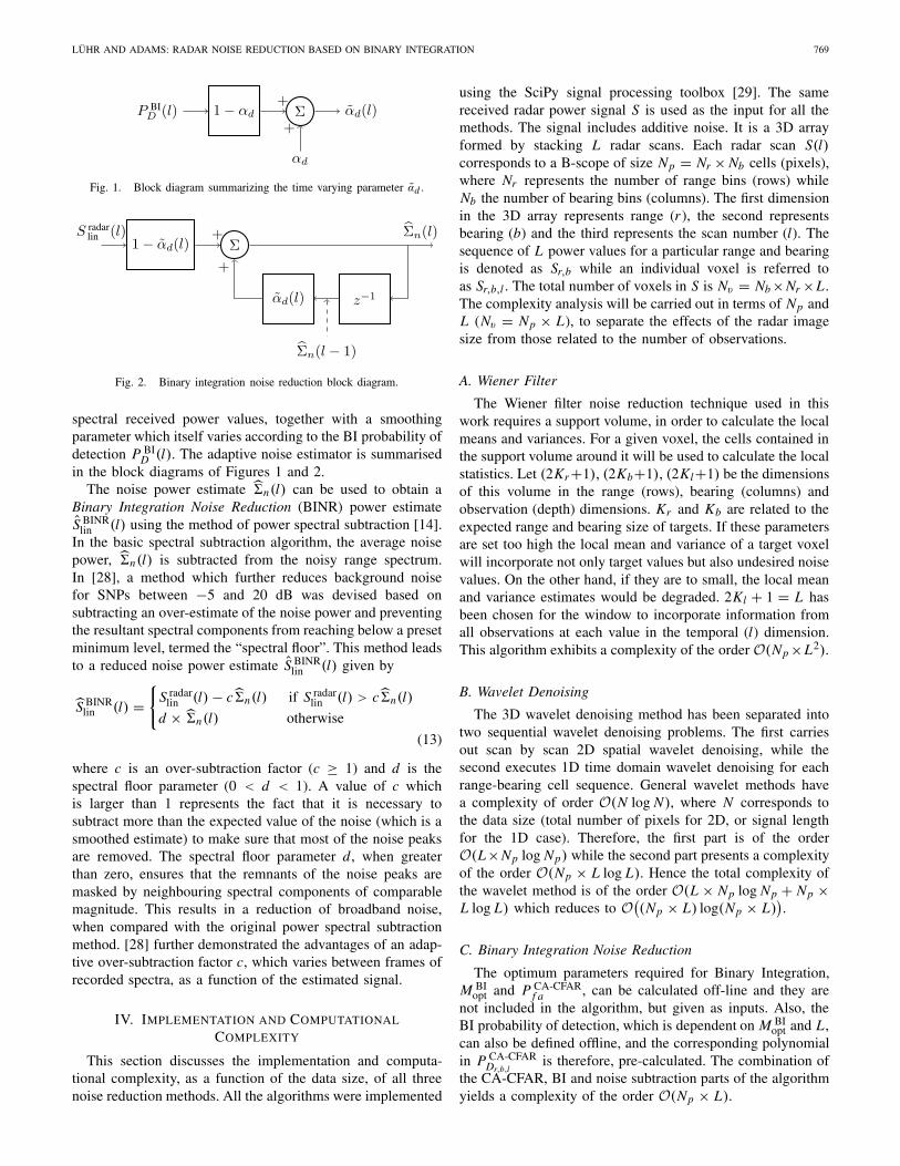
Fig. 1. Block diagram summarizing the time varying parameter αd .

Fig. 2. Binary integration noise reduction block diagram.

spectral received power values, together with a smoothingparameter which itself varies according to the BI probability ofdetection P BI

D (l). The adaptive noise estimator is summarisedin the block diagrams of Figures 1 and 2.

The noise power estimate �n(l) can be used to obtain aBinary Integration Noise Reduction (BINR) power estimateS BINR

lin (l) using the method of power spectral subtraction [14].In the basic spectral subtraction algorithm, the average noisepower, �n(l) is subtracted from the noisy range spectrum.In [28], a method which further reduces background noisefor SNPs between −5 and 20 dB was devised based onsubtracting an over-estimate of the noise power and preventingthe resultant spectral components from reaching below a presetminimum level, termed the “spectral floor”. This method leadsto a reduced noise power estimate S BINR

lin (l) given by

S BINRlin (l) =

{S radar

lin (l) − c�n(l) if S radarlin (l) > c�n(l)

d × �n(l) otherwise

(13)

where c is an over-subtraction factor (c ≥ 1) and d is thespectral floor parameter (0 < d < 1). A value of c whichis larger than 1 represents the fact that it is necessary tosubtract more than the expected value of the noise (which is asmoothed estimate) to make sure that most of the noise peaksare removed. The spectral floor parameter d , when greaterthan zero, ensures that the remnants of the noise peaks aremasked by neighbouring spectral components of comparablemagnitude. This results in a reduction of broadband noise,when compared with the original power spectral subtractionmethod. [28] further demonstrated the advantages of an adap-tive over-subtraction factor c, which varies between frames ofrecorded spectra, as a function of the estimated signal.

IV. IMPLEMENTATION AND COMPUTATIONAL

COMPLEXITY

This section discusses the implementation and computa-tional complexity, as a function of the data size, of all threenoise reduction methods. All the algorithms were implemented

using the SciPy signal processing toolbox [29]. The samereceived radar power signal S is used as the input for all themethods. The signal includes additive noise. It is a 3D arrayformed by stacking L radar scans. Each radar scan S(l)corresponds to a B-scope of size Np = Nr × Nb cells (pixels),where Nr represents the number of range bins (rows) whileNb the number of bearing bins (columns). The first dimensionin the 3D array represents range (r ), the second representsbearing (b) and the third represents the scan number (l). Thesequence of L power values for a particular range and bearingis denoted as Sr,b while an individual voxel is referred toas Sr,b,l . The total number of voxels in S is Nv = Nb ×Nr ×L.The complexity analysis will be carried out in terms of Np andL (Nv = Np × L), to separate the effects of the radar imagesize from those related to the number of observations.

A. Wiener Filter

The Wiener filter noise reduction technique used in thiswork requires a support volume, in order to calculate the localmeans and variances. For a given voxel, the cells contained inthe support volume around it will be used to calculate the localstatistics. Let (2Kr +1), (2Kb+1), (2Kl+1) be the dimensionsof this volume in the range (rows), bearing (columns) andobservation (depth) dimensions. Kr and Kb are related to theexpected range and bearing size of targets. If these parametersare set too high the local mean and variance of a target voxelwill incorporate not only target values but also undesired noisevalues. On the other hand, if they are to small, the local meanand variance estimates would be degraded. 2Kl + 1 = L hasbeen chosen for the window to incorporate information fromall observations at each value in the temporal (l) dimension.This algorithm exhibits a complexity of the order O(Np ×L2).

B. Wavelet Denoising

The 3D wavelet denoising method has been separated intotwo sequential wavelet denoising problems. The first carriesout scan by scan 2D spatial wavelet denoising, while thesecond executes 1D time domain wavelet denoising for eachrange-bearing cell sequence. General wavelet methods havea complexity of order O(N log N), where N corresponds tothe data size (total number of pixels for 2D, or signal lengthfor the 1D case). Therefore, the first part is of the orderO(L×Np log Np) while the second part presents a complexityof the order O(Np × L log L). Hence the total complexity ofthe wavelet method is of the order O(L × Np log Np + Np ×L log L) which reduces to O(

(Np × L) log(Np × L)).

C. Binary Integration Noise Reduction

The optimum parameters required for Binary Integration,M BI

opt and P CA-CFARf a , can be calculated off-line and they are

not included in the algorithm, but given as inputs. Also, theBI probability of detection, which is dependent on M BI

opt and L,can also be defined offline, and the corresponding polynomialin P CA-CFAR

Dr,b,lis therefore, pre-calculated. The combination of

the CA-CFAR, BI and noise subtraction parts of the algorithmyields a complexity of the order O(Np × L).


Fig. 3. Elapsed computational time measurement.

In summary, with respect to observations L, the Wiener filteralgorithm has the highest complexity (quadratic), followed bythe linearithmic3 complexity of the Wavelet approach, whilethe binary integration noise reduction’s linear complexitymakes it the least complex. On the other hand, the Wienerfilter and the binary integration noise reduction are the leastcomplex (linear time) with respect to the data size Nv .

V. RESULTS

All of the noise reduction methods have been tested withreal data obtained in a local park environment and with anopen SAR image data set. The results show reduced noiseradar power in PPI representation, as well as, the average noiselevel versus observation number. In order to demonstrate theusefulness of each reduced noise data set, the CFAR detectionmethod is finally applied to each set. CA-CFAR is used in thepark data set due to its compliance to the detector requirementsas described in Section II, while OS-CFAR is used in theSAR data set, which has been proven to be more effectivewith this kind of data [34]. The reduced noise CFAR outputis then compared to the CFAR detector’s result on the originalnoisy data. The computational times of the algorithms are alsocompared.

A. Computational Time

The computational time used by the different algorithms,plotted against observation number L, is shown in Figure 3.The results are consistent with the analysis presented insection IV. The Wiener filter’s complexity grows approxi-mately quadratically with L, while the wavelet exhibits lin-earithmic complexity. A linear time complexity is achievedby the BINR method.

B. Experimental Data

An experimental radar data set, captured4 in a public parkin Santiago, is used to test the noise reduction schemes.

3A linearithmic function is of the form n log n. An algorithm with a timecomplexity of the order O(n log n) is said to run in linearithmic time.

4using an Acumine 94 GHz, scanning radar [31].

Fig. 4. Park environment where radar data was captured (obtained fromGoogle Earth).

TABLE I

OPTIMAL MBI PARAMETER FOR DIFFERENT

NUMBER OF OBSERVATIONS L

1) Noise Reduction: Noise values in real radar data donot conform to perfect Gaussian or exponential distributions,as assumed by the noise reduction methods, which impairstheir performance. An analysis of the noise reduction methodsconsidering the park environment now follows. Although themethods were applied to the B-Scope radar data (range vs.bearing), the results are shown in plan position indicator (PPI)form for clearer visualisation. The test environment is shownin Figure 4. The area corresponds to a main paved trackapproximately 65 m wide. On the sides of the track there arelamp posts and some trees. There are also fences and concretewalls. The radar was located on the track.

The CA-CFAR window size was 9 bins in the bearingdirection and 7 bins in the range direction. The guard cellswindow size was 5 in the bearing dimension and 3 bins inthe range direction. These parameters were found suitable, inpreliminary experiments, for detecting the lamp posts and treessurrounding the radar, by considering the power spread thesefeatures produce in the acquired data.

The BI false alarm rate used was 1 × 10−6. The optimalMBI has been previously obtained for different L values.Some of the values are listed in Table I. The results presentedcorrespond to L = 20 observations. For the noise subtractionalgorithm, the chosen parameters were αd = 0.9, c = 50.0and d = 0.1. A high αd ensures that the previous value ofthe noise estimate has more weight than the new observationwhich is desirable given the high noise levels present in radardata. Parameter c, controlling over-subtraction, was selectedby testing different values between 10 and 100. Similarly,the spectral floor parameter d was tested for different valuesbetween 0.05 to 0.5, with the chosen value yielding goodresults in the reduction of the broadband noise.


Fig. 5. Raw power and reduced noise power PPI plots of the park area. (a) PPI showing noisy input data from the park environment. (b) PPI showingWiener filtered data from the park environment. (c) PPI showing Wavelet denoised data from the park environment. (d) PPI showing BINR data from thepark environment.

The Wiener support region was 3 bins in the range andbearing direction, which is the expected power spread of thetargets of interest.

In the case of the spatial (2D) wavelet denoising, theDaubechies 3 wavelet function was used, while the Haarwavelet was selected for the 1D (temporal) dimension.

The noisy raw radar input data from the park is presented inFigure 5a. The ground truth location of lamp posts and treesare marked with green circles and a cross in their centre.

Wiener filtering (Figure 5b) exhibits a smoother noise back-ground but the main objects identified in the scene are blurredby the filter, thus losing localisation detail. Wavelet denoising(Figure 5c), is able to preserve the location and edges of tar-gets. It does, however, produce several negative values in noiseonly sections, which are truncated to a small value to allowvisualisation. Nevertheless, the average noise level is reduced.Finally, the BINR method in Figure 5d shows its ability toretain details as well as to reduce the noise level. It can, how-ever, be observed that some of the maximum power peaks havebeen reduced in magnitude (e.g. tree at (−49.1 m, 48.6 m);with a raw power value of 86.02 dB and a BINR power valueof 82.73 dB). This is due to the fact that at some observationl those particular targets were not detected, therefore theirpower values were considered noise and thus subtracted fromthem. Note that wavelet denoising (Figure 5c) reduces some

Fig. 6. Noise mean values and variances from a noise only area.

noise-only areas to very low values. However, the noisebackground is not homogeneous, therefore, the sharp edgesbetween noise areas near the average noise level and thosegreatly reduced by the wavelet method can yield several falsedetections as will be shown, after applying the CA-CFARdetector.

Figure 6 shows mean noise power values from each method,in an area which is known to contain no targets. The BINR


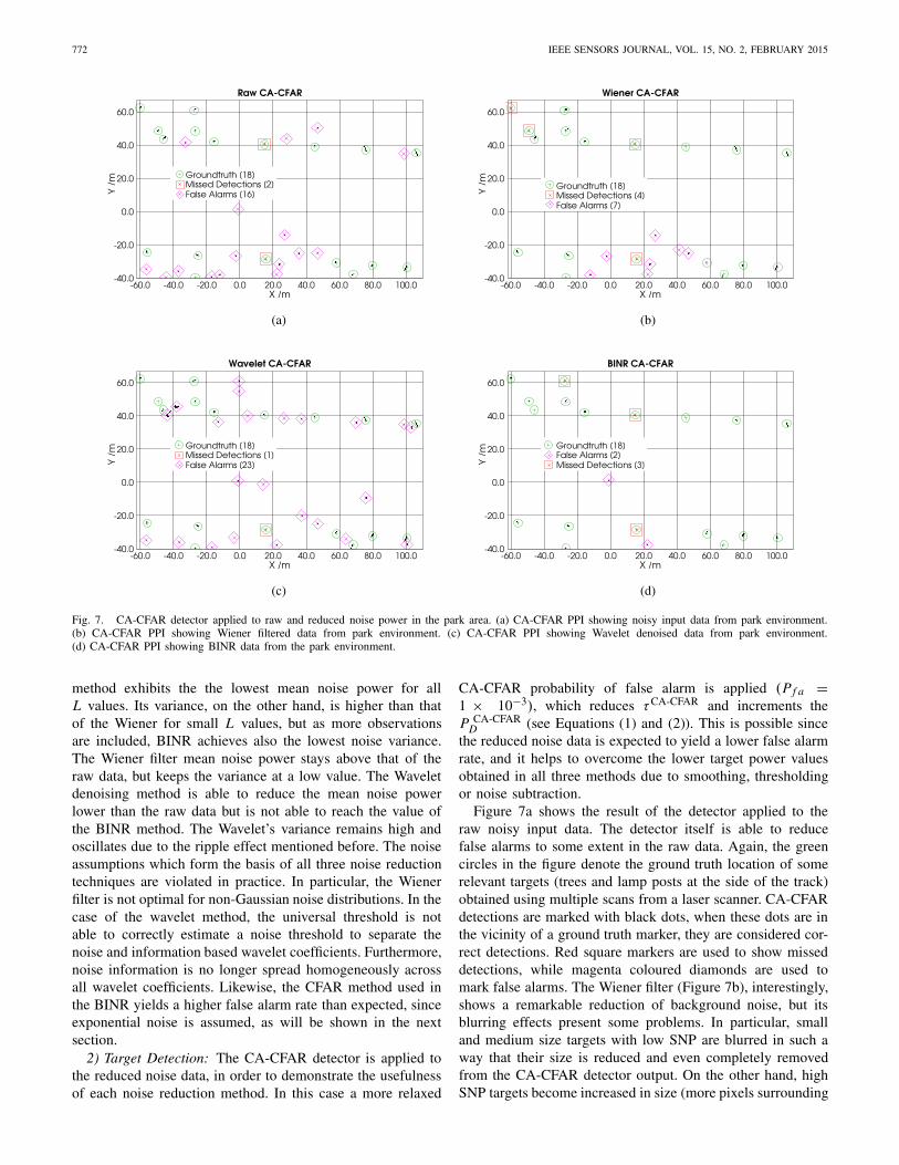
Fig. 7. CA-CFAR detector applied to raw and reduced noise power in the park area. (a) CA-CFAR PPI showing noisy input data from park environment.(b) CA-CFAR PPI showing Wiener filtered data from park environment. (c) CA-CFAR PPI showing Wavelet denoised data from park environment.(d) CA-CFAR PPI showing BINR data from the park environment.

method exhibits the the lowest mean noise power for allL values. Its variance, on the other hand, is higher than thatof the Wiener for small L values, but as more observationsare included, BINR achieves also the lowest noise variance.The Wiener filter mean noise power stays above that of theraw data, but keeps the variance at a low value. The Waveletdenoising method is able to reduce the mean noise powerlower than the raw data but is not able to reach the value ofthe BINR method. The Wavelet’s variance remains high andoscillates due to the ripple effect mentioned before. The noiseassumptions which form the basis of all three noise reductiontechniques are violated in practice. In particular, the Wienerfilter is not optimal for non-Gaussian noise distributions. In thecase of the wavelet method, the universal threshold is notable to correctly estimate a noise threshold to separate thenoise and information based wavelet coefficients. Furthermore,noise information is no longer spread homogeneously acrossall wavelet coefficients. Likewise, the CFAR method used inthe BINR yields a higher false alarm rate than expected, sinceexponential noise is assumed, as will be shown in the nextsection.

2) Target Detection: The CA-CFAR detector is applied tothe reduced noise data, in order to demonstrate the usefulnessof each noise reduction method. In this case a more relaxed

CA-CFAR probability of false alarm is applied (Pf a =1 × 10−3), which reduces τCA-CFAR and increments theP CA-CFAR

D (see Equations (1) and (2)). This is possible sincethe reduced noise data is expected to yield a lower false alarmrate, and it helps to overcome the lower target power valuesobtained in all three methods due to smoothing, thresholdingor noise subtraction.

Figure 7a shows the result of the detector applied to theraw noisy input data. The detector itself is able to reducefalse alarms to some extent in the raw data. Again, the greencircles in the figure denote the ground truth location of somerelevant targets (trees and lamp posts at the side of the track)obtained using multiple scans from a laser scanner. CA-CFARdetections are marked with black dots, when these dots are inthe vicinity of a ground truth marker, they are considered cor-rect detections. Red square markers are used to show misseddetections, while magenta coloured diamonds are used tomark false alarms. The Wiener filter (Figure 7b), interestingly,shows a remarkable reduction of background noise, but itsblurring effects present some problems. In particular, smalland medium size targets with low SNP are blurred in such away that their size is reduced and even completely removedfrom the CA-CFAR detector output. On the other hand, highSNP targets become increased in size (more pixels surrounding


TABLE II

A POSTERIORI DETECTION AND FALSE ALARM RATES

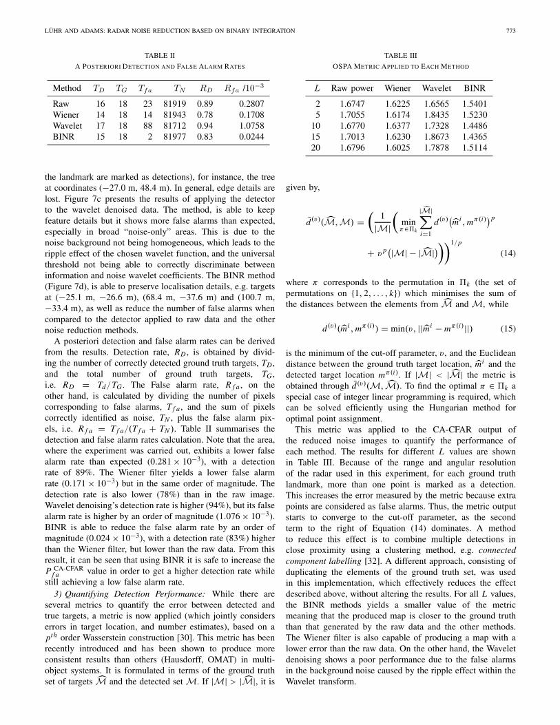
the landmark are marked as detections), for instance, the treeat coordinates (−27.0 m, 48.4 m). In general, edge details arelost. Figure 7c presents the results of applying the detectorto the wavelet denoised data. The method, is able to keepfeature details but it shows more false alarms than expected,especially in broad “noise-only” areas. This is due to thenoise background not being homogeneous, which leads to theripple effect of the chosen wavelet function, and the universalthreshold not being able to correctly discriminate betweeninformation and noise wavelet coefficients. The BINR method(Figure 7d), is able to preserve localisation details, e.g. targetsat (−25.1 m, −26.6 m), (68.4 m, −37.6 m) and (100.7 m,−33.4 m), as well as reduce the number of false alarms whencompared to the detector applied to raw data and the othernoise reduction methods.

A posteriori detection and false alarm rates can be derivedfrom the results. Detection rate, RD , is obtained by divid-ing the number of correctly detected ground truth targets, TD ,and the total number of ground truth targets, TG ,i.e. RD = Td/TG . The False alarm rate, R f a , on theother hand, is calculated by dividing the number of pixelscorresponding to false alarms, T f a , and the sum of pixelscorrectly identified as noise, TN , plus the false alarm pix-els, i.e. R f a = T f a/(T f a + TN ). Table II summarises thedetection and false alarm rates calculation. Note that the area,where the experiment was carried out, exhibits a lower falsealarm rate than expected (0.281 × 10−3), with a detectionrate of 89%. The Wiener filter yields a lower false alarmrate (0.171 × 10−3) but in the same order of magnitude. Thedetection rate is also lower (78%) than in the raw image.Wavelet denoising’s detection rate is higher (94%), but its falsealarm rate is higher by an order of magnitude (1.076 × 10−3).BINR is able to reduce the false alarm rate by an order ofmagnitude (0.024 × 10−3), with a detection rate (83%) higherthan the Wiener filter, but lower than the raw data. From thisresult, it can be seen that using BINR it is safe to increase theP CA-CFAR

f a value in order to get a higher detection rate whilestill achieving a low false alarm rate.

3) Quantifying Detection Performance: While there areseveral metrics to quantify the error between detected andtrue targets, a metric is now applied (which jointly considerserrors in target location, and number estimates), based on apth order Wasserstein construction [30]. This metric has beenrecently introduced and has been shown to produce moreconsistent results than others (Hausdorff, OMAT) in multi-object systems. It is formulated in terms of the ground truthset of targets M and the detected set M. If |M| > |M|, it is

TABLE III

OSPA METRIC APPLIED TO EACH METHOD

given by,

d(v)(M,M) =(

1

|M|(

minπ∈�k

|M|∑i=1

d(v)(mi , mπ(i))p

+ v p(|M| − |M|)))1/p

(14)

where π corresponds to the permutation in �k (the set ofpermutations on {1, 2, . . . , k}) which minimises the sum ofthe distances between the elements from M and M, while

d(v)(mi , mπ(i)) = min(v, ||mi − mπ(i)||) (15)

is the minimum of the cut-off parameter, v, and the Euclideandistance between the ground truth target location, mi and thedetected target location mπ(i). If |M| < |M| the metric isobtained through d(v)(M,M). To find the optimal π ∈ �k aspecial case of integer linear programming is required, whichcan be solved efficiently using the Hungarian method foroptimal point assignment.

This metric was applied to the CA-CFAR output ofthe reduced noise images to quantify the performance ofeach method. The results for different L values are shownin Table III. Because of the range and angular resolutionof the radar used in this experiment, for each ground truthlandmark, more than one point is marked as a detection.This increases the error measured by the metric because extrapoints are considered as false alarms. Thus, the metric outputstarts to converge to the cut-off parameter, as the secondterm to the right of Equation (14) dominates. A methodto reduce this effect is to combine multiple detections inclose proximity using a clustering method, e.g. connectedcomponent labelling [32]. A different approach, consisting ofduplicating the elements of the ground truth set, was usedin this implementation, which effectively reduces the effectdescribed above, without altering the results. For all L values,the BINR methods yields a smaller value of the metricmeaning that the produced map is closer to the ground truththan that generated by the raw data and the other methods.The Wiener filter is also capable of producing a map with alower error than the raw data. On the other hand, the Waveletdenoising shows a poor performance due to the false alarmsin the background noise caused by the ripple effect within theWavelet transform.


Fig. 8. Yahoo Satellite view (left) and Raw SAR image of the area (right).

C. UAVSAR Data Set

Detection and noise reduction methods in radar are notonly used in classical A-Scopes, B-Scopes and PPIs, theycan also be used in other forms of radar data such as SARimages [20], [33].

SAR images, being constructed in a fundamentally differentway than the classical radar images, are also affected by noisein a different way. In SAR images, noise and clutter areusually modelled by a Weibull or K distribution. Also, theeffect of multiplicative speckle noise in SAR images is higherthan in other forms of radar data. Under these conditions, theOrdered Statistics (OS) CFAR detection method has proven tobe effective when applied to SAR images [34].

In this section the results of using the BINR method on a setof SAR images obtained from the NASA Jet Propulsion Lab(JPL)’s Uninhabited Aerial Vehicle SAR (UAVSAR) mission5

are presented.The images correspond to a location near Sacramento, CA,

which covers an area of crop fields with isolated buildings inthe north-most part (top) of the image and a suburban areawith high density housing in the south-most part (bottom).Figure 8 (left) shows a Yahoo Satellite image of the area,with its corresponding SAR image (right). The area is 1.6 kmin the horizontal (east-west) direction and 2.88 km in thevertical (north-south) direction. These SAR images representbackscatterred radar power, polarised in the HH, HV and VVcomponents. The magnitude of each component is encoded inthe image’s red, green and blue channels, respectively.

BINR based on the OS-CFAR detector has been used tofirst reduce the noise in a series of multiple (L = 6, MBI = 3)observations of the same area. Then the OS-CFAR detectoris applied to the reduced noise data to detect buildings.The OS-CFAR window size was 7 bins in the x and ycoordinates, while the guard cells window size was 3 bins

5UAVSAR data courtesy NASA/JPL-Caltech. http://uavsar.jpl.nasa.gov/

TABLE IV

MEAN NOISE POWER AND VARIANCE IN NOISE ONLY AREA IN dB

in both directions. The threshold’s constant parameter chosenwas τOS-CFAR = 4.16707, this value is obtained by solvingEq. (6) using the OS-CFAR window size and the desired valuefor POS-CFAR

f a . Finally, the noise subtraction parameters usedwere αd = 0.9, c = 50.0 and d = 0.1.

The parameters for Wavelet denoising and Wiener filteringwere the same as those used in the experimental data setpresented in Section V-B.

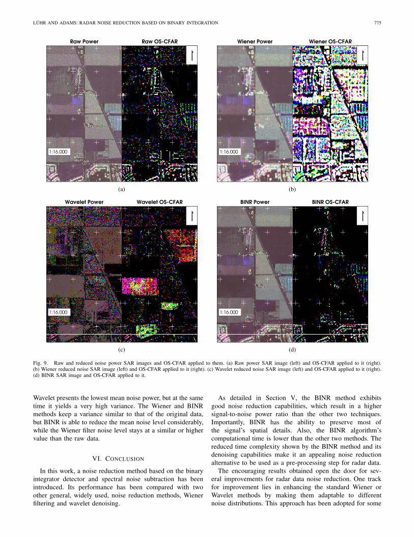
All three polarisation components have been processed.Buildings, in general, reflect radar waves similarly in allpolarisations while vegetation and other terrain consideredto be clutter in this case, usually exhibit different back-scatter intensity at the different polarisations. The raw power(left) and the output of the OS-CFAR detector are shownin Figure 9a. In the OS-CFAR image, the red, green andblue pixels corresponds to detections in the HH, HV and VVpolarisations, respectively. Cyan, magenta and yellow pixelsrepresent detections in the respective combinations of twopolarisations, while white pixels represent detections in allthree polarisations. Buildings appear in the OS-CFAR imagewith white pixels (detections in all polarisations), while parksand crop fields present detections in single polarisations or nodetection at all.

The Wiener filtering results are presented in Figure 9b. Thereduced noise image appears blurred, as expected from theWiener filter, and the OS-CFAR detector is unable to detectbuildings from the crop fields.

The wavelet denoising output is shown in Figure 9c. Thepower image shows darker colours meaning that the averagenoise power has been reduced, but several areas present a highvariance, particularly in the crop fields. The OS-CFAR outputconfirms this, and the detector is unable to detect buildingstructures.

Figure 9d corresponds to BINR output. It can be observedthat the areas corresponding to crop fields appear smoothedwhen compared to the raw image. It can also be observedthat the number of detections in single polarisations, mostlylocated in areas corresponding to crop fields, is reduced in theBINR image. On the other hand, most pixels correspondingto building like structures are preserved.

In this data set it is not possible to apply the OSPA metricas the real ground truth is unavailable. An analysis on thenoise statistics in an area with no targets, as was carried outin the park data set, quantifies the performance of the noisereduction methods. Table IV shows the mean noise power andvariance per polarisation channel. It can be observed that the


Fig. 9. Raw and reduced noise power SAR images and OS-CFAR applied to them. (a) Raw power SAR image (left) and OS-CFAR applied to it (right).(b) Wiener reduced noise SAR image (left) and OS-CFAR applied to it (right). (c) Wavelet reduced noise SAR image (left) and OS-CFAR applied to it (right).(d) BINR SAR image and OS-CFAR applied to it.

Wavelet presents the lowest mean noise power, but at the sametime it yields a very high variance. The Wiener and BINRmethods keep a variance similar to that of the original data,but BINR is able to reduce the mean noise level considerably,while the Wiener filter noise level stays at a similar or highervalue than the raw data.

VI. CONCLUSION

In this work, a noise reduction method based on the binaryintegrator detector and spectral noise subtraction has beenintroduced. Its performance has been compared with twoother general, widely used, noise reduction methods, Wienerfiltering and wavelet denoising.

As detailed in Section V, the BINR method exhibitsgood noise reduction capabilities, which result in a highersignal-to-noise power ratio than the other two techniques.Importantly, BINR has the ability to preserve most ofthe signal’s spatial details. Also, the BINR algorithm’scomputational time is lower than the other two methods. Thereduced time complexity shown by the BINR method and itsdenoising capabilities make it an appealing noise reductionalternative to be used as a pre-processing step for radar data.

The encouraging results obtained open the door for sev-eral improvements for radar data noise reduction. One trackfor improvement lies in enhancing the standard Wiener orWavelet methods by making them adaptable to differentnoise distributions. This approach has been adopted for some


wavelet denoising applications in which different thresh-old functions are derived for some non-Gaussian noisedistributions [12], [35], [36]. This can then be the basis forthe integration of 2 or more of the methods. This has beencarried out for Wiener and Wavelet filtering in the workof Jin et al. [13]. This work exploited the advantages ofboth methods simultaneously, but even though the theoreticalimprovement in peak-to-peak SNR was expected to be 3dB,only 0.5dB was achieved. Also the time complexity ofJin et al’s method corresponds to the combination of boththe Wiener and wavelet methods. In particular, it wouldbe interesting to evaluate optimised combinations of theWiener filter and BINR, Wavelet denoising and BINR, andthe Wiener-Wavelet and the BINR method, in terms of theircomputational complexities. These combinations would beexpected to yield the advantages of the individual methods,for instance, the smooth background noise presented by theWiener filter, the reduction in the mean noise power valueprovided by the BINR method, and the faithful representa-tion of the original signal achieved when applying waveletdenoising.

ACKNOWLEDGMENT

The authors would like to thank NASA/JPL-Caltech for allUAVSAR data.

REFERENCES

[1] J. C. Brailean, R. P. Kleihorst, S. Efstratiadis, A. K. Katsaggelos, andR. L. Lagendijk, “Noise reduction filters for dynamic image sequences:A review,” Proc. IEEE, vol. 83, no. 9, pp. 1272–1292, Sep. 1995.

[2] N. Wiener, Extrapolation, Interpolation, and Smoothing of StationaryTime Series. Cambridge, MA, USA: MIT Press, 1964.

[3] B. Widrow et al., “Adaptive noise cancelling: Principles and applica-tions,” Proc. IEEE, vol. 63, no. 12, pp. 1692–1716, Dec. 1975.

[4] M. Martin-Fernandez, C. Alberola-Lopez, J. Ruiz-Alzola, andC.-F. Westin, “Sequential anisotropic Wiener filtering applied to 3DMRI data,” Magn. Reson. Imag., vol. 25, no. 2, pp. 278–292, 2007.[Online]. Available: http://www.sciencedirect.com/science/article/pii/S0730725X06002852

[5] I. N. Daliakopoulos and I. K. Tsanis, “A weather radar data process-ing module for storm analysis,” J. Hydroinformat., vol. 14, no. 2,pp. 332–344, 2012.

[6] D. Donoho, “De-noising by soft-thresholding,” IEEE Trans. Inf. Theory,vol. 41, no. 3, pp. 613–627, May 1995.

[7] D. L. Donoho and J. M. Johnstone, “Ideal spatial adaptation by waveletshrinkage,” Biometrika, vol. 81, no. 3, pp. 425–455, 1994. [Online].Available: http://biomet.oxfordjournals.org/content/81/3/425.abstract

[8] D. L. Donoho and I. M. Johnstone, “Threshold selection for waveletshrinkage of noisy data,” in Proc. 16th Annu. Int. Conf. IEEE Eng. Med.Biol. Soc. Eng. Adv., New Opportunities Biomed. Eng., vol. 1. no. 12,Nov. 1994, pp. A24–A25.

[9] C. Burrus, R. Gopinath, and H. Guo, Introduction to Wavelets andWavelet Transforms: A Primer, vol. 23. Upper Saddle River, NJ, USA:Prentice-Hall, 1998.

[10] M.-Y. Chen and J.-J. Chao, “Radar image denoising by recursivethresholding,” in Proc. Int. Conf. Image Process., vol. 1. Sep. 1996,pp. 395–398.

[11] O. A. M. Aly, A. S. Omar, and A. Z. Elsherbeni, “Detectionand localization of RF radar pulses in noise environments usingwavelet packet transform and higher order statistics,” Prog. Elec-tromagn. Res., vol. 58, pp. 301–317, 2006. [Online]. Available:http://jpier.org/pier/pier.php?paper=0507024

[12] Y. Chen and C. Han, “Adaptive wavelet thresholding for image denois-ing and compression,” Electron. Lett., vol. 41, no. 10, pp. 586–587,May 2005.

[13] F. Jin, P. Fieguth, L. Winger, and E. Jernigan, “Adaptive wiener filteringof noisy images and image sequences,” in Proc. Int. Conf. ImageProcess. (ICIP), vol. 3. Sep. 2003, pp. III-349–III-352.

[14] S. Boll, “Suppression of acoustic noise in speech using spectral sub-traction,” IEEE Trans. Acoust., Speech, Signal Process., vol. 27, no. 2,pp. 113–120, Apr. 1979.

[15] M. I. Skolnik, Ed., “Automatic detection, tracking, and sensor integra-tion,” in Radar Handbook, 3rd ed. New York, NY, USA: McGraw-Hill,2008.

[16] P. P. Gandhi and S. A. Kassam, “Optimality of the cell averagingCFAR detector,” IEEE Trans. Inf. Theory, vol. 40, no. 4, pp. 1226–1228,Jul. 1994.

[17] A. Foessel, J. Bares, and W. R. L. Whittaker, “Three-dimensionalmap building with MMW radar,” in Proc. 3rd Int. Conf. FieldService Robot., Helsinki, Finland, Jun. 2001. [Online]. Available:http://www.ri.cmu.edu/publication_view.html?pub_id=3758&menu_code=0307

[18] D. Langer, “An integrated MMW radar system for outdoor navigation,”in Proc. IEEE Int. Conf. Robot. Autom., Minneapolis, MN, USA,Apr. 1996, pp. 417–422.

[19] M. Barkat, Signal Detection and Estimation, ser. Artech House RadarLibrary. Norwood, MA, USA: Artech House, 2005. [Online]. Available:http://books.google.com/books?id=Le5SAAAAMAAJ

[20] G. Gao, L. Liu, L. Zhao, G. Shi, and G. Kuang, “An adaptive andfast CFAR algorithm based on automatic censoring for target detectionin high-resolution SAR images,” IEEE Trans. Geosci. Remote Sens.,vol. 47, no. 6, pp. 1685–1697, Jun. 2009.

[21] H. Rohling, “Radar CFAR thresholding in clutter and multiple targetsituations,” IEEE Trans. Aerosp. Electron. Syst., vol. AES-19, no. 4,pp. 608–621, Jul. 1983.

[22] N. Wiener, Extrapolation, Interpolation, and Smoothing of Station-ary Time Series: With Engineering Applications (Technology PressBooks in Science and Engineering). Cambridge, MA, USA: MIT Press,1949.

[23] A. Kolmogorov, Stationary Sequences in Hilbert Space. Chicago, IL,USA: John Crerar Library, 1978.

[24] J.-S. Lee, “Digital image enhancement and noise filtering by use of localstatistics,” IEEE Trans. Pattern Anal. Mach. Intell., vol. PAMI-2, no. 2,pp. 165–168, Mar. 1980.

[25] D. L. Donoho and I. M. Johnstone, “Ideal denoising in an orthonormalbasis chosen from a library of bases,” Comptes Rendus Acad. Sci., Ser. I,vol. 319, no. 12, pp. 1317–1322, 1994.

[26] G. Luo and D. Zhang, “Wavelet denoising,” in Advances in WaveletTheory and Their Applications in Engineering, Physics and Technol-ogy. Rijeka, Croatia: InTech, 2012, pp. 59–80. [Online]. Available:http://www.intechopen.com/

[27] I. Cohen and B. Berdugo, “Noise estimation by minima controlled recur-sive averaging for robust speech enhancement,” IEEE Signal Process.Lett., vol. 9, no. 1, pp. 12–15, Jan. 2002.

[28] M. Berouti, R. Schwartz, and J. Makhoul, “Enhancement of speechcorrupted by acoustic noise,” in Proc. IEEE Int. Conf. Acoust., Speech,Signal Process. (ICASSP), vol. 4. Apr. 1979, pp. 208–211.

[29] E. Jones, T. Oliphant, and P. Peterson. (2001). SciPy: Open SourceScientific Tools for Python. [Online]. Available: http://www.scipy.org/

[30] S. Kuttikkad and R. Chellappa, “Non-Gaussian CFAR techniques fortarget detection in high resolution SAR images,” in Proc. IEEE Int.Conf. Image Process. (ICIP), vol. 1. Nov. 1994, pp. 910–914.

[31] E. Widzyk-Capehart, G. Brooker, S. Scheding, R. Hennessy, A. Maclean,and C. Lobsey, “Application of millimetre wave radar sensor to envi-ronment mapping in surface mining,” in Proc. 9th Int. Conf. Control,Autom., Robot. Vis. (ICARCV), Dec. 2006, pp. 1–6.

[32] D. Schuhmacher, B.-T. Vo, and B.-N. Vo, “A consistent metric forperformance evaluation of multi-object filters,” IEEE Trans. SignalProcess., vol. 56, no. 8, pp. 3447–3457, Aug. 2008.

[33] L. Shapiro and G. Sockman, Computer Vision. Englewood Cliffs, NJ,USA: Prentice-Hall, 2002, ch. 3.

[34] M. di Bisceglie and C. Galdi, “CFAR detection of extended objects inhigh-resolution SAR images,” in Proc. IEEE Int. Geosci. Remote Sens.Symp. (IGARSS), vol. 6. Jul. 2001, pp. 2674–2676.

[35] S. Zhong and V. Cherkassky, “Image denoising using wavelet thresh-olding and model selection,” in Proc. Int. Conf. Image Process., vol. 3.2000, pp. 262–265.

[36] A. Antoniadis, D. Leporini, and J.-C. Pesquet, “Wavelet thresholdingfor some classes of non–Gaussian noise,” Statist. Neerlandica, vol. 56,no. 4, pp. 434–453, 2002.


Daniel Lühr (S’99–M’04) was born in Santiago,Chile, in 1978. He received the Lic.Sci. and Diplomadegrees in electrical engineering from the Universityof Chile, Santiago, Chile, in 2003 and 2004, respec-tively.

He was a Research Associate and No-Fee Con-sultant with the Submillimeter Receiver Laboratory,Harvard-Smithsonian Center for Astrophysics, Cam-bridge, MA, USA, from 2004 to 2006. From 2007to 2009, he was an Adjunct Professor with theUniversidad Austral de Chile, Valdivia, Chile. From

2009 to 2013, he was a Consultant with the Chilean Ministry of Energy. He iscurrently with the Department of Electrical Engineering, University of Chile.He has expertise in digital systems, system integration, medical devices, androbotics. His current research interests include robotics and its applications.

Martin Adams (SM’08) received the degree inengineering science from the University of Oxford,Oxford, U.K., in 1988, and the Ph.D. degreefrom the Robotics Research Group, Universityof Oxford, in 1992. He is currently a Profes-sor of Electrical Engineering with the Depart-ment of Electrical Engineering, University of Chile,Santiago, Chile. He is also a Principle Investigatorwith the industrially sponsored Advanced MiningTechnology Centre, University of Chile. After hisPh.D., he continued his research in autonomous

robot navigation as a Project Leader and part-time Lecturer with the Instituteof Robotics, Swiss Federal Institute of Technology, Zurich, Switzerland. Hewas a Guest Professor and taught control theory in St. Gallen, Switzerland,from 1994 to 1995. From 1996 to 2000, he served as a Senior ResearchScientist in Robotics and Control, in the field of semiconductor assemblyautomation, with the European Semiconductor Equipment Centre, Cham,Switzerland. From 2000 to 2010, he was an Associate Professor with theSchool of Electrical and Electronic Engineering, Nanyang Technological Uni-versity, Singapore. His research work focuses on autonomous robot navigation,sensing, and multiobject estimation, and has authored many technical papers inthese fields. He has been a Principle Investigator and leader of many roboticsprojects, coordinating researchers from local industries and local and overseasuniversities, and has served as an Associate Editor of various journal andconference editorial boards.

766 ieee sensors journal, vol. 15, no. 2, february 2015

Documents