7758 ch05 130-161 12/5/03 4:30 pm page 130 5 · pdf file7758_ch05_130-161 12/5/03 4:30 pm page...
TRANSCRIPT

Why might a firm decide to storeits products in a warehouse
rather than offer them forsale?
What’s the meaning of theold expression “Too manycooks spoil the broth”?
Can a firm shut downwithout going out ofbusiness?
Why do movie theatershave so many screens?
C o n s i d e r
P O I N T Y O U R B R O W S E R
econxtra.swlearning.com
Supply
The Supply Curve 5.1Shifts of the Supply Curve 5.2
Production and Cost 5.3
5©
Get
ty I
mag
es/P
hoto
Dis
c
7758_CH05_130-161 12/5/03 4:30 PM Page 130

ObjectivesUnderstand the law ofsupply.
Describe the elasticityof supply, and explainhow it is measured.
Key Terms supply
law of supply
supply curve
elasticity of supply
OverviewJust as consumer behavior shapes thedemand curve, producer behavior shapesthe supply curve. When studying demand,you should think like a consumer, or ademander. When studying supply, however,you must think like a producer, or a sup-plier. You may feel more natural as a con-sumer—after all, you are a consumer. Butyou know more about producers than youmay realize. You have been around them allyour life—Wal-Mart, Sony, Blockbuster,Exxon, McDonald’s, Microsoft, Kinko’s, Ford,Home Depot, Sears, Gap, and hundredsmore. You will draw on this knowledge todevelop an understanding of supply and thesupply curve.
The Supply Curve5.1
Pay Phones Don’t Pay Anymore
Where will Clark Kent change into his Superman outfit now that it’s getting harderand harder to find a phone booth? Pay phones are being eliminated from all the famil-iar spots—shopping centers, gasoline stations, restaurants, and street corners. Itseems they’re just not profitable anymore. In the mid-1990s, there were as many as2.7 million pay phones across the country. That number is down to about 1.9 millionnow, and dropping. For the most part, they have been replaced by wireless cellphones. The few small companies that collect the monies and service pay phonesare leaving the business. These companies have found that even with an increasedprice of 50 cents a call, the majority of pay phones operate at a loss when factoringin the costs of cleaning, maintaining, and repairing them. For the time being, payphones continue to be supplied and maintained in the low-income areas of cities.Many people who live in these areas can’t afford to own any type of phone, and sopay phones are still profitable there.
Think About It
What, if anything, can suppliers of pay phones do to save their industry?
[ In the News ]
131
7758_CH05_130-161 12/5/03 4:30 PM Page 131

Law of SupplyWith demand, the assumption is thatconsumers try to maximize utility, agoal that motivates their behavior. Withsupply, the assumption is that producerstry to maximize profit. Profit is the goalthat motivates the behavior of suppliers.
Role of ProfitIn trying to earn a profit, firms trans-form productive resources into prod-ucts. Profit equals total revenue minustotal cost. Total revenue is the totalsales, or total dollars, received fromconsumers for the day, week, or year.Total cost includes the cost of allresources used by a firm in producinggoods or services, including the entrepreneur’s opportunity cost.
Profit � Total revenue � Total Cost
When a firm breaks even, total revenuejust covers total cost. Over time, totalrevenue must cover total cost for thefirm to survive. If total revenue fallsshort of total cost year after year,entrepreneurs will find more attractiveuses for resources, and the firm willfail.
Each year, millions of new firmsenter the U.S. marketplace and nearlyas many leave. The firms must decidewhat goods and services to produceand what resources to employ. Firmsmust make plans while facing uncer-tainty about consumer demand,resource availability, and the intentionsof other firms in the market. The lureof profit is so strong that entrepreneursare always eager to pursue theirdreams.
SupplyJust as demand is a relation betweenprice and quantity demanded, supply isa relation between price and quantitysupplied. Supply indicates how muchof a good producers are willing and ableto offer for sale per period at each pos-sible price, other things constant. Thelaw of supply says that the quantitysupplied is usually directly related to itsprice, other things constant. Thus, thelower the price, the smaller the quantitysupplied. The higher the price, thegreater the quantity supplied.
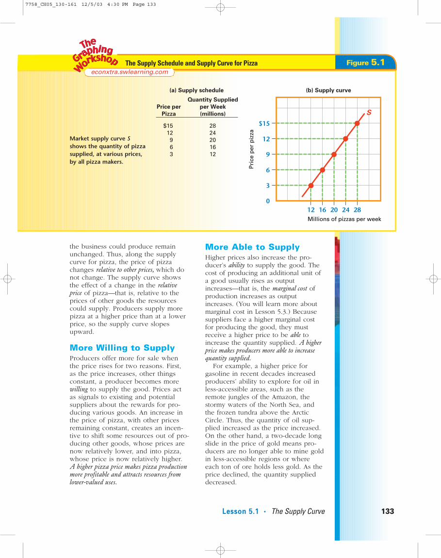
Figure 5.1 presents the market supplyschedule and market supply curve Sfor pizza. Both show the quantities of12-inch pizzas supplied per week atvarious possible prices by the manypizza makers in the market. As you cansee, price and quantity supplied aredirectly (or positively) related, otherthings constant. The supply curveshows, for example, that at a price of$6 per pizza, the quantity supplied is16 million per week. At a price of $9per pizza, the quantity suppliedincreases to 20 million.
Like the demand curve, the supplycurve represents a particular period oftime. It shows quantity supplied perperiod. For any supply curve, it isassumed that the prices of other goods
132 CHAPTER 5 Supply
supplyA relation showingthe quantities of agood producers arewilling and able tosell at various pricesduring a givenperiod, other thingsconstant
law of supplyThe quantity of agood suppliedduring a given timeperiod is usuallydirectly related to itsprice, other thingsconstant
supply curve A curve or lineshowing the quanti-ties of a particulargood supplied atvarious prices duringa given time period,other things constant
Entrepreneurs take the risks of organizingproductive resources to make goodsand services. A restaurant venture isan especially risky business that usesthe productive resources of peopleand food to prepare and servemeals to customers. The profit incentive leads restaurant entrepre-neurs to accept the risks of businessfailure.
©G
etty
Im
ages
/Pho
toD
isc
Profit and EntrepreneurMai
n Idea
Mai
n Idea
7758_CH05_130-161 12/5/03 4:30 PM Page 132
the business could produce remainunchanged. Thus, along the supplycurve for pizza, the price of pizzachanges relative to other prices, which donot change. The supply curve showsthe effect of a change in the relativeprice of pizza—that is, relative to theprices of other goods the resourcescould supply. Producers supply morepizza at a higher price than at a lowerprice, so the supply curve slopesupward.
More Willing to SupplyProducers offer more for sale whenthe price rises for two reasons. First,as the price increases, other thingsconstant, a producer becomes morewilling to supply the good. Prices actas signals to existing and potentialsuppliers about the rewards for pro-ducing various goods. An increase inthe price of pizza, with other pricesremaining constant, creates an incen-tive to shift some resources out of pro-ducing other goods, whose prices arenow relatively lower, and into pizza,whose price is now relatively higher.A higher pizza price makes pizza productionmore profitable and attracts resources fromlower-valued uses.
More Able to SupplyHigher prices also increase the pro-ducer’s ability to supply the good. Thecost of producing an additional unit ofa good usually rises as outputincreases—that is, the marginal cost ofproduction increases as outputincreases. (You will learn more aboutmarginal cost in Lesson 5.3.) Becausesuppliers face a higher marginal costfor producing the good, they mustreceive a higher price to be able toincrease the quantity supplied. A higherprice makes producers more able to increasequantity supplied.
For example, a higher price forgasoline in recent decades increasedproducers’ ability to explore for oil inless-accessible areas, such as theremote jungles of the Amazon, thestormy waters of the North Sea, andthe frozen tundra above the ArcticCircle. Thus, the quantity of oil sup-plied increased as the price increased.On the other hand, a two-decade longslide in the price of gold means pro-ducers are no longer able to mine goldin less-accessible regions or whereeach ton of ore holds less gold. As theprice declined, the quantity supplieddecreased.
Lesson 5.1 The Supply Curve 133
Market supply curve Sshows the quantity of pizzasupplied, at various prices,by all pizza makers.
econxtra.swlearning.comFigure 5.1The Supply Schedule and Supply Curve for Pizza
(a) Supply schedule
Quantity Supplied
per Week
(millions)
Price per
Pizza
$1512963
2824201612
(b) Supply curve
12 16 20 24 280
3
6
9
12
$15
Millions of pizzas per week
Pri
ce p
er p
izza
S
7758_CH05_130-161 12/5/03 4:30 PM Page 133

In short, a higher price makes pro-ducers more willing and better able toincrease quantity supplied. Suppliers aremore willing because production of thehigher-priced good now is more prof-itable than the alternative uses of theresources involved. Suppliers are betterable because the higher price allowsthem to cover the higher marginal costthat typically results from increasingproduction.
Supply Versus QuantitySuppliedAs with demand, economists distinguishbetween supply and quantity supplied.Supply is the entire relation between theprice and quantity supplied, as reflectedby the supply schedule or supply curve.Quantity supplied refers to a particularamount offered for sale at a particularprice, as reflected by a point on a givensupply curve. Thus, it is the quantity sup-plied that increases with a higher price,not supply. The term supply by itselfrefers to the entire supply schedule orsupply curve.
Individual Supply andMarket SupplyEconomists also distinguish betweenindividual supply (the supply of an indi-vidual producer) and market supply (the
supply of all producers in the market).The market supply curve shows the totalquantity supplied by all producers at variousprices.
In most markets, there are many sup-pliers, sometimes thousands. Assume forsimplicity, however, that there are justtwo suppliers in the market for pizza:Pizza Palace and Pizza Castle. Figure 5.2shows how the supply curves for twoproducers in the market are addedtogether to yield the market supplycurve. Individual supply curves aresummed across to get a market supplycurve.
For example, at a price of $9, PizzaPalace supplies 400 pizzas per weekand Pizza Castle supplies 300. Thus,the quantity supplied in the market for pizza at a price of $9 is 700. At a price of $12, Pizza Palace supplies 500 and Pizza Castle supplies 400, for a market supply of 900 pizzas per week. The market supply curve in panel (c) of Figure 5.2 shows the horizontal sums of the indi-vidual supply curves in panels (a) and (b).
The market supply curve is simply the hori-zontal sum of the individual supply curves forall producers in the market. Unless other-wise noted, when this book talks aboutsupply, you can take that to meanmarket supply.
134 CHAPTER 5 Supply
The market supply curve is the horizontal sum of each individual supply curve.
Figure 5.2Summing Individual Supply Curves to Find the Market Supply Curve
9
$12
(a) Pizza Palace (b) Pizza Castle (c) Market Supply
Sm Sp Sm + Sp = S
400 5000
Pizzas per week Pizzas per week Pizzas per week
Pri
ce
400300
9
$12
700 900
9
$12
7758_CH05_130-161 12/5/03 4:30 PM Page 134

Elasticity ofSupplyPrices are signals to both sides of themarket about the relative scarcity ofproducts. High prices discourage con-sumption but encourage production.The elasticity of demand measures howresponsive consumers are to a pricechange. Likewise, the elasticity ofsupply measures how responsive pro-ducers are to a price change.
MeasurementThe elasticity of supply is calculated inthe same way as the elasticity ofdemand. The elasticity of supplyequals the percentage change in quan-tity supplied divided by the percentagechange in price.
Elasticity of supply =
Suppose the price increases. Becausea higher price usually results in anincreased quantity supplied, the per-centage change in price and the per-centage change in quantity suppliedmove in the same direction. So, theprice elasticity of supply usually is apositive number.
Figure 5.3 depicts the typical upward-sloping supply curve presented earlier.As you can see, if the price of pizzaincreases from $9 to $12, the quantitysupplied increases from 20 million to 24 million. What’s the elasticity ofsupply? The percentage change in quan-tity supplied is the change in quantitysupplied—4 million—divided by 20million. So quantity supplied increasesby 20 percent. The percentage changein price is the change in price—$3—divided by $9, which is 33 percent.
The elasticity of supply is, therefore,the percentage increase in quantity
Percentage change inquantity supplied
Percentagechange in price
Lesson 5.1 The Supply Curve 135
If the price increases from $9 to $12, the quantity of pizzasupplied increases from 20 million to 24 million per week.
econxtra.swlearning.comFigure 5.3The Supply of Pizza
20 24 280
9
12
Millions of pizzas per week
Pri
ce p
er p
izza
$15
6
3
12 16
S
Explain the law of supply in yourown words.
C H E C K P O I N T
elasticity ofsupplyA measure of theresponsiveness ofquantity supplied toa price change; thepercentage changein quantity supplieddivided by the percentage changein price
7758_CH05_130-161 12/5/03 4:30 PM Page 135

supplied—20 percent—divided by thepercentage increase in price—33percent—which equals 0.6.
Categories of SupplyElasticityThe terminology for supply elasticity isthe same as for demand elasticity. Ifsupply elasticity exceeds 1.0, supply is
elastic. If it equals 1.0, supply is unitelastic. If supply is less than 1.0, it isinelastic. Because 0.6 is less than 1.0, thesupply of pizza is inelastic when theprice increases from $9 to $12. Notethat elasticity usually varies along asupply curve.
Determinants of SupplyElasticityThe elasticity of supply indicates howresponsive producers are to a changein price. Their responsiveness dependson how costly it is to alter output whenthe price changes. If the marginal costof supplying additional units risessharply as output expands, then ahigher price will generate little increasein quantity supplied, so supply willtend to be inelastic. However, if themarginal cost rises slowly as outputexpands, the profit lure of a higherprice will prompt a relatively largeboost in output. In this case, supplywill be more elastic.
One important determinant of supplyelasticity is the length of the adjustmentperiod under consideration. Just asdemand becomes more elastic overtime as consumers adjust to pricechanges, supply also becomes moreelastic over time as producers adjust toprice changes. The longer the timeperiod under consideration, the moreeasily producers can adjust. Forexample, a higher oil price will promptsuppliers to pump more from existingwells in the short run. However, in thelong run, suppliers can explore formore oil.
Figure 5.4 demonstrates how thesupply of gasoline becomes moreelastic over time, with a differentsupply curve for each of three periods.Sw is the supply curve when the periodof adjustment is a week. As you cansee, a higher gasoline price will notprompt much of a response in quantitysupplied because firms have little timeto adjust. This supply curve is inelasticif the price increases from $1.00 to$1.25 per gallon.
Sm is the supply curve when theadjustment period under consideration isa month. Firms have a greater ability to
136 CHAPTER 5 Supply
Mongolian Goats and the Price of Cashmere Sweaters
Think there’s a connection? Cashmere comes from the hairof cashmere goats, the majority of which (some 10 million)are raised primarily in Mongolia and northern China.Although that’s a lot of goats, each one yields only about21/2 pounds of fleece per shearing. That 21/2 pounds, inturn, produces only about 5 ounces of usable cashmerefiber after the labor-intensive job of cleaning and de-hairing.Consequently, the price of the warmer, softer cashmereusually is far higher than its competitor, wool. In past years,Mongolia’s exports of this unique product have grown dra-matically and, up until 2003, totaled around 2,000 tons withits internal usage of the product between 1,600 and 2,000tons annually. Unfortunately for the Mongolian producers,the price of cashmere currently is down from a high ofalmost $20 per pound in 2002 to $9 a pound. This pricedecline has caused the Mongolian herdsmen to stockpilemore than 3,000 tons of the material.
Think Critically
In the short run (over the next few months), is Mongolia’ssupply of cashmere elastic or inelastic along the supply curveat the price of $9 per pound? Mongolia barely raises enoughfood for its people, much less its animals, and more than amillion of the goats recently have starved to death. In view ofthis, would you consider the longer-term response to the $9price to be elastic or inelastic? Explain your answer.
7758_CH05_130-161 12/5/03 4:30 PM Page 136

vary output in a month than they do in aweek. Thus, supply is more elastic whenthe adjustment period is a month thanwhen it’s a week. Supply is even moreelastic when the adjustment period is ayear, as is shown by Sy. A given priceincrease in gasoline prompts a greaterquantity supplied as the adjustmentperiod lengthens. Research confirms thepositive link between the elasticity ofsupply and the length of the adjustmentperiod. The elasticity of supply is typicallygreater the longer the period of adjustment.
The ease of increasing quantity sup-plied in response to a higher pricediffers across industries. The long runwill be longer for producers of electric-ity and timber (where expansion maytake years) than for window washingand hot-dog vending (where expansionmay take only days).
Lesson 5.1 The Supply Curve 137
The supply curve one week after a priceincrease, Sw, is less elastic, at a given price,than the curve one month later, Sm, whichis less elastic than the curve one year later,Sy. Given a price increase from $1.00 to$1.25, quantity supplied per day increasesto 110 million gallons after one week, to140 gallons after one month, and to 200million gallons after one year.
Figure 5.4Market Supply Becomes More Elastic Over Time
Working in small groups, think offive industries other than thosegiven as examples in this textbook.For each industry, describe theproduct or services sold, as wellas the means of distribution, suchas retail stores, online, or whole-sale. Rank these industries inorder of the time the industryneeds to adjust to a price change.Give a ranking of 1 to industriesthat would require the leastamount of time to adjust fully to aprice change and a 5 to those thatwould require the most time.Provide an explanation for each ofyour rankings. Discuss yourgroup’s rankings in class.
TEAM WORK
Sw Sm
Sy
140 2000
1.00
Millions of gallons per day
Pri
ce p
er g
allo
n
$1.25
100 110
What does the elasticity of supplymeasure, and what factors influ-ence its numerical value?
C H E C K P O I N T
7758_CH05_130-161 12/5/03 4:30 PM Page 137
Key Concepts1. In what ways are the motives of a pizza restaurant owner different from the
motives of customers who buy the restaurant’s pizza?
2. Why should the quantity of winter jackets supplied increase when there is anincrease in the price of these jackets?
3. There are three restaurants that open at 7:00 A.M. to serve breakfast in a smallcommunity. Each one charges $4.00 for two eggs, bacon, toast and a cup ofcoffee. Together they sell 220 breakfasts on an average weekday morning.What is the individual and market supply in this situation?
4. When the market price of kitchen chairs increases by 10 percent, producers ofthese chairs increase the quantity supplied by 20 percent. Is supply elastic, unitelastic, or inelastic? Explain how you know your answer is correct. What is themeasure of elasticity in this situation?
5. Why is the price elasticity of supply likely to be greater for wooden bowls thanfor natural pearls?
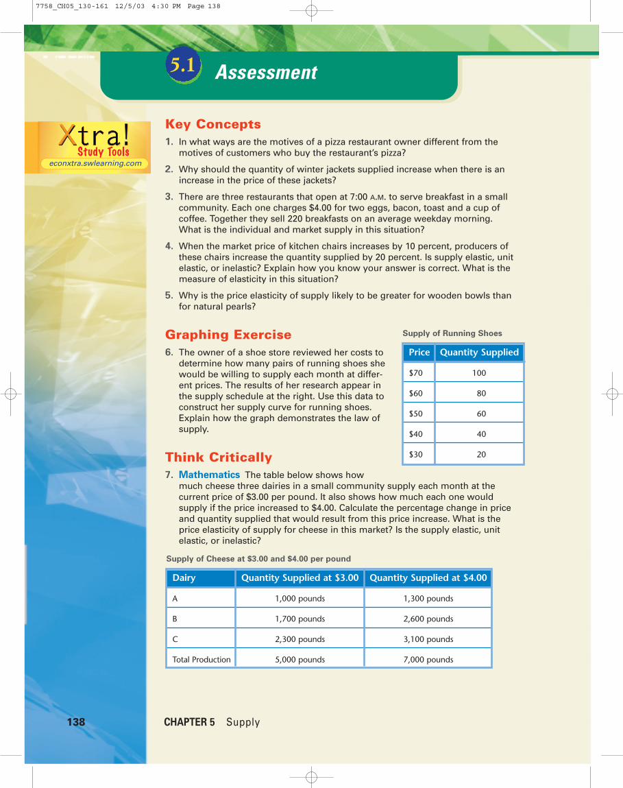
Graphing Exercise6. The owner of a shoe store reviewed her costs to
determine how many pairs of running shoes shewould be willing to supply each month at differ-ent prices. The results of her research appear inthe supply schedule at the right. Use this data toconstruct her supply curve for running shoes.Explain how the graph demonstrates the law ofsupply.
Think Critically7. Mathematics The table below shows how
much cheese three dairies in a small community supply each month at thecurrent price of $3.00 per pound. It also shows how much each one wouldsupply if the price increased to $4.00. Calculate the percentage change in priceand quantity supplied that would result from this price increase. What is theprice elasticity of supply for cheese in this market? Is the supply elastic, unitelastic, or inelastic?
138 CHAPTER 5 Supply
Supply of Running Shoes
Price Quantity Supplied
$70 100
$60 80
$50 60
$40 40
$30 20
Supply of Cheese at $3.00 and $4.00 per pound
Dairy Quantity Supplied at $3.00 Quantity Supplied at $4.00
A 1,000 pounds 1,300 pounds
B 1,700 pounds 2,600 pounds
C 2,300 pounds 3,100 pounds
Total Production 5,000 pounds 7,000 pounds
Assessment5.1
econxtra.swlearning.com
7758_CH05_130-161 12/5/03 4:30 PM Page 138

Understand Cause and EffectIn economics, as in most other fieldsof study, things don’t “just happen.”There is a logical reason, or a cause,for almost every economic event. One goal of studying economicevents that have taken place in thepast is to learn about their causes sowe can predict what will happenwhen similar events take place in thefuture. Consider each of the followingevents from American history andtheir results. What can you learn that could help you better understandfuture economic events?
In 1892, workers at the CarnegieSteel Plant in Homestead, Penn-sylvania, went on strike, closing downthis factory. This reduced the supply ofsteel and may have contributed toworkers at other factories that usedsteel being laid off.
In 1903, the Wright brothers werecredited with having made the firstpowered flight. This led to a newmode of transportation that millions ofAmericans now use each year. With afew exceptions, the supply curve of airtransportation has steadily moved tothe right over time.
In 1929, the stock market crash con-tributed to the failure of thousands ofU.S. businesses and the onset of theGreat Depression of the 1930s. The
supply of many products fell duringthe early years of the Great Depression.
In 1938, the Fair Labor StandardsAct was passed that established the40-hour workweek. This caused somebusinesses to hire additional workersto avoid paying workers overtimewages and may have increased theircost of production. If this was true, thesupply curve for these firms’ productswould have shifted to the left.
Apply Your Skill1. At the beginning of 2003, President
George W. Bush suggested reduc-ing taxes for businesses that pur-chased new machinery or hiredadditional workers. Describe theeffect that this suggested policywas intended to cause. How wouldit affect the supply of many prod-ucts in the U.S. economy?
2. In 2003, farmers in central Californiawere told that they were takingmore than their share of water fromthe Colorado River. They wereordered to plan to reduce theamount of water they took for irriga-tion. Nearly a third of the lettuceand many other vegetables grownin the United States are produced incentral California. If this ruling wereenforced, what might happen to thesupply of vegetables American con-sumers could buy?
Sharpen Your Life Skills
Lesson 5.1 The Supply Curve 139
7758_CH05_130-161 12/5/03 4:30 PM Page 139

5.2Shifts of the Supply Curve
Conflict vs. Clean Diamonds
In 2003, President George W. Bush signed the Clean Diamond Trade Act. The Actshould decrease markedly the importation and sale of diamonds from several nationswhere brutal regimes control their production. The Act institutionalizes the KimberleyProcess Certification Scheme. This scheme or plan is intended to insure that diamondsentering the United States are certified as not being “conflict diamonds.” These are dia-monds that have been mined and sold to finance decades-long wars and atrocities inAfrica and have reportedly financed al-Qaeda as well. More than 50 countries, both pro-ducing and importing nations, have agreed to participate in the plan. In addition, thediamond industry has agreed to establish a system of warranties under which dealerspurchase stones only from sellers who can prove the merchandise’s legitimacy.
Think About It
What effect(s) do you think this Act will have on the supply curve of diamonds in theUnited States?
[ In the News ]
ObjectivesIdentify the determi-nants of supply, andexplain how a changein each will affect thesupply curve.
Contrast a movementalong the supplycurve with a shift ofthe supply curve.
Key Terms movement along a
supply curve
shift of a supply curve
OverviewThe supply curve illustrates the relationbetween the price of a good and the quan-tity supplied, other things constant. Assumedconstant along a supply curve are the deter-minants of supply other than the good’sprice. There are five such determinants ofsupply. A change in one of these determi-nants of supply causes a shift of the supplycurve. This contrasts with a change in price,other things constant, that causes a move-ment along a supply curve.
140
7758_CH05_130-161 12/5/03 4:30 PM Page 140

Determinantsof SupplyBecause each firm’s supply curve isbased on the cost of production andprofit opportunities in the market, any-thing that affects production costs andprofit opportunities helps shape thesupply curve. Following are the fivedeterminants of market supply otherthan the price of the good:
1. The cost of resources used to makethe good
2. The price of other goods theseresources could make
3. The technology used to make the good
4. Producer expectations
5. The number of sellers in the market
Changes in the Price of ResourcesAny change in the costs of resources usedto make a good will affect the supply ofthe good. For example, suppose the priceof mozzarella cheese falls. This reducesthe cost of making pizza. Producers are
therefore more willing and able to supplypizza at each price, as reflected by arightward shift of the supply curve from Sto S ′ in Figure 5.5. After the shift, thequantity supplied increases at each pricelevel. For example, at a price of $12, thequantity supplied is higher from 24million to 28 million pizzas a week, asshown by the movement from point g topoint h. In short, an increase in supply—thatis, a rightward shift of the supply curve—meansthat producers are more willing and able to supplymore pizzas at each price.
What if there is an increase in theprice of a resource used to make pizza?This means that at every level of output,the cost of supplying pizza increases.An increase in the price of a resourcewill reduce supply, meaning a leftwardshift of the supply curve. For example,if the wage of pizza workers increases,the higher labor cost would increase thecost of making pizza.
Higher production costs decreasesupply, so pizza supply shifts leftward,as from S to S ′′ in Figure 5.6. After thedecrease in supply, producers offer lessfor sale at each price. For example, at aprice of $12 per pizza, the quantity sup-plied falls from 24 million to 20 million
Lesson 5.2 Shifts of the Supply Curve 141
An increase in the supply of pizza is reflected bya rightward shift of the supply curve, from S toS′. After the increase in supply, the quantity ofpizza supplied at a price of $12 increases from24 million pizzas (point g) to 28 million pizzas(point h).
econxtra.swlearning.comFigure 5.5An Increase in the Supply of Pizza
S ′S
12 16 20 24 280
3
6
9
12
$15
Millions of pizzas per week
Pri
ce p
er p
izza
gh
7758_CH05_130-161 12/9/03 6:12 PM Page 141

per week. This is shown in Figure 5.6 bythe movement from point g to point i.
Changes in the Prices ofOther GoodsNearly all resources have alternativeuses. The labor, building, machinery,ingredients, and knowledge needed tomake pizza could produce other prod-ucts, such as bread sticks, rolls, andother baked goods.
A change in the price of anothergood these resources could makeaffects the opportunity cost of makingpizza. For example, if the price of rollsfalls, the opportunity cost of makingpizza declines. These resources are notas profitable in their best alternativeuse, which is making rolls. So pizzaproduction becomes relatively moreattractive. As resources shift frombaking rolls to making pizza, the supplyof pizza increases, or shifts to the right,as shown in Figure 5.5.
On the other hand, if the price of rollsincreases, so does the opportunity costof making pizza. Some pizza makersmay bake more rolls and less pizza, sothe supply of pizza decreases, or shifts tothe left, as in Figure 5.6. A change in theprice of another good these resources
could produce affects the profit opportu-nities available to producers.
Changes in TechnologyThe state of technology represents theeconomy’s stock of knowledge abouthow to combine resources efficiently.Discoveries in chemistry, biology, elec-tronics, and many other fields havecreated new products, improved existingproducts, and lowered the cost of pro-duction. For example, the first micro-processor, the Intel 4004, could executeabout 400 computations per secondwhen it hit the market in 1971. Today astandard PC often can handle more than2 billion computations per second, or 5million times what the 1971 Intel 4004could handle. Technological change—inthis case, faster computers—lowers thecost of producing goods whose produc-tion involves computers, from automobilemanufacturing to document processing.
Along a given market supply curve,technological know-how about how thisgood can be manufactured is assumedto remain unchanged. If a more efficienttechnology is discovered, the cost ofproduction will fall, making this marketmore profitable. Improvements in tech-nology make firms more willing and
142 CHAPTER 5 Supply
A decrease in the supply of pizza is reflected by aleftward shift of the supply curve, from S to S ′′.After the decrease in supply, the quantity of pizzasupplied at a price of $12 decreases from 24 millionpizzas (point g) to 20 million pizzas (point i).
Figure 5.6A Decrease in the Supply of Pizza
S ′′ S
i
12 16 20 24 280
3
6
9
12
$15
Millions of pizzas per week
Pri
ce p
er p
izza
g
7758_CH05_130-161 12/9/03 6:12 PM Page 142

able to supply the good at each price.Consequently, supply will increase, asreflected by a rightward shift of thesupply curve. For example, suppose anew high-tech oven bakes pizza in halfthe time. Such a breakthrough wouldshift the supply curve rightward, asfrom S to S ′ in Figure 5.5, so that moreis supplied at each possible price.
Changes in ProducerExpectationsProducers transform resources intogoods they hope can be sold for aprofit. Any change that affects producerexpectations about profitability canaffect market supply. For example, ifpizza prices are expected to increase inthe future, some pizza makers mayexpand production capacity now. Thiswould shift the supply of pizza right-ward, as shown in Figure 5.5.
Some goods can be stored easily. Forexample, crude oil can be left in theground and grain can be stored in asilo. Expecting higher prices in thefuture might prompt some producers ofthese goods to reduce their currentsupply while awaiting the higher price.This would shift the supply curve to theleft, as shown in Figure 5.6. Thus, anexpectation of higher prices in the
future could either increase or decreasecurrent supply, depending on the good.
Changes in the Numberof Sellers in the MarketGeneral changes in the market environ-ment also can affect the number ofsellers in the market. For example, gov-ernment regulations may influencemarket supply. As a case in point, fordecades government strictly regulated theprices and entry of new firms in a varietyof industries including airlines, trucking,and telecommunications. During thatperiod, the number of firms in the marketwas artificially limited by these govern-ment restrictions. When these restrictionswere eliminated, more firms enteredthese markets, increasing supply.
Any government action that affects amarket’s profitability, such as a changein business taxes, could shift the supplycurve. Lower business taxes willincrease supply and higher businesstaxes will reduce supply.
The increase in the number of firms isnot simply a response to a price change.Along a given market supply curve, thereusually are fewer suppliers at lowerprices than higher prices. Higher pricesattract producers and increase the quan-tity supplied along the supply curve.
MovementsAlong a SupplyCurve VersusShifts of aSupply CurveNote again the distinction between amovement along a supply curve and a shift ofa supply curve. A change in price, otherthings constant, causes a movementalong a supply curve from one price-
Lesson 5.2 Shifts of the Supply Curve 143
Businesses generally payincome taxes to local, state,and the federal govern-ment. Contact your localgovernment’s bureau of tax-ation. Find out the currenttax rate for businesses. Alsofind the rate for the pastfive years. Has an increaseor decrease in the tax rateaffected supply in yourarea? Write a paragraph toexplain your findings.
What are the five determinants ofsupply, and how do changes ineach affect the supply of a good?
C H E C K P O I N T
movementalong a supplycurveChange in quantitysupplied resultingfrom a change in theprice of the good,other things constant
7758_CH05_130-161 12/5/03 4:30 PM Page 143

quantity combination to another. Achange in one of the determinants ofsupply other than the price causes ashift of a supply curve, changingsupply. A shift of the supply curvemeans a change in the quantity sup-plied at each price.
A change in price, other things con-stant, changes quantity supplied along a
given supply curve. A change in a deter-minant of supply other than the price ofthe good—such as the prices ofresources used to make the good, tech-nology used to make the good, the priceof other goods these resources couldproduce, producer expectations, and thenumber of firms in the market—shifts theentire supply curve to the right or left.
144 CHAPTER 5 Supply
Read the E-conomics feature, below, about the useof credit-card technology at fast-food restaurants.McDonald’s Corporation is working with eMacDigital in developing its new point-of-sale (POS) soft-ware system. To learn more about the relationshipbetween McDonald’s and eMac, access two pressreleases through econxtra.swlearning.com. Why didMcDonald’s sell its ownership interest in eMac?How is this consistent with McDonald’s focus onspecialization and division of labor? What determi-nant of supply does the POS system represent?
econxtra.swlearning.com
Faster Fast Food Pay for your BigMac with a credit card? McDonald’s has beentesting the system and says customers soon willbe able to pay for their burgers and fries withcredit cards. In a world of charging everything onplastic cards, fast-food chains have been slow toget with the program. But customers want to beable to put just about everything they buy on acredit card. According to a market research firm, ifcredit-card use really takes hold, service at fast-food outlets will become even faster. The lines willmove more quickly because the latest high-speedtechnologies and fiber-optic networks are makingcredit-card transactions even faster than paying
with cash. Current technologies enable a cus-tomer to call out an order at the drive-through, orat the counter, and then swipe a credit card andhave it approved in less than 5 seconds. On theother hand, cash transactions take an average of 8to 10 seconds. With widespread use of creditcards, fast-food outlets will be able to supply morehungry customers in the same amount of time.
Think CriticallyWill the use of credit-card technology at fast-food restaurants be likely to cause a movementalong the supply curve or a shift of the supplyfor fast food? Explain your answer.
Explain the difference between amovement along a supply curveand a shift of a supply curve.
C H E C K P O I N T
shift of asupply curveIncrease or decreasein supply resultingfrom a change in oneof the determinantsof supply other thanthe price of the good
7758_CH05_130-161 12/9/03 6:12 PM Page 144
Key Concepts1. One year a farmer grows corn on his 200 acres of land. He sells his corn in
September for $3.00 per bushel. Early the next spring he notices that the priceof soybeans has gone up 50 percent while the price of corn has remained thesame. What will probably happen to his supply curve for corn? Explain youranswer.
2. The Apex Plastics Corp. finds a new way to produce plastic outdoor furniturefrom recycled milk bottles at very low cost. What will happen to the supplycurve for plastic furniture? Explain your answer.
3. A big storm destroys most of the sugarcane crop in Louisiana. Most peopleexpect this to cause a large increase in the price of sugar in the next fewmonths. What will happen to the supply curve for sugar?
4. The cost of crude oil increases by 25 percent. Crude oil is the basic raw materialused to produce plastic. What will this do to the supply curve for plastic toys?
5. How might an increase in the minimum wage shift both the demand curve andsupply curve for pizza?
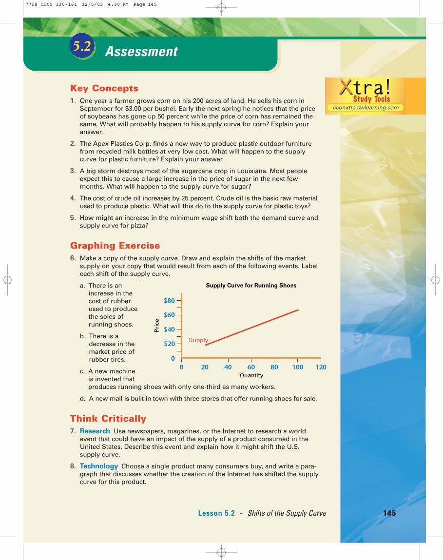
Graphing Exercise6. Make a copy of the supply curve. Draw and explain the shifts of the market
supply on your copy that would result from each of the following events. Labeleach shift of the supply curve.
a. There is anincrease in thecost of rubberused to producethe soles ofrunning shoes.
b. There is adecrease in themarket price ofrubber tires.
c. A new machine is invented thatproduces running shoes with only one-third as many workers.
d. A new mall is built in town with three stores that offer running shoes for sale.
Think Critically7. Research Use newspapers, magazines, or the Internet to research a world
event that could have an impact of the supply of a product consumed in theUnited States. Describe this event and explain how it might shift the U.S.supply curve.
8. Technology Choose a single product many consumers buy, and write a para-graph that discusses whether the creation of the Internet has shifted the supplycurve for this product.
Assessment5.2
Lesson 5.2 Shifts of the Supply Curve 145
0 20 40 60 80 100 120
$80
$60
$40
$20
0
Quantity
Supply
Supply Curve for Running Shoes
Pri
ce
econxtra.swlearning.com
7758_CH05_130-161 12/5/03 4:30 PM Page 145

During high school andcollege, John Schnatterearned spending moneyby working part-time innational-chain pizzerias.He noticed somethingmissing from every oneof them: No one was
making a superior-qualitypizza that could be deliv-
ered directly to the customer.He dreamed of one day
opening his own pizza restau-rant, doing everything right.
In 1984, Schnatter graduated from BallState University with a degree in businessadministration and then returned home toJeffersonville, Indiana. There he took thefirst step to introduce the world to his ownsuperior pizza. First he knocked out abroom closet in the rear of his father’sbusiness. Then he sold his beloved 1972Camaro in order to purchase $1,600 worthof used restaurant equipment, includinghis first pizza oven. The first Papa John’srestaurant opened in 1985. Less thantwenty years later 3,000 Papa John’srestaurants operate in 49 states and 12international markets.
Schnatter’s successful business philoso-phy is to focus on one thing and do it betterthan anyone else. He keeps the menusimple and uses only superior-quality ingre-dients. He insists on using fresh (neverfrozen) water-purified traditional dough,vine-ripened fresh-packed tomato sauce,and 100 percent mozzarella cheese.
For four consecutive years, Papa John’swas rated number one in customer satis-faction among all national fast-foodrestaurants in the American Customer
Satisfaction Index. Papa John’s also wasrated number one in product quality in theRestaurants & Institutions’ Choice inChains consumer survey for seven con-secutive years. In 2000, Papa John’sbecome the third-largest pizza company inthe world.
Schnatter established his company head-quarters in Louisville, Kentucky, and is oneof Louisville’s most successful businessleaders. Now in his early forties, this youngentrepreneur is generous with his annualearnings, which exceed $1 million a year.
The pizza market has presented PapaJohn’s with some obstacles. In 2001, theindustry became stagnant, partly becauseof increasingly strong competition fromfrozen grocery pizzas. When things didn’tchange in 2002, Papa John’s largest rivals,Pizza Hut and Dominos, focused on offer-ing deep discounts to customers toincrease sales. Instead of following suit,Schnatter decided his company wouldfocus on product quality and managerretention. He spent between $6 millionand $7 million on these two efforts alone.Schnatter said he believes that “consis-tently getting a better product out thedoor” will result in improved sales, addingthat one way to enhance quality is toreduce staff turnover. The company alsohas begun online ordering.
As Papa John’s founder, Chairman ofthe Board, President, and Chief ExecutiveOfficer, Schnatter continues to be enthusi-astic about making superior-quality pizzasthat can be delivered directly to the cus-tomer. “I love the product, I like thepeople, I love the business. You’ve got tounderstand I’ve been doing this since Iwas 15...It’s all I know.”
movers&shakersmovers&shakersJohn Schnatter Founder, Papa John’s Pizza
SOURCE READINGAnalyze the quotations attributed to JohnSchnatter. From these statements, whatqualities do you think he possesses thatmake him a successful entrepreneur?
ENTREPRENEURS IN ACTIONIn small groups, role-play Papa John’sBoard of Directors, with one student por-
traying Schnatter. The company is facedwith stiff competition from frozen grocerypizzas and deep discounting from its directcompetitors. Discuss the steps manage-ment needs to take in order to keep thecompany growing.
146 CHAPTER 5 Supply
7758_CH05_130-161 12/5/03 4:30 PM Page 146

ObjectivesUnderstand how mar-ginal product variesas a firm employsmore labor in theshort run.
Explain the shape ofthe firm’s marginalcost curve and iden-tify what part of thatis the firm’s supplycurve.
Distinguish betweeneconomies of scaleand diseconomies ofscale in the long run.
OverviewHow much will a firm supply in order tomaximize profit? The answer to this questionrequires a brief introduction to how a firmconverts productive resources into outputs.In general, a profit-maximizing firm willsupply more output to the market as long asthe marginal revenue from each unit soldexceeds its marginal cost.
Production and Cost5.3
At the Local Megaplex
Have you ever wondered why movie theaters seem to be offering moviegoers moreand more screens? Think about it in this way: A theater with one screen needssomeone to sell tickets, someone to sell popcorn, and someone to operate the pro-jector. If another screen is added, the same staff can perform these tasks for bothscreens. Thus, the ticket seller becomes more productive by selling tickets to bothmovies. Also, construction costs per screen are reduced because only one lobby andone set of rest rooms are required. The theater can run bigger, more noticeablenewspaper ads and can spread the cost over more films. From 1990 to 2000, thenumber of screens in the United States grew faster than the number of theaters, sothe average number of screens per theater increased.
Think About It
As you read this section, look for the economic principle this situation illustrates.What do economists call this principle?
[ In the News ]
147
Key Terms short runlong runtotal productmarginal productlaw of diminishing
returnsfixed costvariable costtotal costmarginal costmarginal revenuecompetitive firm’s
supply curveeconomies of scalelong-run average curve
cost
7758_CH05_130-161 12/5/03 4:30 PM Page 147

Production inthe Short RunA firm tries to earn a profit by convert-ing productive resources, or inputs, intogoods and services, or outputs. Considerproduction at a hypothetical movingcompany called Hercules at YourService.
Fixed and VariableResourcesAll producers, like Hercules, use twocategories of resources: fixed and vari-able. Resources that cannot be alteredeasily—the size of the building, forexample—are called fixed resources.Hercules’ fixed resources consist of awarehouse, a moving van, and somemoving equipment. Resources that canbe varied quickly to change output arecalled variable resources. In this example,assume that labor is the only variableresource.
When considering the time requiredto change the quantity of resourcesemployed, economists distinguishbetween the short run and the long run.In the short run, at least one resourceis fixed. In the long run, no resourcesare fixed. Hercules is operating in theshort run because some resources arefixed. In this example, labor is the onlyresource that varies in the short run. Afirm can enter or leave a market in thelong run but not in the short run.
Figure 5.7 relates the amount of laboremployed to the amount of furnishingsmoved. Labor is measured in worker-days, which is one worker for one day,and output is measured in tons of fur-nishings moved per day. The firstcolumn shows the total product perday, measured in tons of furnituremoved. Total product is the total
output of the firm. The secondcolumn shows the number ofworkers required for that totalproduct. The third column shows themarginal product of each worker—
that is, the amount by which the totalproduct changes with each additionalworker, assuming other resourcesremain unchanged.
Increasing Returns Without labor, nothing gets moved, sototal product is zero when no workersare hired. If one worker is hired, thatperson must do all the driving, packing,and moving. A single worker cannoteasily move some of the larger items.Still, one worker manages to move 2tons per day. When a second worker ishired, some division of labor occurs,and two can move the big stuff moreeasily, so production more thandoubles to 5 tons per day. The mar-ginal product of the second worker is 3 tons per day.
Adding a third worker allows for aneven better division of labor, whichcontributes to increased production. Forexample, one worker can specialize inpacking fragile items while the othertwo do the heavy lifting. The totalproduct of three workers is 9 tons perday, 4 tons more than with twoworkers. The firm experiences increasingreturns from labor as each of the firstthree workers is hired, meaning thatmarginal product increases as morelabor is hired.
Law of DiminishingReturnsHiring a fourth worker adds to thetotal product but not as much as wasadded by a third. Hiring still moreworkers increases total product by successively smaller amounts, so themarginal product in Figure 5.7 declinesafter three workers. Beginning withthe fourth worker, the law of diminishing returns takes hold. Thislaw states that as more units of oneresource are added to all otherresources, marginal product eventuallydeclines. The law of diminishing returns isthe most important feature of production inthe short run.
As long as marginal product is posi-tive, total product continues toincrease. However, as additionalworkers are hired, total product mayeventually decline. For example, aneighth worker would crowd the workarea so much that people get in eachother’s way. As a result, total outputwould drop, meaning a negative
148 CHAPTER 5 Supply
short runA period duringwhich at least one ofa firm’s resources isfixed
long runA period duringwhich all resourcescan be varied
total productThe total output ofthe firm
marginalproduct The change in totalproduct resultingfrom a one-unitchange in a particu-lar resource, all otherresources constant
law ofdiminishingreturns As more of a variableresource is added to a given amount of fixed resources,marginal producteventually declinesand could becomenegative
econxtra.swlearning.com
Why can’t we feedthe world from aflower pot?
7758_CH05_130-161 12/5/03 4:30 PM Page 148

marginal product. Likewise, a restau-rant can hire only so many workersbefore congestion and confusion cuttotal product. “Too many cooks spoilthe broth.”
Marginal Product CurveFigure 5.8 shows the marginal productof labor, using data from Figure 5.7.Note that because of increasingreturns, marginal product increaseswith each of the first three workers.Beginning with the fourth worker,diminishing returns cut marginalproduct. Marginal product turns nega-tive if an eighth worker is hired.Figure 5.8 identifies three ranges ofmarginal product:
1. Increasing marginal returns
2. Diminishing but positive marginalreturns
3. Negative marginal returns.
As you will soon learn, firms normallyproduce in the range of diminishing butpositive marginal returns.
As each of the first three workersis hired, the firm experiencesincreasing returns from labor.Marginal product increases asmore labor is hired. Beginningwith the fourth worker, the lawof diminishing returns takes hold.This law states that as more unitsof one resource are added to allother resources, marginalproduct eventually declines.
Figure 5.7Short-Run Relationship Between Units of Labor and Tons of Furniture Moved
Units of the
Total Product Variable Resource Marginal Product
(tons moved per day) (worker-days) (tons moved per day)
0 0 —
2 1 2
5 2 3
9 3 4
12 4 3
14 5 2
15 6 1
15 7 0
14 8 �1
When Hercules at Your Service hiresa second worker, division of laboroccurs, and production more thandoubles. What is total product andmarginal product with two workers?With three workers? What happenswhen a fourth worker is hired?
©G
etty
Im
ages
/Pho
toD
isc
Lesson 5.3 Production and Cost 149
7758_CH05_130-161 12/9/03 6:12 PM Page 149

Costs in theShort RunNow that you have some idea aboutproduction in the short run, considerhow the firm’s costs vary with output. Afirm faces two kinds of costs in theshort run: fixed cost and variable cost.
Fixed and Variable CostsA fixed cost is one that does notchange in the short run, no matter howmuch output is produced. A firm mustpay a fixed cost even when nothinggets produced. Even if Hercules hiresno labor and moves no furniture, thefirm must pay for the warehouse, prop-erty taxes, insurance, vehicle registra-tion, and equipment. By definition,fixed cost is just that—fixed. It does notvary with output in the short run. Fixedcost is sometimes called overhead.Hercules’s fixed cost is $200 per day.
Variable cost varies with the amountproduced. With Hercules, only labor
varies in the short run, so labor is theonly variable cost. For example, ifHercules hires no labor, output is zero,so variable cost is zero. As more labor isemployed, output increases, as does vari-able cost. Variable cost depends on theamount of labor employed and on thewage. If the firm can hire each workerfor $100 a day, variable cost equals $100times the number of workers hired.
Total Cost Figure 5.9 offers cost information forHercules. The table lists the daily costof different output totals. Column 1shows the number of tons of furnituremoved per day. Column 2 indicates thefixed cost for each output total. By defi-nition, fixed cost remains at $200 perday regardless of output. Column 3shows the quantity of labor needed toproduce each level of output. Forexample, moving 2 tons a day requiresone worker, 5 tons requires twoworkers, and so on. Only the first sixworkers are listed, because moreworkers add nothing to total product.
Column 4 lists variable cost, whichequals $100 times the number ofworkers employed. For example, thevariable cost of moving 9 tons of furni-ture per day is $300 because this outputrequires three workers. Column 5 liststhe total cost, which sums fixed cost
150 CHAPTER 5 Supply
The marginal product of the first threeworkers shows increasing returns. Thenext four workers show diminishingbut positive returns, and the eighthworker shows negative returns.
Figure 5.8The Marginal Product of Labor
Increasing
returns
Diminishing but
positive
returns
Negative
returns
5 10
5
4
3
2
1
0
Workers per day
Mar
gin
al p
rod
uct
(to
ns/
day
)
Marginal
product
fixed cost Any production costthat is independentof the firm’s output
variable cost Any production costthat changes asoutput changes
total cost The sum of fixedcost and variablecost
How does marginal product varyas a firm employs more labor inthe short run?
C H E C K P O I N T
7758_CH05_130-161 12/5/03 4:30 PM Page 150

and variable cost. As you can see, whenoutput is zero, variable cost is zero, sototal cost consists entirely of the fixedcost of $200.
Marginal CostOf special interest to the firm is howmuch total cost changes with output. Inparticular, what is the marginal cost ofmoving another ton? As shown incolumns 6 and 7, the marginal cost ofproduction is simply the change in totalcost divided by the change in quantity, or
� Marginal cost
For example, increasing output from0 to 2 tons increases total cost by $100.The marginal cost of each of the first 2tons is the change in total cost, $100,divided by the change in output, 2 tons,or $100/2, which equals $50. The mar-ginal cost of each of the next 3 tons isthe change in total cost, $100, dividedby the change in output, 3 tons, or$100/3, which equals $33.33.
Notice in column 7 that marginal costfirst decreases and then increases.Changes in marginal cost reflectchanges in the productivity of the vari-able resource, labor. The first threeworkers show increasing returns. Thisrising marginal product of labor reduces
Change in total cost
Change in quantity
marginal cost The change in totalcost resulting from aone-unit change inoutput; the changein total cost dividedby the change inoutput
Lesson 5.3 Production and Cost 151
Unit labor cost is the term used to describe the costof labor per unit of output. Because labor costs gen-erally represent the largest share of costs, this valueis closely watched by businesspeople and analystsat the Federal Reserve. Look at the most recentdata on unit labor costs at the Bureau of LaborStatistics web site. Access this web site througheconxtra.swlearning.com. What is the currenttrend? What forces may be pushing unit labor costsdownward? What does this mean for the profitabil-ity of firms?
econxtra.swlearning.com
Column 7 shows the marginal cost of moving another ton of furnishings. It is the change in total cost divided by the change in tons moved.
Figure 5.9Short-Run Cost Data for Hercules at Your Service
6
1 Change in
Tons 3 4 total cost � 7
Moved per 2 Workers Variable 5 Change in Marginal
Day Fixed Cost per Day Cost Total Cost tons moved � Cost
0 $200 0 $ 0 $200 —
2 $200 1 $100 $300 $100 � 2 $ 50.00
5 $200 2 $200 $400 $100 � 3 $ 33.33
9 $200 3 $300 $500 $100 � 4 $ 25.00
12 $200 4 $400 $600 $100 � 3 $ 33.33
14 $200 5 $500 $700 $100 � 2 $ 50.00
15 $200 6 $600 $800 $100 � 1 $100.00
7758_CH05_130-161 12/5/03 4:30 PM Page 151
marginal cost for the first 9 tons moved.Beginning with the fourth worker, thefirm experiences diminishing returnsfrom labor, so the marginal cost ofoutput increases. Thus, marginal cost inFigure 5.9 first falls and then rises,because returns from labor first increaseand then decrease.
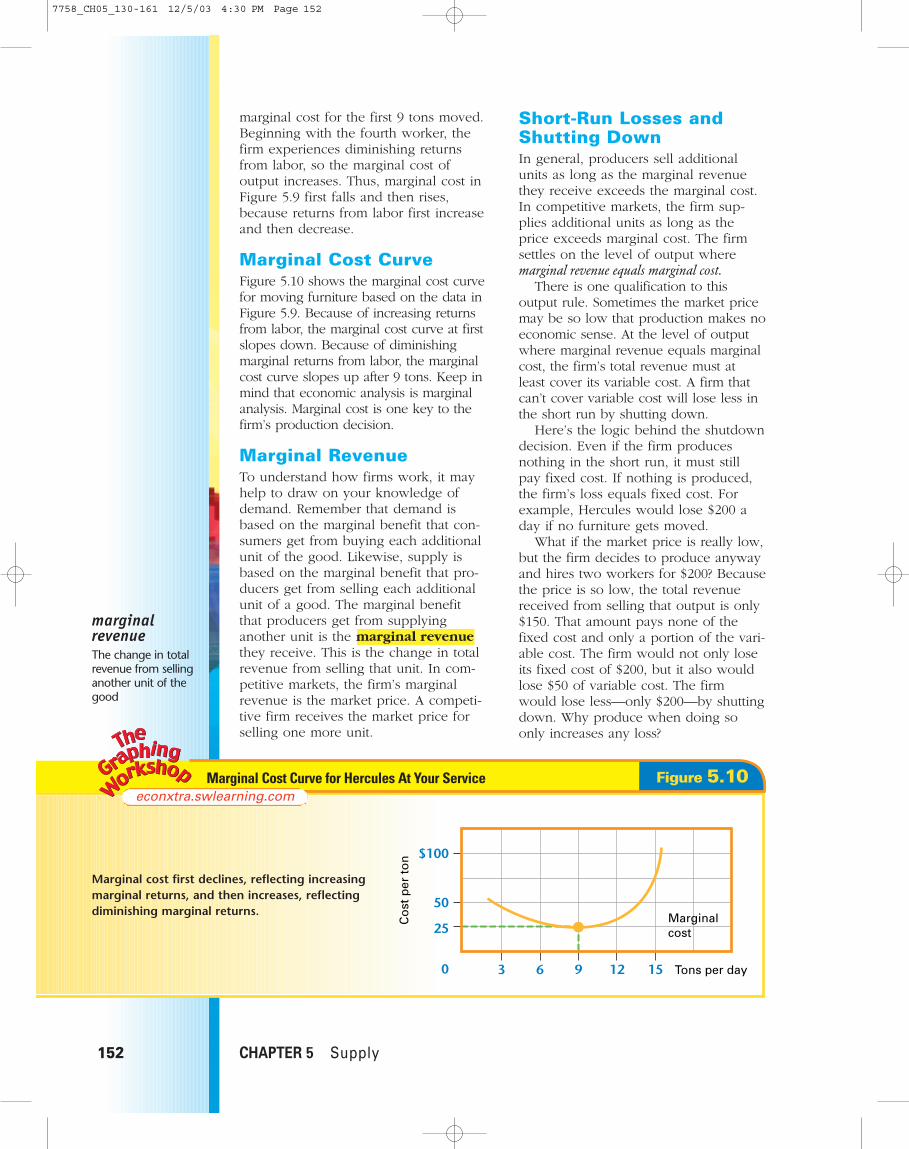
Marginal Cost Curve Figure 5.10 shows the marginal cost curvefor moving furniture based on the data inFigure 5.9. Because of increasing returnsfrom labor, the marginal cost curve at firstslopes down. Because of diminishingmarginal returns from labor, the marginalcost curve slopes up after 9 tons. Keep inmind that economic analysis is marginalanalysis. Marginal cost is one key to thefirm’s production decision.
Marginal RevenueTo understand how firms work, it mayhelp to draw on your knowledge ofdemand. Remember that demand isbased on the marginal benefit that con-sumers get from buying each additionalunit of the good. Likewise, supply isbased on the marginal benefit that pro-ducers get from selling each additionalunit of a good. The marginal benefitthat producers get from supplyinganother unit is the marginal revenuethey receive. This is the change in totalrevenue from selling that unit. In com-petitive markets, the firm’s marginalrevenue is the market price. A competi-tive firm receives the market price forselling one more unit.
Short-Run Losses andShutting Down In general, producers sell additionalunits as long as the marginal revenuethey receive exceeds the marginal cost.In competitive markets, the firm sup-plies additional units as long as theprice exceeds marginal cost. The firmsettles on the level of output wheremarginal revenue equals marginal cost.
There is one qualification to thisoutput rule. Sometimes the market pricemay be so low that production makes noeconomic sense. At the level of outputwhere marginal revenue equals marginalcost, the firm’s total revenue must atleast cover its variable cost. A firm thatcan’t cover variable cost will lose less inthe short run by shutting down.
Here’s the logic behind the shutdowndecision. Even if the firm producesnothing in the short run, it must stillpay fixed cost. If nothing is produced,the firm’s loss equals fixed cost. Forexample, Hercules would lose $200 aday if no furniture gets moved.
What if the market price is really low,but the firm decides to produce anywayand hires two workers for $200? Becausethe price is so low, the total revenuereceived from selling that output is only$150. That amount pays none of thefixed cost and only a portion of the vari-able cost. The firm would not only loseits fixed cost of $200, but it also wouldlose $50 of variable cost. The firmwould lose less—only $200—by shuttingdown. Why produce when doing soonly increases any loss?
152 CHAPTER 5 Supply
marginalrevenue The change in totalrevenue from sellinganother unit of thegood
Marginal cost first declines, reflecting increasingmarginal returns, and then increases, reflectingdiminishing marginal returns.
econxtra.swlearning.comFigure 5.10Marginal Cost Curve for Hercules At Your Service
63 9 12 150
$100
50
25
Tons per day
Marginalcost
Co
st p
er t
on
7758_CH05_130-161 12/5/03 4:30 PM Page 152

A firm’s minimum acceptable price is aprice high enough to ensure that totalrevenue at least covers variable cost. If the market price is below thatminimum, the firm will shut down. Notethat shutting down is not the same asgoing out of business. A firm that shutsdown keeps its productive capacityintact—paying the rent, fire insurance,and property taxes, keeping water pipesfrom freezing in the winter, and so on.For example, auto factories sometimesshut down for a while when sales aresoft. Businesses in summer resorts oftenclose for the winter. These firms do notescape fixed cost by shutting down,because fixed cost by definition is notaffected by changes in output.
If in the future the price increasesenough, the firm will resume produc-tion. If market conditions look grim andare not expected to improve, the firmmay decide to leave the market. Butthat’s a long-run decision. The short runis defined as a period during whichsome resources and some costs arefixed. A firm cannot escape those costsin the short run, no matter what it does.The firm cannot enter or leave themarket in the short run.
The Firm’s Supply Curve To produce in the short run, the pricemust be high enough to ensure that totalrevenue covers variable cost. The com-petitive firm’s supply curve is the
upward sloping portion of its marginalcost curve at and above the minimumacceptable price. This supply curveshows how much the firm will supply ateach price.
In the Hercules example, a price of$33.33 allows the firm to at least covervariable cost. Hercules’s short-runsupply curve is presented in Figure 5.11as the upward-sloping portion of themarginal cost curve starting at $33.33. Atthat price, Hercules will supply 12 tonsof moving a day. At a price of $50 perton, the company will move 14 tons,and at a price of $100 per ton, thecompany will move 15 tons. The marketsupply curve sums individual supplycurves for firms in the market.
Production andCosts in theLong RunSo far, the analysis has focused on howshort-run costs vary with output for afirm of a given size. In the long run, all
competitivefirm’s supplycurveThe rising portion ofa firm’s marginal costcurve at or above theprice that will allowthe firm to covervariable cost
Lesson 5.3 Production and Cost 153
A competitive firm’s supply curve shows thequantity supplied at each price. The supplycurve is the upward-sloping portion of itsmarginal cost curve, beginning at the firm’sminimum acceptable price. The minimumacceptable price, in this case $33.33, is theprice that allows the firm’s total revenue tocover its variable cost.
Figure 5.11Supply Curve for Hercules at Your Service
12 14 150
$100.00
50.00
33.33
Tons per day
Co
st p
er t
on
Supply
Why does the firm’s marginal costcurve slope upward in the shortrun?
C H E C K P O I N T
7758_CH05_130-161 12/5/03 4:30 PM Page 153

inputs can be varied, so there are nofixed costs. What should be the size ofthe firm?
Economies of ScaleBecause all resources can vary in thelong run, the focus is on the averagecost of production, not the marginalcost. Average cost equals total costdivided by output. The firm’s ownerwould like to know how the averagecost of production varies as the size,or scale, of the firm increases. A firm’slong-run average cost indicates the lowestaverage cost of producing each outputwhen the firm’s size is allowed to vary.
If the firm’s long-run average costdeclines as the firm size increases, thisreflects economies of scale. Considersome reasons for economies of scale. Alarger-size firm often allows for larger, more spe-cialized machines and greater specialization oflabor. Typically, as the scale of the firmincreases, capital substitutes for labor.Production techniques such as theassembly line can be introduced only ifthe firm is sufficiently large.
Diseconomies of ScaleAs the scale of the firm continues
to increase, however, anotherforce may eventually takehold. If the firm’s long-runaverage cost increases as pro-
duction increases, this reflects dis-economies of scale. As the amount and
variety of resources employed increase,so does the task of coordinating all theseinputs. As the workforce grows, additionallayers of management are needed tomonitor production. Information may notbe correctly passed up or down thechain of command.
It is possible for long-run average costto neither increase nor decrease withchanges in firm size. If neither economiesof scale nor diseconomies of scale occuras the scale of the firm expands, a firmexperiences constant returns to scale oversome range of production.
Long-Run Average CostCurveFigure 5.12 presents a firm’s long-runaverage cost curve, showing thelowest average cost of producing eachlevel of output. The curve is markedinto segments reflecting economies ofscale, constant returns to scale, and dis-economies of scale. Production mustreach quantity A for the firm to achievethe minimum efficient scale, which is thesmallest scale, or size, that allows thefirm to take full advantage of economiesof scale. At the minimum efficient scale,long-run average cost is at a minimum.From output A to output B, the firmexperiences constant returns to scale.Beyond output rate B, diseconomies ofscale increase long-run average cost.
Firms try to avoid diseconomies ofscale. Competition weeds out firms thatgrow too large. To avoid diseconomiesof scale, IBM divided into six smallerdecision-making groups. Other largecorporations have spun off parts of theiroperations to create new companies. HPstarted Agilent Technologies, and AT&Tstarted Lucent Technologies.
The long-run average cost curveguides the firm toward the most effi-cient plant size for a given level ofoutput. However, once a plant of thatscale is built, the firm has fixed costsand is operating in the short run. A firmin the short run chooses the output ratewhere marginal revenue equals mar-ginal cost. Firms plan for the long run,but they produce in the short run.
154 CHAPTER 5 Supply
long-runaverage costcurve A curve that indi-cates the lowestaverage cost of pro-duction at each rateof output when thefirm’s size is allowedto vary
economies ofscaleForces that reduce afirm’s average cost asthe firm’s size, orscale, increases in thelong run
THE WALL STREET JOURNALReading It Right What’s the relevance of the fol-lowing statement from The Wall Street Journal: “As with any newtechnology, the early OLED (organic light-emitting diode) displayscreens are expensive, perhaps six times more than liquid-crystal-display screens. But OLED backers say that problem will in partbe addressed once mass production gears up and economies ofscale are reached.”
How are economies of scale anddiseconomies of scale reflected ina firm’s long-run average costcurve?
C H E C K P O I N T
Economic Healtheconxtra.swlearning.com
®video
7758_CH05_130-161 12/5/03 4:30 PM Page 154

Lesson 5.3 Production and Cost 155
Average cost declines until productionreaches output level A. The firm isexperiencing economies of scale. Outputlevel A is the minimum efficient scale—thelowest rate of output at which the firm takes full advantage of economies of scale.Between A and B, the economy has constantreturns to scale. Beyond output level B,the long-run average cost curve reflectsdiseconomies of scale.
Figure 5.12A Firm’s Long-Run Average Cost Curve
BA0 Output per period
Long-runaverage cost
Economiesof scale
Constantreturnsto scale
Diseconomiesof scale
Co
st p
er u
nit
Worker’s Compensation All across thenation, the cost of worker’s compensationinsurance has been spiking upward at a fright-ening rate. A seafood wholesaler in LosAngeles saw its rates climb 68 percent in oneyear to almost $7,000 per employee. Mostinsurance costs have risen for companies in thepast few years, but “worker’s comp,” as it isoften called, is a major problem because firmshave no control over cost increases. By law,companies must provide worker’s comp insur-ance, which pays for medical treatment for job-related injuries and for wages lost as a result ofthose injuries. Because every employee musthave worker’s comp insurance, the only way acompany can reduce this cost is to eliminateemployees. Increased insurance costs havecaused both large and small companies to lay
off workers, and—in many cases—it has forcedthem out of business. The main reasons for thesharp increases in worker’s comp costs aresoaring medical and legal costs, and fraud.Workers fake injuries and stay out of worklonger than necessary. Doctors, chiropractors,and lawyers work together to cheat thesystem. Companies also manipulate theiremployee reports and downplay the dangersinvolved in the work that’s being done in orderto pay less than they should.
Think CriticallyWhat are the ethical issues involved withworker’s compensation insurance? How doesthe increase in worker’s compensation insur-ance affect a firm’s long-run average costcurve?
7758_CH05_130-161 12/5/03 4:30 PM Page 155
Key Concepts1. Tanya runs a computer repair business in a small room in her basement. Many
people wanted her to fix their computers so she hired another worker, whodoubled the number of computers she could fix each day. But when she hired athird worker, she found that the number of computers she could service hardlychanged at all. Explain how this demonstrates the law of diminishing returns.
2. Tanya has borrowed more than $10,000 to buy special equipment she needs inorder to repair computers. Is the $750 she pays each month to repay her loan afixed or a variable cost? Explain your answer.
3. Tanya pays her worker $15.00 per hour. If, on average, he can repair one com-puter in two hours, what is the marginal cost of fixing one more computer?What other information does she need to have before she can decide howmuch to charge her customers for computer repairs?
4. Tanya’s monthly fixed costs total $1,000. She pays her assistant $2,500 eachmonth. She could take a job with a different business that would pay her$3,000 each month. Her total revenue from sales last month amounted to$6,000. Should she continue to operate the business or shut it down?
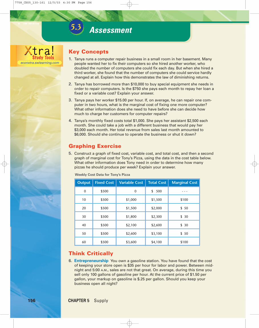
Graphing Exercise5. Construct a graph of fixed cost, variable cost, and total cost, and then a second
graph of marginal cost for Tony’s Pizza, using the data in the cost table below.What other information does Tony need in order to determine how manypizzas he should produce per week? Explain your answer.
Think Critically6. Entrepreneurship You own a gasoline station. You have found that the cost
of keeping your store open is $35 per hour for labor and power. Between mid-night and 5:00 A.M., sales are not that great. On average, during this time yousell only 100 gallons of gasoline per hour. At the current price of $1.50 pergallon, your markup on gasoline is $.25 per gallon. Should you keep yourbusiness open all night?
156 CHAPTER 5 Supply
Weekly Cost Data for Tony’s Pizza
Output Fixed Cost Variable Cost Total Cost Marginal Cost
0 $500 $1,000 $1,500 - - -
10 $500 $1,000 $1,500 $100
20 $500 $1,500 $2,000 $150
30 $500 $1,800 $2,300 $130
40 $500 $2,100 $2,600 $130
50 $500 $2,600 $3,100 $150
60 $500 $3,600 $4,100 $100
Assessment5.3
econxtra.swlearning.com
7758_CH05_130-161 12/5/03 4:30 PM Page 156

absoluteadvantage To be able tomake somethingusing fewerresources thanother producersrequire
to HistoryC O N N E C T
The increases in the production of cotton tex-tiles in the late 1700s brought about theIndustrial Revolution. As production becamemore industrialized, suppliers of raw cottonwere faced with heavy demand. In the UnitedStates, growing cotton was profitable only alonga narrow strip along the coast of Georgia andthe Carolinas. It was the only place Sea Islandcotton could be grown. Another strain, whichcould be grown in the interior, was unprofitablebecause it produced a lot of seeds, which couldbe removed only by hand. It took a day’s workto separate the seeds from the lint, making ittoo slow and too expensive to satisfy thedemands of the industry.
Eli Whitney changed all this in 1793 withhis invention of the cotton gin. Whitney’sinvention allowed one man to produce what ithad previously taken 50 men, mostly slaves, toproduce. Cotton now could be grown where itformerly had been cost prohibitive, enabling theAmerican South to supply Great Britain’sgrowing demand for raw cotton. Within twoyears, cotton exports from the United States toGreat Britain rose from 487,000 pounds to6,276,300. Because Great Britain’s textile millswere demanding ever-increasing amounts ofcotton, Southern planters were willing to moveinland and devote more land and resources toproducing cotton. The quantity of cotton sup-plied increased rapidly, keeping pace with thegrowing British cotton textile industry.
The British government, protective of itstextile industry, passed laws preventing anyonewith knowledge of the workings of a textilemill from leaving the country. Despite thatprohibition, an English textile mechanic,Samuel Slater, was attracted by a prize beingoffered for information about the Englishtextile industry. He disguised himself as a farmlaborer and came to the United States. Slaterestablished a mill at Pawtucket, Rhode Island.Building its machinery entirely from memory,he started the American textile industry onDecember 20, 1790. Still, American mills hada difficult time competing with Britishimports and could afford only cheaper cottonimported from the West Indies. Southernstates sold all of their cotton at a better price toEnglish mills.
THINK CRITICALLYWhat variable cost did the invention of thecotton gin allow Southern cotton producers tolower? How were the growers able to create“economies of scale”? Why do you think theAmerican cotton mills, using essentially thesame equipment, had difficulty competingwith the British cotton imports?
to HistoryIndustrial Revolution in the United States:The Supply of CottonThe
Lesson 5.3 Production and Cost 157
7758_CH05_130-161 12/5/03 4:30 PM Page 157

158 CHAPTER 5 Supply
SummaryThe Supply Curve
a Firms are motivated to produce products outof their desire to earn profit. Supply indicateshow much of a good producers are willingand able to offer for sale per period at each
possible price, other thingsconstant. The law ofsupply states that thequantity of a product sup-plied will be greater at a
higher price than at a lower price, other thingsconstant.
b Businesses supply more products at higherprices because they can shift resources fromthe production of other products that havelower prices. Further, higher prices encourageproducers to find new sources of resources,or more efficient means of production.Individual supply is the quantity of productsupplied by one firm in a market. Marketsupply is the total quantity of product sup-plied by all firms in a market.
c The price elasticity of supply is the relationshipbetween a percentage change in the price of aproduct and the resulting percentage changein the quantity supplied. Supply may beelastic, unit elastic, or inelastic. As a generalrule, the more difficult or costly it is to changethe quantity of a product produced, the lesselastic supply will be.
Shifts of the Supply Curve
a There are five determinants of supply thatshift the location of a supply curve when theychange. They are (1) changes in the cost ofresources used to make the good, (2) changesin the price of other goods these resourcescould make, (3) changes in the technologyused to make the good, (4) changes in theproducers’ expectations, and (5) changes inthe number of sellers in the market.
b A change in the price of a product will causemovement along a supply curve that is called
a change in the quantity supplied. A changein a determinant of supply will cause a supplycurve to move or shift to the left or right.
Production and Cost
a Production in the short run takes place in aperiod during which at least one productiveresource cannot be changed or is fixed.Variable resources may be changed in theshort run. In the long run, all resources arevariable.
b The marginal product of an additional workeris the change in total production that resultsfrom employing one more worker. When pro-duction of a product is increased, there aretypically first increasing returns and thendiminishing returns.
c Fixed cost must be paid in the short run anddoes not change with the quantity produced.Variable cost is zero when output is zero andincreases when output increases.
d Marginal cost equals the change in total costdivided by the change in total quantity.Marginal revenue is the additional revenueresulting from selling one more unit ofoutput. Businesses will sell more output aslong as the marginal revenue exceeds themarginal cost. In the short run, a firm’ssupply curve is that portion of its marginalcost curve rising above the minimum accept-able price.
e In the short run, firms that are losing moneywill continue to produce as long as their totalrevenue is greater than their variable cost. If they shut down, they would lose morethan they would if they continued to makeproducts.
f In the long run, firms face economies and dis-economies of scale. The long-run averagecost curve first slopes downward as the scaleof the firm expands, reflecting economies ofscale. At some point it may flatten out, reflect-ing constant returns to scale. As the scale ofthe firm increases, the long-run average costcurve may begin to slope upward, reflectingdiseconomies of scale.
Chapter Assessment55.1
5.3
5.2
econxtra.swlearning.com
7758_CH05_130-161 12/5/03 4:30 PM Page 158

Chapter Assessment 159
Review Economic TermsChoose the term that best fits the definition. On a separate sheet of paper, write theletter of the answer. Some terms may not be used.
1. A period of time during which at least one of afirm’s resources is fixed
2. The change in total revenue from selling anotherunit of a product
3. Any cost that does not change with the amountof production in the short run
4. A period of time during which all of a firm’sresources can be varied
5. The change in total cost resulting from producingone more unit of output.
6. Any production cost that changes as outputchanges
7. A measure of the responsiveness of the quantityof a product supplied to a change in price
8. The change in total product that results from anincrease of one unit of resource input
9. As more of a variable resource is added to a givenamount of fixed resources, marginal producteventually declines and could become negative
10. Forces that reduce a firm’s average cost as thefirm’s size grows
11. The total output of the firm
a. competitive firm’s supply curve
b. economies of scale
c. elasticity of supply
d. fixed cost
e. law of diminishing returns
f. law of supply
g. long run
h. long-run average cost curve
i. marginal cost
j. marginal product
k. marginal revenue
l. short run
m. supply
n. supply curve
o. total cost
p. total product
q. variable cost
Review Economic Concepts12. A shift of a product’s supply curve will be
caused by each of the following except
a. an increase in the cost of the resourcesused to produce the product.
b. an improvement in the technology usedto produce the product.
c. an increase in consumer demand for theproduct.
d. a decrease in the price of other productsthat resources could be used to produce.
13. True or False If a product’s elasticity ofsupply is 0.8, a 2 percent increase in price willcause a greater than 2 percent increase in thequantity supplied.
14. Typically, the longer the period of time, the__?__ a product’s elasticity of supply will be.
15. Which of the following events would cause thesupply curve to shift to the left?
a. A firm’s employees negotiate a 5 percentincrease in their wages.
b. A firm’s managers buy new, more effi-cient machinery for workers to use.
c. A firm provides its workers with trainingto better use their tools.
d. A firm finds a new, less expensive sourceof raw materials.
7758_CH05_130-161 12/5/03 7:23 PM Page 159
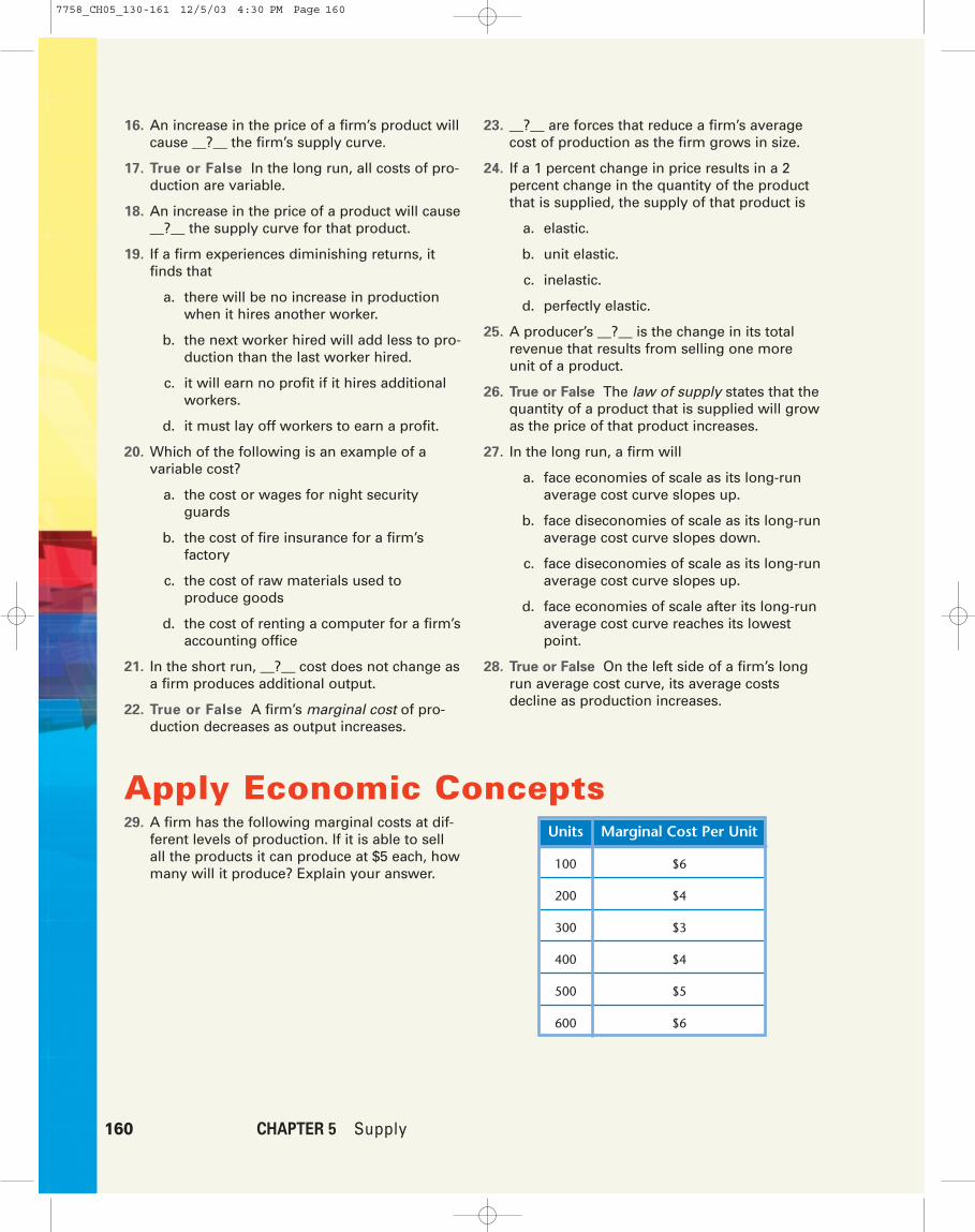
160 CHAPTER 5 Supply
16. An increase in the price of a firm’s product willcause __?__ the firm’s supply curve.
17. True or False In the long run, all costs of pro-duction are variable.
18. An increase in the price of a product will cause__?__ the supply curve for that product.
19. If a firm experiences diminishing returns, itfinds that
a. there will be no increase in productionwhen it hires another worker.
b. the next worker hired will add less to pro-duction than the last worker hired.
c. it will earn no profit if it hires additionalworkers.
d. it must lay off workers to earn a profit.
20. Which of the following is an example of a variable cost?
a. the cost or wages for night securityguards
b. the cost of fire insurance for a firm’sfactory
c. the cost of raw materials used to produce goods
d. the cost of renting a computer for a firm’saccounting office
21. In the short run, __?__ cost does not change asa firm produces additional output.
22. True or False A firm’s marginal cost of pro-duction decreases as output increases.
23. __?__ are forces that reduce a firm’s averagecost of production as the firm grows in size.
24. If a 1 percent change in price results in a 2percent change in the quantity of the productthat is supplied, the supply of that product is
a. elastic.
b. unit elastic.
c. inelastic.
d. perfectly elastic.
25. A producer’s __?__ is the change in its totalrevenue that results from selling one moreunit of a product.
26. True or False The law of supply states that thequantity of a product that is supplied will growas the price of that product increases.
27. In the long run, a firm will
a. face economies of scale as its long-runaverage cost curve slopes up.
b. face diseconomies of scale as its long-runaverage cost curve slopes down.
c. face diseconomies of scale as its long-runaverage cost curve slopes up.
d. face economies of scale after its long-runaverage cost curve reaches its lowestpoint.
28. True or False On the left side of a firm’s longrun average cost curve, its average costsdecline as production increases.
Apply Economic Concepts29. A firm has the following marginal costs at dif-
ferent levels of production. If it is able to sellall the products it can produce at $5 each, howmany will it produce? Explain your answer.
Units Marginal Cost Per Unit
100 $6
200 $4
300 $3
400 $4
500 $5
600 $6
7758_CH05_130-161 12/5/03 4:30 PM Page 160

Chapter Assessment 161
30. The lowest long-run average cost for whatsits is$50 per unit. To take advantage of economies ofscale and produce whatsits at this low cost, afirm would need to build a factory that couldproduce 5,000,000 whatsits per year. There areonly 20,000 people who are willing to pay any-thing to buy a whatsit per year. Why won’t alarge whatsits factory be built?
31. Calculating the Price Elasticity of Supply
Complete the table below by calculating eachmissing elasticity of supply value. Is the supplyelastic or inelastic?
32. Sharpen Your Life Skills: Cause and Effect
During the summer of 2003, Americans werewarned that shortages of natural gas couldcause its price to increase by as much as 50percent or more during the following winter.Natural gas is a primary ingredient used in theproduction of artificial fertilizer. Much of thefertilizer used by U.S. farmers during thespring of 2004 was produced during the pre-ceding winter. If the cost of producing this fer-tilizer increased as predicted, what would havehappened to the location of the supply curvefor agricultural products in 2004? Explain youranswer.
33. Accounting Classify each of the followingcosts as variable or fixed. Explain your deci-sion for each cost.
• The cost of a leased delivery truck
• The cost of a night security service
• The cost of delivering finished products
• The cost of fire insurance
• The cost of electricity used to run produc-tion machinery
34. Access EconData Online at econxtra.swlearning.com. Read the article entitled“Labor Cost Per Unit of Output.” Find theanswers to the following questions from thearticle: (1) What is the relationship betweenlabor productivity and worker’s compensationinsurance? (2) Why is labor cost an importantindicator of trends in production costs? Writeyour answers in complete sentences on a sheetof paper.
econxtra.swlearning.com
Price Elasticity of Supply for Dozens of Bagels
Percentage Quantity Percentage
Price Change Supplied Change Elasticity Elastic/Inelastic
$8 - - - 100 - - - - - - - - -
$7 12.5% 90 10.0% ______ ______
$6 14.3% 80 11.1% ______ ______
$5 16.6% 70 12.5% ______ ______
$4 20.0% 60 14.3% ______ ______
$3 25.0% 50 16.6% ______ ______
7758_CH05_130-161 12/5/03 7:23 PM Page 161