7/d user's manual for the heat pipe space radiator design ... · pdf fileuser manual for...
TRANSCRIPT

I/
NASA Contxactor Report 187067 "7/d/ •
i / /"
User's Manual for the Heat Pipe Space
Radiator Design and Analysis _Code (HEPSPARC)
G i,/i t.$
N9 i-2 _"3 g"...
Donald C. HainleySverdrup Technology, Inc.
Lewis Research Center GroupBrook Park, Ohio
April 1991
Prepared forLewis Research Center
Under Co_,tract NAS3-25266
National Aero"tautics and
Space Admit ,.,.:ration
https://ntrs.nasa.gov/search.jsp?R=19910013045 2018-04-28T22:38:55+00:00Z

User Manual
for the
Multi-Purpose Heat Pipe Space Radiator
Design and Analysis Code (HEPSPARC)
Code Version 1.0
by
Donald C. Hainley
Sverdrup Technology, Inc.
Lewis Research Center Group
Brook Park, Ohio 44142
September 17, 1990
Synopsis:
A new computer code has been written for the NASA Lewis Research Center
named HEPSPARC (which stands for HE_._atPipe SP___AAceRadiator C_ode). This code is
used for the design and analysis of a radiator that is constructed from a
pumped fluid loop that transfers heat to the evaporative section of heatpipes.
This manual is designed to familiarize the user with this new code and to
serve as a reference for its use. This manual documents the work done thus
far. It is also intended to be the first step towards verification of theHEPSPARC code.
Details are furnished to provide a description of all the requirements
and variables used in the design and analysis of a combined pumped loop/heat
pipe radiator system. A description of the subroutines used in the program is
furnished for those interested in understanding its detailed workings.


Table of Contents
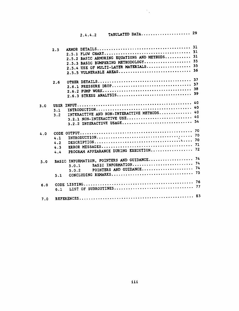
LIST OF FIGURES ........................................... iv
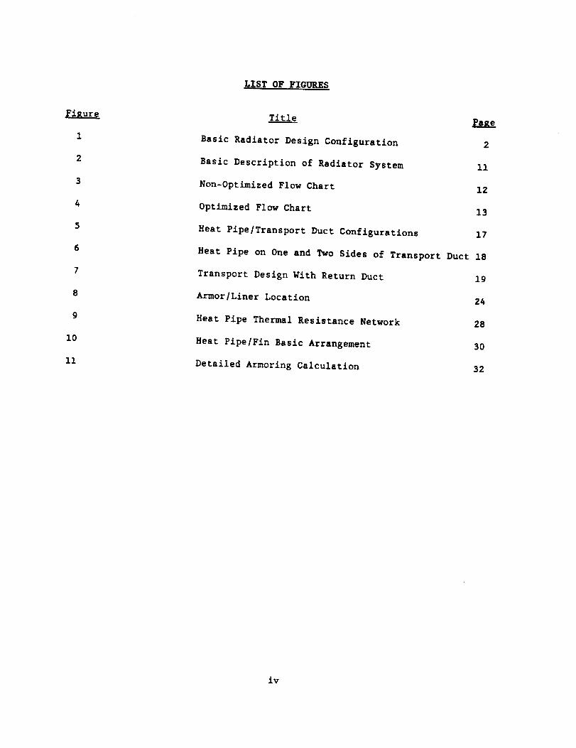
LIST OF TABLES ............................................ v
1.0 GENERAL OVERVIEW .......................................... 1
i.I INTRODUCTION ........................................ 1
1.2 CODE DESCRIPTION/USAGE .............................. i
1.3 CODE HIGHLIGHTS/DETAIL .............................. 3
1.4 PURPOSE OF MANUAL................................... 6
2.0 CODE DETAILS .............................................. 7
2.1 GENERAL ............................................. 7
2.1.1 OPERATING SYSTEM .............................. 7
2.1.2 BASIC PROCEDURES .............................. 7
2.1.3 GENERAL FLOW CHART ............................ 10
2.1.4 DESCRIPTION OF CODE WORKINGS .................. i0
2.1.4.1 NON-0PTIMIZED METHOD .............. 10
2.1.4.2 OPTIMIZED APPROACH ................ 14
2.2 GEOMETRY POSSIBILITIES .............................. 15
2.2.1 TRANSPORT DUCT ................................ 16
2.2.2 HEAT PIPES .................................... 16
2.3 MATERIALS ........................................... 20
2.3.1 FLUIDS ........................................ 20
2.3.1.1 TRANSPORT DUCT .................... 20
2.3.1.2 HEAT PIPE ......................... 21
2.3.2 METALS ........................................ 21
2.3.2.1 LINERS/ARMORS/FINS/WICKS .......... 21
2.3.2.2 BUMPERS ........................... 23
2.3.2.3 COMPATIBILITY INFORMATION ......... 23
2.3.2.4 LINEKS ............................ 23
2.5.2.5 PROPERTIES ........................ 25
2.4 HEAT TRANSFER DETAILS ........... _.................... 25
2.4.1 OVERVIEW ...................................... 25
2.4.2 TRANSPORT DUCT FLUID .......................... 25
2.4.2.1 BASIC EQUATIONS ................... 252.4.2.2 AREA MULTIPLIER ................... 26
2.4.3 HEAT PIPE ..................................... 27
2.4.3.1 EVAPORATOR/CONDENSER .............. 27
2.4.4 FINS .......................................... 27
2.4.4.1 GRAY BODY ANALYSIS ................ 29
ii
2.4.4.2 TABULATED DATA ..................... 29
3.0
4.0
5.0
6.0
7.0
2.5 ARMOR
2.5.1
2.5.2
2.5,3
2.5.4
2.5.5
DETAILS ........................................ 31
FLOW CHART ..................................... 31
BASIC ARMORING EQUATIONS AND METHODS ........... 31
BASIC BUMPERING METHODOLOGY .................... 35
USE 0FMULTI-LAYEEMATEEIALS ................... 35
VULNERABLE AREAS ............................... 36
2.6 OTHER
2.6.1
2.6.2
2.6.3
DETAILS ........................................ 37
PRESSURE DROP .................................. 37
PUMP WORK ...................................... 38
STRESS ANALYSIS ................................ 39
USER INPUT ................................................. 40
3.1 INTRODUCTION ......................................... 40
3.2 INTERACTIVE AND NON-INTERACTIVE METHODS .............. 40
3.2.1 NON-INTERACTIVE USE ............................ 40
3.2.2 INTERACTIVE USAGE .............................. 56
CODE OUTPUT ................................................ 70
4.1 INTRODUCTION ......................................... 70
4.2 DESCRIPTION ..................................... : .... 70
4.3 ERROR MESSAGES ....................................... 71
4.4 PROGRAM APPEARANCE DURING EXECUTION .................. 72
BASIC
5.1
INFORMATION, POINTERS AND GUIDANCE ................... 74
5.0.1 BASIC INFOEMATION .......................... 74
5.0.2 POINTERS AND GUIDANCE ...................... 74
CONCLUDING REMARKS ................................... 75
CODE LISTING ............................................... 76
6.i LIST OF SUBROUTINES .................................. 77
REFERENCES ................................................. 83
iii
1
2
3
4
5
6
7
8
9
10
11
LIST OF FIGURES
Title
Basic Radiator Design Configuration
Basic Description of Radiator System
Non-Optimized Flow Chart
Optimized FlowChart
Heat Pipe/Transport Duct Configurations
2
11
12
13
17
Heat Pipe on One and Two Sides of Transport Duct 18
Transport Design With Return Duct
Armor/Liner Location
Heat Pipe Thermal Resistance Network
Heat Pipe/Fin Basic Arrangement
Detailed Armoring Calculation
19
24
28
30
32
iv
Table
3.
2
3
4
5
LIST OF TABLES
Titl__.__E
Inputs and User Options
HEPSPARC Output
Transport Duct Fluids
Heat Pipe Fluids
Materials for Liners, Armor, Fins, and Wicks
4
5
20
21
22
V
i.___O0 GENERAL OVERVIEW:
l.__.! INTRODUCTION:
The demand for increased spacecraft power brings with it a rise in waste
heat rejection requirements due to power conversion system inefficiencies.
This growth of power systems necessitates the ability to analyze the numerous
radiator possibilities available to meet the requirements. The most efficient
method to meet the specifications must be determined from the existing
options. Thus, analytical modeling tools have become a requirement for power
system heat transfer analysis, optimization, and comparison.
Existing spacecraft heat transfer systems are primarily composed of
pumped loop systems (i), heat pipe systems (2), or combinations of the two,
while advanced, low mass systems are also being developed (3,4,5) as
alternatives. Current radiator designs show an increasing dependence on
systems employing heat pipes. The growing dependency on heat pipes is in part
due to the nearly isothermal character and high heat transfer capabilities
inherent in the heat pipe concept. The increased dependence is also due to the
fact that each heat pipe of a radiator system can be considered an independent
entity. A designer can plan for heat pipe failures due to environmental
hazards over the radiator life without concern for overall heat rejection
system failure. Both these facts allow a heat pipe radiator to typically
become lighter and smaller than a comparable pumped loop system.
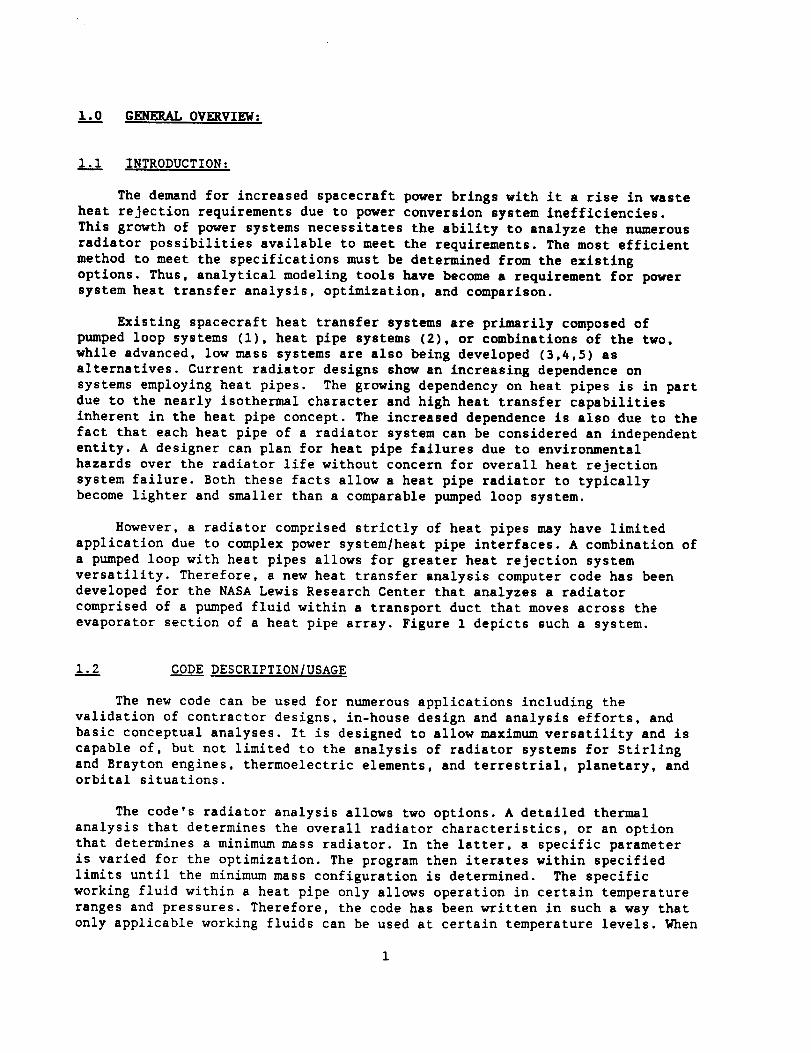
However, a radiator comprised strictly of heat pipes may have limited
application due to complex power system/heat pipe interfaces. A combination of
a pumped loop with heat pipes allows for greater heat rejection system
versatility. Therefore, a new heat transfer analysis computer code has been
developed for the NASA Lewis Research Center that analyzes a radiator
comprised of a pumped fluid within a transport duct that moves across the
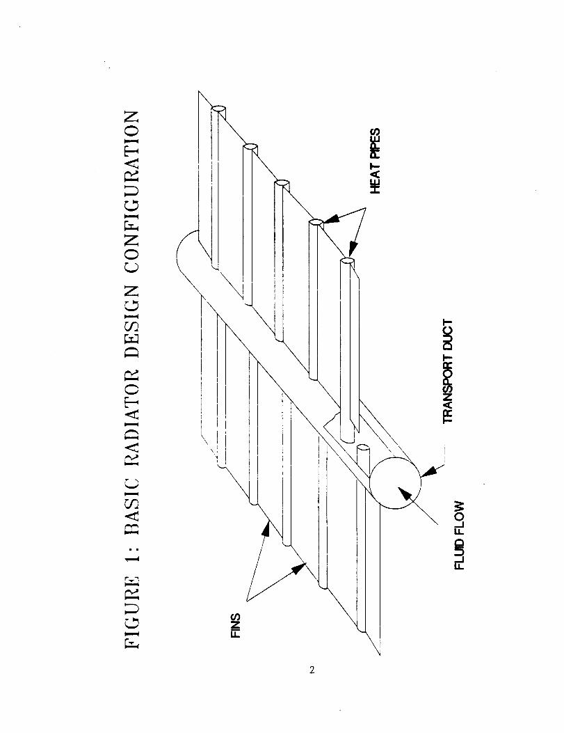
evaporator section of a heat pipe array. Figure 1 depicts such a system.
i.__! CODE DESCRIPTION/USAGE
The new code can be used for numerous applications including the
validation of contractor designs, in-house design and analysis efforts, and
basic conceptual analyses. It is designed to allow maximum versatility and is
capable of, but not limited to the analysis of radiator systems for Stifling
and Brayton engines, thermoelectric elements, and terrestrial, planetary, and
orbital situations.
The code's radiator analysis allows two options. A detailed thermal
analysis that determines the overall radiator characteristics, or an option
that determines a minimum mass radiator. In the latter, a specific parameter
is varied for the optimization. The program then iterates within specified
limits until the minimum mass configuration is determined. The specific
working fluid within a heat pipe only allows operation in certain temperature
ranges and pressures. Therefore, the code has been written in such a way that
only applicable working fluids can be used at certain temperature levels. When
Z
o
Z0
Z
C¢2
0
OQ
I,I.
T
\
\
I
\j\
\
2

the radiator must produce a large temperature change in the pumped loop fluid,
the code indexes through different heat pipes chosen for the design. The
temperature of a particular heat pipe is checked against specified limits to
determine its acceptability at a particular radiator location. If the heat
pipe is found to be operating at or over a limit, a heat pipe with a different
working fluid will be chosen. This capability allows the program to be used
for the design and analysis of radiators that require a large temperature drop
in the transport duct fluid. A radiator for a Brayton cycle system presents
such a situation. The optimization option also accounts for multiple heat pipe
types in its calculations and allows independent optimizing calculations of
each heat pipe type to minimize the entire radiator mass.
One of the most important aspects of a design for a space based radiator
system is the manner in which it is protected from the space environment. The
protection method used is referred to as armoring or bumpering. The
determination of the required armoring in the code follows the methodology
described in Reference (6). It uses an iterative technique to balance the
number of allowable losses of heat pipes or transport ducts with that
predicted by an assumed armor thickness using a "critical particle flux".
Particle impact effects are accounted for by the choice of two models: the
NASA thick plate, with specified adjustment factors (7,8), or the NASA thin
plate model (8). Armoring thickness is adjusted until the design specified
number of heat pipe losses is at its maximum allowable value. This technique
allows the analyst to account for the radiator environmental conditions. It
also allows a reduced mass design by use of redundancy in the heat pipes as
well as with the transport ducts. Additional program options will allow the
use of offset bumpering as transport duct protection.
I._! COD.___EHIGHLIGHTS_DETAIL:
The complexity and generality of this program causes its input to be
detailed. Table 1 summarizes the input and user options available. An
adequate knowledge of heat pipes is needed to specify all the required
parameters. Basic understanding of space radiator design is also necessary to
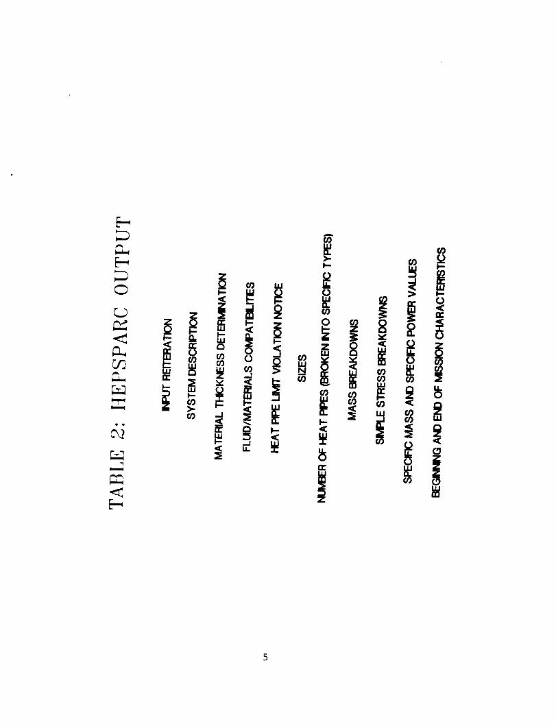
make maximum use of the program. A significant amount of detail about the
radiator is returned from the code analysis (see Table 2). When the
optimization option is used, information about the iterative step values is
also output in order to track the minimization process.
The code offers many unique features, A built-in library offers the
designer a wide selection of radiator materials. The option of using
properties not already in the library by allowing user defined properties is
also available. This allows a designer to easily determine the relative impact
of new materials on a radiator design. Data is also available within the
program to indicate known compatibility information between the materials
chosen for use.
Other program features include the use of fin and heat pipe efficiencies.
This accounts for the non-isothermal fin conditions as well as radiation
interchange between the fins and adjacent heat pipes.

ZDmmq
Any radiator geometry is easily modeled by using specified input and
options available. The basic configurations analyzed thus far include a simple
flat plate design, a cylindrical shape, and a conical shape. Each of these
configurations still allow for the use of all the program options previouslymentioned.
The basic structure of the radiator code's heat pipe analysis section is
based on portions of the NASA Lewis Heat Pipe Code (9). The technique employed
for evaluation of the heat pipe characteristics is an iteratlve method of
determining the thermal resistance and temperatures of the various sections of
the heat pipe. Essentially, a one-dimensional, lumped parameter, thermal
network model is used to obtain the heat transfer characteristics of the heat
pipes. Heat transfer limits are checked using fundamental equations available
in the literature.
The Lewis Heat Pipe Code allows for the use of a wide variety of heat
pipe wick structures. The choices available include wrapped screens, with or
without arteries, sintered metals, with or without arteries, and grooves. An
option also exists that allows the user to define all the parameters needed
for the thermal calculations. This provides the flexibility required to
evaluate new or different heat pipe concepts.
I.___4 PURPOSE O__V_IS_UAL
The new code, named HEPSPAEC, for HEat Pipe SP___AAceR_adiator Code, is very
generic in nature and allows for the design and analysis of a combined heat
pipe/pumped loop radiator for a wide variety of situations. This user manual
describes the usage, capabilities, and structure of this code. Details of all
aspects of the code will be described. Sufficient input requirements and
specifications will be provided to supply information to allow a new user to
work with the program.
This document allows users of various interest levels to pinpoint the
sections they may wish to read. As already seen, Section 1 has provided basic
overall description of the code and its application. Basic material involved
with the workings of the program is furnished in Section 2, while Section 3
details the requirements for actual usage of the code. Section 4 provides
information for understanding the code output as well as additional basic
information for its usage. Section 5 provides some final instructions and
guidance for the user. Section 6 contains (in the original version of this
manual only) a floppy disk with a copy of the program along with a description
of the subroutines involved in the code. Section 7 contains the list of
references for this document.
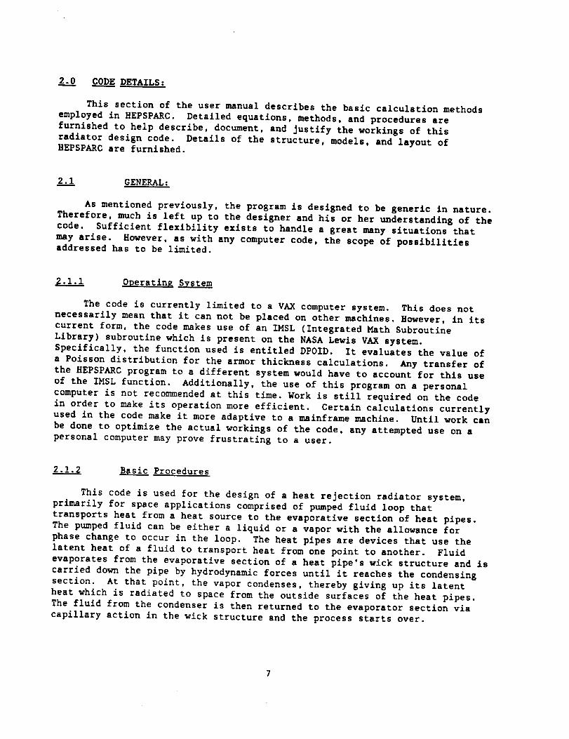
2.___O CODE DETAILS:
This section of the user manual describes the basic calculation methods
employed in HEPSPARC. Detailed equations, methods, and procedures are
furnished to help describe, document, and justify the workings of this
radiator design code. Details of the structure, models, and layout of
HEPSPARC are furnished.
2..._!i GENERAL:
As mentioned previously, the program is designed to be generic in nature.
Therefore, much is left up to the designer and his or her understanding of the
code. Sufficient flexibility exists to handle a great many situations that
may arise. However, as with any computer code, the scope of possibilities
addressed has to be limited.
2.1.1 Operating System
The code is currently limited to a VAX computer system. This does not
necessarily mean that it can not be placed on other machines. However, in its
current form, the code makes use of an IMSL (Integrated Math Subroutine
Library) subroutine which is present on the NASA Lewis VAX system.
Specifically, the function used is entitled DPOID. It evaluates the value of
a Poisson distribution for the armor thickness calculations. Any transfer of
the HEPSPARC program to a different system would have to account for this use
of the IMSL function. Additionally, the use of this program on a personal
computer is not recommended at this time. Work is still required on the code
in order to make its operation more efficient. Certain calculations currently
used in the code make it more adaptive to a mainframe machine. Until work can
be done to optimize the actual workings of the code, any attempted use on a
personal computer may prove frustrating to a user.
2.1.2 Basic Procedures
This code is used for the design of a heat rejection radiator system,
primarily for space applications comprised of pumped fluid loop that
transports heat from a heat source to the evaporative section of heat pipes.
The pumped fluid can be either a liquid or a vapor with the allowance for
phase change to occur in the loop. The heat pipes are devices that use the
latent heat of a fluid to transport heat from one point to another. Fluid
evaporates from the evaporative section of a heat pipe's wick structure and is
carried down the pipe by hydrodynamic forces until it reaches the condensing
section. At that point, the vapor condenses, thereby giving up its latent
heat which is radiated to space from the outside surfaces of the heat pipes.
The fluid from the condenser is then returned to the evaporator section via
capillary action in the wick structure and the process starts over.

Heat Transfer
The heat pipes act as the primary location at which heat is rejected fromthe system. The pumped fluid loop is contained within what is referred to as
a transport duct or header. This also rejects heat, but its contribution to
the overall system heat transfer capabilities is typically small when compared
to that of the heat pipes. For space applications, the heat transfer occurs
by radiation exchange with the environment. An option exists for specifying aconvective coefficient for the external surfaces of a radiator. This was
added to allow the code to model terrestrial applications.
The code allows for two types of computational design options. The first
option allows one to specify the radiator design, The second option allows
for the code to produce a design that has a minimum mass. For the first, all
the basic characteristics of the radiator are specified. The size of the
transport duct as well as all the characteristics of the heat pipes are known.
This type of analysis is used as an analytic tool rather than a design tool.
It can help determine the performance of an existing radiator design. It
allows itself to be used specifically for the verification of the size and
performance of previously designed radiator systems.
In this case, the heat transfer of the system is specified as well as the
required temperature change of the transport duct fluid. The temperature of
this duct fluid establishes the fluids that may be used in the system heat
pipes. This method of analysis follows the transport duct fluid through the
radiator. Each heat pipe is analyzed for its heat transfer capabilities. The
amount of heat transferred is then associated with the temperature change
experienced by the flowing fluid using the simple relation:
Q - mcpAT
This process continues with more heat pipes being added until either the total
heat transfer of the system is met, or the temperature of the transport duct
fluid is such that a different heat pipe fluid is required. In the latter
case, the analysis proceeds in the same manner and continues to index through
the user specified heat pipe fluids until the required heat transfer of the
system is met. The calculated number of each type of heat pipe ("type" here
refers to a heat pipe that utilizes a different working fluid) is the minimum
required that must survive the entire mission duration. This value is coupled
with the armoring calculations (described below) and specified redundancy to
determine material thicknesses. Variation in the armoring thickness has an
effect on the heat transfer calculations, and therefore, the process is
iterative in nature in order to determine the final radiator performance. It
should be noted that the heat transfer of the transport duct itself is also
included in the determination of the overall system heat transfer
capabilities.
The second method available is for the design of a radiator to meet
specific mission needs. With this, one of five possible radiator
characteristics is to be varied to obtain a minimum mass radiator system
design. Currently, the variables available for optimization include the
system redundancy (for both the heat pipes as well as the transport ducts),

heat pipe diameter (and as this variable changes, the internal thermal-
hydraulic characteristics of the heat pipe also change), fin width (defined as
the physical spacing between the heat pipes), and fin thickness. The latter
three variables can be optimized for each type of heat pipe used in the
radiator system. To allow for the additional calculations in the optimization
analysis to occur in a timely manner (i.e. the basic mass comparison of
several different radiator designs), each individual heat pipe is not
examined. Rather, a representative heat pipe is chosen for a section of the
radiator transport duct fluid that undergoes a specified temperature change.
An estimate of the number of heat pipes needed for the heat transfer of the
radiator section is determined. As before, this continues until either the
specified heat transfer of the system is met, or a new heat pipe working fluid
is required. Also as before, the number of heat pipes determined is used in
an iterative manner with the armor thickness calculations. The transport duct
heat transfer is also included in the optimization analysis. With the
variables available for optimization, a radiator design can be progressively
refined in order to obtain the overall optimal design configuration. It may
be suggested that when this is complete, the simple mass determination mode of
the program may be used to verify the results from the optimization algorithm.
It is desired to expand this section of the program substantially. First, the
addition of heat pipe length as an optimization variable is desired. Then,
the program could examine all the optimization variables itself to determine
the final design. This would significantly reduce the amount of user
interaction required by the program but would prove to be a formidable
progran_ning task.
Basic ArmorinK Methodology
Radiators in orbit around the Earth are exposed to an environment of
micro-meteoroids and space debris particles. These objects, though typically
very small, may be travelling at velocities in excess of 20 km/s. Upon
contact with a radiator surface, there is often sufficient energy transferred
to puncture the material. If the puncture occurs at a location that is a
fluid boundary, the fluid is lost to space and the radiator area that was
serviced by the fluid becomes ineffective. Therefore, the design of space
radiators must accommodate the effects of this environment.
The material used in a radiator system protects it from the space
environment. When the radiator material is used to protect the underlying
objects, such as a fluid boundary, it is referred to as armoring or bumpering,
depending on the application of protection methods (this area will be
addressed in more detail later in this document). To prevent all punctures of
a system, the armor must be made very thick. This results in a heavy radiator
design. Redundancy, as described above, can reduce the mass of a radiator.
Some components may become inoperative due to the punctures that may occur,
but the radiator still is able to function due to the excess number of
components. The result of using redundancy is that the armoring of the
components becomes significantly less, and an overall radiator system is less
massive.
Heat pipes represent components that are generally small in size that
9

operate independently from one another. Heat pipes can operate in parallel
with one another providing redundancy in a system. This redundancy can be
used both for a pumped loop and heat pipe radiator design. The code allows
for the design of a radiator that is comprised of a number of independently
pumped loops, or transport ducts, that are coupled to their own set of heat
pipes (see Figure 2). Thus, it is possible for the designer to allow the
transport ducts to have "extras" as well as to have redundant heat pipes
attached to them. Both of these variables are options that exist for the mass
m/nimization design in the code.
GENERAL FLOW CHART
The code is broken down into two main sections. These are the mass
minimizing use of the code (referred to as the optimizing method) and the
basic code use (referred to as the non-optimizing method). These make use of
a number of common subsections for their calculation purposes. These include
input and output sections, heat pipe and transport duct heat transfercalculations, materials data, armor determination, material compatibility
checking, stress analysis, and pressure drop calculations.
The flow chart of the operation of HEPSPARC showing the control structure
and basic interaction with the various subsections is shown in Figures 3 and 4
for the optimized and non-optimized cases respectively. Mo{e detailed
information pertaining to calculatlonal methods will follow as each of the
various program sections is described. The sections are each made up of
several subroutines. The purpose of each subroutine (listed by name) is givenin section 6.1 for reference.
DESCRIPTION OF CODE WORKINGS
The following sections describe the logic and course followed in the
operation of the code. The information given is an expansion of the flow
chart presented previously. It furnishes information about the intricate
workings of the code for those who are interested or require this level of
detail.
2.1.4.1 NON-0PTIMIZEDMETHOD
The first step taken in the deslgn/analysis of a combined heat
pipe/pumped loop radiator is to estimate of the number of heat pipes required
to transfer the specified amount of heat. This value is based on an end of
life mission requirement that needs to be met and would be part of the basic
design specification. The total heat transfer required is divided by the
number of independent transport ducts that are specified to survive for the
mission. The analysis proceeds, concentrating on the design of one transport
duct and its heat pipes and then uses symmetry to determine the overall
radiator design.
A representative radiator temperature is chosen and the heat that one
10

0
I-.I
0
0I-IE._
i-.I
oa
0I--I
(D
0O0
I.--
L_T
CP
Inr'r0
rYOZk--O
_(..)
1_ e)
J[
5
11

FIGURE 3: NON-0PTIMIZED FLOW CHART
INPUT /
I IDETERMINE HEAT TRANSFEROF REPRESENTATIVE
HEAT PIPE
FIRST GUESS ATNUMBER OF HEAT PIPES
DETERMINE HEAT PIPE
ARMORING REQUIREMENTSFOR ACTUAL NUMBEROF HEAT PIPES
11DETER INE ilI HEAT TRANSFEROF SYSTEM
WEIGHT
DETERMINATION
NEW NUMBER
OF HEAT PIPES
12
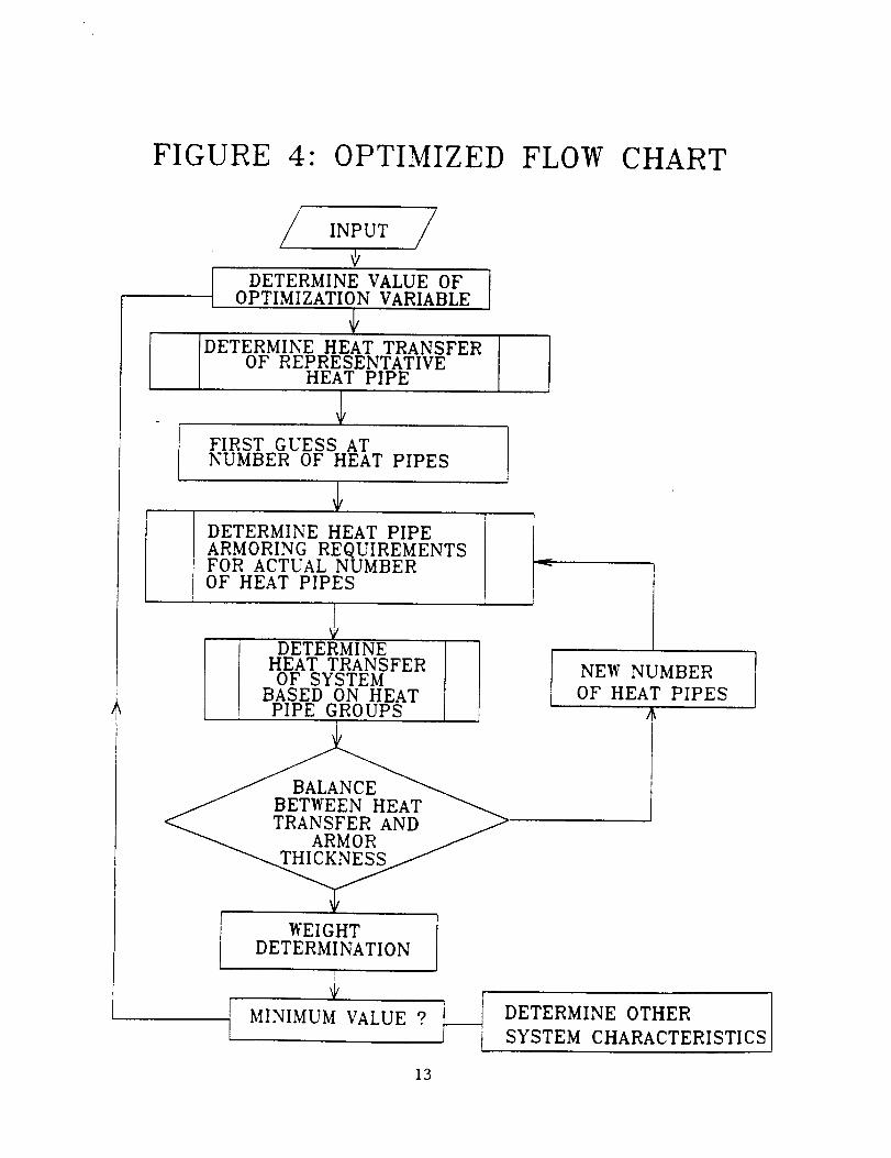
FIGURE 4: OPTIMIZED FLOW CHART
" INPUT /
DETERMINE VALUE OFOPTIMIZATION VARIABLE
I OF REPRESENTATIVEI HEAT PIPE
I FIRST GUESS ATNUMBER OF HEAT PIPES
DETERMINE HEAT PIPEARMORING REQUIREMENTSFOR ACTUAL NUMBEROF HEAT PIPES
HEAT TRANSFEROF SYSTEM
BASED ON HEATPIPE GROUPS
WEIGHTDETERMINATION
NEW NUMBER
OF HEAT PIPES
A
t
I MINIMUM VALUE ? DETERMINE OTHER
SYSTEM CHARACTERISTICS
13

heat pipe can dissipate is determined. This calculation is done assuming the
heat pipe has no protective armor. The value calculated is used to estimate
the total number of heat pipes required for the entire radiator section. If
the temperature and temperature change required in the radiator design
requires more than one type of heat pipe working fluid, then the switch-off
point (location where a different heat pipe fluid is used) is determined.
This allows the determination of the required heat transfer of each group of
heat pipes in a radiator section. The same procedure as outlined above is
used for determining an initial guess for the required number of each heat
pipe type to meet the specifications in the radiator section.
Once an initial guess for the number of all the heat pipe types is
obtained, redundancy is included, and a total area is determined for the
radiator section. This area is used along with the requirements on misslon
life, system altitude, redundancy, and required probability of radiatorsurvival to determine the armor thickness for the heat pipes. At this point,
a suitable estimate exists about the radiator section to begin the detailed
analysis. A new value for the number of heat pipes is determined accountingfor the armor thickness. At this time, an estimate of the required size of
the transport duct is determined based on the number of heat pipes required.
With this information, an estimate is made of the required armor thickness on
the transport duct. This is based on the user specified transport duct design
(i.e. location of the heat pipes in relation to the transport duct), duct
material specifications, redundancy, and required survivability. When the
armor thickness is determined, it is used to calculate a thermal resistance.
With this known, an estimate of the transport duct heat transfer is calculated
based on the average duct fluid temperature in the radiator section. This
value is used to adjust the number of heat pipes required in the system. The
iteration process with the heat pipes starts again and continues until the
final design is converged upon for total number of heat pipes and transportduct size.
2.1.4.2 OPTIMIZED APPROACH
The basic approach used for the analysis with the optimizing approach is
not significantly different than that described above for the basic analysis.
Several differences do exist though.
To be able to do the calculations for the radiator design numerous times
for the mass minimization, groups of heat pipes are used instead of single
ones to determine heat transfer capabilities. The total temperature drop of
the radiator pumped loop fluid is broken into increments of approximately 5 K.
Allowances are made when switch-off points between different heat working
fluids are used. The required heat transfer of the fluid within this
increment (i.e. product of mass flow, specific heat, and temperature change of
the fluid) is determined. The arithmetic average temperature of the fluid
within one of these increments is used as the temperature at the outside of
the heat pipe evaporator. The heat transfer capabilities of a single heat
pipe at that average temperature is calculated. The total number of heat
pipes for the increment is determined by multiplying the ratio of total
required heat transfer in the increment to that obtained for a single heat
14

pipe. This process continues for the entire radiator temperature drop and all
heat pipe fluids. The mass of this radiator design is then calculated in the
same way as is done for the non-optimizing approach.
The optimized design approach requires the user to choose upper and lower
limits for the variable that is changed during the mass minimizing process
(e.g. a minimum and maximum redundancy value must be specified when this is
chosen as the optimizing variable). The system mass is initially determined
for the specified upper and lower values as well as for the mid-point
optimizing variable value. Brent's optimizing method determines the final
variable value to give a minimized system design. This method uses the slope
of system mass lines to determine the next variable guess for minimizing the
system mass (see Reference 17 for additional information on this numerical
method).
The technique used for minimizing the radiator system mass only allows
one variable to be varled at a time. Therefore, when more than one heat pipe
working fluid is required, the optimizing variable of only one heat pipe type
is used to determine a minimum mass system. When this calculation is
completed, the variable relating to the next heat pipe type is optimized to
calculate the new system mass. This continues until all the different heat
pipes types have been optimized for the specified variable and the final
result reflects the overall system minimum mass.
It is not desirable to have the optimizing algorithm terminated due to a
self imposed error in the program (refer to section 4.3), therefore, certain
flags and conditions are set internal to the program during the analysis. Any
situation which produces an error condition during the normal analysis will
trigger a flag in the optimization run that establishes a high, artificial
value of the system mass for that design point. The variable causing the
error condition is eliminated from the analysis. This continues until a
optimizing variable range is established that is with the program geometrical
constraints. Therefore, even though the user may specify the optimized
radiator to be established within a wide range of variable values, the program
may reduce this range to one that can be addressed by the limitations of the
code. In the output, the user is able to follow the events of the program to
tell what has happened during calculations with out-of-bounds conditions.
This method has worked a majority of the time, however, several instances have
been found in which the optimization has not progressed correctly using this
procedure. Therefore, it is recommended that when an error condition is
triggered (indicated by an estimated mass of the system of 1E8 kilograms in
the output), the user should rerun the analysis with a smaller specified range
for the optimization variable.
2.___22 GEOMETRY POSSIBILITIES
The radiator configuration can be varied substantially. The only basic
constraint is that the design is one in which a fluid is transported to the
evaporative sections of heat pipes. Various geometries can be designed via
the use of the two view factors prescribed for the radiator system. Anything
from flat plates, to cylinders, to cones, to a spoked wheel design, as well as
15
others, can be modeled with the use of independent view factors for two sides
of the radiator. A user must spend some preliminary design effort todetermine the correct values for the two view factors.
Within any geometry, the actual radiator operation can be accomplished in
many ways. As mentioned previously, redundancy can be used for both the heat
pipes and the transport ducts. Therefore, any number of independent transport
ducts can be specified in a design, with any number of these belng required to
survive the entire mission. Attached to these ducts are the heat pipes that
can also be redundant. These redundant heat pipes will simply increase the
basic size of the transport.
The value of the heat pipe redundancy is expressed as a percentage of the
number of heat pipes required for successful system operation at the end of
mission. For instance, if it is determined that 100 heat pipes are required
to reject the heat in a radiator section, and 8Z redundancy is specified,
there will actually be 108 heat pipes present in the final design. Due to the
random nature involved in a failure from Particle impacts, redundancy is used
for all the heat pipes with different working fluids. Therefore, the same
relative amount of extra heat pipes will be present for all the different
working fluids.
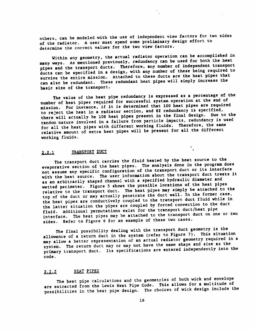
2.2.1 TRANSPORT DUCT
The transport duct carries the fluid heated by the heat source to the
evaporative section of the heat pipes. The analysis done in the program does
not assume any specific configuration of the transport duct or its interface
with the heat source. The user information about the transport duct treats it
as an arbitrarily shaped channel with a specified hydraulic diameter and
wetted perimeter. Figure 5 shows the possible locatlons of the heat pipes
relative to the transport duct. The heat pipes may simply be attached to the
top of the duct or may actually penetrate the duct wall. In the former case,
the heat pipes are conductively coupled to the transport duct fluid while in
the latter situation the pipes are coupled by forced convection to the duct
fluid. Additional permutations exist for the transport duct_heat pipe
interface. The heat pipes may be attached to the transport duct on one or two
sides. Refer to Figure 6 for an example of these two cases.
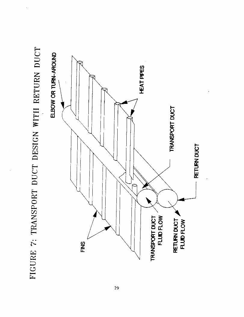
The final possibility dealing with the transport duct geometry is the
allowance of a return duct in the system (refer to Figure 7). This situation
may allow a better representation of an actual radiator geometry required in a
system. The return duct may or may not have the same shape and size as the
primary transport duct. Its specifications are entered independently into thecode.
2.2.2 HEAT PIPES
The heat pipe calculations and the geometries of both wick and envelope
are extracted from the Lewis Heat Pipe Code. This allows for a multitude of
possibilities in the heat pipe design. The choices of wick design include the
16
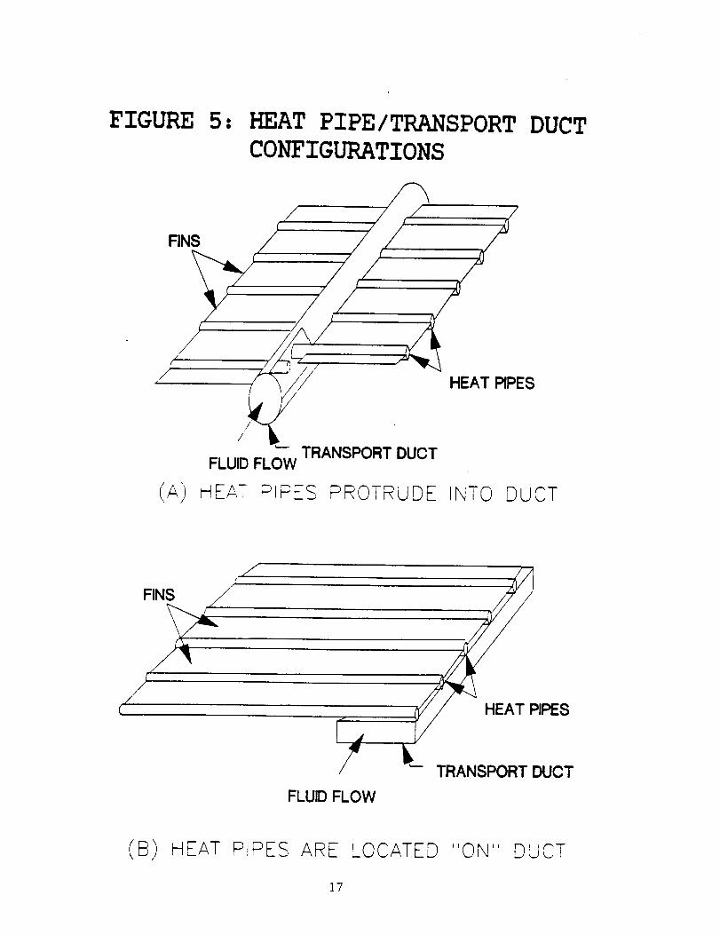
FIGURE 5" HEAT PIPE/TRANSPORT
CONFIGURATIONS
DUCT
FINS
/
HEAT RPES
(A)FLUID FLOW
TRANSPORT DUCT
HEAT PIPES PROTRUDE INTO DUCT
FINS /_
,/
// HEAT PIPES
" • Y
TRANSPORT DUCT
FLUID FLOW
(B) HEAT PIPES ARE LOCATED "ON" DUCT
17
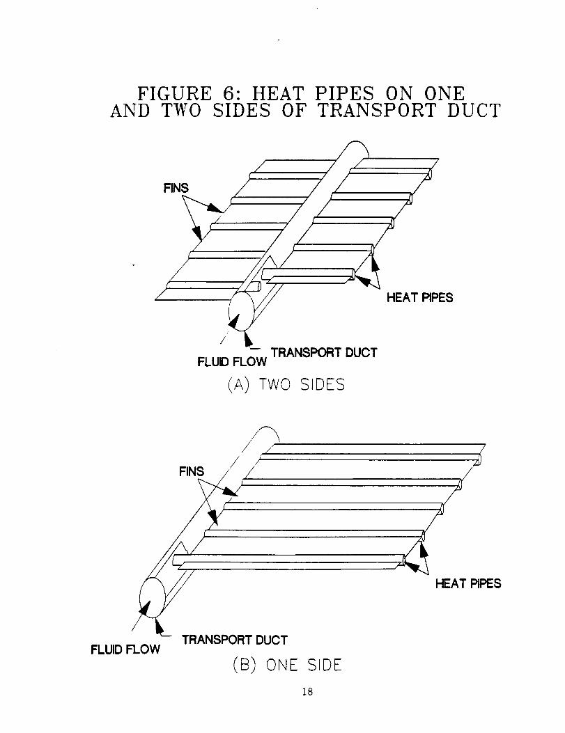
FIGURE 6: HEAT PIPES ON ONEAND TWO SIDES OF TRANSPORT DUCT
HEAT PIPES
/
/
-- TRANSPORT DUCTFLUID FLOW
(A) TWO SIDES
/j j;
FI l/
/
TRANSPORT DUCTFLUID FLOW
(B) ONE SIDE
HEAT PIPES
18
E.-
0
Z
A:
\
I
_z \J _ I_ '_l"lr"I-.
19

use of axial grooves, wire mesh screens, with or without arteries, sintered
metal wicks, also with or without arteries, and a generic wick in which the
user specifies all the geometric and hydrodynamic aspects of the wick
structure. The basic assumed shape analyzed for the heat pipe envelope is a
cylinder, however, specifying certain variables can result in the modeling of
non-circular envelopes for the heat pipe cross section. The details of the
requirements to describe non-circular heat pipes are described in Section 3.2.
Also specified by the user are the heat pipe entrainment number, wetting angle
of the fluid/envelope combination, and the nucleation radius available on the
heat pipe envelope surface. These factors are also described in more detall
in the user input sections of this manual.
2.3 MATERIALS
A built-ln materials library is featured in the code. It is comprised ofa substantial number of materials that have been considered for use in
radiator systems. The choices available are described below with any
applicable comments effecting their use.
2.3.1 FLUIDS
2.3.1.1 TRANSPORT DUCT
The transport duct fluids available for use in the code are shown in
Table 3. The code number for the fluid is used to identify it in the program
input and output.
Table 3 : Transport Duct Fluids
Fluid Code Number
Lithium 1
NaK 2
Helium 3
Toluene 4
Sodium 5
Potassium 6
Cesium 7
Water 8
Mercury 9Methanol i0
Freon-ll 11
Heptane 12Dowtherm A 13
Ammonia 14
User specified properties 15
When the user input option is chosen, the program requires thermodynamic
20

information of the fluid that is to be used in the calculations. The
information needed is specific heat, density, thermal conductivity, and
viscosity. Temperature dependent properties are not available for use.
Therefore, if a user specified fluid is to operate over a large temperature
range, and its properties vary considerably over this range, the results
obtained for the analysis may not be as accurate as desired. This must be
kept in mind during a design. The program is easily expanded to include more
working fluids, which is planned, however, those listed above constitute the
current limits of the program.
2.3.1.2 HEAT PIPE
Available heat pipe duct fluids are shown in Table 4. Included in the
fluid list are the associated numbers that identify the fluid in the input and
output of the program as well as the suggested applicable temperature ranges
(taken from Reference 10). It should be noted that no user properties can be
entered for heat pipes. This is because the properties have to be entered as
temperature dependent values due to the way in which the heat pipe performance
is calculated. As with the transport duct fluid, the basic program can be
modified to add additional fluids as information becomes available.
Table 4 : Heat _ Fluids
Fluid Code Number
Potassium 1
Lithium 2
Sodium 3
Cesium 4
Water 5
Mercury 6
Methanol 7
Freon-ll 8
Heptane 9
Dowtherm A 10
Ammonia ii
Applicable Temperature Ran_e
773 K to 1273 K
1273 K to 2073 K
873 K to 1473 K
723 K to 1173 K
303 K to 473 K
523 K to 923 K
283 K to 403 K
233 K to 393 K
273 K to 423 K
423 K to 668 K
213 K to 373 K
2.5.2 METALS
2.3.2.1 LINERS/ARMORS/FINS/WICKS
The metals currently available for use in the code for liners (the use of
liners for heat pipes and transport ducts is discussed in Section 2.3.2.4),
armoring material, and fins ere shown in Table 5. The associated reference
number that is used to identify them in the program output and input is also
shown. All of these materials may be used for the transport duct, heat pipes
including the wicks, or fins. Any of them may be used as a liner or armoring
21

material in the system design, however, it should be noted that the metals
with an asterisk do not have known armor property capabilities. Their impact
coefficient will be determined by the following equation:
K z - 0.92/(p/1000.) °'5 with p - density in kg/m 3
K_ is the impact coefficient for the NASA Thin Model - refer tosection 2.5.2 of this manual for detailed discussion of the
mathematics of the calculations for impacts.
This equation is a curve fit of impact coefficients for materials with known
armoring capabilities. It is assumed to be applicable to other ductile
materials, however, the use of the materials with unknown armoring properties
should be carefully scrutinized when used in a radiator design.
Table 5 : Materials for Liners, Armor. Fins. and Wicks
Metal Code Number
Stainless steel 1
Titanium 2
Beryllium 3Aluminum 4
Magnesium lithium 5Niobium-i zirconium 5
User properties 7Iron** 8
Nickel** 9
Copper** I0
Tungsten** iiInconel** 12
Molybdenum** 13
Tantalum** 14
Indicates that armoring property capabilities are currently
unknown, and their impact coefficients are determined by the above
equation. This aspect of the analysis has not yet been changed in
the program, and currently, the use of these materials do not
provide any armoring protection.
The user specified properties option allows the incorporation of any
material for use in the program. This, therefore, allows the incorporation of
such things as composite materials for use in a radiator design. The
properties required for system design include density and thermal
conductivity. The armoring capabilities of a user defined material is
calculated in the same manner as that for the materials with unknown
protection capabilities. As with the user defined fluid properties, a
temperature dependence of the user defined materials is planned, but not
22
currently available. Therefore, the same warning exists for materials that
have very temperature dependent properties used in a system that experiences a
large temperature change.
2.3.2.2 BUMPERS
As of yet, no calculations are included in the code to allow for use of
offset bumpers in the determination of armoring requirements. Input exists in
the program for the use of bumpers, but the information is not used. 0nly
basic armoring calculations are assumed to occur.
2.3.2.3 COMPATIBILITY INFORMATION
Much experimental work has been done with heat pipes, and it has been
determined that not all heat pipe working fluids and heat pipe envelope
materials are compatible with one another. Two materials may produce an
interaction that causes the heat pipe to fail. A listing of known
compatibilities (acceptable and adverse) is contained in Reference ii. This
information has been included in the HEPSPARC code. Based on the material
choices, information is provided in the code output to indicate known
compatibility information between the heat pipe fluid and its wick and
envelope material. Even though the transport duct and transport fluid do not
behave in the same manner as the heat pipe, compatibility information is also
provided for the duct system to alert the designer of any known history
regarding the materials chosen for the overall design.
2.3.2.4 LINERS
A material is chosen for a heat pipe or transport duct system to provide
maximum armoring capabilities. However, often this material is not compatible
with the fluid it must contain. In such a case, a liner may be employed in
the system (refer to Figure 8). This provides a material barrier between the
fluid and outside material. It allows the use of the best armoring materials
with the best heat pipe fluids even though they may be incompatible. The
liner material will also offer some armoring capabilities.
This code allows for the design of transport duct system and heat pipes
with the liner material. Even though the user may specify a particular
combination of armor, liner, and fluid, it still may not be manufacturable.
Nothing is contained in the code to estimate the compatibility between the
armor and liner material. Several things are recommended to the designer to
evaluate this aspect. One is to examine the coefficients of thermal expansion
of the two materials and the stress that would be induced in them for the
radiator design. If one of the materials will yield, the use of the material
combination may be questionable. An additional area to check is the
possibility of a chemical interaction between the liner and armor material.
23

2_

2.3 •2.5 PROPERTIES
The material properties used for the analysis in this program can be
obtained from a source listing of the code (refer to section 5.0 of this
manual). The data was taken from a combination of places. Much of the
material information was taken directly from the NASA Lewis Heat Pipe Code
(Reference 9). Additional data was the result of material property curve fits
obtained from various literature sources (Reference 12). The impact data was
obtained from a NASA report on the subject (Reference 8).
2.__/_ HEAT TRANSFER DETAILS
2.4.1 OVERVIEW
This section of the manual discusses in detail the methods employed to
determine the heat transfer that occurs from the radiator system. It is meant
to provide sufficient information and references to allow the interested user
to follow the program calculations and structure.
The basic method employed for the code has already been described. The
program heat transfer calculations operate in the same manner for both the
optimization and non-optimized version of the code. The thermal resistance of
various sections of the design are determined and the temperature drop through
these resistances is calculated along with the heat transfer from the
particular section of interest. The heat transfer calculated is equated to
the temperature drop experienced by the transport duct fluid. At this point,
the next heat pipe, sections of heat pipes or transport ducts are addressed in
the calculations. The code progresses through the radiator system until the
overall design requirements have been met (i.e. the transport duct fluid has
met is specified temperature change). This entire process includes the
armoring methodology described elsewhere in this manual.
2.4.2 TRANSPORT DUCT FLUID
2.4.2.1 BASIC EQUATIONS
The heat transfer coefficient to determine the temperature drop from the
transport duct fluid to either a heat pipe immersed in the fluid or to the
duct wall itself is determined by standard empirical relationships. The
different areas and fluids in the transport duct require several different
correlations for the total range of applicability of the program. The
equations used in the program are described below.
Flow across a heat pipe evaporator: Heat transfer from fluid to a
cylinder;
Liquid metals:
= (k/Dout,£d, of b,at pip,)[5.0 + 0.025(ReDPr) 0.s ]
25
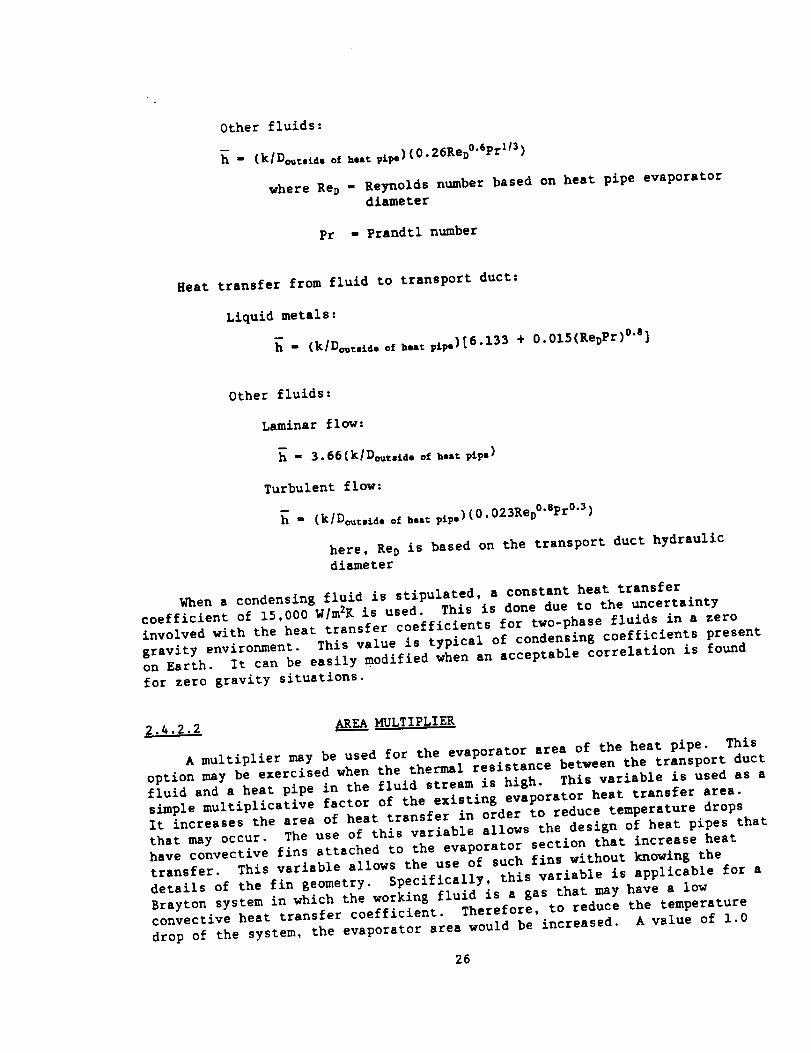
Other fluids:
" (k/D_,td. of h..t p£_)(0"26Rev °'6Prll3)
where Re D = Reynolds number based on heat pipe evaporatordiameter
Pr - Prandtl number
Heat transfer from fluid to transport duct:
Liquid metals:
" (k/D_t,lde of h,at pt_)[ 6-155 + 0-OIS(ReDPr) O'a]
Other fluids:
Laminar flow:
= 3.66(k/D_t,lde of heat pi_)
Turbulent flow:
h - (k/D_t,tde of heat pip,)(O'O23ReD O'sPr°'3)
here, Re D is based on the transport duct hydraulicdiameter
When a condensing fluid is stipulated, a constant heat transfer
coefficient of 15,000 W/m2K is used. This is done due to the uncertainty
involved with the heat transfer coefficients for two-phase fluids in a zero
gravity environment. This value is typical of condensing coefficients present
on Earth. It can be easily modified when an acceptable correlation is found
for zero gravity situations.
2.4.2.2 JL_EAMULTIPLIER
A multiplier may be used for the evaporator area of the heat pipe. This
option may be exercised when the thermal resistance between the transport duct
fluid and a heat pipe in the fluid stream is high. This variable is used as a
simple multiplicative factor of the existing evaporator heat transfer area.
It increases the area of heat transfer in order to reduce temperature drops
that may occur. The use of this variable allows the design of heat pipes that
have convective fins attached to the evaporator section that increase heat
transfer. This variable allows the use of such fins without knowing the
details of the fin geometry. Specifically, this variable is applicable for a
Brayton system in which the working fluid is a gas that may have a low
convective heat transfer coefficient. Therefore, to reduce the temperature
drop of the system, the evaporator area would be increased. A value of 1.0
26

for this variable will allow an analysis to proceed with the basic heat
envelope determining the heat transfer area.
2.4.3 HEAT PIPE
In situations in which more than one heat pipe fluid is required for a
system, the switch-over point between fluids is governed by the recommended
upper bounds of the lower operating temperature heat pipe fluid. This allows
a radiator to be designed for an end of life operating condition in which
specified final system requirements are stipulated. Such a configuration
exists when all redundant heat pipes have been destroyed, and the radiator is
just able to meet the system heat transfer requirements. In the transport
duct, non-operational (redundant) heat pipes exist upstream heat pipe fluid
switch-over points. At these points, the lower temperature heat pipe fluid
will have to operate at its maximum temperature. Therefore, by specifying the
a switch from a higher temperature heat pipe fluid to a lower one to occur at
as high a temperature as possible, end of mission requirements will be able to
be met without much possibility of the heat pipes operating beyond one of
their thermal or hydraulic limits. Before the radiator reaches this end of
mission configuration, the transport duct fluid at the switch-over points will
be at a lower temperature and will require the heat pipe will simply operate
further into its recommended intended design range.
2.4.3.1 EVAPORATOR/CONDENSER
The heat pipe heat transfer is calculated in the same manner as is done
in the NASA Lewis Heat Pipe Code (Reference 9) and therefore, the specific
equations will not be furnished here. It is done via the use of a heat
transfer resistive network that accounts for all sections of the heat pipe.
The heat pipe model uses three separate nodes; one in the evaporative section
and the remaining two in the condenser. The network contains all the elements
that exist to retard heat transfer from the outside of the evaporator wall to
the outside of the condenser wall (see Figure 9). The resistances that are
taken into account during the analysis of the heat pipe are the resistance
through the outside armor and liner wall in the evaporator, the wick thermal
resistance, the resistance across the liquid vapor interface in the
evaporator, and the resistance through the vapor itself down to the condenser
section of the heat pipe. In the condenser the resistance network is just
reversed from that in the evaporator, i.e. across the vapor/llquid interface,
through the condenser wick structure, and then through the liner and armor in
the condenser. The resistances for the condenser section is done at two
separate nodes to account for the possibility of a large temperature drop
through the heat pipe at near thermal-hydraulic limit conditions.
2.4.4 FIN.____SS
The heat transfer from the radiator occurs due to radiation interchange
from the outside surfaces to the space environment. The heat pipes are
assumed to have conducting fins located between adjacent pipes. These are
27

@
28
v0
0
rrrr _.-OrrOo
w(D
b_rr
used in radiator design to help reduce the mass of the system. The fins
decrease in temperature alon E their length due to the heat loss from their
surface. Typically, the effectiveness of the fin is expressed as a fin
efficiency. This is the ratio of amount of heat a fin actually transfers to
the amount of heat that could be transferred from a same sized isothermal
surface at the temperature of the fin base. Due to the fln/heat pipe
configuration, not all of the heat radiated from the surface will be directed
towards the space sink (see Figure 10). Some of the energy that emanates from
the heat pipe will be intercepted by the fin or adjacent heat pipes, and
thereby reducing the effectiveness of the heat pipe surface. The fin will
also radiate energy that is intercepted by the heat pipes. This phenomenon is
accounted for in the code. An analysis was done to determine the effects of
geometry on the fin and surface efficiencies. The description and results of
that analysis are presented below.
2.4.4.1 GRAY BODYANALYSIS
The procedure for determination of surface and fin efficiencies is
outlined in Reference 13 and was performed on the basic configuratlon shown in
Figure i0. The surfaces were assumed to be gray, i.e. they were not assumed
to be perfect emitters and absorbers. The analysis broke the configuration
down into differential sized elements. View factors were determined between
all elements, and an iterative scheme was developed to determine the
radiosities of the differential elements. From that, the total heat
transferred from the surfaces was determined. This analysis was done for
various combinations of fin length, thickness, pipe size, and surface
emissivities. Additionally, the analysis allowed adjacent heat pipes to be
operating at slightly different temperatures which may actually be the case in
a radiator. The heat transfer values calculated were then compared to a gray,
flat, isothermal surface of the same size to establish the effectiveness of
the heat pipe, via a surface efficiency, and the fin, via a fin efficiency.
These values are used in the code in a manner described in the following
section.
2.4.4.2 TABULATED DATA
The results of the gray body analysis has been entered into HEPSPARC by
means of a simple look-up table. Geometrical factors, temperatures, thermal
conductivity, and surface emissivity values are all used to determine the
appropriate table location in which to obtain surface and fin efficiencies. A
factor to account for the effect of non-isothermal adjacent heat pipes is also
in tabulated form, and is used as a multiplicative adjustment to the
efficiency values.
The total heat transfer that occurs from the outside of the heat pipe
surface ks calculated from the data obtained An the table as:
Q " ½(F1+F2)_(T4surface " T4,ink)(_eurfaceAheat pipe + _finAfin )
with FI or 2 " view factor of side 1 or 2 of the radiator to
29

pm.q
T_
30
Tsink
G • Stefan-Boltzman constant
heat pipe and sink temperatures
adjusted surface and fin efficiencies
respectively. These already account for
non-isothermal adjacent heat pipes and a
specified emissivity to be present on the
surfaces. That is why E does not appear
in the above equation.
Ahear pipe .Afin m Total heat pipe and fin surface areasrespectively
One desired modification to the program will be to allow different
emissivities on the fins and heat pipes. Current restrictions allow only one
emissivity to be specified for all of the radiator surfaces. This does not
necessarily represent a condition that would actually exist when radiator
design uses different fin and base materials.
2.__.55 ARMOR DETAILS
The methodology employed for the determination of armor thickness of the
radiator surface, specifically the heat pipes and transport ducts, isdescribed in this section.
2.5.1 FLOW' CHAR.____T
The basic flow chart of the calculation of the armor thickness is shown
in Figure ii. The details involved in the process, including all the
supporting equations are presented below. The process requires an iterativemethod of solution to determine the armor thickness of the radiator.
2.5.2 BASIC ARMORING EQUATIONS AND METHODS
The method followed for a determination of the armor requirement is taken
directly from Reference 6 and is simply synopsized here for completeness of
this document. Several modifications were made to the basic approach outlined
by Fraas to tailor the calculations to the situations being analyzed. They
will be pointed out as required. If the reader is unfamiliar with basic
armoring methodology, it is reco_nended that Reference 6 be reviewed prior to
trying to understand this section.
Micro-meteoroids:
Particle distribution models exist that describe the level of certain
31

FIGURE 11: DETAILED ARMORING CALCULATION
INPUT /
FIRST GUESS ATNUMBER OF HEAT PIPES
(NO ARMORING)
DETERMINE HEAT PIPE
ARMORING REQUIREMENTS
ACCOUNTING FORREDUNDANCY
DETERMINE
HEAT TRANSFER
RESISTANCEDUE TO ARMOR
DETERMINE NEW
TEMPERATURE DROP
THROUGH ARMOR
CALCULATE TOTALNUMBER OF HEAT PIPES
NEW NUMBER
OF HEAT PIPES
ARMOR
CALCULATIONS
DONE
32

mass particles present in the space environment. For micro-meteorolds, the
near earth flux has been modeled as:
logloN t - -14.37 -l.21oglom
with N t - average meteoroid flux (number of particles, of mass equal
to or greater than m grams, per m2-s)
This expression can be corrected for the defocusing effects of the
earth's gravitational field by multiplying by:
G, - 0.568 + 0.4321R (R - (6578+H)16378 H - orbital altitude in km)
and
E = (i + cos@)/2 with 8 • arcsin[6378/(6378 + H)]
The thickness of a given material for incipient penetration by an
impacting particle has been estimated as:
t - K,mp°'_bpp °'17v°'88
where
t = material thickness, cm
K I- penetration constant of given material
mp= mass of particle, g
pp= density of particle, g/cm 3
V = particle velocity, km/s
This is the NASA thin Plate model. The equation can be solved to determine
the mass of a particle required to penetrate a given material thickness. This
is substituted into the flux equation to determine the flux of particles (Nil)
having mass equal to or greater than the mass required to penetrate the
material thickness for the given velocity (V£). Combining all the above
yields:
Nti= 4.27 x 10 "15 G,Et'3"_bKI3"45#p0"58V0 "31
This flux corresponds to a particular velocity increment. In order to obtain
the total value of the flux, the particle velocity profile is broken apart and
the probability of each velocity is then used to determine an overall lethal
flux value (Nit).
Nlt = _ Nti Pi where Pi " probability of velocity V i occurring for
the micro-meteoroids
When this is done for the micro-meteoroid distribution, the following
expression results:
Nit - 7.15 x i0 "n G,Et'3"_bK1S'_bpp 0"$8
The particle density,pp, is assumed to be 0.5 glcm 3.
33

The probability of impact of an exposed radiator area by n or fewer lethal
particles during a mission ks described by a Poisson distribution:
rsn
P (h<__)" exp (-NI_AT ) Z (NI_AT )r]r 1r-0
where
P {h(n) m
N1 t m,
A
T
probability of impact by n or fewer lethal particles. This
corresponds to the probability of survival of the radiator
heat pipes or transport duct systems.
lethal particle flux, partlcles[m2-s
exposed radiator area to be protected, m 2
mission duration, seconds
An iterative technique is used to determine the values in the above
equation. The required area is determined from the heat transfer calculations
(in the heat pipe case), or from the assumed design (for the transport ducts).The redundancy of the system is used to increase this area. The number of
redundant components represents the value of n in the above equations. For agiven thickness, redundancy, altitude, and material, the probability of n
number of lethal impacts is determined. This probability is then compared to
the desired system probability of survival. The thickness it adjusted and the
calculation repeated until the correct probability is determined. Thethickness calculated is used to redetermine the system heat transfer.
Debris:
Space debris is addressed An the same way as the micro-meteoroids. Thetotal lethal flux for debris is determined to be:
Nit - 8.89 x 10"10t'2"22K12'22Od 0"37
In this case, the debris density, Pd, is assumed to be that of aluminum,
or 2.7 g/cm 3. Also note that there is no correction for earth defocusin E or
system altitude. This level of flux is taken as the value estimated to be
present for year 2020.
If the radiator exposed areas were the same for the micro-meteoroids and
debris, the two fluxes calculated above would simply be added to give a grand
total flux for use in the Poisson expression and in the determination of the
material thickness iteration scheme. However, different areas may exist for
the use with the two fluxes. The areas used, and their justification is
described in Section 2.5.5.
Space debris and micro-meteoroid fluxes have a definite directional
nature to them that may be calculated. Specific orbital information related
to the spacecraft is required. However, this program is not capable of such
specific analysis, and the directional aspects are not included. The flux
levels presented are for a worst case situation to produce a conservative
34

design.
2.5.3 BASIC BUMPERING METHODOLOGY
Bumpering refers to the use of armor that is not directly adjacent to the
structure being protected. A certain distance exists between the bumper and
underlying surface. The concept behind bumpering is that the use of the
bumper will cause impacting particles to either be vaporized due to impact
with the bumper or to be broken apart. The resulting fragments will be of a
lower mass and be dispersed over the underlying surface. This surface may be
thinner than if it were exposed to the normal distribution of particles since
the particles reaching it have a lower mass, and therefore, a lower lethal
particle flux.
The method used to determine the effectiveness of the bumper is given in
Reference 8, however, as mentioned before, this is currently unavailable as
part of the code calculations. This section was added to make the user of the
code aware of the need and desire to include this armoring aspect in an
improved version of the radiator code.
2.5.4 USE OF MULTI-LAYER MATERIALS
In designs in which more than one type of material is used for the armor
surface (e.g. using a liner material on heat pipes), the relationship
specified between lethal particle flux and thickness may be conservative.
Therefore, an alternative calculational method has been established. Whereas
the equations determined above were for the thickness of material at incipient
penetration (NASA Thin Plate Model), when a multi-layer material is used, the
required thickness may be reduced (Reference 14).
The analysis is based on the model of an impact of a particle with a
semi-infinite body (NASA Thick Plate Model). The basic equation relating these
is (Reference 6):
P® = K.mO.35pmo.17vO.67
where P® - depth of penetration, cm
K, = material constant
m = mass of micro-meteoroid, g/cm 3.
Pm = micro-meteoroid density. Use a value of 0.5 as before.
V - impact velocity
A correction factor (CF) to this depth of penetration is then applied to
determine the wall thickness when a multi-layer material is used for a thinwalled structure.
t - CFxP®
The analysis proceeds as before to determine the lethal flux for the
micro-meteoroid distribution. It is determined to be:
35
Nit - 5.79 x 10 "12 G,Et-3'45CF3"4_X.3"45pp°'Ss
For this equation, the particle density,pp, is again assumed to be0.5 s/cm _.
The correction factor used may have any value. A value of 1.5 has been
used previously in the SP-100 analysis [Reference 14), and therefore, it isthe only choice currently available.
The same procedure used above may be followed for the space debris flux to
give_
Nit - 2.69 x 10 "10 t'2"22CF2"22K.2"22pd°'37
Again, the grand total of these two fluxes will be used in the Poisson
distribution calculation from above. These are the equations used for lethalflux determination in the iteration calculations when a correction factor is
specified.
The material thicknesses determined from all the above calculations (NASA
Thin and Thick Plate models) are used to determine the actual required armor
thickness to account for the presence of any liner on the section being
analyzed. The thickness (t) of a liner is converted into an equivalent armor
thickness by use of the following relationship_
tRquivalant a_or " Kl,a_ortZ_lr/Kl,liner
where the K1 values are the impact coefficients for thearmor and liner materials for the NASA Thin Model
This equivalent thickness is subtracted from the calculated required thicknessvalue to determine the actual armor thickness.
2.5.5 VULNERABLE AREAS
The area used in the determination of the exposed area for the armoring
calculations may be varied somewhat. The flux of micro-meteorolds is
considered to be isotropic in nature, and therefore, a lethal particle may
arrive from any direction. Therefore, the total exposed area of the heat
pipes and transport duct is required to be used for determining the armoring
requirements for micro-meteoroids. In the case of a heat pipe, the exposed
area is the circumferential area of the pipe.
The area to be used for space debris may be different. It is unknown
whether debris behaves isotropically or in a more planar manner suggested by
some (Reference 15). In the former case, the total area would have to be
used, but in the latter, a projected area would constitute the exposed
surface. In that case, the diameter of a heat pipe (multiplied by the exposed
length) is used for the determination of armor for the space debris flux.
36
All the areas used are corrected for the configuration of the radiator
design. The heat transfer view factor of the two "sides _ of the radiator
surface is used to reduce the exposed area. This is done to compensate for
the fact that a radiator design may help shield itself. For instance, a
cylindrically shaped radiator will obviously not have the same probability of
impact on its interior surface as it does on its outside. Therefore, it is
assumed that the same view factor exists to the debris and micro-meteorold
source that exists for the surfaces to the specified heat sink temperature.
Additionally, for the transport duct, some additional shielding will occur if
a return duct is added to the system. This shielding will reduce the exposed
area of the duct. The amount of the shielding will be determined by the
specific configuration of the duct design. Since it would be very difflcult
to attempt to determine all the data required to calculate the amount of
shielding that occurs when a return duct is used in a system, it has been
assumed that 75Z of the total surface area of a round or non-round transport
will be exposed to the space environment fluxes of debris and micro-meteoroids
when a return duct is used and the total surface area is used for armor
determination. When a projected area is assumed for use with the micro-
meteoroids, only half of this value of vulnerable area (37.5/) is used for
armor determination on the transport duct. These values were determined to be
present on specific designs HEPSPARC was used with. It is believed to be a
good estimate of the vulnerable area present when a return duct is used. If
the user does not feel that it correctly models a particular design, it may
easily be changed within the program.
2.6 OTHER DETAILS
This section details other features of the code. This includes pressure
drops and other details of the transport duct fluid as well as details
concerning stress levels calculated in the code.
2.6.1 PRESSURE DROP
The pressure drop experienced by the fluid in the transport duct is
estimated in the program. This allows for the determination of pumping power
(see below) so a designer may estimate this aspect of the radiator system.
The pressure drop and pumping power will detract from the overall system
performance and will have to be supplied by some system power source.
The pressure drop in the system is dependent on the frictional energy
loss the fluid undergoes while moving through the transport duct. The code
breaks the calculation down into several different sections for analysis.
When the heat pipes do not project into the transport duct, the total pressure
drop is determined by the basic duct flow equation:
AP - 4pV2fL/(2D) where V - fluid velocity
f - friction factor (see below)
L - length of duct
D - hydraulic diameter of duct
p = density of fluid in transport duct
37

The equations used for friction factor vary in the above analysis with respect
to the Reynolds number of the flow. They are determined as follows:
For Reynolds number (Re) < 5000
f - 16/Re
and for 5000 _ Re _ 30,000
f - 0.079Re -o.25
and for Re E 30,000
f - 0.046Re -0.20
When the heat pipes project into the duct, the Reynolds number used is
dependent upon the area being examined. Areas required to be examined include
the entrance and exit of the radiator panels, the area in between heat pipes,and the area directly adjacent to the heat pipes. A Reynolds number is
determined for each of these sections and the corresponding friction factor
determined. Each of the pressure drops associated with these areas is
determined and added to estimate the overall pressure drop expected in the
entire system. The pressure drop for the total number of panels determines
the value for each independent radiator loop.
The friction characteristics for the pressure drop determination were taken
from Reference 16. Although the correlations are specifically for round
pipes, the use of the hydraulic diameter should give reasonable estimates of
the friction factor for the pressure drop calculations for non-round transportducts.
The pressure drop due to heat pipes being in the duct is accounted for by
determining the pressure drop over a single tube in cross-flow. It is
realized that this is not the best way to model the situation due to possible
effects from the proximity of the transport duct. Some type of single, in-
line tube bank correlation may be better, but none was found for incorporation
into the code. It is estimated that the use of the single tube in cross-flow
will produce conservative results. Tube banks typically have a lower pressure
drop due to a shielding effect from upstream tubes.
Loss coefficients can be added to the system pressure drop to account for
the presence of elbows, restrictions, and other actual duct possibilities.
The way in which they are used is to multiply the loss coefficients and the
velocity head of the transport duct fluid to obtain the additional system
pressure drop. No use of the equivalent diameter method is employed.
2.6.2 PUMP NORK
Pump work is estimated based on the calculated system pressure drop.
is the volume flow rate of fluid (Q) multiplied by the pressure drop:
It
38

Pumpwork = QAP= m_P/p with m • mass flow rate of fluid in transportduct
p • density of fluid in transport duct
AP• system pressure drop
This estimates the power required for a 1001 efficient pump to move the fluid
through the radiator system as designed. Actual requirements will depend on
any additional pumping requirements present in the loop as well as the
hydraulic and electrical efficiency of the pump and motor combination chosenfor use.
2.6.3 STRESS ANALYSIS
The hoop stresses in heat pipes and transport ducts are estimated in the
program. Even though the transport duct, and at times the heat pipes, may not
be circular in shape, the stress determined in a cylinder is used to estimate
the effect of pressure in the system.
Hoop stress: a = Pr/t with P • pressure of fluid in transport duct
or heat pipe
r • radius of heat pipe (based on
diameter of heat pipe used for armor
determination) or hydraulic diameter
of transport duct divided by 2
t • thickness of wall of transport duct
or heat pipe (includes liner and
armor thickness)
39
3.__O0 USER INPU____T
3.__.!1 INTRODUCTION
This section is used to provide a line by line description of the how thecode is used. Both the interactive and non-interactive input characteristics
will be explained.
The non-interactive method will be addressed initially. The procedure
that wlll be followed will be to show the actual lines of data required for
the program. The meaning of each variable will be explained as well as any
applicable variables or flags that may be set or triggered within the program
by a given response. This will help in the description of the interactive use
of the program. All combinations of responses will be addressed for both the
optimization and non-optimized use of the code. The questions as they appear
from the code will appear in bold faced text as will the lines of data that
are created in the input file.
3.__! INTERACTIVE ANDNON-INTERACTIVE|4ETHODS
3.2.1 NON-INT,ERACTIVE USE
This section describes the actual physical make-up of the input file.
This file can be created manually, but the interactive use of the program wlll
also accomplish the task in an error free manner. The details in this section
will allow the user to easily modify a file created during interactive usage
of the program, or actually create a file from scratch. It is recommended
that the interactive method be used at least for the initial description of a
radiator design to ensure the data has been input correctly. In this section
an input file line (shown in bold face) will be expressed with the appropriate
variable names, then the options, values, and ramification of certain choices
will be described as they relate to the variables. This will serve two
purposes. First, it will compliment the information provided below concerning
the "walk through" of the program. Second, it wlll furnish a list of
variables that are actually used in the code for calculational and logic
purposes. This will aid a user in the determination of the logic involved in
many of the algorithms. Two additional things need to be specified. The code
uses an unformatted read statement of the input file, therefore, the user does
not have to worry about ensuring that certain variables are located in
specific columns of the file. The input information must be separated by a
comma or a space. Secondly, the code uses an implicit specification for
integers and real valued variables. Therefore, any variable beginning with
the letters I through N (inclusive) are considered to be integers and must be
entered into the input file as such. These variables generally constitute
counters and flags within the program structure.
NOPT,NPAN,PWID,IPANT,DIH,HPEEIM,ICOND,M,COEF
NOPT - Optimization flag variable. NOPT = 0 for non-optimized use of code
while NOPT - i is to use the algorithm in a mass optimization
40

ll'_nner.
NPAN - Number of radiator panels per independent transport duct path.
PWID - Maximum total radiator panel width in meters. Can only be used
when NOPT-0. Occurs when a fixed transport duct width will be
specified for the radiator (IDES=l; explained below) and this
value will be used to determine the heat pipe condenser length.
This value will depend on if the heat pipes are specified to
emanate from one or two sides of the transport duct.
IPANT - Type of radiator panel. IPANT-I: heat pipes project from only one
side of the transport duct; IPANT-2: heat pipes project from both
sides of the transport duct.
DIH - Primary transport duct effective hydraulic diameter in meters. It
is determined from the following equation:
DIH - 4A c/P. where Ac - duct cross-sectional area
P, - duct wetted perimeter
HPERIM - Wetted perimeter of primary transport duct in meters.
ICOND - Fluid phase flag. If ICOND - 0: transport duct fluid is single
phase (i.e. all liquid or all gas); ICOND - i: two-phase fluid is
used in the transport duct. Currently, when this option is
exercised, a heat transfer coefficient of 15,000 W/m2K is used for
the condensing vapor. This is due to the fact that a zero-gravity
correlation condensing correlation is unknown to the author.
M _ Number of different heat pipe types used in the radiator. A heat
pipe type is defined as one in which the working fluid is
different. The code is intended to allow the use of several (up
to 5) different heat pipe working fluids within on radiator system
in order to allow a large transport duct fluid temperature change.
C0EF - Loss coefficient of an independent transport duct network (non-
dimensional) for supplemental pressure drop determination.
If the optimization routine is used (NOPT-I), the following lines follow in
the input data set:
NVAR
NVAR - This variable indicates which variable is to be used for the mass
optimization. The available choices are:
NVAR - i;
NVAR = 2;
NVAR - 3;
NVAR - 4;
Fin thickness
Fin width (defined as the distance between outside
diameter of heat pipes)
Heat pipe redundancy
Heat pipe diameter
41

NVAR = 5; Variation of number of independent transport ducts
surviving the entire mission duration
If NVAR = 1, the next lines in the input file will be:
TFINHI,TFINLO
These are the upper (TFINHI) and lower (TFINL0) constraints of the fin
thickness (in meters) for the optimization. The algorithm will only
determine a minimum mass system that has the optimization variablebetween these values. The line is repeated M (as defined above) times
to account for all the different heat pipe types. The variable order is
from the highest temperature heat pipe working fluid to the lowest.
If NVAR - 2, then the next lines will appear:
Fk'IDHI,I_/IDLO
These are the upper (FWIDHI) and lower (FWIDLO) constraints for the fin
width (in meters). As with the fin thickness, the line is repeated M
times starting with the high temperature heat pipe conditions.
If NVAR = 3, then the following will appear:
RZDHI,LEDLO
These are the upper (REDHI) and lower (EEDLO) constraints of the heat
pipe redundancy. It is assumed that all the different heat pipe types
will have the same relative amount of redundancy. The values that are
to be entered are calculated as follows:
RED - 1.0 + Eedundancy (in percent)/100.
Therefore, a 5 percent redundancy constraint would be specified by a
1.05 value entered into the input file.
If NVAR - 4, the followin E is specified:
DBI,DLO
These are the upper (DHI) and lower (DL0) constraints of the actual heat
pipe diameter in meters. As with the other parameters, it is repeated M
times account for the different heat pipe types. It starts with the
high temperature pipe and continues to the low.
If NVAR - 5, no additional constraints need be specified. The number of
surviving independent transport ducts is automatically varied from i up to the
maximum number possible. The mass results for all the possible values will
appear in the output file.
After the lines for the optimization case (if they are required), the
42

following will appear:
HL,ENI.,T,KXLT,IHLM,HLT,ICONV,LHPLOC
Ht- Maximum radiator duct length per panel, in meters. To be used
when NOPT=0. Occurs when a fixed transport duct length will be
specified for the radiator (IDES=l; explained below) and this
length will be used to determine the heat pipe spacing. The inlet
and outlet lengths of the transport duct are subtracted from this
length for each panel, and the heat pipes are then evenly
distributed over the remaining duct length. If the IDE$-I option
is not exercised, the required transport duct length will be
determined for the system based on specified fin width values.
ENLT - Entrance length of transport duct for each radiator panel that
contains no heat pipes (in meters).
EXLT - Exit length of transport duct for each radiator panel that
contains no heat pipes (in meters). The entry and exit lengths of
the transport ducts may represent portions of a radiator that are
required for some other use such as a deployment mechanism.
IHLM - Transport duct liner material code flag. See 2.3.2.1 for the
associated material flag values. If no liner is to be used, any
integer value may be entered.
HLT - Transport duct liner material thickness in meters. When no liner
is used, a value of 0.0 should be specified for the variable.
ICONV - Flag that specifies the boundary condition on the external
radiator surface. ICONV = 0: represents a condition of pure
radiative heat transfer from the outside surface; ICONV-I: a
combined convective and radiative heat transfer system exists on
the radiator surfaces.
LHPLOC - Flag that specifies the relative location of the heat pipes on the
transport duct. LHPLOC-I: the heat pipes protrude into the
transport duct and come into physical contact with the duct fluid;
LHPLOC=2: the heat pipe is located on the transport duct and is
coupled to the duct fluid by conduction through the duct and heat
pipe wall. This latter arrangement is the one present on the SP-
i00 radiator configuration.
If ICONV = I, the next line will appear:
HCONV
This is the external convective heat transfer coefficient that is
present on the radiator external surfaces.
IHAR,IHWF,AQ,TIN,TOUT,IDES,NPARA,NLOSS,NPAN
43
IHAE - Transport duct material code flag. See section 2.3.2.1 for theactual material associated with each variable value.
IH_F - Transport duct working fluid code flag. Section 2.3.1.1 describes
the fluids and their codes available for use in the program.
Desired heat transfer of the radiator at the end of llfe condition
in kilowatts.
TIN - Inlet temperature of the transport duct fluid in K.
TOUT - Desired outlet temperature of the transport duct fluid in K.
IDES - Flag that specifies how a radiator design will be developed. This
option is not available when the optimization method of analysis
is chosen (i.e. NOPT - 2) and the IDES flag should then be set to
be equal to 2. When the non-optimized version of the code is
used, this variable may be set to equal to i. When this is the
case, it is assumed that severe constraints are to be placed upon
the maximum size of the radiator structure. Therefore, both a
maximum transport duct length (per panel) and maximum radiator
panel width is assumed to be required in the design. These
stipulations then allow the program to determine certain variable
values that would normally be specified as input by the user when
this option is not used. Specifically, the heat pipe condenser
length is calculated as the specified panel width (PWlD) minus the
transport duct diameter. This length would be divided by two if
the heat pipes project from both sides of the transport duct.
Also, the fin width is determined by subtracting the outside
diameters of all the system heat pipes and the lengths of the
inlet and outlet sections of the transport ducts from the total
transport duct length (accounting for all the radiator panels) and
dividing this value by the total number of heat pipes required in
the system. Thus, it is assumed the heat pipes and fin will take
up all the available duct area. If IDES is set to equal 2, both
the fin width and heat pipe condenser length must be specified by
the user for each heat pipe type. When _DES-1, all the different
heat pipe types will be assumed to have the same condenser length.
This may create some out of limit conditions for the heat pipes.
The use of the IDES-1 option does have some applications in a
design situation, but it is recommended that the program be used
with the IDES variable set to equal 2.
NPARA - Number of independent parallel transport duct paths in the
radiator at the beginning of the m/ssion.
NLOSS - Number of allowable inoperative (due to mlcro-meteoroid and space
debris impact punctures) transport ducts at the end-of-mlssion
configuration.
NPAN - Number of sections or panels of radiator per each independent
parallel path.
44

If the transport duct fluid was specified to have user defined properties,
i.e. an IHWF of 15, the following line will next appear in the input datafile:
CPHF,CONDHF,VISCHF,EHOHL
CPHF - Specific heat of the transport duct fluid in J/kgK.
CONDHF - Thermal conductivity of the transport duct fluid in W/mE.
VISCHF - Viscosity of the transport duct fluid in N-s/m 2.
RHOHL - Density of the transport duct fluid in kglm _.
The following line will then occur either after the NPAN or RBOHL value:
RPR,TSINK,F1,F2,I_iIS,FLOW, ITRANS
RPR - Inlet pressure of the transport duct fluid in the radiator. It is
used to determine the pressure stresses of the transport duct.
TSINK - Effective sink temperature the radiator panels experience. To
yield a conservatively sized radiator design, this variable should
be the maximum value that will be experienced during a mission oran orbit.
F1 - Effective view factor of side number 1 of the radiator to the
effective sink temperature. For the radiator being designed, if
the heat pipes are located on (versus in) a transport duct, the
two sides of the radiator will not be symmetrical. If this is the
case, side 1 is defined as the side of the radiator panel having
the transport duct located on it. It should be noted, when the
heat pipes are located in the transport duct, this distinction is
not applicable.
F2 - View factor of side 2 of the radiator to the effective sink
temperature. This, alon E with the F1 variable allow for the
design of a radiator in nearly any geometry.
EMIS - The emissivity of the external surfaces of the radiator. All the
material that comprises the radiator is assumed to have the same
emissivity.
FLOW - This variable represents the mass flow rate of fluid through the
entire transport duct system (i.e. all independent paths) at the
beginning of the radiator mission life. This only applies when
the fluid in the transport duct is specified as being condensed,
(ICOND = i). If the fluid in the transport duct is single phase,
the FLOW variable should be entered as zero. The flow rate is
specified in kg/s of fluid. The heat transfer of the system is
45
then determined by:
ITRANS -
Q - mhfs
m - mass flow
hfg - enthalpy of vaporization
This variable specifies whether a return transport duct is
included in the radiator system design. If one is to be included,
ITRANS - 1 is specified, while ITRANS - 0 assumes no return duct
is present in the design. If one is included, a certain amount of
it will have to be protected with armoring or bumpering. The main
and return ducts are assumed to be located adjacent to one another
in the system design. Therefore, they will tend to shield each
other from micro-meteorolds and space debris. The actual amount
of shlelding depends on the shapes of the return and main
transport duct. A value of 251 shielding has been assumed for
ducts of circular and non-circular cross sections. Therefore, 751
of the total combined area of the normal and return duct are used
for the vulnerable area calculation. This is for the assumption
of total vulnerable area available for space debris exposure.
When a projected area is assumed for this calculation, only half
of this value of vulnerable area is used for armor determination
on the transport duct for the mlcro-meteoroid fl_x.
If a return duct is specified for the system (ITRANS - 1), then the following
should be entered on the next data line:
RETDIH, RETPER
RETDIH - Return transport duct hydraulic diameter in meters.
RETPER - Return transport duct wetted perimeter in meters.
The followin E line will appear after either the data for the return transport
duct or after the line ending with the ZTRANS variable.
SURVHP, SURVTD, RED,ALT, IENV, DURR, ADWPP ,ADSW
SURVHP -
SURVTD -
This specifies the required survivability of the heat pipes in the
system. This value is used in the determination of the armor
thickness of the heat pipe. A typical value would be .95 to
represent a 95Z probability of the heat pipes survivability.
This specifies the required survivability of the transport duct(s)
in the radiator system. This value is used in the determination
of the armor thickness of the ducts. The variable is specified in
the same way as the SURVHP variable. The product of the heat pipe
and transport duct survivabilities will yield an overall system
survivability value.
46
RED -
ALT -
IENV -
DURR -
ADWPP -
ADSW -
This variable specifies the redundancy to be used for the heat
pipes. This variable is also used in the determination of the
heat pipe armor thickness. The value entered is determined in the
same way the REDHI and REDLO are determined, i.e. a RED value of
1.05 signifies a 5Z desired redundancy. It should be noted that
for this variable, as well as any other variable that can be
optimized, may have any value in the main data deck when it has
been chosen for use in the optimization. When the optimizing
option is used, the controlling variable are the limits specified
for the optimization specified in the third line of the input
deck.
This is the altitude in kilometers at which the radiator is to
operate during its mission. This value helps determine the micro-
meteoroid flux that will be experienced during a mission.
This variable specifies the environment for the radiator system.
If IENV - 1, then only micro-meteoroids are assumed to be present,
and the radiator armoring thickness will be calculated based only
on this flux. If IENV - 2, space debris will also be considered
to be present in the radiator environment.
This represents the desired mission life of the system in years.
This variable is used to add weight to the system. It represents
the additional mass (in kg) to be added in the system analysis for
each radiator panel present in the entire system. This may be
indicative of some structural mass requirement for each panel such
as a deployment mechanism required for each panel.
This variable is also used to account for additional masses
.present in the system that may not be covered by this analysis.
This variable represents the extra, lump sum, mass (in kilograms)
to be added for the entire radiator system.
ADWPS,NARN,NAREA,AHPHTD,N/4OD,AHULT
ADWPS - This variable is also used to add mass to the system. It
represents the additional mass (in kilograms) to be added during
the analysis for each independent section of the radiator. It may
represent, for example, the mass of a pump that would be required
for each independent transport duct.
NARM- This variable represents the choice of armoring design for the
transport duct. If NARM - i, then normal armoring methods are
used, while NARM = 2 specifies that offset bumpering techniques be
employed. Currently, no bumpering calculations exist, and
therefore, NARM should always be specified to be equal to I.
NAREA - This flag represents the vulnerable area determination to be used
in the armor determination for space debris protection. A NAREA
47

AMPMTD-
NMOD -
AMULT -
value of 1 signifies the actual circumferential area is to he used
while a NAREA of 2 indicates the projected surface area will be
used in determining the vulnerable area of the heat pipes or
transport duct. This option was added due to the uncertainty
involved in the nature of space debris.
This variable also adds mass to the system analysis. It
represents the addition of mass (in kilograms) for each meter of
transport duct length for each transport duct. It may represent
some type of mass adjustment, such as a bumper, for the entire,
unknown transport duct length.
This variable is used to specify the model to be used for thearmor determination. If NMOD - I, the NASA Thin model will be
used, while NMOD - 2 indicates the NASA Thick model with a
correction factor will be used. Section 2.5.2 of this manual
discusses the details of these two models.
If the NASA Thick model is used, the AMULT variable specifies the
correction factor to be used with it. Currently, the NASA Thickmodel calculations have a built-ln correction value of 1.5.
Therefore, the specification of AMULT does not affect it. This
will be changed in the future. The recommended range of this
value will be 1.5 to 2.5. If the NASA Thin plate model is
specified (NMOD-1), then this variable should be set to be zero.
If the material chosen for the transport duct liner is to be user specified
(IHLM -7), the next line will follow.
CONHLM,RHOHLM,HLK1
CONHLM - Transport duct liner material thermal conductivity (W/mE).
RHOHLM - Transport duct liner material density (kg/m3).
HLKI - Transport duct liner material impact coefficient (as would be used
with the NASA Thin plate model).
If the material chosen for the transport duct armor is to be user specified
(IHAM -7), the next line will follow.
CONHAM,RHOHAM,HAK1
CONHAM - Transport duct armor material thermal conductivity (W/mE).
RHOHAM - Transport duct armor material density (kg/m3).
HAKI - Transport duct armor material impact coefficient (as would be used
with the NASA Thin plate model).
48

The final lines in the program describe the details of the heat pipes to be
used in the radiator design. Therefore, there will be M sets of the following
data starting with the highest temperature working fluid heat pipe.
EVAP,DHPA,HPLTE,HPLTC,IHPF,IHPL,IHPA,1WT,FINT,PACTO&
EVAP - This variable ks the length (in meters) of the evaporator section
of the heat pipe. This ks the length of the pipe either in or on
the transport duct depending upon the design.
DHPA - This variable represents the actual heat pipe diameter (in meters)
(assuming the heat pipe is round). This value is used to
determine the vulnerable area of the heat pipe. An equivalent
diameter can be determined for non-round heat pipe designs.
HPLTE - This variable represents the specified thickness (in meters) of
the liner material in the evaporator region of the heat pipe. If
no liner is to be used, then this value should be set equal to
zero.
HPLTC - This variable represents the specified thickness (in meters) of
the liner material in the condenser region of the heat pipe. If
no liner is to be used, then this value should be set equal to
zero.
IHPF - This variable specifies the fluid used in the particular heat
pipe. Section 2.3.1.2 of this manual indicates the fluids
available for use and their applicable temperature ranges. The
first heat pipe (and fluid) specified should be able to be used at
the radiator inlet temperature. If the fluid can not cover the
entire temperature range required for the radiator, additional
heat pipes and fluids will have to be specified in the input deck.
IHPL - This flag specifies the liner material choice for the heat pipe.Section 2.5.2.1 indicates the choices available for the materials.
If no liner is to be used, this should be set equal to be zero.
IHPA - This flag specifies the armor material choice for the heat pipe.
Section 2.3.2.1 indicates the choices available for the materials.
IWT -- This variable identifies the wick design for the heat pipe. The
following choices are available:
IWT - 1 - Rectangular grooves
IWT - 2 - Screen wick
IWT = 1 - Sintered metal wick
IWT - 1 - Generic wick described by user properties
IWT - i - Screen wick with arteries
IWT - I - Sintered metal wick with arteries
FINT - This is the thickness (in meters) of the fin attached to the heat
pipe. If the fin thickness is to be optimized, then this variable
49
should be set equal to zero.
FACTOR - This variable represents a multiplicative factor to be used on the
available heat transfer area on the heat pipe evaporator section.
This allows for adding augmentation to the outside of the heat
pipe evaporator (which would come into contact with the transport
duct fluld). It may be used in such a case when a gas with a low
heat transfer coefficient is being used as the transport duct
medium. Then, fin materlal may be desired to be added to the
external evaporator area in order to reduce this thermal
resistance. If no augmentation is desired, a value of one should
be specified for FACTOR.
IWM,DHP,IFIN
IWM -- This variable specifies the wlck materlal flag. Section 2.3.2.1
indicates the material associated with the various values of INM.
DHP - This variable specifies the diameter (in meters) of the heat pipe
that will be used for the thermal/hydraulic calculatlons. For
round heat pipes, this will have the same value as the DHPA
variable, but for non-round designs, they may be substantiallydifferent.
IFIN - This flag specifies the material to be used for the fins. Section2.3.2.1 indicates the available choices of material.
If the IDES variable is equal to two (by user choice or by default when
running an optimization design), the following line will next appear in thedata deck.
FINW,HPCL
FINW - This variable is the fin width (in meters). Fin width is defined
to be the distance between adjacent heat pipes (i.e. outside
surface to outside surface).
HPCL - This variable represents the heat pipe condenser length (in
meters).
If the heat pipe liner material is to be of a user specified material, (IHPL -
7), then the following line is required.
CONDL,HFRHOL,HPLK1
CONDL - Heat pipe liner material thermal conductivity (WlmK).
HPRHOL - Heat pipe liner material density (kg/m_).
HPLKI - Heat pipe liner material impact coefficient (as would be used with
the NASA Thin plate model).
50
If the heat pipe armor material is to be of a user specified material, (IHPA -
7), then the following line is required.
CONDA,HPRHOA,HPAK1
CONDA - Heat pipe armor material thermal conductivity (W/mX).
HPRHOA - Heat pipe armor material density (kg/m3).
HPAKI - Heat pipe armor material impact coefficient (as would be used with
the NASA Thin plate model).
If the fin material is to be of from user specified properties (IFIN -7), the
following line will have to appear:
CONDF,RHOFIN
CONDF - Heat pipe fin material thermal conductivity (W/mK).
RHOFIN - Heat pipe fin material density (kg/m3).
The following lines describe the wick details for the particular heat pipe
design. Additional details about the required inputs can be obtained from the
authors of Reference 9. This section of the code was taken directly from that
work.
If IWT - 1 (Rectangular Groove), one line is required to describe the wick:
DEEP. WII_RV, NUM
DEEP - Depth of the rectangular grooves (in meters).
WIDGRV - Width of the rectangular grooves (in meters).
Number of rectangular grooves around the periphery of the heat
pipe. Note, the number and size of grooves can not exceed the
available circumference length (i.e. NUM x WIDGRV < = x (DHP -
2(DEEP))).
If IWT - 2 (Screen Wick), one line is required to describe the wick:
DIAM,WIDE,CRIMP,NDMWRP
DIAM -
WIDE -
CRIMP -
Screen wick wire diameter (in meters).
Center to center spacing between wick wires (in meters).
Crimping factor of screen wire wick.
51

_P - Number of wraps of screen specified for the wick design.
If IWT = 3 (Sintered Metal), one line is also required for the data:
TWICK.PORW,RSS
TWZCK - Thickness of the sintered metal wick (in meters).
PORW - Porosity of the wick structure. A PORW value of 0.50 indicates a
50Z porous wick structure.
Average radius of the sintered particles which comprise the wick
structure (in meters).
RSS -
If IWT - 4 (User Input Wick Properties) then five lines of data are required:
AKE,AKC,PE
AKE -
AKC -
This variable represents the product of the evaporator wick
permeability and the wick area (m4).
This variable represents the product of the condenser wick
permeability and the wick area (m4).
PE - This is the value of the inner perimeter of the heat pipe An the
evaporator section (for thermal/hydraulic calculations not for
armor determination) in meters.
PORE,PORC.AKEE
PORE - This variable is the porosity of the wick structure An the heat
pipe evaporator section. It should be entered into the data deck
in decimal form (i.e. 0,50 - 50Z porosity).
PORC - This variable is the porosity of the wick structure An the heat
pipe condenser section. It should be entered into the data deck
in decimal form (i.e. 0,50 - 50Z porosity).
AKEE - This represents the evaporator effective wick thermal conductivity
(Wlm z K).
A]EEC,AVE,AVC
AKEC - This represents the effective wick thermal conductivity in the
condenser section of the heat pipe (W/m 2 K).
AVE - This is the effective vapor area available in the heat pipe
evaporator section (in m2).
52

AVC - This is the effective vapor area available in the heat pipecondenser section (in m2).
RCM,DCRITE,RATAR
ECM - This variable is the maxlmummeniscus radius available in the heat
pipe wick structure (in meters).
DCRITE - This is the value of the critical entrainment dimension in the
heat pipe evaporator wick (in meters).
RATAE - This variable represents the ratio of the inside area of the
evaporator to its open area.
AREAWE, AREAWC
AREWE - This represents the actual cross sectional area of the wick
structure in the evaporator of the heat pipe. It, alon 8 with the
porosity are used to determine the mass of the wick in the heat
pipe evaporator reaion.
AREAWC - This represents the actual cross sectional area of the wick
structure in the condenser section of the heat pipe. It, alon 8
with the porosity are used to determine the mass of the wick in
the heat pipe condenser section.
When IWT - 5 (Screen wick with arteries), two lines of data are required.
first is the same required for the screen wick alone:
DIAM,WlDE,CRIMP,_WRP
The second line describes the arteries:
EA,AWT,NA
RA-
AWT -
NA -
Radius of arteries in the wick (in meters).
Thickness of the artery wall (in meters).
Number of arteries in the wick structure.
The
If IWT - 6 (Sintered Metal wick with arteries), two lines of data are also
required. The first one is the same as the slntered metal wick:
TWICK,PORW,RSS
The second line describes the arteries:
53

RA,WICCON, HA
RA -- Radius of arteries in the wick (in meters).
WICCON - Thermal conductivity experimental constant. For metal or felt
fiber, a WICCON value of 0.34 should be specified. If sintered
partlcles.are used, a value of 0.53 is to be specified.
NA - Number of arteries in the wick structure.
The final line required for the heat pipe definition is then:
RN.THETA.WEBNUM
RN - Minimum nucleation radius of heat pipe envelope material (in
meters). A suggested value of this variable is lxlO "6 meters.
THETA - This represents the wetting angle between the heat pipe fluid and
wick material (in degrees).
NEBNUM - This represents the Weber number at the onset of entrainment for
the particular heat pipe.
This completes the data required for analyzing or designing a radiator. If
additional heat pipes are required for the design, the data on the line
starting with the EVAP variable would next be entered. The data would
continue until the heat pipe fluid is capable of operating at the radiator
outlet temperature.
3.2.2 INTERACTIVE USAGE
This section describes the questions that are used to query the user for
a response during interactive use of the program. Even though it is highly
reconnnended that this approach be used (at least initially) to create the data
file for an analysis, it was decided to first describe the actual data deck
that is required for the program before the actual interactive details are
provided (refer to section 3.2.1). This section is meant to compliment the
previous one. The actual questions that appear during the use of the program
will appear in bold faced type. Then, the variable being triggered by the
response will be identified as will any results of the particular variable
choice. The description of the variables discussed can be obtained fromsection 3.2.1.
Both the optimized and non-optimized version of the code as well as their
usage and interactive input requirements will be addressed in this section.
The optimized approach will be addressed initially.
54

IS THEDATAFORTHISRUNCIIKKENTLYIN ANEXISTING DATA FILE ? (Y/N)
Answering "N" to this question automatically invokes the
interactive usage of the code. By responding with a "Y", the
program then asks for the data file name, and then proceeds to use
that file for the analysis.
OPTIMIZATION CHOICES: (ENTER 1 OR 2)
1. MINIMUM MASS 0PTIKIZATION RUN
2. UNOPTIMIZED, SIMPLE MASS DETERMINATION RUN
ENTER i or 2:
Variable triggered - NOPT
If optimization is chosen the following will appear:
DESIRED SYST_PAEAMETER TO BE VARIED:
1. FIN THICKNESS
2. FIN WIDTH
3. SYSTEM REDUNDANCY
4. HEAT PIPE DIAMETER(S)
5. NUMBER OF PANELS SURVIVING
ENTER CHOICE:
Variable triggered - NVAR
SYSTEM PARAMETERS:
TOTAL HEAT_ECTIONREQUIRED (kW):
Variable triggered - AQ
RADIATOR INLET T_fPEEATUEE (K)_
Variable triggered - TIN
RADIATOR OUTLET T_fPERATURE (K):
Variable triggered - TOUT
RADIATOR INLET PRESSURE (kPa):
(FOR STRESS CALCULATION PURPOSES)
Variable triggered - RPR
IS CONDENSATION PRESENT IN THE TRANSPORT DUCT (Y/N) ?
Variable triggered - ICOND
If condensation is present, the following will appear:
55

TOTAL SYST_4MASS FLOW RATE OF CONDENSING FLUID AVAILABLE (kg/s):[i.e. BEGINNING OF LIYE)
Variable triggered - FLOW
SINK TDIPERATURE (K):
Variable trissered - TSINK
VIEW FACTOE OF SIDE i TO SINKs
MOTE: SIDE 1 IS DEFINED AS THE SIDE WITH THE TEANSPOETDUCTWHEIq THE
HEAT PIPES ARE ON, NOT IN, THE DUCT
I_qTERVALUE
Variable trigsered - F1
VIEW F&CTOR OF SIDE 2 TO SINK:
Variable trissered - F2
I_fISSIVITY OF EXTERNAL SUEFACES:
Variable triggered - EMIS
SURVIVABILITY INFORMATION:
HEAT PIPE SUEVIVABILITY PROBABILITY (Z):
Variable trissered - SUEVHP
Note - in the interactive case, a percent value is entered.
TRANSPOET DUCT SURVIVABILITY PROBABILITY (Z)z
Variable triggered - SURVTD
If redundancy is to be optimized, the followin 8 will appear:
LOWER BOUND FOE EEDUNDANCY IN ANALYSIS (Z):
Variable trisEered - REDLO
UPPER BOUND FOR REDUNDANCY IN ANALYSIS (Z):
Variable trisEered - REDHI
If redundancy is not to be optimized, the followin S will appear instead:
PERCENT REDUNDANCY DESIRED:
Variable trissered - RED
Note - this is entered in percent also.
EARTH ORBIT ALTITUDE (km):
56

Variable triggered - ALT
ENVIRONMENT:
i. MICRO-METEOROIDS
2. MICRO-METEOROIDS AND SPACE DEBRIS
ENTER CH01CE:
Variable triggered - IENV
MISSION DURATION (YEARS):
Variable triggered - DURR
PENETRATION MODEL TO USE:
1. NASA THIN MODEL
2. NASA THICK MODELWITHANADJUSTMENT FACTOR
ENTER CHOICE:
Variable triggered - NMOD
If the NASA Thick model is chosen, the next line will appear:
DESIEED MULTIPLICATIVE FACTOR (RECOP_ENDED RANGE 1.5 TO 2.5):
Variable triggered - AMULT
AREA USED TO _TE _LEAREA FOR SPACE DEBRIS IMPACT:
1. ACTUAL, CIRCUMFERENTIAL AREA
2. PROJECTED AREA
ENTER CHOICE:
Variable triggered - NAREA
IS THERE CONVECTION ON THE RADIATOR EXTERNAL SURFACES (YIN) ?
Variable triggered - ICONV
If there is to be convection, the following line will appear:
ENTER CONVECTIVE HEAT TRANSFER COEFFICIENT (W/m**2 K)
Variable triggered - HCONV
TRANSPORT DUCT INFORMATION:
TYPE OF TRANSPORT DUCT:
I. HEAT PIPES PROJECT TO ONLY ONE SIDE
2. HEAT PIPES PROJECT IN TWO DIRECTIONS
ENTER 1 or 2:
Variable triggered - IPANT
57

TRANSPORT DUCTJHEAT PIPE CONFIGURATION:
1. HEAT PIPE PROTRUDES INTO TRANSPORT DUCT
2. HEAT PIPE IS LOCATED OH TRANSPORT DUCTENTER 1 or 2:
Variable triggered - LHPLOC
IS THERE TO BE A RETURNDUCT ON THE TEANSPOETDUCT (YIN) 7
Variable triggered - ITRANS
TRANSPORT DUCT PROTECTION SCHI_4E:
1. NORMAL ARMOEING PROCEDURES2. OFFSET BIR4PERING IS TO BE USED
ENTEECHOICE:
Variable triggered - NARMNote - only choice #I is currently allowed
TOTAL NUMBER OF PARALLEL PATHS:
Variable triggered - NPARA
If the number of transport ducts surviving is not to be opti_/zed, the
following line will appear.
NOMBEROFALLOWABLE PATH LOSSES
Variable triggered - NLOSS
TRANSPORT DUCT(S) EFFECTIVE HYDRAULIC DIAMETER (m)z
Variable triggered - DIH
TRANSPORT DUCT WETTED PERIMETER (m):
Variable triggered - HPERIM
If a return duct is to be used in the analysis, the following two lines will
appear:
RETURN TRANSPO&T DUCT(S) EFFECTIVE HYDRAULIC DIAMETER (m):
Variable triggered - RETDIH
RETURN TRANSPORT DUCT WETTED PERIMETER (m):
Variable triggered - RETPER
ESTIMATE OF TRANSPO&T DUCT(S) LOSS COEFFICIENTS (PER PANEL):
Variable triggered - COEF
58

PANELINFORMATION:
NUMBER OF PANELS IN EADIATOR (PER PARALLEL TRANSPORT DUCT PATH):
Variable triggered - NPAN
If the non-optimized version of the code is being used, the following line
will appear:
1. DESIGN OF RADIATOR TO BE BASED ON COMPUTER GENERATED TUBE SPACING
(i.e. FIXED TRANSPORT DUCT LENGTH w_ NO OPTIMIZATION)
2. USER SPECIFIED FIN WlDTH
Variable triggered - IDES
If IDES - 1 is specified, the following two lines will appear:
MAXIMUM PANELWIDTH (m):
(TO BE USED TO DETERMINE CONDENSER LENGTH)
Variable triggered - PWID
MAXIMUM TRANSPORT DUCT LENGTH PER PANEL (m):
Variable triggered - HL
INLET LENGTH OF TRANSPORT DUCT(S) (m):
Variable triggered - ENLT
OUTLET LENGTH OF TRANSPORT DUCT(S) (m):
Variable triggered - EXLT
TRANSPORT DUCT LINER THICKNESS (m):
Variable triggered - HLT
If there is to be a liner, the following will appear:
TRANSPORT DUCT LINER MATERIAL:
NOTE: CHOICES 8 THROUGH 14 WILL OFFER NO S_GTH FOR MICRO-METEOROID_
DEBRIS PROTECTION IN CALCULATIONS
A list of material choices will then appear. The user should respond by
entering the number of the material chosen.
Variable triggered - IHLM
If the material choice is the user specified material, the following three
lines will appear:
59
THERMALCONDUCTIVITY(W_mK):
Variable trisgered - CONHLM
DENSITY (kglm3):
Variable triEgered - R/4OHLM
THRESHOLD PENETRATION CONSTANT:
Varlable trIKsered - HLK1
TRANSPORT DUCT ARMORIBUMPEIMATEIIALz
A list of materials will then appear. The user should respond by enterin 8 thenumber of the material chosen.
Variable triggered - IHAR
If the material choice is the user specified material, the following three
lines will appear:
THERMAL CONDUCTIVITY (W_mK):
Variable trigsered - CONHAM
DENSITY (kE_m3):
Variable trisgered - EHOHAM
THRESHOLD PENETRATION CONSTANT:
Variable trigsered - HALKI
TRANSPORT DUCT WORKING FLUID:
A list of fluid choices will then appear.
Variable tri88ered - IHWF
If the fluid choice is the user specified material, the followin E four lines
will appear:
DENSITY (kglm3) :
Variable triEsered - RHOHL
THERMAL CONDUCTIVITY (WlmK):
Variable triEsered - CONDHF
FLUID VISCOSITY (Ns_m**2):
60
Variable triggered - VISCHF
FLUID SPECIFIC HEAT (Jlkg):
Variable triggered - CPHF
HEAT PIPE INFORMATION:
At this point, all the heat pipe information is going to be determined.
Initially, a menu will appear indicating the available fluids that may be used
for the heat pipes in the temperature range of interest. Also appearing will
be the range of temperature over which the various heat pipe fluids are
applicable. For example, if the inlet temperature of the transport duct is
850 K, the following menu will appear:
1. POTASSIUM
4. CESIUM
6. MERCURY
(RANGE 773 K TO 1273 K)
(RANGE 723 K TO 1173 K)
(RANGE 523 K TO 923 K)
The user should specify the fluid choice by entering the number of the desired
fluid, e.g. enter 4 for cesium.
Variable triggered - IHPF
If the heat pipe diameter is to be optimized during the analysis, the
following two lines will appear:
LOWER BOUND OF ACTUAL HEAT PIPE INSIDE DIAMETER (FOE OPTIMIZATION) (m):
Variable triggered - DLO
UPPER BOUND OF ACTUAL HEAT PIPE INSIDE DIAMETER (FOR OPTIMIZATION) (m):
Variable triggered - DHI
The following note also appears for this optimization. It instructs the user
to enter all the additional data concerning this heat pipe as it pertains to
the lower bounds of the optimization. In other words, if it is desired to
optimize a heat pipe between 0.005 m and 0.05 m diameter, then all the wick
details and other heat pipe characteristics should reflect the 0.005 m
diameter design.
NOTE: THE OPTIMIZATION BASED ON HEAT PIPE DIAMETER USES A SIMPLE
RATIOING TECHNIQUE. THE FOLLOWING PARAMETER VALUES ARE TO BE THOSE
ASSOCIATED WITH THE LOWER OPTIMIZATION POINT HEAT PIPE INSIDE DIAMETER
VALUE.
The heat pipe diameter optimization has a direct effect of the wick design.
As the code currently stands, the only type of heat pipe wick currently
available for optimization is the rectangular groove design. Additional work
needs to be done to add the other heat pipe wick characteristics to the
optimization routine.
61

If the heat pipe diameter is not to be optimized, the following line will
appears
ACTOAL HEAT PIPE INSIDE DIAMETER (m)z
Variable triggered - DHPA
The following additional information is then required for each heat pipes
HEAT PIPE INSIDE DIAMETER FOR WICK THERMAL_0RAELIC _TIONS (m):
Variable triggered - DHP
LINER MATERIAL:
HEAT PIPE LINER MATERIAL THICKNESS IN EVAPORATOR (m):
Variable triggered - HPLTE
HEAT PIPE LINER THICKNESS IN CONDENSER (m):
Variable triggered - HPLTC
If there is to be a liner, then the following llnes will appear:
HEAT PIPE LINER MATERIAL:
NOTE: CHOICES 8 THROOGH 14 _LL OFFER NO STRENGTH FOR MICRO-METEOROID!
DEBRIS PROTECTION IN _TIONS
A list of material choices will then appear. The user should respond by
entering the number of the material chosen.
Variable triggered - IHPL
If the material choice is the user specified material, the following three
lines will appear:
THERMAL CONDUCTIVITY (W/mK):
Variable triggered - CONDL
DENSITY (kg/m3) :
Variable triggered - HPRHOL
THRESHOLD PENETRATION CONSTANT:
Variable triggered - HPLKI
Then, the armoring information will be obtained:
62
ARMORMKTERIAL:
A list of material choices will then appear. The user should respond by
entering the number of the material chosen.
Variable triggered - IHPA
If the armor material choice is the user specified material, the following
three lines will appear:
THERMAL CONDUCTIVITY (W/mK):
Variable triggered - CONDA
DENSITY (ks/m3) :
Variable triggered - HPRHOA
THRESHOLD PENETRATION CONSTANT:
Variable triggered - HPAKI
If the fin thickness is to be optimized, the following two lines appear next:
LOWER BOUND OF FIN THICKNESS (FOE OPTIMIZATION) (m):
Variable triggered - TFINLO
UPPER BOUND OF FIN THICKNESS (FOR OPTIMIZATION) (m):
Variable triggered - TFINHI
If fin thickness is not being optimized, the following line will appear:
FIN INFORMATION:
WHAT IS THE FIN THICKNESS (m):
Variable triggered - FINT
FIN MATERIAL:
A list of material choices will then appear. The user should respond by
entering the number of the material chosen.
Variable triggered - IFIN
If the fin material choice is the user specified material, the following two
lines will appear:
THERMAL CONDUCTIVITY (W/mK):
Variable triggered - CONDF
63

DENSITY (ks/m3):
Variable triggered - RHOFIN
Zf the fin width is to be optimized, the following two lines will appear:
FIN WIDT_ IS DEFINED IN TBIS CASE TO BE THE DISTANCE BETWEEN ADJACENT
BEAT PIPES.
LOWER BOUND OF FIN WIDTH (FOR OPTIMIZATION) (m)_
Variable being triggered - FWIDL0
UPPER BOUND OF FIN WIDTH (FOR OPTIMIZATION) (m)z
Variable being triggered - FWIDHI
If fin width is not being optimized, the following will appear:
PIN WIDTH IS DEFINED IN THIS CASE TO BE THE DISTANCE BETWEEN ADJACENT
HEAT PIPES.
ENTER FIN WIDTH (m) :
Variable being triggered - FINW
If the condenser length can be specified. (IDES-I), then the following will
appear:
CONDENSER LENGTH (m):
Variable being triggered - HPCL
The heat pipe wick and evaporator characteristics will now be determined.
EVAPORATOR LENGTH IN, OR ON TRANSPORT DUCT (m)=
Variable being triggered - EVAP
EVAPORATOR AREAMULTIPLICATIVE FACTOR=
Variable being triggered - FACTOR
WICK TYPES:
le
2.
3.
4.
5.
6.
GROOVE
SCREEN WICK
SINTEEEDMETAL
USER INPUT WICK CHARACTERISTICS
SCREEN WITHARTERIES
SINTEREDMETALWITHARTERIES
64

ENTER CHOICE:
Variable being triggered - IWT
The next thing that will appear will depend on the wick design chosen:
If the rectangular groove design is chosen, the following three llnes will
appear:
RECTANGULAR GROOVE DEPTH (m):
Variable being triggered - DEEP
EECTANGIJLARGROOVEWIDTH (m):
Variable being triggered - WIDGRV
NUMBER OF WICK GROOVES:
Variable being triggered - NUM
If either the screen wick or the screen wick with arteries is chosen, the
following four lines will appear:
SCREEN WICKWIRE DIAMETER (m):
Variable being triggered - DIAM
SPACE BETWEEN WICKWIRES (m):
Variable being triggered - WIDE
CRIMPING FACTOR:
Variable being triggered - CRIMP
NUMBER OF SCREEN WRAPS:
Variable being triggered - NUMWRP
If the screen wick with arteries is specified, the following three additional
lines will also appear:
ARTERY RADIUS (m):
Variable being triggered - RA
ARTERY WALL THICKNESS (m):
Variable being triggered - AWT
65

NUMBER OF ARTERIES :
Variable being triggered - NA
If either the sintered metal wick or the sintered metal wick with arteries is
chosen, the following three lines will appear:
THICKNESS OF WICK (m) •
Variable being triggered - TWICK
POROSITY OF WICK (Z) :
Note, in the interactive usage of the program, this should be entered as
a percent value, i.e. a value of 50 would indicate a 50Z porous wick
structure.
Variable being triggered - PORW
RADIUS OF WICK PARTICLES (m):
Variable being triggered - RSS
If the sintered metal wick with arteries is specified, the following three
additional lines will also appear:
ARTERY RADIUS (m) :
Variable being triggered - RA
NUMBER OF ARTERIES :
Variable being triggered - NA
THERMAL CONDUCTIVITY EXPERIMENTAL CONSTANT
METAL FELT OR FIBER C - 0.34
SINTEEED POWDERS C - 0.53
ENTER VALUE-
Variable being triggered -_/ICCON
If the wick design is to be derived from user specified properties, then the
following lines will appear:
EVAPORATOR WICK PERMEABILITY * WICK AREA (m**4):
Variable being triggered - AKE
CONDENSER WICK PERMEABILITY * WICK AREA (m**4):
66

Variable being triggered - AKC
EVAPORATOR INNER PERIMETER (m):
Variable being triggered - PE
EVAPORATORWICK POROSXTY (Z)_
Variable being triggered - PORE
CONDENSER WlCK POROSITY (Z):
Variable being triggered - PORC
Note, the above two values are to be entered as a percent.
transformed into a decimal value within the program.
EVAPORATOR EFFECTIVE WlCK THERMAL CONDUCTIVITY (W/m**2 K):
Variable being triggered - AKEE
CONDENSER EFFECTIVE WlCK THERMAL CONDUCTIVITY (W/m**2 K):
Variable being triggered - AKEC
EVAPORATOR EFFECTIVE VAPORAREA (m**2)z
Variable being triggered - AVE
CONDENSER EFFECTIVE VAPORAREA (m**2)z
Variable being triggered - AVC
MAXIMUM MENISCUS RADIUS (m):
Variable being triggered - RCM
EVAPORATOR ENTRAINMENT CRITICAL DIMENSION (m):
Variable being triggered - DCRITE
EVAPORATOR INSIDE AREA [ OPEN AREA:
Variable being triggered - RATAR
WICK CROSS SECTIONAL AREA IN EVAPORATOR (m**2):
Variable being triggered - AREAWE
WICK CROSS SECTIONAL AREA IN CONDENSER (m**2):
They will be
67

Variable being triggered - AREAWC
Then, some basic information required for all the different wick structures
will appear:
MINIMUM NUCLEATION RADIUS (m):DEFAULT VALUE - 1.0E-6
Variable being triggered - RN
WETTING ANGLE:
Variable being triggered - THETA
WEBER N_4BERAT ONSET OF ENTRAIRMERT:
Variable being triggered - WEBNUM
If the heat pipe fluid chosen is capable of covering the entire
temperature range of the radiator, then the lines shown below will appear.
However, if the heat pipe fluid's lowest applicable temperature is greater
than the desired radiator outlet temperature, additional choices of heat pipe
fluids will appear, and after that, the details required for the heat pipe
design and analysis. For example, in the above design, an 850 K inlet
temperature was specified and cesium was chosen as the heat pipe fluid. If a
radiator outlet temperature of 450 K is desired, the cesium will not be able
to cover the entire temperature range. Its lowest applicable temperature is
773 K. Therefore, additional fluid(s) will be required. What will appear
next will be choices for the next heat pipe fluid to cover more of the
temperature range. After that, the detailed information concerning the design
of the second heat pipe will be obtained.
If this second fluid's temperature range is low enough to meet the
radiator outlet temperature, then the system mass information questions shown
below will appear. Otherwise, the process will begin again with new fluid
choices and will continue until enough have been chosen to cover the entire
radiator temperature range. As the computer code now stands, a maximum of
five different heat pipe fluids may be specified for a radiator design. The
fluids available cover a temperature range of 213 K to 2073 K. Therefore, it
is anticipated all radiator designs can be accommodated with this choice of
fluids. The algorithm was set up this way to allow the design and analysis of
radiators for Brayton cycles which will typically require a large temperature
change of the transport duct fluid.
SYSTEM MASS INFORMATION:
ADDITIONAL MASS PER PANEL TO BE ADDED (kg):
Variable triggered - ADWPP
68
ADDITIONALMASS PER METER OF TRANSPORT DUCT(S) (kglm):
Variable triggered - AMPMTD
ADDITIOHALMASS PER SECTION (PARALLEL PATH) TO BE ADDED (kg)s
Variable triggered - ADWPS
ADDITIONAL SYST_MMASS TO BRADDED (kS):
Variable triggered - ADSW
The following lines are then used to determine In what file the data justentered will be stored.
THIS DATA WlLL BE WRITTEN TO A FILE
WHAT DO YOU WISH THIS NEW FILE TO BE CALLED ?
If for some reason, an error is encountered in the specified data during
calculations, the user will still have the data entered stored in a file.
Next, the user is prompted to determine which file shall receive the output
information.
NAME OF FILE TO PRINT OUTPUT TO:
At this time, the computational procedure begins. If an error occurs, it is
reconnnended that the output file be examined to determine how far the program
progressed. The next section describes the code output.
69
4.__.__q0CODE OUTPUT
4..__!i INTRODUCTION
This section of the user's manual will describe the output that can be
expected from using the code. All the flags and descriptors are explained in
detail. An example is furnished to aid in this task. It is representative of
what can be obtained from using this analysis tool with both the optimizing
analysis and non-optimizing version of the code.
4.____/2DESCRIPTION
Very little difference exists between the output obtained from using the
code in an optimized and non-optlmized configuration. The difference will be
seen at the very beginning of the output. The non-optimized output begins
with a starred(***) heading while the optimization begins with the results of
calculational steps made in order to determine the system minimum mass. This
can be seen on the attached example. In the optimized version of the code,
prior to the starred header, lines will exist that show the optimization
variable call NVAR. This indicates which variable was used to obtain the
minimummass radiator design. The variable value is the same as defined above
in the input deck description. ..
After the NVAR variable is the actual value of the variable being
optimized. The last entry on the line is then the mass determined for the
system based on the variable value used in the analysis. Additional lines
similar to this follow which show similar results for different values of the
optimizing variable. The mass shown should be decreasing as the optimized
design is refined. It should be noted, the calculated radiator mass may in
fact increase slightly as the optimization calculations proceed. This is a
nuance that was discovered using the version of Brent's method taken from
Reference 17. It is due to the convergence criteria that is internally
specified in the code to control the extent of the optimization. Therefore,
the total absolute minimum mass radiator design may not result, but one that
is within less than lZ of the minimum value will be obtained. If it is seen
that the minimum mass system was not obtained, enough information is available
during the optimization analysis to allow the user to choose the correct value
for analysis with non-optimized version of the code. It should be noted that
the last printed value of the optimized variable is used as the basis of the
entire radiator design and all the subsequent information printed.
After all the optimizing analysis printout is complete, a starred header
will appear indicating the total results of the analysis just completed. All
the information printed from this point on, aside from one small section, will
then be the same for the optimizing and non-optimizing versions of the code.
If the optimizing version is used, the only difference in the output (from the
starred heading on) will appear at the very beginning. Some statements will
appear that indicate the optimizing version of the code was used, and it will
indicate the variable that was optimized as well as the user imposed limits on
the variable chosen.
70

For the remaining information, user specified requirements and input will
be intermixed with code calculated values in order to give a description of
the resultant system design. The first (non-optimized use) or second
(optimized use) thing to appear will be the basic radiator specifications.
These include mission requirements and radiator design choices. For example,
the temperature change and heat transfer requirements of the radiator are
printed as are view factors, survivability information, and the details of the
radiator design. Next are the details about the transports ducts including
materials and fluids chosen as well as basic sizes. Additionally, the
relative position of the heat pipes and transport duct as well as
compatibility information is furnished here.
After the transport duct information appears, all the heat pipe
information is provided. This includes the basic specified design as well as
the results of the number of the heat pipes required for each panel in the
radiator. Additionally, masses and thicknesses are furnished. After all this
has been provided for the heat pipes, the overall system results are
furnished. This includes the breakdown of the heat transfer and mass
associated with each section of the radiator as well as the entire system.
Additionally, since radiators are compared based on specific mass (kg/m 2) and
specific power (kW/kg), these values are also printed. Several different
specific area values are provided due to the many different ways in which this
variable can be defined. These are furnished as system and heat pipe values
in order to provide an estimate of the contribution of the various components
to the system mass and design.
The final information printed is a calculated value of equivalent
temperatures (based on an area, sink temperature, and heat transfer) as well
as actual surface temperatures experienced by the heat pipes. The estimate of
the pressure stresses in the system is provided.
It is felt that the output provides a substantial amount of information
for the radiator or system designer to use in the development of a concept
that could be carried on to a more detailed TRAYSIS or SINDA level of
analysis.
4.____3 ERRORMESSAGES
It is hoped that no errors will occur when this program is being used.
However, certain constraints do exist that cause some out of tolerance
conditions to occur. These will cause the program to terminate its operation.
The following are error conditions currently built into the code:
I) Violation of heat pipe limits
Heat pipes may only operate within certain prescribed limits for the
fluids and wick structures described. Therefore, circumstances may allow
conditions to indicate a heat pipe limit has been violated. If the program is
being used in the non-optimized mode a statement will be printed out
indicating which heat pipe limit has been violated on which heat pipe type.
If an optimization is being performed, an artificial mass (value of IE8) will
71

be specified for the radiator condition and the program will continue to run.
By only allowing the choice of the heat pipe working fluids within the
temperature ranges specified in Section 2.5.1.2, the possibility of a heat
pipe violating one of its limits is substantially reduced.
2) Material incompatibilities
This flag does not affect the execution of the program. It is simply an
output line to flag the designer of a possible problem with the materials
chosen for the analysis.
3) Problem with fin efficiency parameters
The gray body analysis done for the determination of the fin and heat
pipe efficiencies relies on non-dimensional parameters that depend on the fin
and surface size characteristics as well as their temperature. The data
entered into the program to furnish this information is limited. Therefore,
it is possible that the size and temperature of the heat pipe being designed
will fall outside the tabulated data range. If this occurs during the non-
optimized use of the program, statements will appear indicating that the "Fin
or Surface Efficiency Data is out of Tabulated Range'. The user will have to
change some of the fin variables to rerun the program. The range of allowable
non-dimensional values used is as follows:
0.75 < E < 0.99
0.0 < L2_T3/kflntfl n < 4
0.025< R/L < 20
where 6 = material emissivity
L = distance between adjacent heat pipes' outer surfacesa - Stefan-Boltzman constant
T - outside temperature of heat pipe condenser section
kfi_- fin material thermal conductivity
tfi n" fin thickness
R - heat pipe radius
As with the heat pipe violations, during the optimization version of the code,
this error will only cause an artificial high mass to be specified in the
analysis. It has been determined that an optimal fin size should be well
within these variables for any analysis performed.
4.4 PROGRAHAPPEARANCE DURING EXECUTION
Certain other features have also been built into the code to allow the
user to track the calculations as the program runs on the computer. This,
first, ensures that the code is operating properly, and second, allows user
termination of the analysis if something is incorrect. The non-optimizing and
optimizing versions of the code will appear different (on the terminal screen)
72
when they are running. Different information is being provided to track the
progress of the analysis.
When the non-optimized version of the code is being used, the actual
number of heat pipes calculated to meet the system requirements will be
printed on the screen. The user should be able to follow the progress of the
code in its determination of the actual required number of heat pipes for the
system. With each iteration, the user should see the number of heat pipes
closlng in on a particular value. If this is not seen within 8 to 10
iterations, the program should be terminated and the input deck examined. It
should be noted that work with the program has indicated the possibillty of
the calculations flip-flopping between two values of the program solution that
are very near each other due to the fact that the number of heat pipes has to
be rounded to a whole number value. This has been addressed in the program
algorlthm and should not appear to the user to occur more than two times
during the calculations. If it does, the program should be terminated.
When the program is used in the optimizing mode, more information is
printed out. This includes the number of the heat pipe section being analyzed
and the heat transfer and temperature of the heat pipe section. However, what
the designer should watch for is the value of the mass calculated by the
program. It should be decreasing throughout the program calculations. If it
does not, or if the artificial value of 1E8 does not change, the user will
have to change the range of the optimizing variable for the program
calculations.
73

5.0 _ASIC INFORMATION, POINTERS, AND GUIDANCE
5.0.1 BASIC INFORMATION
This section is intended to provide some basic information and guidance
for use of this program.
The code is currently on the NASA Lewis VAX system. It is hoped to have
a floppy disk copy of the program attached (see section 6.0) to the original
of this document in order to make the program accessible to more users. If
this is not the case, K. Baker of NASA Lewis has access to the program for
those interested.
Note, as the code currently stands in the author's personal directory, it
is named OPT not HEPSPARC for those who wish to simply copy At dlrectly on the
NASA VAX system.
In the event a floppy disk copy is available, it needs to uploaded to a
VAX system with an LMSL subroutine library available. At that time, or if it
is desired to modify this program for some specific use, it will have to be
re-compiled with the following commands:
FORTRAN/CONTINUATIONS-50 HEPSPARC.FOR
The continuations specification is required due to the presence of the
"look-up" tables for the fin and heat pipe surface efficiencies. It must belinked with the IMSL information:
LINK HEPSPARC,IMSL
And finally, it may then be run by using:
RUN HEPSPARC
5.0.2 POINTERS AND GUIDANCE
As mentioned previously, it is highly recommended that all data decks be
created with the interactive usage of the program. It is anticipated a design
will progress by a systematic variation of variables associated with a
baseline design. Therefore, if the data deck is initially created, then it
can be easily, progressively, modified to close in on a final design. Also,
it is suggested to use the optimizing option of the program initially to
narrow the design possibilities. Then, for the detailed analysis, the non-
optimizing version of the code can be used to obtain a slightly more refined
analysis. Experience has shown this method not only saves design tame, it
also saves computer time. This last fact is especially true when very large
radiator systems (on the order of megawatts) are being designed and analyzed.
One last point to be made is some advice on how to interpret the various
parameters associated with a radiator design and how they are referred to in
this code. This code was initially written to help analyze and validate the
74
design of the SP-100 heat pipe radiator. Many of the options and methods are
based on that initial work. Therefore, it is recommended that the user, if
they are already fandliar with the SP-100 radiator, keep it In mlnd as this
program is being used. If the user is not familiar with the particular
design, it will not be a detriment to the use of this code, and this manual,
as it stands, is sufficient to provide the information required for the design
and analysis of a coupled pumped loop/heat pipe radiator system
5.____iCONCLUDING REMARKS
This manual is intended to be a guide to the use of the HEPSPARC program.
It has outlined the basic applicability of the design code as well as provided
detailed information concerning the workings of the code and in particular howthe code should be used.
Many areas have already been identified as places that need improvement
and implementation into the code. Among these are the incorporation of
bumpering information, and the incorporation of impact coefficients for some
materials for which data is not available. Also, the optimizing version of
the code can be improved to provide more choices for the variable being
optimized as well as finish all aspects of the choices that are currently
identified as bein 8 available (e.g. finish the heat pipe diameter variable to
allow wicks other than grooves to be used in the design). It is also hoped to
expand the materials library to offer additional choices for designsituations.
It is hoped this manual is sufficiently clear to allow the new user to
make viable use of the HEPSPARC code. Similar information of different detall
level has been purposely provided in different areas of the manual to provide
for those readers of varying interest levels to obtain what they may be
looking for in one place. Any suggestions for the improvement of this manual
or to the computer code itself would be greatly appreciated and considered.
75

6.0 CODE LISTING
A Copy of the Fortran Source Code or the Executable ImageCan Be Requested By Contacting :
Karl W. Baker
National Aeronautics and Space AdministrationLewis Research Center
Solar Dynamics and Thermal Systems Branch
21000 Brookpark RoadCleveland, Ohio 44135
(216) 433-5278
76

6.__._!1LIST OF SUBROUTINES
The subroutines currently used in the HEPSPARC program are llsted below
along with a short synopsis of the section's purpose and working. This llst
serves as a quick reference to the user for determination of the intended
function of the various routines used. The subroutines are listed in
alphabetical order for ease of use of the section.
Subroutine o..Efunct$on name
Purpose
•..PAT The ... stands for a set of three letters (LITzlithium,
NAK:sodium/potassium, HELzHelium, TOLztoluene, POTzpotassium,
SOD:sodium, WAT_water, CES:cesium, MERzmercury, METzmethane,FRE:freon-ll, NHE:Heptane, DOW: DowthermA, and A_n4:Ammonia) to
represent subroutines that determine the compatibility of the
working fluids with the various containment envelope materials for
the heat pipes and transport ducts.
XXXXXX Subroutines LITH(lithium), HEL(hellum), TOUL(toluene),
POT(potassium), SOD(sodium), CES(ceslum), WATER(_ater),
HG(mercury), METH(methane), FREON(Freon-A), NHEP(n-heptane),
DOWTHM(Dowtherm-a), AMMON(ammonla), STAIN(stainless steel),
TITA(titanium), BERYL(berylllum), ALUM(alumlnum), MAGN (maneslum-
lithium), NlOB(nlobium), IrON(carbon-steel), NiCKEL(nickel),
COPPEK(copper), TUNGS(tungsten), INCONN(Inconel),
MOLY(molybdenum), and TANT(tantalum), are all used to establish
temperature dependent properties for the various materials needed
in the radiator design.
ACHANGE This subroutine determines the change in the heat pipe vapor Mach
number and other properties between the evaporator and condenser
regions when a different wick structure is used in the two areas.
ARMOR This routine controls the code structure for determining the
required armor thickness of the heat pipes and transport ducts.
Various areas, fluxes, and thickness are determined based on
geometrical and modeling flags passed to the routine.
BLOCK DATA This block contains the information needed for the determination
EFFICIENCY of the fin and surface efficiencles.
BLOCK DATA
FLUID
This data block that contains information required to determine
some of the thermal properties of lithium, potassium, and sodium
for use in the heat pipe heat transfer calculations.
BRENT This function is part of the actual minimization algorithm. This
subroutine finds the actual minimum mass value of the radiator
after M_BKAK has bracketed the value. This routine was taken from
77
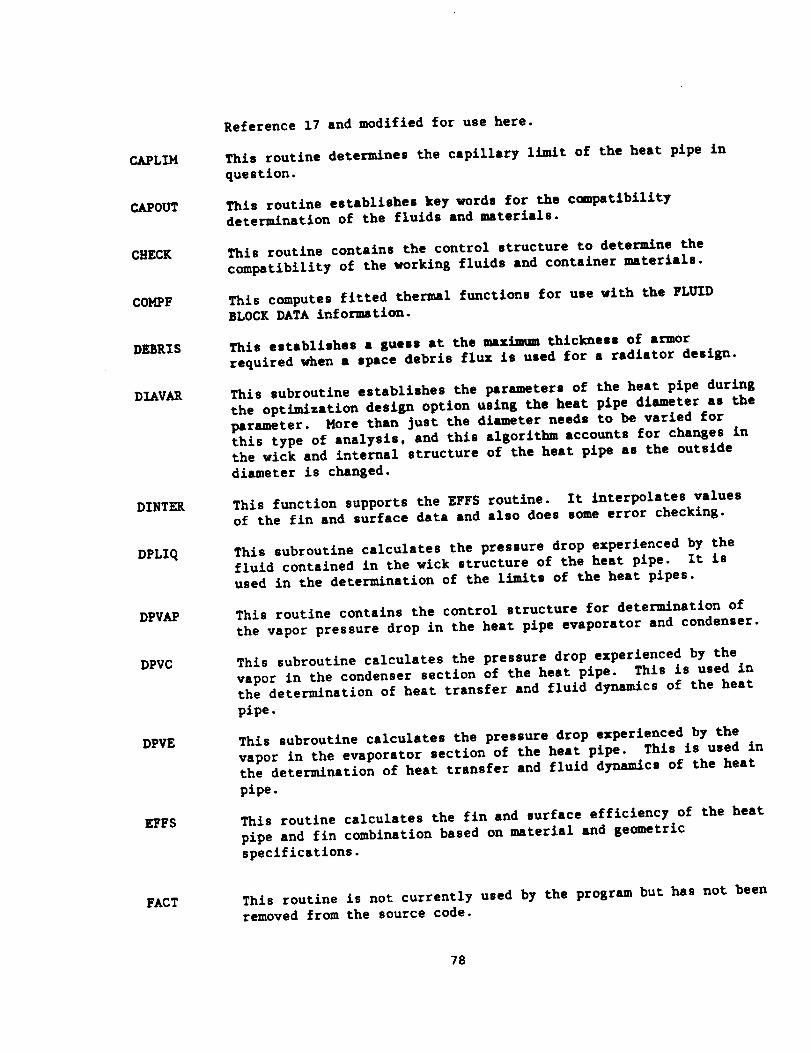
CAPLD4
CAPOUT
CHECK
COHPF
DEBRIS
DIAVAR
DINTER
DPLIQ
DPVAP
DPVC
DPVE
EFFS
Reference 17 and modified for use here.
This routine determines the capillary l_mLtt of the heat pipe in
question.
This routine establishes key words for the compatibilitydetermination of the fluids and materials.
This routine contains the control structure to determine the
compatibility of the workin& fluids and container materials.
This computes fitted thermal functions for use with the FLUIDBLOCK DATA information.
This establishes a suess at the maximum thickness of armor
required when a space debris flux is used for a radiator design.
This subroutine establishes the parameters of the heat pipe durinE
the opt4m4zation design option usin E the heat pipe diameter as theparameter. More than Just the diameter needs to be varied for
this type of analysis, and this algorithm accounts for changes in
the wick and internal structure of the heat pipe as the outside
diameter is chansed.
This function supports the EFFS routine. It interpolates values
of the fin and surface data and also does some error checking.
This subroutine calculates the pressure drop experienced by the
fluid contained in the wick structure of the heat pipe. It is
used in the deterntination of the 14m4ts of the heat pipes.
This routine contains the control structure for determination of
the vapor pressure drop in the heat pipe evaporator and condenser.
This subroutine calculates the pressure drop experienced by the
vapor in the condenser section of the heat pipe. This is used in
the determination of heat transfer and fluid dynamics of the heat
pipe.
This subroutine calculates the pressure drop experienced by the
vapor in the evaporator section of the heat pipe. This is used inthe determination of heat transfer and fluid dynamics of the heat
pipe.
This routine calculates the fin and surface efficiency of the heat
pipe and fin combination based on material and geometricspecifications.
FACT This routine is not currently used by the program but has not beenremoved from the source code.
78

FINDT
FLUX
FRIC
FUNC
GROOVE
HEADER
HEAT
HP
HP1
HPM
HTC
This routine determines the saturation temperature of the fluid
and vapor based on its pressure within the heat pipe. It is used
in the determination of the heat transfer characteristics of the
system.
This subroutine establishes the actual flux (mlcro-meteoroid and
space debris) present for the armor determination.
This subroutine calculates the friction factor required for the
determination of the pressure drop of the fluid in the transportduct.
This subroutine contains the control structure for calculating the
radiator characteristics during the mass minimization option ofthe design algorithm. Allowable temperature drops in a radiator
section are established, and record keeping is done concerning the
heat transfer characteristics of the design.
This subroutine determines the hydrodynamic and thermal propertiesof the groove wick that will be used in the heat transfercalculations.
This subroutine calculates the heat transfer that occurs from the
transport duct of the radiator. The header length is considered
to be only that length of the transport duct that has heat pipeson or in it.
This routine contains the control structure for determination of
the heat transfer of the system. Calculations are done to
determine the required number of heat pipes in a system as well as
temperatures for changing to different heat pipe fluids during the
analysis.
This subroutine calculates the heat transfer capabilities of theheat pipe from the transport duct to the outside of the heat pipe.
This is compared to the heat transfer determined from QSHP, and
temperatures are modified as needed to balance these values.
This routine establishes the choices of possible heat pipe fluids
for a given temperature. This routine is used multiple times An
the interactive input option when the design requires more than
one the heat pipe working fluid to cover the range of temperaturesof the system.
Information concerning the physical details of each heat pipe are
obtained in HPM during interactive input. This also has controlstructure to call other subroutines to obtain all the data to
characterize the heat pipes.
This subroutine determines the convective heat transfer
coefficient of the fluid within the transport duct.
79
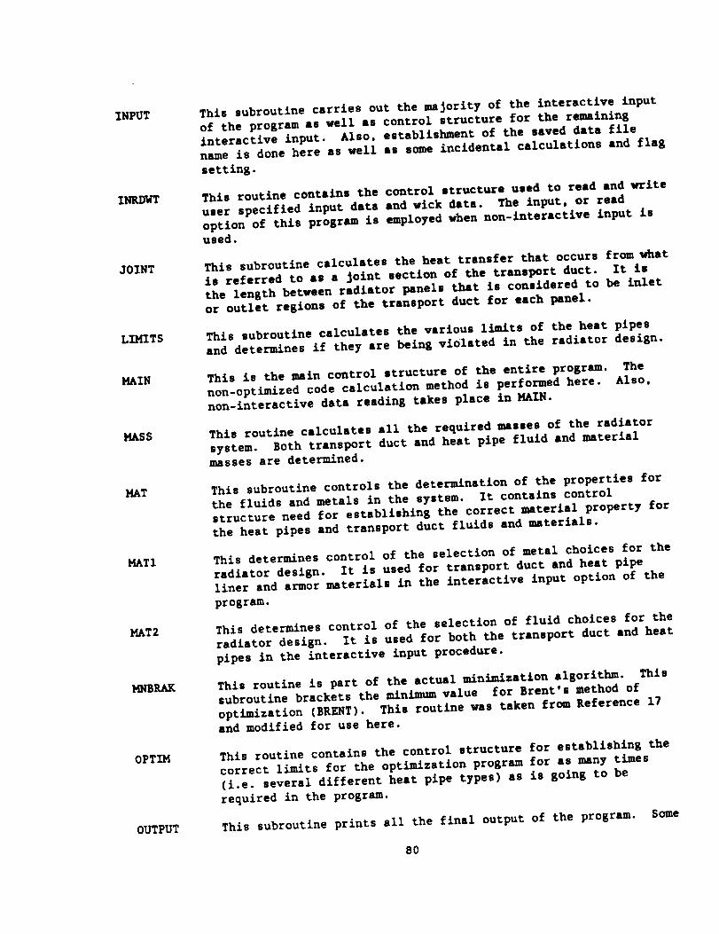
INPUT This subroutine carries out the majority of the interactive input
of the program as well as control structure for the remaining
interactive input. Also, establishment of the saved data file
name is done here as well as some incidental calculations and flag
setting.
INRDWT This routine contains the control structure used to read and write
user specified input data and wick data. The input, or readoption of this program is employed when non-interactive input i8used.
JOINT This subroutine calculates the heat transfer that occurs from what
is referred to as a Joint section of the transport duct. It Is
the length between radiator panels that is considered to be inlet
or outlet regions of the transport duct for each panel.
LL_ITTS This subroutine calculates the various limits of the heat pipesand determines if they are being violated in the radiator design.
MAIN This is the min control structure of the entire program. The
non-optimized code calculation method is performed here. Also,
non-interactive data reading takes place in MAIN.
MASS This routine calculates all the required masses of the radiator
system. Both transport duct and heat pipe fluid and materialmasses are determined.
MAT This subroutine controls the determination of the properties for
the fluids and metals in the system. It contains control
structure need for establishing the correct material property for
the heat pipes and transport duct fluids and materials.
MAT1 This determines control of the selection of metal choices for the
radiator design. It is used for transport duct and heat pipe
liner and armor materials in the interactive input option of the
program.
MAT2 This determines control of the selection of fluid choices for the
radiator design. It is used for both the transport duct and heat
pipes in the interactive input procedure.
MNBRAK This routine is part of the actual minimization algorithm. Thissubroutine brackets the minimum value for Brent'8 method of
optimization (BRENT). This routine was taken from Reference 17and modified for use here.
OPTIM This routine contains the control structure for establishing the
correct limits for the optimization program for as many times
(i.e. several different heat pipe types) as is going to be
required in the program.
OUTPUT This subroutine prints all the final output of the program. Some
8O

calculations, such as pressure drop and specific mass and power
values, are done within this routine to provide the final
specifications of the radiator design.
PROPTH This subroutine determines thermodynamic properties of the heat
pipe fluid vapor stage for use in determ/nlng the heat transfer
resistance in that section of the heat pipe.
QSHP This function determines the heat transfer from the outside of a
heat pipe with a fin attached to it based on assumed temperatures
and emissivities. This heat transfer is compared to the heat
transfer calculated in HP to equate the heat transfer.
SCREEN This subroutine determines the hydrodynamic and thermal properties
of the screen wick (with and without arteries) that will be used
in the heat transfer calculations.
SINTER This subroutine determines the hydrodynamic and thermal properties
of the sintered metal wick (with and without arteries) that will
be used in the heat transfer calculations.
SOLVE This routine is used by ARMOR. It actually calculates the armor
thickness of materials depending on various flags, geometrical
parameters, survival requirements, and redundancies. An IMSL
routine is used in order to calculate the value of a Poisson
distribution in the routine.
SOMETH Determines thermal resistance of the actual heat pipe vapor.
SUBSTR This routine calculates the hoop stress that is present in the
heat pipes and transport ducts.
THERTB2 This routine determines the condensate state point for the heat
pipe fluid.
USER This subroutine is used during the interactive input option to
prompt the code user for material properties when the choice is
made to specify a material that is not available in the built-ln
materials library.
VAPRES
WICK
This subroutine determines the resistance to heat transfer
generated by the vapor when it evaporates and condenses.
This routine obtains the physical and hydraulic characteristics of
the heat pipe wicks during the interactive input.
WIKTHR This subroutine contains the control structure for determination
of the thermal and hydrodynamic characteristics of the heat pipewick structure.
WIKNAT This routine determines the mass of the wick in the heat pipe as
well as other information needed to determine the heat pipe mass.
81

WKEDWTThis routine actually reads and writes the wick data. The read
option of this subroutine is employed when non-interactive input
is used.
82

cEs
. Howell, H.R., et al, "qualification of the Space Shuttle Orbiter
Radiator System", Society of Automotive Engineers Paper No. 820886
(July,1982)
. Stipandic, E.A., 'Spacecraft Application of Heat Pipes', American
Institute of Aeronautics and Astronautics Paper No. 76-241 (April,
1976)
t Presler, A.F., et al, "Liquid Droplet Radiator Program at the NASA Lewis
Research Center", National Aeronautics and Space Administration Report
No. TM 87139 (June, 1986)
t White, K.A., 'Moving Belt Radiator Technology Issues', Proceedings of
the 23rd Intersociety Energy Conversion Engineering Conference, Paper
No. 889132, (July, 1988)
a Carelli, M.D., et al, "The Curie Point Radiator', Proceedings from the
Fifth Symposium on Space Nuclear Power Systems (January, 1988)
. Fraas, A. P., "Protection of Spacecraft from Meteoroids and Orbital
Debris", Oak Ridge National Laboratory Report No. TM-9%04 (March, 1986)
, Lundberg, L. B., et al., "Hypervelocity Impact Studies on
Titanium, Titanium Alloys, and Beryllium', Los Alamos National
Laboratory Report No. LA-9417-MS (August, 1982)
o Frost, V.C., "Meteoroid Damage Assessment', National Aeronautics and
Space Administration Report No. NASA SP-8042 (May, 1970)
o Baker, K.W., Tower, L.K., "The NASA Lewis Heat Pipe Code with
Application to SP-100 GES Heat Pipes', Proceedings from the Fifth
Symposium on Space Nuclear Power Systems (January, 1988)
10. Heat Pi_es, Third Edition, Dunn, P.D., Reay, D.A. Pergamon Press, 1982.
11. Heat P ire Des_._Handbook, B & K Engineering, 1981.
12. Fundamentals of Heat Transfer, Incropera, F. , DeWitt, J., Wiley
Publishing Co., 1981.
13. Eckart, R., Kays, R., 'Radiation Interaction Between a Cylindrically
Finned Surface", ASME Proceedings, 1949.
14. M.J. Schor, "Micro-meteoroids and Space Debris Protection', General
Electric Program Information Release No. U-1810-P2-448, April 1988.
15. N. Elfer, G. Kovacevic, "Design for Space Debris Protection", 3rd AnnualAmerican Institute of Aeronautics and Astronautics Greater New Orleans
Symposium, November, 1985.
85

16.
17.
Handbook o__fHeat Transfer Fundamentals, Third Edition, Rosenhow, M.
editor, McGraw Hill Publishing Co., 1986.
Numerical _ = The b/_ Of _ C_u_.__, Press, W.H., et.
al., Cambrids e University Press, 1986.
84

Nmmd mind
I. me_ctso.NASA CR - 187O67
I I
Report Documentation Page
4. Tib mid_mee,
User's M_u_ for the Heat Pipe Space Pmdiator
Design and Analysis Code (HEPSPAgC)
7. _,)
Donald C. Hainley
L p.,t=,,_ o,w,tmem s._ md_k_mSverdrup Technology, Iuc.
2001 _ Parkway
ikook Park, Ohio 44142
lz a_,mm_ _ .m_ _e _National Aeronautics and Space AdministrationLewis Research Center
Cleveland, Ohio 44135- 3191
+s. _e3tm
s. pwtm,_ oqpn_M_, oee.
None (P.-._74)i i
10. Wink Uldl I_.
505-86-O1-21
i
ll.OWdHlel W Qmmt No.
NAS3 -2.52_
i
I& TYl_ M !_1'1 rand II_iod' Oov_lKI
_Reportlrmal
_4.ag_nm_ A_nw oem
Project Manager, James Calogefas, Power Technology Division, NASA Lewis Research Center, (216) 433-5278. A
floppy diskette with a copy of the Fortran source codes or the Execu_ble Image of HEPSPARC can be obtained bycontacting Karl W. Baker, NASA Lewis Research Ceater, 21000 Brookpark Road, Cleveland, Ohio 44 135,(2 16) 433-5278.
u i
+6. Abmmct
A new computer code has been written for the NASA Lewis Research Cemef named HEPSPARC (which stands for]_,,,at _il_e SPAce Radiator F_de). This code is used fcf the design and amlysis of t rediatcg that is ccam-uct_ from
s pumped fluid loop that transfers heat to the evaporative _ of beat pipes. 'l'uis manual is designed to familiarizethe user with this new code and to serve as a refermge for its use. This numual documents the work ¢kme thus far. It is
also intended to be the first step towards vefifi_tion of the H]F..PSPARC code. Details tre furnished to provide adescription of all the requirements 8nd variables used in the design and analysis of • combined lmmped iooWheat pipe
radiator system. A description of the sulxtmtixms teed in the Wogram is _ for those imerested in tmdemand-ing its detailed workings.
i i
+7. K,,/won_ (sum.rambykmx(s)) lie.
1Spacecraft radiatorsRadiators
Heat pipes
_ mmmmnt
Unchmmed - Unlimited
SubjectCategory 18
*Urea I'ogm tqm OCT am *For rode by the Nation,M Technk:ml Infommtion Se_ioo, Spdngfield, Virginia 22181