7klvhohfwurqlfwkhvlvru … meaning and intrinsic relationship between these ray coordinates and axis...
TRANSCRIPT
This electronic thesis or dissertation has been
downloaded from the King’s Research Portal at
https://kclpure.kcl.ac.uk/portal/
The copyright of this thesis rests with the author and no quotation from it or information derived from it
may be published without proper acknowledgement.
Take down policy
If you believe that this document breaches copyright please contact [email protected] providing
details, and we will remove access to the work immediately and investigate your claim.
END USER LICENCE AGREEMENT
This work is licensed under a Creative Commons Attribution-NonCommercial-NoDerivatives 4.0
International licence. https://creativecommons.org/licenses/by-nc-nd/4.0/
You are free to:
Share: to copy, distribute and transmit the work Under the following conditions:
Attribution: You must attribute the work in the manner specified by the author (but not in any way that suggests that they endorse you or your use of the work).
Non Commercial: You may not use this work for commercial purposes.
No Derivative Works - You may not alter, transform, or build upon this work.
Any of these conditions can be waived if you receive permission from the author. Your fair dealings and
other rights are in no way affected by the above.
Intrinsic Geometry in Screw Algebra and Derivative Jacobian and Their Uses in theMetamorphic Hand
Sun, Jie
Awarding institution:King's College London
Download date: 26. May. 2018

Intrinsic Geometry in Screw Algebra
and Derivative Jacobian and Their
Uses in the Metamorphic Hand
Jie Sun
A thesis submitted in fulfillment of the requirements
for the degree of Doctor of Philosophy
King’s College London, University of London

iii
Abstract
Line geometry is a foundation of screw algebra in line coordinates that were created by
Plücker as ray coordinates taking a line as a ray between two points and axis
coordinates taking a line as the intersection of two planes. This Thesis reveals the
geometrical meaning and intrinsic relationship between these ray coordinates and axis
coordinates, leading to an in-depth understanding of conformability and duality of these
two sets of screw coordinates, and their related vector space and dual vector space.
Based on the study of screw algebra, the resultant twist of a serial manipulator is
presented geometrically by an assembly of unit joint screws with the corresponding
velocity amplitudes. This leads to the geometrical interpretation for the resultant twist
with its instantaneous screw axis (ISA) that is formulated by a combination of weighted
position vectors of joint screws. The screw-based Jacobian is then derived after
recognizing the resultant twist of a serial manipulator. The case leads to a revelation for
the first time the relationship of a Jacobian matrix acquired by using screw algebra and
a derivative Jacobian matrix using differential functions, and to an in-depth
investigation of transformation between these two Jacobians.
To extend the application of screw algebra and this derivative Jacobian, kinematics
analysis of a novel reconfigurable base-integrated parallel mechanism is proposed and
its screw-based Jacobian is derived, leading to its equivalent model, the Metamorphic
hand with a reconfigurable palm. The method is then applied to the investigation of the
iv
Metamorphic Hand, while manipulating an object, based on the product sub-manifolds
and the exponential method. Evaluation of the functionality of the Metamorphic hand
is further analysed, with the Anthropomorphism Index (AI) and palmar shape
modulation as the criteria, evaluating performance enhancement of the Metamorphic
hand in comparison to other robotic hands with a fixed palm.
The Thesis presents novel discoveries in the intrinsic geometry of screw coordinates
and the coherent connection between Jacobian formed by screw algebra and the
Jacobian using the derivative method. This intrinsic geometry insight is then used to
investigate for the first time the parallel mechanism with a reconfigurable base, paving
a way for an in-depth investigation of the Metamorphic hand on its reconfigurability
and grasp affordability and for the first time using Anthropomorphic Index to evaluate
the Metamorphic hand. The Thesis presents a foundation in the study of the
Metamorphic hand.
v
Acknowledgement
I would like to express my sincere gratitude to Prof. Jian S. Dai for his continuous
supports and instructions being a supervisor, and I feel lucky and flattered to be a PhD
student supervised by such an elegant and knowledgeable mentor.
Prof. Dai is a world-class scientist with over 30 years lasting impact in the fields of
mechanisms and robotics. Prof. Dai always tries to solve problems in robotics with
appropriate mathematical methods, in such an elegant way to link robotics with
mathematics, and further with art. This is a philosophy I learn from him beyond my
PhD study. In every talk and meeting with Prof. Dai, I can feel his strong passion and
firm belief to overcome any difficulties on the road of scientific research, which
encourage me all the time during my PhD study and, for sure, every minute in the rest
of my life.
There were so many unforgettable moments over the last few years with Prof. Dai. I
couldn’t forget the first time I met him in ROBIO 2011 in Tianjin, China, when I was
an undergraduate and I felt horned and nervous to get the acquaintance of such a famous
scholar. And then one month later, we met again in Washington D.C., USA, when I
attended the student robotics competition in ASME 2011 IDETC. I won the first place
award and received his warm congratulations. At that time, I made up my mind to
pursue my PhD under his supervision. The next stories were Prof. Dai gave me great
supports for applying for a scholarship at King’s, guided me carrying out research,
offered me so many opportunities to attend summer schools and conferences, assisted
vi
me in writing and revising papers, etc. I would like to thank Prof. Dai again for all these
good memories and his great help and guidance not only in research but also every
aspect of my life.
I also want to thank Dr. Guowu Wei and Dr. Ketao Zhang. I had great experiences
working with Guowu and Ketao in TOMSY project and SQUIRREL project. As former
research assistants, they gave unlimited help to new students like me, created a
favorable atmosphere in my group, and provided detailed orientation. I enjoyed every
moment discussing and working with them. Now Guowu is a lecturer in Salford
Universiy and Ketao leaves for Imperial College for another research position. Though
I cannot meet them very often, memories always stay.
I must thank Mr. Xinsheng Zhang, who are not only a colleague in my group but also
the closest friend to me in London. Xinsheng has a solid theoretical background and
deep understanding in screw theory, lie group and lie algebra. We always study and
discuss together, and recently when the SQUIRREL project brings him in, we work
together as well. I appreciate very much for having such a loyal friend and the friendship
he gives me.
I also want to give my thanks to Dr. Chen Qiu, Dr. Evangelos Emmanouil, and Dr.
Vahid Aminzadeh, with whom I work in my PhD study. Chen has keen senses of smell
on research and always works hard. He generates very good results during his PhD and
is a model I need to learn from. Vahid guided me to the lab when I entered the group
and answered all my questions regarding equipment and resources in the lab. I took
vii
over Evangelos’s work in SQUIRREL project when he graduated, and he gave me
instructions patiently.
Apart from my supervisor and colleagues, I would like to thank other researchers in the
Centre for Robotics Research, particularly Dr. Peng Qi, Dr. Shan Luo, Mr. Xiaozhan
Yang, and faculty members in Department of Informatics, particularly Dr. Hongbin Liu,
Dr. Matthew Howard, Dr. Helge Wurdemann who is a lecturer in University College
of London, and Prof. Kaspar Althoefer who moves to Queen Mary University of
London recently. Also thank my friends Mr. Liqiang Fan, Mr. Dabo Chen, Ms. Yile
Wu, and Ms. Zhen He for all the friendships and love.
I must give my sincere thanks to King’s College London who accepts me as a PhD
candidate and provides me the full scholarship, King’s China Award, to cover my
tuition fee and living costs for three years of my PhD study.
I also want to acknowledge the support during writing-up from the European
Commission 7th Framework Project SQUIRREL “Clearing Clutter Bit by Bit” under
Grant No. 610532.
At last, special thanks must be given to my parents Mr. Jiuwen Sun and Mrs. Yuhua
Liu, who always support and encourage me at my back unconditionally, and the love
from family is always the greatest motivation for me to move forward.

viii
Table of Contents
Abstract ....................................................................................................................... iii
Acknowledgement ........................................................................................................ v
Table of Contents ...................................................................................................... viii
List of Figures ........................................................................................................... xiii
List of Tables .............................................................................................................. xv
List of Symbols .......................................................................................................... xvi
Chapter 1 Introduction ........................................................................................... 1
1.1 State of the Problem ........................................................................................ 1
1.2 Aims and Objectives ....................................................................................... 3
1.3 Organization of the Thesis .............................................................................. 4
Chapter 2 Background ............................................................................................ 8
2.1 Introduction ..................................................................................................... 8
2.2 Line Geometry and Screw Coordinates .......................................................... 8
2.3 Methodologies on First-Order Kinematics Analysis .................................... 10
2.4 Reconfigurable Base-Integrated Parallel Robots .......................................... 12
2.5 Metamorphic Hand with a Reconfigurable Palm ......................................... 14
2.5.1 The Dexterous Hands ............................................................................ 15
2.5.2 Dexterous Hands with a Reconfigurable Palm ...................................... 17
2.5.3 The Metamorphic Hands ....................................................................... 18
2.5.4 Grasping Affordance ............................................................................. 19
2.6 Conclusions ................................................................................................... 20
Chapter 3 Geometry of Screw Coordinates ........................................................ 22
3.1 Introduction ................................................................................................... 22
3.2 Position Vectors and Their Triangular Resultant for Ray Coordinates ........ 23
3.3 Projected Triangle for Axis Coordinates with Weighted Plane Normals ..... 27
3.3.1 Duality in Point-Plane Representations of a Line ................................. 27
3.3.2 Algebraic Derivation of Axis Coordinates ............................................ 30
3.3.3 Geometrical Presentation of Axis Coordinates ..................................... 32
3.4 Conclusions ................................................................................................... 34
Chapter 4 Geometrically Intrinsic Connections of Screw Coordinates ........... 36
ix
4.1 Introduction ................................................................................................... 36
4.2 Form and Geometry Conformability of Two Sets of Coordinates ............... 36
4.3 Correlated Ratio Relationships ..................................................................... 39
4.4 Correlation Coefficient and Correlation Operator ........................................ 42
4.5 Duality and Conformability .......................................................................... 45
4.6 Conclusions ................................................................................................... 47
Chapter 5 Geometrical Meaning of a Twist Based on Screw Algebra ............. 49
5.1 Introduction ................................................................................................... 49
5.2 Homogenous Coordinates of Screws as 6-Dimensional Vector ................... 50
5.2.1 Homogenous Screw Coordinates .......................................................... 50
5.2.2 Screw System of nth Order ..................................................................... 52
5.3 The Helicoidal Velocity Field ....................................................................... 52
5.4 Linear Velocity from a Twist ........................................................................ 54
5.4.1 Point on a Rigid Body Coincident with the Reference Point ................ 54
5.4.2 Geometrical Meaning of Secondary Part of a Screw ............................ 56
5.4.3 Position Vector of the Resultant Twist .................................................. 59
5.4.4 Coordinated ISA of the End-Effector of a Serial Manipulator .............. 60
5.5 Screw based Jacobian Derivation of Serial Robots ...................................... 62
5.5.1 Jacobian Matrix of a Planar Serial Manipulator .................................... 62
5.5.2 Resultant Twist of a Spatial Serial Manipulator .................................... 64
5.6 Conclusions ................................................................................................... 65
Chapter 6 Geometrical Interpretation of the Transformation between Robot Jacobian and Screw Jacobian ................................................................................... 66
6.1 Introduction ................................................................................................... 66
6.2 Derivative Method based Jacobian of a 3R Planar Serial Manipulator ........ 67
6.2.1 Linear Velocity of a 3R Planar Serial Manipulator ............................... 67
6.2.2 Jacobian Generation based on the Derivative Method .......................... 68
6.3 Reconciliation of the Jacobian based on Screw Algebra and Derivative Method .................................................................................................................... 69
6.3.1 Transformation Using a Skew-Symmetric Matrix ................................ 69
6.3.2 Reconciliation of the Jacobian of a 3R Serial Manipulator ................... 71
6.4 Reconciliation of Jacobian Matrices a Spatial Serial Manipulator ............... 73
6.4.1 Screw Algebra based Jacobian for a Spatial Serial Manipulator........... 73
6.4.2 Transformation Matrices of a Spatial Serial Manipulator ..................... 76
6.4.3 Derivative Method based Jacobian for a Spatial Serial Manipulator .... 78
x
6.5 Conclusions ................................................................................................... 80
Chapter 7 Screw Jacobian Analysis of a Reconfigurable Platform-Based Parallel Mechanism ................................................................................................... 81
7.1 Introduction ................................................................................................... 81
7.2 A Spherical-Base Integrated Parallel Mechanism ........................................ 82
7.2.1 From Manipulation with a Metamorphic Hand to a Parallel Mechanism with a Reconfigurable Base ............................................................................... 82
7.2.2 Structure of the Spherical-Base Integrated Parallel Mechanism ........... 83
7.3 Mechanism Decomposition and Geometric Constraints of the Spherical-Base Integrated Parallel Mechanism ............................................................................... 84
7.3.1 Constraint Equations of the Reconfigurable Base ................................. 85
7.3.2 Position of the 3-RRS Parallel Mechanism in a Particular Configuration of the Reconfigurable Base ................................................................................ 90
7.3.3 Forward Kinematics of the Spherical-base Integrated Parallel Mechanism ......................................................................................................... 91
7.4 Inverse Kinematics of the Spherical-Base Integrated Parallel Mechanism .. 95
7.5 Screw Theory based Jacobian Analysis ...................................................... 100
7.5.1 Jacobian Analysis for the Reconfigurable Base .................................. 100
7.5.2 Screw-based Jacobian Analysis for the Spherical-Base Integrated Parallel Mechanism .......................................................................................... 101
7.5.3 Velocity of the Spherical-Base Integrated Parallel Mechanism .......... 104
7.6 Conclusions ................................................................................................. 107
Chapter 8 Screw Embedded Jacobian and Exponential Mapping of Grasp Affordability with a Reconfigurable Palm ............................................................ 109
8.1 Introduction ................................................................................................. 109
8.2 Structure of a Mobile Manipulator with a Metamorphic Robotic Hand ..... 110
8.3 Kinematics of the Metamorphic Hand and the Serial Manipulator ............ 112
8.3.1 Geometry and Kinematics of the Articulated Reconfigurable Palm ... 113
8.3.2 Kinematics of the 7-DOF Serial Robot ............................................... 115
8.3.3 Palm Integrated Kinematics of the Metamorphic Hand and the Manipulator ...................................................................................................... 119
8.4 Metamorphic Hand based Grasp Constraints ............................................. 121
8.4.1 Form of Grasp Map and Grasp Constraints ......................................... 122
8.4.2 Grasp Constraints of the Metamorphic Hand ...................................... 123
8.5 Grasp Affordance Related to the Manipulator Kinematics and Grasp Constraints ............................................................................................................ 127
8.5.1 Grasp Affordance based on Object Models ......................................... 127
xi
8.5.2 Relation of Grasp Affordance to the Manipulator Kinematics and Grasp Constraints ....................................................................................................... 129
8.6 Conclusions ................................................................................................. 131
Chapter 9 Geometric Topology with Product Submanifolds on Metamorphic Hand Grasping ......................................................................................................... 132
9.1 Introduction ................................................................................................. 132
9.2 Product Submanifolds and its Tangent Space ............................................. 133
9.2.1 Product Submanifolds of SE(3) ........................................................... 133
9.2.2 Tangent Spaces of Product Submanifolds ........................................... 135
9.2.3 10 Lie Subgroups of SE(3) .................................................................. 137
9.3 Operation of Lie Group for Metamorphic Hand Grasping ......................... 138
9.3.1 Topology Diagram for the Metamorphic Hand ................................... 138
9.3.2 Lie Group Operations on Hand-Object Model .................................... 139
9.4 Conclusions ................................................................................................. 143
Chapter 10 Geometry Variation Entailed Metamorphic Hand Benchmarking and Anthropomorphism Index ............................................................................... 144
10.1 Introduction ................................................................................................. 144
10.2 Kinematic Transverse Arch of the Metamorphic Palm .............................. 145
10.2.1 The Kinematic Transverse Arch of Human Hands ............................. 145
10.2.2 Transverse Arch Inspired Palm Geometry Variation Analysis ........... 147
10.2.3 The Palm Geometry Variation related Actuation Constraints ............. 148
10.2.4 Geometric Constraints of the Metamorphic Palm ............................... 150
10.3 Arch Measurement of the Metamorphic Palm ............................................ 152
10.4 Palm Geometry Variation based Workspace of the Metamorphic Hand .... 155
10.5 Hand Model Generation and Simplification for Benchmarking ................. 160
10.5.1 Hand Model Generation ...................................................................... 160
10.5.2 Hand Model Simplification ................................................................. 161
10.6 Measurement Indexes and Criteria ............................................................. 162
10.6.1 Projection based Measurement Indexes .............................................. 162
10.6.2 Evaluation of the Metamorphic Hand based on AI ............................. 163
10.6.3 The Improvement of AI with the Reconfigurable Palm ...................... 163
10.7 Comparison of the Metamorphic Hand with Selected Robotic hands ........ 165
10.7.1 The Effect of Number of DODs .......................................................... 165
10.7.2 The Effect of Distribution of DOFs ..................................................... 166
10.7.3 The Influence of Sampling Density on AI .......................................... 167
10.7.4 AI Analysis According to Different Palm Configurations .................. 168

xii
10.8 Conclusions ................................................................................................. 169
Chapter 11 Conclusions ..................................................................................... 171
11.1 General Conclusions ................................................................................... 171
11.2 Contributions and Main Achievements of the Thesis ................................. 174
11.3 Future Works .............................................................................................. 177
List of Publications .................................................................................................. 179
References ................................................................................................................ 181
Appendix A ............................................................................................................... 195
Appendix B ............................................................................................................... 196
Appendix C ............................................................................................................... 198
xiii
List of Figures
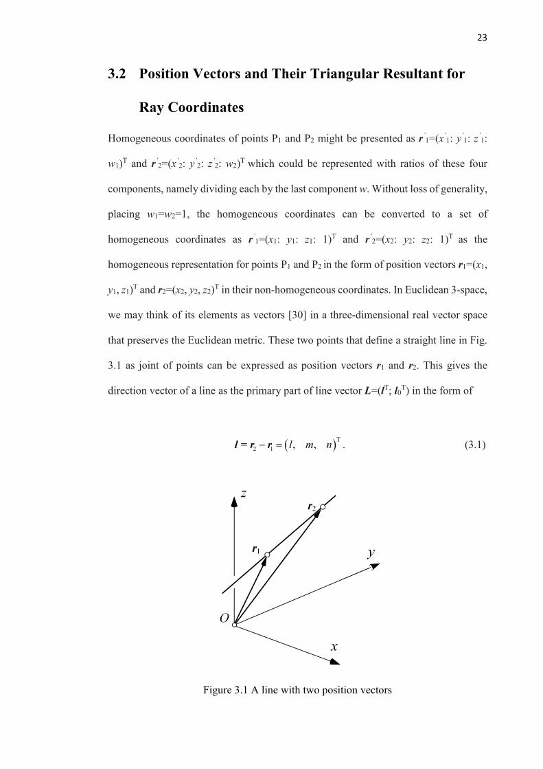
Figure 3.1 A line with two position vectors ................................................................ 23
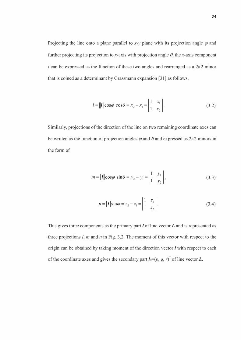
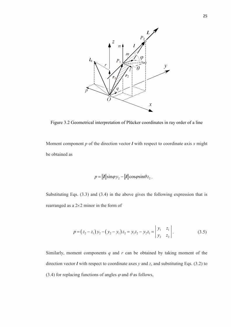
Figure 3.2 Geometrical interpretation of Plücker coordinates in ray order of a line ... 25
Figure 3.3 A line as the intersection of two planes ..................................................... 28
Figure 3.4 Geometrical interpretation of the axis coordinates .................................... 33
Figure 4.1 Integrated geometrical presentations of ray and axis coordinates ............. 37
Figure 4.2 Conformability graph ................................................................................. 45
Figure 5.1 Instantaneous screw axis and the helicoidal velocity field ........................ 53
Figure 5.2 A Twist modeled by a revolute joint of a rigid body ................................. 55
Figure 5.3 Geometry representation of a resultant twist in a serial manipulator......... 56
Figure 5.4 A 3R planar serial manipulator .................................................................. 63
Figure 6.1 Screw coordinates with respect to the global reference frame of A RRPRR
spatial serial manipulator ............................................................................................. 74
Figure 6.2 A spatial 5-DOF RRPRR serial manipulator ............................................. 76
Figure 7.1 Object manipulated by a three-fingered metamorphic hand ...................... 83
Figure 7.2 Structure of the spherical-base integrated parallel mechanism .................. 84
Figure 7.3 The reconfigurable base of the spherical-base integrated parallel
mechanism ................................................................................................................... 86
Figure 7.4 Kinematic analysis for limb 2 of the spherical-base integrated parallel
mechanism ................................................................................................................... 94
Figure 7.5 Motion screw of the spherical-base integrated parallel mechanism ........ 102
Figure 7.6 Motion screw of closed-loop mechanism decomposed from the parallel
mechanism ................................................................................................................. 105
Figure 8.1 Structure of a mobile manipulator with a metamorphic robotic hand ..... 111
Figure 8.2 The articulated reconfigurable palm and its geometry ............................. 113
Figure 8.3 Geometry of the mobile manipulator in the reference position. .............. 116
Figure 8.4 Grasp a disk with the three-fingered Metamorphic hand ......................... 119
Figure 8.5 Relations of grasp affordance, manipulator kinematics and grasp constraint
................................................................................................................................... 130
xiv
Figure 9.1 The relationship among the complex, submanifold, and subgroup of SE(3)
................................................................................................................................... 134
Figure 9.2 A commutative diagram for the product submanifold, the submanifolds,
and the related tangent spaces ................................................................................... 136
Figure 9.3 Lie group built-in topology diagram for the hand-object system with a
reconfigurable base .................................................................................................... 139
Figure 9.4 A simplified topology diagram by merging the subgroups of finger 2 and 3
................................................................................................................................... 141
Figure 9.5 A simplified topology diagram by merging all the subgroups of finger 1, 2
and 3 .......................................................................................................................... 142
Figure 9.6 The final deducted topology diagram of the Metamorphic hand with
grasped object ............................................................................................................ 143
Figure 10.1 Arches of human hand, (a) Human palm arches, (b) The kinematic
transverse arches ........................................................................................................ 146
Figure 10.2 The kinematic transverse arch of the metamorphic palm ...................... 147
Figure 10.3 The Metamorphic hand with a reconfigurable palm .............................. 149
Figure 10.4 The range of θ1 with respect to the changes of θ5 .................................. 152
Figure 10.5 The contributions of the thenar arch, hypothenar arch in kinematic
transverse arches at the change of θ1 when θ5 = 120° ............................................... 153
Figure 10.6 The kinematic transverse arch of the reconfigurable palm .................... 154
Figure 10.7 The workspace of the thumb and other fingers processed with Delaunay
triangulation method. (a) The workspace of index finger, middle finger, ring finger
and little finger. (b) The workspace of the thumb ..................................................... 156
Figure 10.8 The workspace of the whole hand with two palm actuation angles as
θ5=π/2, θ1=-2π/3 ........................................................................................................ 157
Figure 10.9 The functional workspace of each finger ............................................... 158
Figure 10.10 The functional workspace with different θ1 when θ0 = π/2, 2π/3 and 5π/6
................................................................................................................................... 159
Figure 10.11 The model of the Metamorphic hand ................................................... 161
Figure 10.12 Projection of the Metamorphic hand to the latent space. (a) The
projection of the Metamorphic hand with the reconfigurable palm; (b) The projection
of the Metamorphic hand with the freezed reconfigurable palm (θ3 = θ4 = 0) .......... 164
Figure 10.13 The value of AI with fixed sample size and various sampling density 168
Figure 10.14 The value of AI with different palm configurations ............................ 169

xv
List of Tables
Table 4.1 Duality and conformability ......................................................................... 46
Table 8.1 Joint twists of the 7-DOF serial robot ...................................................... 117
Table 9.1 Proper lie subgroups of SE(3) with motion types ...................................... 137
Table 10.1 The AI of four robotic hands evaluated by the toolbox .......................... 166
xvi
List of Symbols
L A line vector
lT The primary part of a line vector
l0T The secondary part of a line vector
D The correlation operator
se(3) Lie algebra of the special Euclidean group of 3-dimensional
Euclidean space
Si Screw associated with the ith joint
Sij Screw associated with the jth joint in the ith limb
si The direction vector of a screw associated with the ith joint
s0 The secondary part of a screw
h The pitch of a screw
ε Dual unit of dual vector
3 3-dimensional affine space
3 3-dimensional projective space
V6 6-dimensional vector space
n Screw system of order n
Ti The twist of associated the ith joint
Js Screw-based Jacobian matrix
JD Derivative method-based Jacobian matrix
Jh Hand Jacobian matrix
iTj Transformation matrix from the ith coordinate frame to the jth
coordinate frame
xvii
R(xi,φi) A 3×3 rotation matrix that represents a rotation about xi-axis by φi
PA Position vector of point A in the global coordinate frame
FCiP The position vector of point Ci (i = 1, 2 and 3) with respect to
global coordinate frame F
aθ The velocity vector of active joints
i The change rate of the ith joint
SE(3) The special Euclidean group of 3-dimensional Euclidean space
SO(3) The special orthogonal group of 3-dimensional Euclidean space
[d×] Skew-symmetric matrix of vector d
Adg Adjoint transformation associated with g
[ ]1 1eS
Exponential map from Lie algebra to Lie group
T (u) Lie subgroups of SE(3)
M Product submanifold of SE(3)
Bci The wrench basis corresponding to different contact types
bpoV
The body velocity of the object expressed in a global reference
frame
Gi Grasp matrix of the ith finger
Tgx A grasp executed by the Metamorphic hand
αi The angle of the ith link in the palm of the Metamorphic hand
MW Workspace of fingers in the Metamorphic hand
FW Functional workspace of the Metamorphic hand
1
Chapter 1 Introduction
1.1 State of the Problem
Line geometry is a foundation for screw theory. Homogenous coordinates can be used
to present a line in space, known as a line vector. Line coordinates are then extended
by Plücker to ray coordinates and axis coordinates, namely a line as a ray between two
points and a line as the intersection of two planes. A screw is formed by adding the
primary part with a scalar known as a pitch to the secondary part of a line vector. As a
geometrical entity, a screw in the form of six coordinates can carry a twist by associating
a velocity amplitude or carry a force by a force intensity, in such ways to obtain the
physical meanings in mechanism and robot analysis.
Though Plücker coordinates in ray order are well received, their counterpart in axis
order is relatively not well known and, in particular, the geometrical meaning of ray
coordinates and axis coordinates are not well revealed. Moreover, the duality and
intrinsic relationship between ray coordinates and axis coordinates still remain unclear.
The explicit relation between the relevant vector space and dual vector space needs to
be investigated for acquiring the geometrical interpretation between the two set of
Plücker.
Based on line geometry, screw theory is developed and plays a key role in mechanics
and mechanisms. As a twist can be regarded as a unit screw associating a velocity
2
amplitude, the kinematics analysis of mechanisms is closely linked to the application
of screw algebra. In particular, the twist of the end-effector of a serial manipulator is
the assembly of unit joint screws with the corresponding joint changing rates. In a
different way, the Denavit-Hartenberg method is also well-known to formulate the
position of the end-effector, as well as the first-order kinematics by taking its time
derivative. The relation of velocities and Jacobian matrices acquired by the derivative
method and screw algebra is not well presented, and the transformation between the
two Jacobian needs to be further investigated.
There have been substantial interests in kinematics analysis of multifingered hands. The
metamorphic hand is developed to achieve higher performance and graspability by
involving a reconfigurable palm. Instead of considering the hand kinematics in
isolation, an equivalent transformation to map the hand-object system to a parallel
mechanism integrated with a reconfigurable base is conducted through treating the non-
sliding contact between a fingertip and the grasped object as a spherical pair. In such a
way, the Metamorphic hand with a grasped object is regarded as a typical parallel
mechanism with a reconfigurable base. Then the methodologies to study parallel
mechanism can be migrated to understanding the motion of the grasped object. Screw
theory is adopted to formulating the base geometry variation of the reconfigurable
parallel mechanism, and the influence of reconfigurable base on the moving platform
also needs to be studied by Jacobian analysis.
The grasping matrix of the metamorphic hand needs to be explored to establish a
mathematics model for the further study of grasping affordance. Product-of-exponential
mapping and topology based product submanifolds are also appropriate tools to build
3
the mathematical model and highlight the enhancement of the integrated flexible palm
in terms of grasping and manipulation.
Furthermore, evaluation of the performance of the Metamorphic hand has to be
considered to demonstrate the improvement of dexterity by involving this
reconfigurable palm. Comparison and reconciliation between the human palm and the
reconfigurable palm are crucial to reveal the intrinsic advancement of this flexible palm.
To assess the palmar shape modulation through transverse metacarpal arch inspired by
human hands, the favorable palm configuration can be found for the best fit of finger
grasping positions. The Anthropomorphism Index is also proposed to compare different
hand constructions in such a way to verify the advantages of a robotic hand with a
flexible palm.
1.2 Aims and Objectives
The thesis emphasizes the intrinsic geometry connection of screw coordinates and the
formulation of Jacobians with different methods, followed by their relation and
transformation. The thesis also applies these mathematical tools to analyzing the grasp
matrix of the Metamorphic hand and evaluating its performance.
The objectives of this thesis are listed as follows,
a) Reveal the interrelation of the line coordinates and give the intrinsic geometrical
interpretation of the correlation operator widely used in screw algebra.
b) Study the duality and conformability of the screw coordinates, as well as the
insight of its representation in vector space and dual vector space.

4
c) Explore the geometrical meaning of a twist and the transformation between the
screw-based Jacobian and derivative method-based Jacobian.
d) Investigate kinematics of the reconfigurable platform based-parallel mechanism
and the Jacobian analysis by means of screw algebra.
e) Develop the grasping matrix and grasping affordance of the Metamorphic hand
with the product-of-exponential method.
f) Present the topological evolution of the Metamorphic hand with grasped object
model with product submanifolds operations.
g) Evaluate the performance of the Metamorphic hand by a nonlinear data
reduction model and a palmar shape modulation migrated from human palm
variation.
1.3 Organization of the Thesis
This thesis is organized into 11 chapters, and brief introduction and construction of each
chapter is presented as follows,
Chapter 1 is the introduction of this thesis where the state of problems, aims and
objectives, and its organization are described.
Chapter 2 covers the background of this thesis, state-of-the-art and the problems going
to be investigated in the following chapters. The background includes a brief
introduction to line geometry and screw coordinates, the mathematical methods to study
the first-order kinematics of a robot, the typical parallel robots, and reconfigurable base-
integrated parallel robots, and the development of dexterous robotic hands and the
Metamorphic hand with a reconfigurable palm.
5
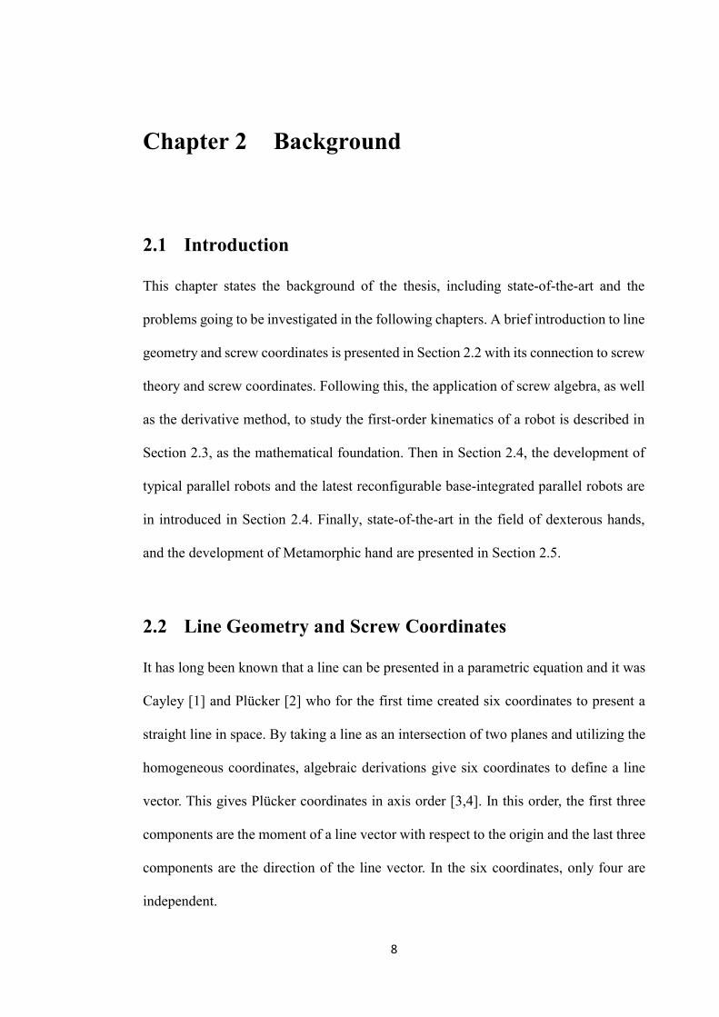
Chapter 3 introduces screw coordinates and their geometrical interpretation. In order
to reveal the geometrical insight in Euclidean 3-space, homogeneous coordinates of a
point and a plane are converting to a set of homogeneous coordinates with the last
component as 1, using ratios of homogeneous coordinates. A line joined by two points,
which produces ray coordinates, and a line intersected by two planes, which produces
axis coordinates, are formulated, and the geometrical meaning of each single
component in these two sets of coordinates is given.
Chapter 4 reveals the intrinsic connection between ray coordinates and axis coordinates.
The interrelation of the two sets of coordinates and their conformability are investigated
through their geometrical representation. Further, the correlated ratio relationships and
a corresponding correlation coefficient of the coordinates are studied, followed by a
correlation operator to link the vector space with dual vector space in where the two
sets of coordinates are formed. The intrinsic relation of the ray coordinates and axis
coordinates are summarized in a duality and conformability table.
Chapter 5 presents the geometrical meaning of a twist and the geometrical
representation of a resultant twist assembled by unit joint screws with their
corresponding velocity amplitudes. The instantaneous screw axis of the resultant twist
is coordinated, and its position vector is obtained. The Jacobian matrix of a planar serial
manipulator is derived followed by the generation of a resultant twist of a spatial serial
manipulator.

6
Chapter 6 derives the transformation between the screw-based Jacobian matrix and the
derivative method-based Jacobian matrix of a serial manipulator. Through the
investigation of the linear velocity of a serial manipulator, reconciliation of the
Jacobians based on screw algebra and derivative method is formulated with their
geometrical interpretation. At last, a spatial serial manipulator is exampled to verify the
proposed transformation method.
Chapter 7 proposes a parallel mechanism with a reconfigurable base for the first time.
The base of this parallel mechanism is formed by a spherical five-bar linkage
mechanism, which provides augmented motion for each limb. Structure design of the
proposed spherical-base integrated parallel mechanism is introduced, and geometry and
kinematics of the mechanism are investigated leading to closed-form solutions of
kinematics. Screw theory-based Jacobian is then presented in the form of partitioned
matrix followed by the velocity analysis.
Chapter 8 presents the construction of the mathematical model of the Metamorphic
hand grasping an object. The kinematics of a 7-DOF serial manipulator is also proposed
with its last link attached the Metamorphic hand. The grasping matrix of the hand is
established with the screw embedded Jacobian and product-of-exponential method. The
preliminary study of grasping affordance of the hand is also presented with its relation
to the manipulator kinematics.
Chapter 9 presents the grasping model of the Metamorphic hand manipulating an object.
Apart from introducing the 10 corresponding Lie subgroups, product submanifolds of
Lie group SE(3) and Lie subgroup built-in topology diagram are defined with operation
7
rules. Based on the topological model of the hand-object system, the operation of Lie
group is implemented to simplify the topology diagram of the Metamorphic hand by
merging the product submanifolds of two adjacent fingers in a recursive way.
Chapter 10 uses a nonlinear dimension reduction model, Gaussian Process Latent
Variable Model (GPLVM), to project the high dimension fingertip data to a 2D latent
plane in such a way to evaluate robotic hands and carry out the comparison among
different hands. A different way relates the Metamorphic palm to the human palm with
transverse metacarpal arch, which acts as a new approach to evaluate a robotic hand
with palmar shape modulations. Then the functional workspace, as an indicator
evaluating the precise manipulation of the metamorphic hand, is extended to show the
impact of palm arch on graspability.
8
Chapter 2 Background
2.1 Introduction
This chapter states the background of the thesis, including state-of-the-art and the
problems going to be investigated in the following chapters. A brief introduction to line
geometry and screw coordinates is presented in Section 2.2 with its connection to screw
theory and screw coordinates. Following this, the application of screw algebra, as well
as the derivative method, to study the first-order kinematics of a robot is described in
Section 2.3, as the mathematical foundation. Then in Section 2.4, the development of
typical parallel robots and the latest reconfigurable base-integrated parallel robots are
in introduced in Section 2.4. Finally, state-of-the-art in the field of dexterous hands,
and the development of Metamorphic hand are presented in Section 2.5.
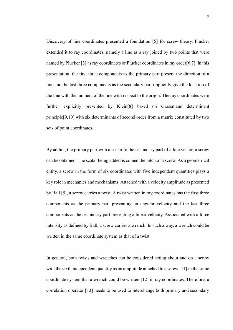
2.2 Line Geometry and Screw Coordinates
It has long been known that a line can be presented in a parametric equation and it was
Cayley [1] and Plücker [2] who for the first time created six coordinates to present a
straight line in space. By taking a line as an intersection of two planes and utilizing the
homogeneous coordinates, algebraic derivations give six coordinates to define a line
vector. This gives Plücker coordinates in axis order [3,4]. In this order, the first three
components are the moment of a line vector with respect to the origin and the last three
components are the direction of the line vector. In the six coordinates, only four are
independent.
9
Discovery of line coordinates presented a foundation [5] for screw theory. Plücker
extended it to ray coordinates, namely a line as a ray joined by two points that were
named by Plücker [3] as ray coordinates or Plücker coordinates in ray order[6,7]. In this
presentation, the first three components as the primary part present the direction of a
line and the last three components as the secondary part implicitly give the location of
the line with the moment of the line with respect to the origin. The ray coordinates were
further explicitly presented by Klein[8] based on Grassmann determinant
principle[9,10] with six determinants of second order from a matrix constituted by two
sets of point coordinates.
By adding the primary part with a scalar to the secondary part of a line vector, a screw
can be obtained. The scalar being added is coined the pitch of a screw. As a geometrical
entity, a screw in the form of six coordinates with five independent quantities plays a
key role in mechanics and mechanisms. Attached with a velocity amplitude as presented
by Ball [5], a screw carries a twist. A twist written in ray coordinates has the first three
components as the primary part presenting an angular velocity and the last three
components as the secondary part presenting a linear velocity. Associated with a force
intensity as defined by Ball, a screw carries a wrench. In such a way, a wrench could be
written in the same coordinate system as that of a twist.
In general, both twists and wrenches can be considered acting about and on a screw
with the sixth independent quantity as an amplitude attached to a screw [11] in the same
coordinate system that a wrench could be written [12] in ray coordinates. Therefore, a
correlation operator [13] needs to be used to interchange both primary and secondary
10
parts of a wrench to form a reciprocal product to complete the work done by a wrench
on a twist. This is essential in working out the reciprocity or work done in robotics[14-
16] and in mechanism analysis and synthesis [18-20].
Expressing a wrench in axis coordinates and a twist in ray coordinates leads to two
spaces. In a modern approach, a twist is defined as an element of the Lie algebra of the
group of rigid-body displacement and a wrench as an element of the dual Lie algebra
that has the primary part presenting a moment and the secondary part presenting a force,
presented in a vector space of all those dual elements, as a dual vector space. In other
literature[21,22], a wrench in axis coordinates is referred to a co-screw in an isomorphic
vector space, as a dual vector space.
Though Plücker coordinates in ray order is well received, its counterpart in axis order
is relatively not well known and in particular, the geometrical meaning of ray
coordinates particularly axis coordinates has not yet been revealed. Further, though
duality of a line on its self-dual [14] was stated, the duality and intrinsic relationship
between ray and axis coordinates have not yet been revealed. Hence, the geometrical
meaning of the relationship particularly line geometry still needs to be revealed and to
give the insight to screw property[23-26] and mechanism development[27-29].
2.3 Methodologies on First-Order Kinematics Analysis
Kinematics analysis is the fundamental topic in robotics and studying the kinematics of
a manipulator is a necessary procedure to understand its functionality and performance.
Forward kinematics establishes the mathematical relation to map the joint
displacements to the position and orientation of the end-effector of a manipulator,
11
whereas the inverse kinematics relates the end-effector configuration to joint
movements. Differentiating the forward kinematics equation gives the Jacobian matrix
that formulates the velocity map between joint rates and the velocity state of the end-
effector. The Jacobian portrays the velocity map from joint space to task space of a
manipulator which can be used to identify the singularly, generate the desired trajectory
with an appropriate speed, etc. There are several ways to construct the Jacobian of a
serial manipulator in the literature[65], the most popular ones are the derivative
methods[103] and the screw theory based method[65].
The conventional way to generate Jacobian of a manipulator with the derivative method
is to formulate the forward kinematics analysis by the transformation matrices or the
geometrical relation first, and then take the time derivative of position and orientation
of the end-effector. The transformation matrices that depict the rotation and translation
of coordinate frames attached in contiguous links can be developed with D-H
parameters[102]. By multiplying transformation matrices in an order, the gesture of the
tool frame fixed on the end-defector is revealed with respect to the global coordinate
frame though joint displacements and the geometry of the manipulator. As the position
and orientation of the end-effector are functions of joint displacements, taking its time
derivative will result in the translational velocity and angular velocity expressed by the
joint rates and the geometry of the manipulator, in which way the conventional Jacobian
is developed.
Screw theory is another way to carry out forward velocity analysis of a serial
manipulator. By investigating the line geometry, Plücker [2] and Cayley [1] used the
homogenous coordinates to represent a straight line in space, of which the first three
12
coordinates indicate the direction of the line and the last three tell the moment of the
line about the origin. Associating a line vector with a pitch generates a screw which is
a geometry entity that can be utilized in mechanism analysis. A twist is defined through
attaching a velocity magnitude to a screw, while a wrench is defined through associating
a force intensity [5]. A twist with its first three components presenting the angular
velocity and last three components presenting the linear velocity is an ideal
representation to describe the differential kinematics of a manipulator. The Jacobian is
established by relating the joints rate to the twist of the end-effector in the wake of
identifying all the joint screws in a serial manipulator.
Though the development of Jacobian of a serial manipulator is well received with both
derivative method and screw theory, the relation between the two techniques is not well
presented, particularly their transformation and corresponding geometrical
interpretation. The derivative method-based Jacobian derives from the time derivation
of the position and orientation of the tool frame attached on the end-effector, while the
screw theory-based Jacobian depends on the instantaneous geometry of the manipulator.
In general, the two Jacobians are not identical, and the interrelation still needs to be
revealed to give the insight of the methods geometrically and physically.
2.4 Reconfigurable Base-Integrated Parallel Robots
A typical parallel mechanism consists of a moving platform that is connected to a fixed
base by several (at least two) limbs or legs. In general, the moving platform of parallel
mechanisms has both rotational and translational motion[32,33]. However, in order to
reduce the complexity and cater some specific applications, the low-mobility parallel
mechanisms[34,37] have drawn numerous interests from researchers in mechanism and

13
machine design. In particular, Chablat and Wenger [38] proposed a 3-DOF parallel
mechanism to realize three axes rapid machining applications. Zhao et al. [39,40]
investigated three and four DOFs parallel mechanisms relying on equivalent screw
groups. Kong and Gosselin [41] presented several parallel mechanisms relying on
screw theory based type synthesis method. Similarly, Xu and Li [42] applied screw
theory to analyze the mobility and stiffness of an over-constrained 3-PRC parallel
mechanism and converted it into a non-over-constrained 3-CTC parallel mechanism of
the same mobility and kinematic properties. Huda and Yukio [43] invented a 3-URU
parallel mechanism with three-dimensional rotation. Such parallel mechanisms were
widely adopted to achieve wrist-like motion, such as Argos, proposed by Vischer and
Reymond [44] and the 3-RUU mechanism, proposed by Gregorio [45]. Gan et al. [46]
studied constraint screw systems of a 3-PUP parallel mechanism and revealed the
influence between them and limb arrangements. Zhang et al. [47] discussed the
constraint singularity and analyzed the bifurcated motion of a 3-PUP parallel
mechanism and the conversion between two bifurcated motion branches. In addition,
some redundant parallel mechanisms[48,49] were put forward to avoid singularities and
obtain better kinematic properties.
The parallel mechanism mentioned above are all composed of a rigid base and non-
configurable moving platform. In other words, their base or moving platform is a
component with zero DOF rather than a mechanism with additional moving capability.
Recently, the parallel mechanisms with reconfigurable features have been capturing
attentions from the researchers in the fields of mechanisms and robotics. Based on the
concept reconfigurability and principle of metamorphosis [50], Gan et al. [51] proposed
a reconfigurable Hooke (rT) joint and presented a new metamorphic parallel
14
mechanism that was capable of changing mobility and topological configurations.
Zhang et al. [52] identified an axis-variable (vA) joint based on origami fold [53]
leading to the development of a metamorphic parallel mechanism that had the capability
of changing its mobility from 3 DOFs to 6 DOFs.
In addition, there is another kind of metamorphic parallel mechanisms that can
reconfigure themselves through changing the configurations of their moving platform.
Yi et al. [54] presented a flexible folded parallel gripper to meet the requests of both
grasping and positioning objects with irregular shape and size. Mohamed and Gosselin
[55] presented a kind of parallel mechanisms with reconfigurable platforms and
analyzed redundancy of proposed parallel mechanisms. Lambert[56] presented and
analyzed mobility and kinematics of a PentaG robot, which is a parallel mechanism
with a flexible planar platform providing five DOFs in total.
In contrast to the above flexible-platform parallel mechanisms, the concept of parallel
mechanisms with a foldable/reconfigurable base can be brought up but no literature
shows the relevant investigation. Inspired by the grasp and manipulation of an object
with a metamorphic hand containing a reconfigurable palm[57-61].
2.5 Metamorphic Hand with a Reconfigurable Palm
A mobile manipulator consists of a manipulator and a mobile platform such that it has
a larger workspace and better flexibility comparing to a fixed-base manipulator
benefiting from the mobility provided by the mobile platform. Due to their flexibility,
mobile manipulators have a wide range of applications in the different fields such as
15
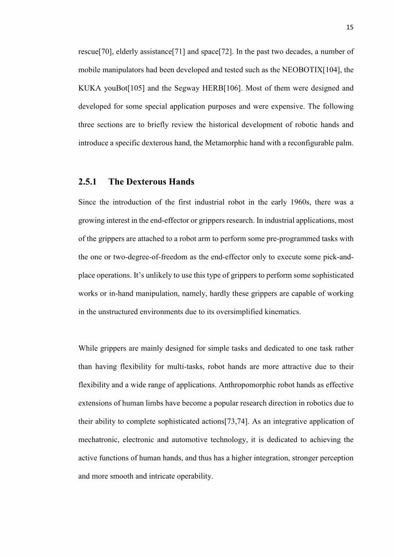
rescue[70], elderly assistance[71] and space[72]. In the past two decades, a number of
mobile manipulators had been developed and tested such as the NEOBOTIX[104], the
KUKA youBot[105] and the Segway HERB[106]. Most of them were designed and
developed for some special application purposes and were expensive. The following
three sections are to briefly review the historical development of robotic hands and
introduce a specific dexterous hand, the Metamorphic hand with a reconfigurable palm.
2.5.1 The Dexterous Hands
Since the introduction of the first industrial robot in the early 1960s, there was a
growing interest in the end-effector or grippers research. In industrial applications, most
of the grippers are attached to a robot arm to perform some pre-programmed tasks with
the one or two-degree-of-freedom as the end-effector only to execute some pick-and-
place operations. It’s unlikely to use this type of grippers to perform some sophisticated
works or in-hand manipulation, namely, hardly these grippers are capable of working
in the unstructured environments due to its oversimplified kinematics.
While grippers are mainly designed for simple tasks and dedicated to one task rather
than having flexibility for multi-tasks, robot hands are more attractive due to their
flexibility and a wide range of applications. Anthropomorphic robot hands as effective
extensions of human limbs have become a popular research direction in robotics due to
their ability to complete sophisticated actions[73,74]. As an integrative application of
mechatronic, electronic and automotive technology, it is dedicated to achieving the
active functions of human hands, and thus has a higher integration, stronger perception
and more smooth and intricate operability.
16
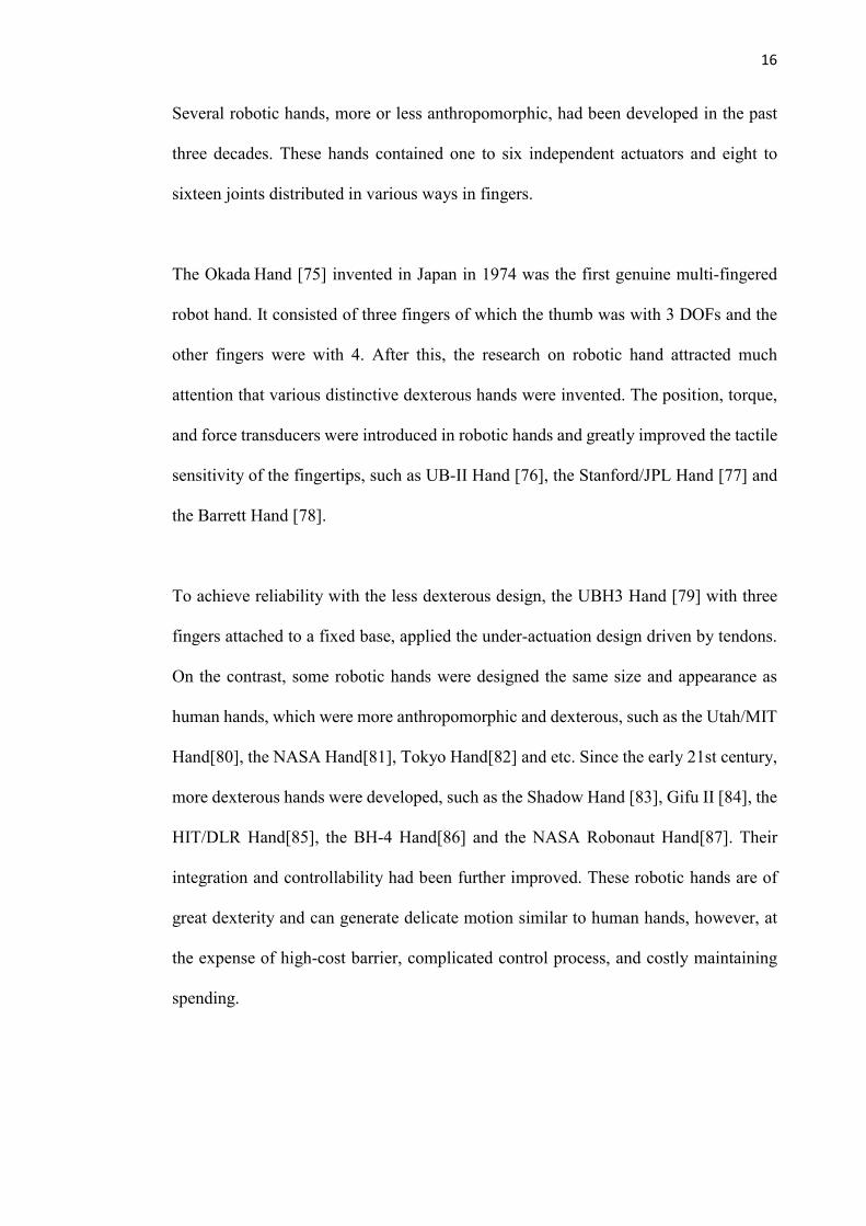
Several robotic hands, more or less anthropomorphic, had been developed in the past
three decades. These hands contained one to six independent actuators and eight to
sixteen joints distributed in various ways in fingers.
The Okada Hand [75] invented in Japan in 1974 was the first genuine multi-fingered
robot hand. It consisted of three fingers of which the thumb was with 3 DOFs and the
other fingers were with 4. After this, the research on robotic hand attracted much
attention that various distinctive dexterous hands were invented. The position, torque,
and force transducers were introduced in robotic hands and greatly improved the tactile
sensitivity of the fingertips, such as UB-II Hand [76], the Stanford/JPL Hand [77] and
the Barrett Hand [78].
To achieve reliability with the less dexterous design, the UBH3 Hand [79] with three
fingers attached to a fixed base, applied the under-actuation design driven by tendons.
On the contrast, some robotic hands were designed the same size and appearance as
human hands, which were more anthropomorphic and dexterous, such as the Utah/MIT
Hand[80], the NASA Hand[81], Tokyo Hand[82] and etc. Since the early 21st century,
more dexterous hands were developed, such as the Shadow Hand [83], Gifu II [84], the
HIT/DLR Hand[85], the BH-4 Hand[86] and the NASA Robonaut Hand[87]. Their
integration and controllability had been further improved. These robotic hands are of
great dexterity and can generate delicate motion similar to human hands, however, at
the expense of high-cost barrier, complicated control process, and costly maintaining
spending.

17
2.5.2 Dexterous Hands with a Reconfigurable Palm
In the development of dexterous hands, most researchers emphasized improving their
manipulability and dexterity by increasing finger numbers and finger joints or by
changing the structure of the thumb. Apart from flection in a plane, human fingers are
able to move in space as a result of the adduction/abduction motion achieved by the
Metacarpophalangeal (MCP) joint, which is analogous to the revolute-hook joint in its
kinematics equivalent. The finger adduction/abduction motion lays the foundation for
dextrous manipulation or in-hand manipulation with the capability of repositioning and
reorienting objects, which is the main gap of the robotic hands in contrast to human
hands. The adduction/abduction is a critical criterion to distinguish the dexterous
robotic hands and the lower-mobility robotic hands. In comparison to human hands
with a foldable and flexible palm, the most common robotic anthropomorphic hands
are less dexterous.
In particular, with the conventional design of mounting fingers to a rigid palm, a
conventional robotic hand cannot adapt to differences in the geometric shapes, which
limits the fine-tuning ability [88] and consequently the use of the robotic hand in object
grasping and handling. Since a typical robotic hand comprises of a palm and several
digits, it is worth noting that, rather than as a rigid holder to contain motors or
electronics, the palm with variable geometry can significantly enhance the dexterity of
the fingers mounted on it, resulting in augmenting the grasping and manipulation
capabilities of the robotic hand. The topology of the hand revamps comparing to
conventional robotic hands with an inflexible palm. For instance, BarrettTM [89]
presented a hand with three fingers rotating about the rigid palm driven by geared
system. Shadow [90] produced an anthropomorphic hand that splits the palm into two

18
halves with a larger thumb portion. As the palm parameters have a significant impact
on the finger workspace, making the palm reconfigurable establishes a new way to
design a robotic hand with relative low control complexity and acceptable dexterity.
2.5.3 The Metamorphic Hands
In most unconstructed environments the versatility of the palm is essential for
successful grasping and handling. This led to the introduction of the metamorphic
robotic hand [91,92], marking a turning point in improving dexterity and manipulability
of robotic hands. Metamorphosis is a term from biology meaning the evolution and
change of shapes and structure. Under the principle of Metamorphosis, the palm design
was inspired by origami with a mechanism equivalent method to relate the panels and
crisis to links and joints, respectively. An origami, in generous, has considerable
foldability that its geometry varies in a large ratio before and after folding. This
characteristic as the main advantage can be migrated to the robotic palm design in a
way to alter the workspace of the fingers to adjust the contact points with an object or
reposition or reorient an object during a manipulation. The foldable palm that extends
the kinematics chain of the fingers can liberate the latter from its motion plane to
generate spatial motion analogous to the adduction/abduction motion of the MCP joint
of human hands.
The Metamorphic hand broke the barrier by adopting a spherical metamorphic
mechanism, leading to a three-fingered robotic hand called Metahand with a
reconfigurable palm [93]. The metamorphic palm contributed to mimicking motions of
human hands, whose motion depended on both fingers and palm movements. A
significant amount of work had been carried out on the analysis of the palm’s motion
19
characteristics, geometric constraint, and palm workspace[60,61]. Dai et al. studied the
whole hand and demonstrated how the metamorphic palm affected the posture,
dexterity and workspace of the fingers[92,94,95] The metamorphic hand was
programmed to accomplish several grasps for objects widely used in our daily life with
different geometric features such as balls, bottles, and scissors, etc. [96]. A four-
fingered metamorphic hand was developed in light of the optimization of the five-
fingered Metamorphic hand applied to deboning operations [98].
2.5.4 Grasping Affordance
Grasping is one of the fundamental issues in robotic manipulation and different
concepts and principles have been introduced for grasp investigation. In cognitive
robotics, the concept of affordances [98] characterizes the relations between an agent
and its environment through the effects of the agent’s actions on the environment.
Affordances have become a popular formalization for autonomous manipulation
processes, bringing valuable insight into how manipulation can be done. Using the
concept of affordance, Detry et al. [99] modelled grasp affordances with continuous
probability density functions linking object-relative grasp poses to their success grasp
probability. Song et al. [100] developed a general framework for estimating grasp
affordances from 2-D sources combining texture-based and object level monocular
appearance cues for grasp affordance estimation.
Considering the flexible manipulator proposed in this work, by integrating the 3D
model of the three-fingered metamorphic robotic hand into the object-based grasp
affordance model [101] poses of the reference frame of the robotic hand can be
predicted providing a configuration for possible successful grasp. And with the poses
20
of the reference frame of the robotic hand given, locating the proposed mobile
manipulator becomes a problem of solving the inverse kinematics of the arm-wrist set
of the manipulator with the mobile platform at the range of the desired task position.
2.6 Conclusions
This chapter introduced the discovery of line geometry and line coordinates, and then
led to the introduction to screw algebra and screw coordinates, as well as the
construction of the ray coordinates and axis coordinates by Grassmann determinant
principle. Following this prior knowledge, twist and wrench were introduced by
extending screw theory to the mechanics and mechanisms with given physical meaning.
This chapter also presented the methodologies on the analysis of first-order kinematics
of a robot, particularly the screw-based method and derivative method. The
development of typical parallel mechanism and low-mobility parallel mechanisms was
also presented. Construction of a parallel mechanism was emphasized, with inspiration
from the multifingered hand grasping an object, a novel parallel mechanism was
proposed.
Moreover, state-of-the-art in the development of multifingered hands was introduced
with several well-known dexterous hands, followed by the latest improvement on hand
design by introducing a flexible palm to construct a Metamorphic hand. Hence the
motion of fingers in the Metamorphic hand depends on the palm geometry variation
that awards fingers the additional capability to move in space in such a way to enhance
the performance in comparison to the conventional three-fingered, rigid-palm hand.
21
State-of-the-art in the research of grasping affordance was also presented with the
application of the Metamorphic Hand.
22
Chapter 3 Geometry of Screw Coordinates
3.1 Introduction
Line geometry is a foundation for screw theory. A line in space can be presented with
homogeneous coordinates, which are extended by Plücker to ray coordinates and axis
coordinates, namely a line as a ray between two points and a line as the intersection of
two planes. Ray coordinates, or Plücker coordinates in ray order, are made up of the
first three components as the primary part that presents the direction of a line and the
last three components as the secondary part implicitly gives the location of the line with
the moment of the line with respect to the origin. Axis coordinates, or Plücker
coordinates in axis order have the first three components as the moment of the line and
the last three components indicating the direction of the line.
In this chapter, in order to make a geometrical presentation to reveal the insight in
Euclidean 3-space, that is a three-dimensional real vector space that preserves the
Euclidean metric, homogeneous coordinates of a point and a plane are converting to a
set of homogeneous coordinates with the last component as 1, using ratios of
homogeneous coordinates. Accordingly, we shall use this set of homogeneous
coordinates and non-homogeneous coordinates side by side, passing from one to the
other when it is in line with the derivation with ratio sign/colon to separate components
while in homogeneous coordinates.
23
3.2 Position Vectors and Their Triangular Resultant for
Ray Coordinates
Homogeneous coordinates of points P1 and P2 might be presented as r’1=(x’
1: y’1: z’
1:
w1)T and r’2=(x’
2: y’2: z’
2: w2)T which could be represented with ratios of these four
components, namely dividing each by the last component w. Without loss of generality,
placing w1=w2=1, the homogeneous coordinates can be converted to a set of
homogeneous coordinates as r’1=(x1: y1: z1: 1)T and r’
2=(x2: y2: z2: 1)T as the
homogeneous representation for points P1 and P2 in the form of position vectors r1=(x1,
y1, z1)T and r2=(x2, y2, z2)T in their non-homogeneous coordinates. In Euclidean 3-space,
we may think of its elements as vectors [30] in a three-dimensional real vector space
that preserves the Euclidean metric. These two points that define a straight line in Fig.
3.1 as joint of points can be expressed as position vectors r1 and r2. This gives the
direction vector of a line as the primary part of line vector L=(lT; l0T) in the form of
( )T
2 1 , ,l m n- =l = r r . (3.1)
Figure 3.1 A line with two position vectors
24
Projecting the line onto a plane parallel to x-y plane with its projection angle and
further projecting its projection to x-axis with projection angle , the x-axis component
l can be expressed as the function of these two angles and rearranged as a 2´2 minor
that is coined as a determinant by Grassmann expansion [31] as follows,
1
2 1
2
1cos cos
1
xl x x
x = = - =l . (3.2)
Similarly, projections of the direction of the line on two remaining coordinate axes can
be written as the function of projection angles and and expressed as 2´2 minors in
the form of
1
2 1
2
1cos sin
1
ym y y
y = = - =l , (3.3)
1
2 1
2
1sin
1
zn z z
z= = - =l . (3.4)
This gives three components as the primary part l of line vector L and is represented as
three projections l, m and n in Fig. 3.2. The moment of this vector with respect to the
origin can be obtained by taking moment of the direction vector l with respect to each
of the coordinate axes and gives the secondary part l0=(p, q, r)T of line vector L.
25
Figure 3.2 Geometrical interpretation of Plücker coordinates in ray order of a line
Moment component p of the direction vector l with respect to coordinate axis x might
be obtained as
2 2sin cos sinp y z = -l l .
Substituting Eqs. (3.3) and (3.4) in the above gives the following expression that is
rearranged as a 2´2 minor in the form of
( ) ( ) 1 1
2 1 2 2 1 2 1 2 2 1
2 2
y z
p z z y y y z y z y zy z
= - - - = - = . (3.5)
Similarly, moment components q and r can be obtained by taking moment of the
direction vector l with respect to coordinate axes y and z, and substituting Eqs. (3.2) to
(3.4) for replacing functions of angles and as follows,
26
( ) ( )
2 2
1 1
2 1 2 2 1 2 2 1 1 2
2 2
cos cos sinq z x
z xx x z z z x x z x z
z x
= -
= - - - = - =
l l
, (3.6)
( ) ( )
2 2
1 1
2 1 2 2 1 2 1 2 2 1
2 2
cos sin cos cosr x y
x yy y x x x y x y x y
x y
= -
= - - - = - =
l l
. (3.7)
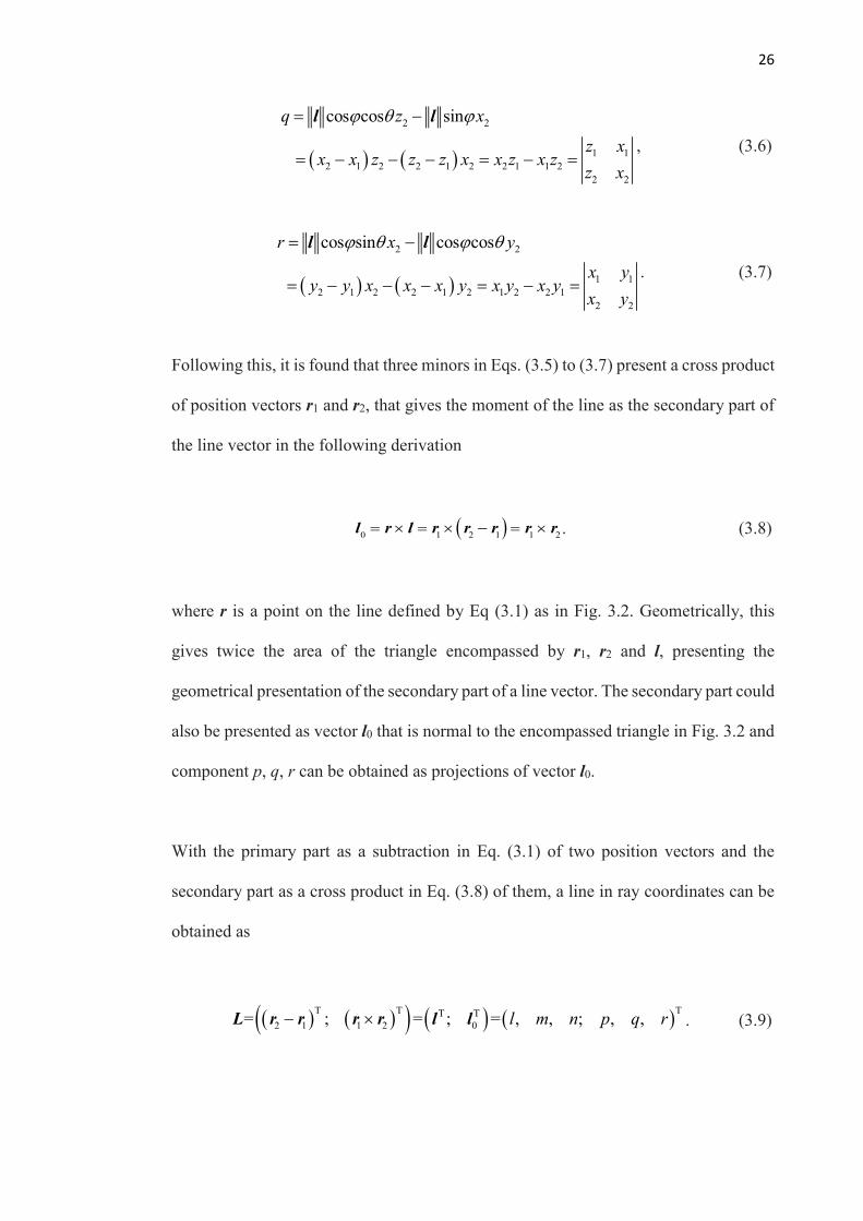
Following this, it is found that three minors in Eqs. (3.5) to (3.7) present a cross product
of position vectors r1 and r2, that gives the moment of the line as the secondary part of
the line vector in the following derivation
l
0= r ´ l = r
1´ r
2- r
1( ) = r1´ r
2 . (3.8)
where r is a point on the line defined by Eq (3.1) as in Fig. 3.2. Geometrically, this
gives twice the area of the triangle encompassed by r1, r2 and l, presenting the
geometrical presentation of the secondary part of a line vector. The secondary part could
also be presented as vector l0 that is normal to the encompassed triangle in Fig. 3.2 and
component p, q, r can be obtained as projections of vector l0.
With the primary part as a subtraction in Eq. (3.1) of two position vectors and the
secondary part as a cross product in Eq. (3.8) of them, a line in ray coordinates can be
obtained as
( ) ( )( ) ( ) ( )T T TT T
2 1 1 2 0= ; = ; = , , ; , ,l m n p q r- ´L r r r r l l . (3.9)

27
The geometrical meaning can be revealed in Fig. 3.2 with the primary part as a side of
the triangle constructed by position vectors r1 and r2 and the secondary part as a normal
of the triangle. In a special case, if a line is passing the origin, Eq (3.9) becomes
L=( ( )T T
2 1 ;- 0r r ). The six distinct 2´2 minors from Grassmann expansion in Eqs.
(3.2) to (3.7) can be summarized as follows by two position vectors in their
homogeneous coordinates as
x
1y
1z
11
x2
y2
z2
1
. (3.10)
3.3 Projected Triangle for Axis Coordinates with Weighted
Plane Normals
3.3.1 Duality in Point-Plane Representations of a Line
Dual to the above of presenting a line as a ray of two points, a line in space can be
presented as an intersection of two planes in Fig. 3 to form a system of linear equations.
Plane coordinates of these two intersecting planes in homogeneous coordinates can be
presented as ( )' ' ' '1 1 1 1: : :A B C D and ( )' ' ' '
2 2 2 2: : :A B C D . In this
representation, the first three components are the normals of planes 1 and 2 and the
last component gives the distance from the origin to each of the planes. Taking ratios
of four components of the plane coordinates above as coordinates of two vectors, two
weighted plane normal can be presented in homogenous coordinates with the last
component as 1 as ( )T'
1 1 1 1: : : 1A B C=n and ( )T'
2 2 2 2: : : 1A B C=n , where
A1, B1, and C1 are obtained by dividing the distance D1´ of plane 1 and A2, B2, and C2

28
are obtained by dividing the distance D2´ of plane 2. This representation covers all lines
except for lines passing the origin. When lines pass the origin, the case will be discussed
in the duality and conformability section.
This gives the following weighted plane normals in the three-dimensional space
( )
( )
T
1 1 1 1
T
2 2 2 2
, ,
, ,
A B C
A B C
=
=
n
n. (3.11)
Figure 3.3 A line as the intersection of two planes
Selecting point r=(x: y: z: 1)T along the intersection of two planes in its homogeneous
representation with the last component as 1, the line as the intersection of two planes
can be presented as follows
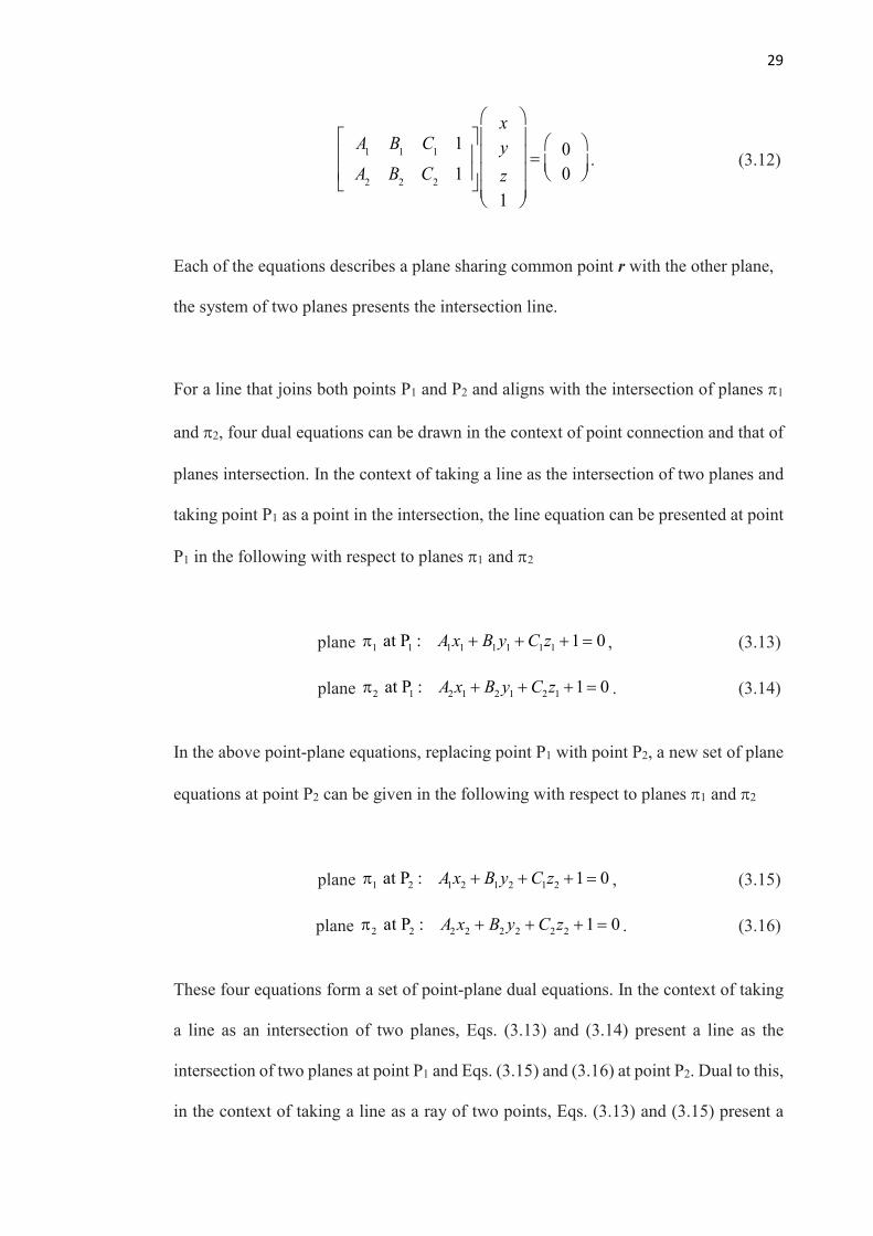
29
A
1B
1C
11
A2
B2
C2
1
x
y
z
1
= 0
0
. (3.12)
Each of the equations describes a plane sharing common point r with the other plane,
the system of two planes presents the intersection line.
For a line that joins both points P1 and P2 and aligns with the intersection of planes 1
and 2, four dual equations can be drawn in the context of point connection and that of
planes intersection. In the context of taking a line as the intersection of two planes and
taking point P1 as a point in the intersection, the line equation can be presented at point
P1 in the following with respect to planes 1 and 2
plane 1 11 1 1 1 1 1 at P : 1 0A x B y C z + + + = , (3.13)
plane 2 2 1 2 1 2 11 at P : 1 0A x B y C z + + + = . (3.14)
In the above point-plane equations, replacing point P1 with point P2, a new set of plane
equations at point P2 can be given in the following with respect to planes 1 and 2
plane 2 1 2 1 2 1 21 at P : 1 0A x B y C z + + + = , (3.15)
plane 2 2 2 2 2 2 2 2 at P : 1 0A x B y C z + + + = . (3.16)
These four equations form a set of point-plane dual equations. In the context of taking
a line as an intersection of two planes, Eqs. (3.13) and (3.14) present a line as the
intersection of two planes at point P1 and Eqs. (3.15) and (3.16) at point P2. Dual to this,
in the context of taking a line as a ray of two points, Eqs. (3.13) and (3.15) present a
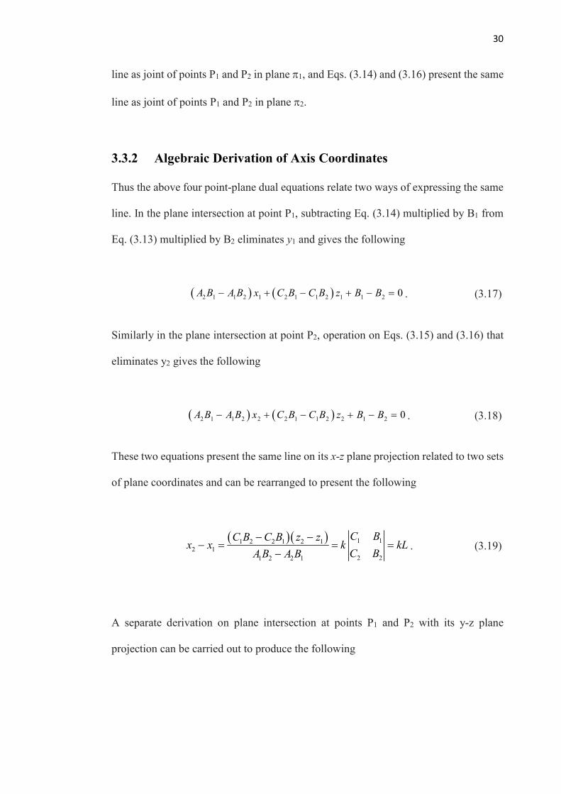
30
line as joint of points P1 and P2 in plane 1, and Eqs. (3.14) and (3.16) present the same
line as joint of points P1 and P2 in plane 2.
3.3.2 Algebraic Derivation of Axis Coordinates
Thus the above four point-plane dual equations relate two ways of expressing the same
line. In the plane intersection at point P1, subtracting Eq. (3.14) multiplied by B1 from
Eq. (3.13) multiplied by B2 eliminates y1 and gives the following
( ) ( )2 1 1 2 1 2 1 1 2 1 1 2 0A B A B x C B C B z B B- + - + - = . (3.17)
Similarly in the plane intersection at point P2, operation on Eqs. (3.15) and (3.16) that
eliminates y2 gives the following
( ) ( )2 1 1 2 2 2 1 1 2 2 1 2 0A B A B x C B C B z B B- + - + - = . (3.18)
These two equations present the same line on its x-z plane projection related to two sets
of plane coordinates and can be rearranged to present the following
( ) ( ) 1 11 2 2 1 2 1
2 1
2 21 2 2 1
C BC B C B z zx x k kL
C BA B A B
- -- = = =
-. (3.19)
A separate derivation on plane intersection at points P1 and P2 with its y-z plane
projection can be carried out to produce the following
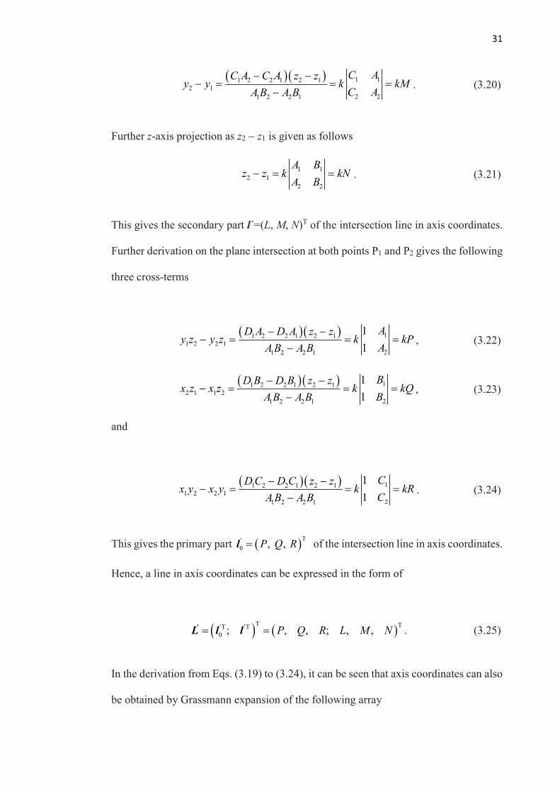
31
( ) ( ) 1 11 2 2 1 2 1
2 1
2 21 2 2 1
C AC A C A z zy y k kM
C AA B A B
- -- = = =
-. (3.20)
Further z-axis projection as z2 - z1 is given as follows
1 1
2 1
2 2
A Bz z k kN
A B- = = . (3.21)
This gives the secondary part l´=(L, M, N)T of the intersection line in axis coordinates.
Further derivation on the plane intersection at both points P1 and P2 gives the following
three cross-terms
( ) ( ) 11 2 2 1 2 1
1 2 2 1
21 2 2 1
1
1
AD A D A z zy z y z k kP
AA B A B
- -- = = =
-, (3.22)
( ) ( ) 11 2 2 1 2 1
2 1 1 2
21 2 2 1
1
1
BD B D B z zx z x z k kQ
BA B A B
- -- = = =
-, (3.23)
and
( ) ( ) 11 2 2 1 2 1
1 2 2 1
21 2 2 1
1
1
CD C D C z zx y x y k kR
CA B A B
- -- = = =
-. (3.24)
This gives the primary part ( )T'
0 , , P Q R=l of the intersection line in axis coordinates.
Hence, a line in axis coordinates can be expressed in the form of
( ) ( )T T'T 'T
0 ; , , ; , ,P Q R L M N= ='L l l . (3.25)
In the derivation from Eqs. (3.19) to (3.24), it can be seen that axis coordinates can also
be obtained by Grassmann expansion of the following array

32
A1
B1
C1
1
A2
B2
C2
1
. (3.26)
where (A1, B1, C1) is weighted plane normal n1 and (A2, B2, C2) is weighted plane normal
n2 in the three-dimensional space.
3.3.3 Geometrical Presentation of Axis Coordinates
In the six axis coordinates obtained from Eqs. (3.19) to (3.24), it can be seen that
components L, M, N in Eqs. (3.19) to (3.21) as the secondary part of the line vector are
the result of the cross product of weighted plane normals n1 and n2 of planes 1 and 2
in the form of
l ' = n1´ n
2=
i j k
A1
B1
C1
A2
B2
C2
=B
1C
1
B2
C2
i +C
1A
1
C2
A2
j +A
1B
1
A2
B2
k . (3.27)
This gives the direction vector of the intersection line L´ as in Eq. (3.25) and the
triangular presentation in Fig. 3.4 of this secondary part of a line in axis coordinates
with twice the area of the triangle encompassed by n1, n2 and as n2-n1. Consistent with
the secondary part of a line vector in Fig. 3.2 in ray coordinates in Eq. (3.9), it could
also be presented by vector l´ that is normal to the triangle in Fig. 3.4.
33
Figure 3.4 Geometrical interpretation of the axis coordinates
To reveal the geometrical meaning of the primary part components P, Q, R of axis
coordinates obtained in Eqs. (3.22) to (3.24), assigning z=0 in Eq. (3.12) of the
intersection line of two planes, the following can be provided
1 1 1 0A x B y+ + = , (3.28)
2 2 1 0A x B y+ + = . (3.29)
The position vector for the intersection line can be obtained as,
T
2 1 1 2
2 1 1 2 2 1 1 2
, , 0g
B B A A
A B A B A B A B
- -=
- - r . (3.30)
Hence the moment of the intersection line with respect to the origin is given in the form
of
34
l0
' = r ´ l ' = rg´ l ' = A
2- A
1, B
2- B
1, C
2-C
1( )T
= n2- n
1. (3.31)
This gives three components P, Q, R as the primary part of the intersection line in axis
coordinates in the form of weighted plane normals. Therefore, this presents vector
'2 1 0- =n n l in Fig. 3.4 whose projections give three components P, Q, R as the primary
part of the intersection line, in a geometrical presentation consistent with projections of
2 1- =r r l in Fig. 3.2 of the primary part of a line vector in ray coordinates.
The geometrical meaning of the primary part in axis coordinates is hence given as a
subtraction of two weighted plane normal, consistent with the mathematical structure
of the primary part l of the ray coordinates expressed in Eqs. (3.2) to (3.4).
Similarly, the secondary part in axis coordinates is consistent with the mathematical
structure in the secondary part of ray coordinates. In these two sets of coordinates, the
primary part and secondary part are constructed by position vectors in ray coordinates
and by weighted plane normals in axis coordinates.
The geometrical meaning can hence be revealed in Fig. 3.4 with the primary part '0l as
a side of a triangle constructed by two weighted plane normal and the secondary part l
as a normal of the triangle.
3.4 Conclusions
This chapter revealed the geometrical presentation of a line as a ray of two points in the
form of position vectors with their triangle presentation and derived the geometrical
35
presentation of a line as an intersection of two planes in the form of plane normals with
another triangle presentation, giving a line in its ray coordinates and axis coordinates.
In particular, it was verified for the first time the secondary part (L, M, N) in axis
coordinates as the cross product of weighted plane normals of the intersection planes
and the primary part (P, Q, R) in axis coordinates as the vector subtraction of the
weighted plane normals.

36
Chapter 4 Geometrically Intrinsic
Connections of Screw Coordinates
4.1 Introduction
This chapter reveals the geometrical insight of ray coordinates with twice the area
projection in a triangle constructed by two position vectors and presents the geometrical
meaning of the axis coordinates with the geometrical presentation for the first time
between two normals of the intersecting planes that give a corresponding triangle
constructed by these normals. This leads to a natural derivation of the ratio relationship
between ray and axis coordinates, and to a duality of these two sets of coordinates.
During the derivation, form conformability in the mathematical structures of
corresponding parts of two sets of coordinates is revealed, and geometrical
conformability is identified in the reciprocal parts of these two sets of coordinates that
are presented in two vector spaces that are dual to each other. The study derives
naturally the correlation relationship with a correlation coefficient and the correlation
operator, leading to a duality and conformability table and a conformability graph.
4.2 Form and Geometry Conformability of Two Sets of
Coordinates
In the derivation of ray and axis coordinates, it can be seen that a triangle presentation
exists in either set of coordinates. The closing vector of the triangle is a subtraction of
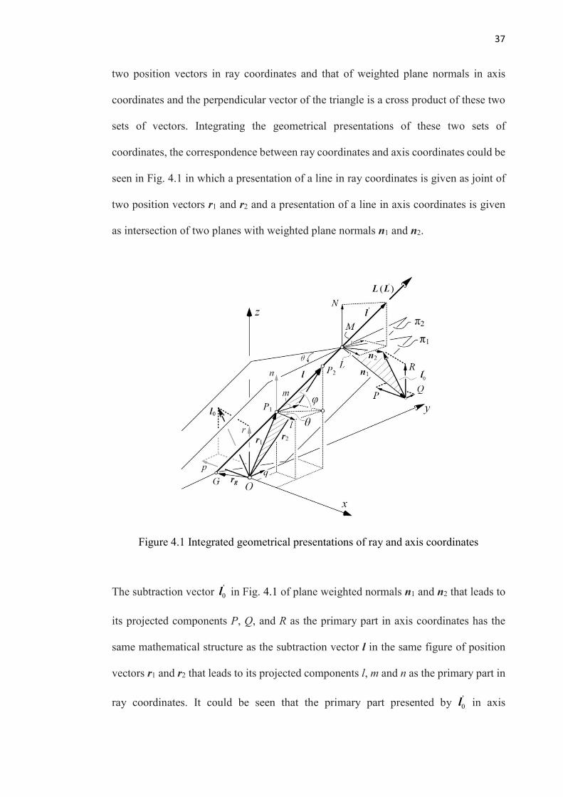
37
two position vectors in ray coordinates and that of weighted plane normals in axis
coordinates and the perpendicular vector of the triangle is a cross product of these two
sets of vectors. Integrating the geometrical presentations of these two sets of
coordinates, the correspondence between ray coordinates and axis coordinates could be
seen in Fig. 4.1 in which a presentation of a line in ray coordinates is given as joint of
two position vectors r1 and r2 and a presentation of a line in axis coordinates is given
as intersection of two planes with weighted plane normals n1 and n2.
Figure 4.1 Integrated geometrical presentations of ray and axis coordinates
The subtraction vector '0l in Fig. 4.1 of plane weighted normals n1 and n2 that leads to
its projected components P, Q, and R as the primary part in axis coordinates has the
same mathematical structure as the subtraction vector l in the same figure of position
vectors r1 and r2 that leads to its projected components l, m and n as the primary part in
ray coordinates. It could be seen that the primary part presented by '0l in axis
38
coordinates is consistent with the primary part presented by l in ray coordinates in the
sense of form conformability. Further, the primary part '0l in axis coordinates has the
same geometrical meaning as the secondary part l0=r1´r2 in ray coordinates as the
moment of the line in the sense of geometry conformability. In such a case, they have
the same direction as in Fig. 4.1 that
l0= kl
0
' , (4.1)
where k will be discussed in Section 4.4.
The secondary part l´=n1´n2 of axis coordinates with its components L, M and N
represented by the normal of the triangle constructed by n1 and n2 in Fig. 4.1 has the
same mathematical structure as the secondary part l0=r1´r2 of ray coordinates with its
components p, q, and r represented by the normal of the triangle constructed by r1 and
r2 in the same figure. This gives form conformability. Further, the secondary part l´ of
axis coordinates has the same geometrical meaning as the primary part l in ray
coordinates of the direction of the line in the sense of geometry conformability. In such
a case, they are on the same line as in Fig. 4.1 that
l = kl ' , (4.2)
where k will be discussed in Section 4.4.
As demonstrated, a line vector as joint of two points in space is dual to a line vector as
the intersection of two planes, in the way of ray coordinates dual to axis coordinates.

39
Placing the former in the vector space and the latter in the dual vector space, their
duality is clearly illustrated in the following sections. As such, the coordinates can be
mapped onto one another as in the correlation equation in the following section.
4.3 Correlated Ratio Relationships
Duality of a line in its ray and axis coordinates represented by point-plane dual
equations (3.13) to (3.16) leads to the correlated ratio relationship between the
corresponding primary and secondary parts of ray and axis coordinates that can be
derived from the following. Starting from point-plane dual equations Eqs (3.13) and
(3.14), it results in
( ) ( ) ( )1 2 1 1 2 1 1 2 1 0A A x B B y C C z- + - + - = . (4.3)
It can be easily seen that the components in the parentheses are axis coordinates P, Q,
R expressed in Eqs. (3.22) to (3.24), the above equation can then be rewritten as
1 1 1 0Px Qy Rz+ + = . (4.4)
This gives the primary part of axis coordinates in relation to point P1 given by position
vector r1. Similarly, from another set of point-plane dual equations Eqs. (3.15) and
(3.16), the following can be derived
2 2 2 0Px Qy Rz+ + = . (4.5)

40
This gives the primary part of axis coordinates in relation to point P2 given by position
vector r2. Subtracting Eq. (4.5) that is multiplied by y1 from Eq. (4.4) that is multiplied
by y2, gives the following
( ) ( )1 2 2 1 2 1 1 2 0P x y x y R y z y z- + - = . (4.6)
It is clear that the components in the parentheses are secondary part p and r of ray
coordinates as in Eqs. (3.5) and (3.7) and this gives a relationship between the
secondary part of ray coordinates and the primary part of axis coordinates. Substituting
p and r of ray coordinates in Eqs. (3.5) and (3.7) for the components in the parentheses
in the above equation and rearranging it, the following is given
1 2 2 1
1 2 2 1
P y z y z p
R x y x y r
-= =
-. (4.7)
In a way similar to the above process that generates Eq. (4.7), subtracting Eq. (4.5) that
is multiplied by x1 from Eq. (4.5) that is multiplied by x2 and substituting q and r in
Eqs. (3.6) and (3.7) of ray coordinates for the components in the parentheses, the
following is given
2 1 1 2
1 2 2 1
Q x z x z q
R x y x y r
-= =
-. (4.8)
Thus from Eqs. (4.7) and (4.8), the following part correlated ratio relationship of the
primary part of axis coordinates with respect to the secondary part of ray coordinates
can be given
41
P : Q : R = p : q : r . (4.9)
This gives the P part correlated ratio relationship of ray and axis coordinates.
The relationship of the secondary part of axis coordinates and the primary part of ray
coordinates can be given following the similar derivation in point-plane dual equations
Eqs. (3.13) and (3.15). Eqs. (3.13) and (3.15) present a line as joint of two points in
plane 1 with components in the parentheses as the secondary part of the line in axis
coordinates in Eqs. (3.19) to (3.21), the primary part of ray coordinates of the line can
be written in terms of plane coordinates of plane 1 that form the secondary part of axis
coordinates. In a similar way, the primary part of ray coordinates of the line can be
written in terms of plane coordinates of plane 2 that form the secondary part of axis
coordinates. These two relations can be rearranged by substituting for the components
in the parentheses with the secondary part of axis coordinates from Eqs. (3.19) to (3.21),
yielding the following L part relationship
L : M : N = l : m : n . (4.10)
Hence, both L part and P part ratio relationships are obtained. To associate these two
correlated ratio relationships, a L-P cross-part ratio relationship needs to be obtained.
In the context of a line as the intersection of planes 1 and 2 at point P1 in Eqs. (3.13)
and (3.14) and as the intersection of planes 1 and 2 at point P2 in Eqs. (3.15) and
(3.16), manipulation of these equations together with the substitution by axis
coordinates between Eqs. (3.19) and (3.22) gives the following cross-part relationship,
L : P = l : p . (4.11)
42
Hence, two sets of L part ratio and P part ratio relationships can be associated with the
above L-P cross-part ratio between ray and axis coordinates. The part correlated ratio
relationship in Eqs. (4.9) and (4.10) and the cross-part correlated ratio relationship in
Eq. (4.11) present duality of ray and axis coordinates and can be rearranged to generate
the following relationship in the form of
L : M : N : P : Q : R = l : m : n : p : q : r . (4.12)
The above can be rewritten as
l : L = m : M = n : N = p : P = q : Q = r : R = k . (4.13)
The above derivation reveals duality between ray and axis coordinates and presents a
correlation coefficient k.
4.4 Correlation Coefficient and Correlation Operator
Consistent with the above ratio relationship, observing ray coordinates equations from
Eqs. (3.2) to (3.7), it can be seen that the left-hand sides of Eqs. (3.19) to (3.21) in
Section 3.2 give the direction vector l=(l, m, n)T in ray coordinates while the right-hand
sides give the secondary part ( )T'
0 , , L M N=l in axis coordinates of a line vector, the
left-hand sides of Eqs (3.22) to (3.24) in Section 3.3.2 give the moment l0=(p, q, r)T in
ray coordinates while the right-hand sides give the primary part ( )T' , , P Q R=l in axis
coordinates of the line vector. This leads to the following correlation between two sets
of coordinates,

43
( )
( )
( )
( )
T
T
2 1 2 1 2 1 1 2 2 1 2 1 1 2 1 2 2 1
T
1 2 2 1 1 2 2 1 1 2 2 1 2 1 2 1 2 1
T '
, , ; , ,
, , ; , ,
, , ; , ,
, , ; , ,
l m n p q r
x x y y z z y z y z x z x z x y x y
k C B C B C A C A A B A B A A B B C C
k L M N P Q R k
=
= - - - - - -
= - - - - - -
= = D
L
L
(4.14)
giving rise naturally to use the following correlation operator,
D =
0
0
I
I, (4.15)
and the correlation coefficient as
k =z
2- z
1
A1B
2- A
2B
1
=n
N. (4.16)
It again can be seen that this correlation coefficient k is a ratio between two sets of
coordinates that is given in Eq (4.13) and is invariant.
Considering points P1 and P2 being distinct with at least one of the three coordinates
distinct, Eq. (4.14) gives the correlation between ray coordinates L and axis coordinates
L´ when presenting the same line.
As six coordinates provide ratios as in Eq (4.12) in homogeneous coordinates, the
magnitude change of a line vector does not change itself. Hence, without loss of
generality, k can be assigned with 1 and the correlation equation (4.14) can be
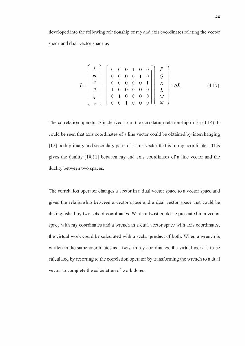
44
developed into the following relationship of ray and axis coordinates relating the vector
space and dual vector space as
L =
l
m
n
p
q
r
=
0 0 0 1 0 0
0 0 0 0 1 0
0 0 0 0 0 1
1 0 0 0 0 0
0 1 0 0 0 0
0 0 1 0 0 0
P
Q
R
L
M
N
= DL' . (4.17)
The correlation operator D is derived from the correlation relationship in Eq (4.14). It
could be seen that axis coordinates of a line vector could be obtained by interchanging
[12] both primary and secondary parts of a line vector that is in ray coordinates. This
gives the duality [10,31] between ray and axis coordinates of a line vector and the
duality between two spaces.
The correlation operator changes a vector in a dual vector space to a vector space and
gives the relationship between a vector space and a dual vector space that could be
distinguished by two sets of coordinates. While a twist could be presented in a vector
space with ray coordinates and a wrench in a dual vector space with axis coordinates,
the virtual work could be calculated with a scalar product of both. When a wrench is
written in the same coordinates as a twist in ray coordinates, the virtual work is to be
calculated by resorting to the correlation operator by transforming the wrench to a dual
vector to complete the calculation of work done.
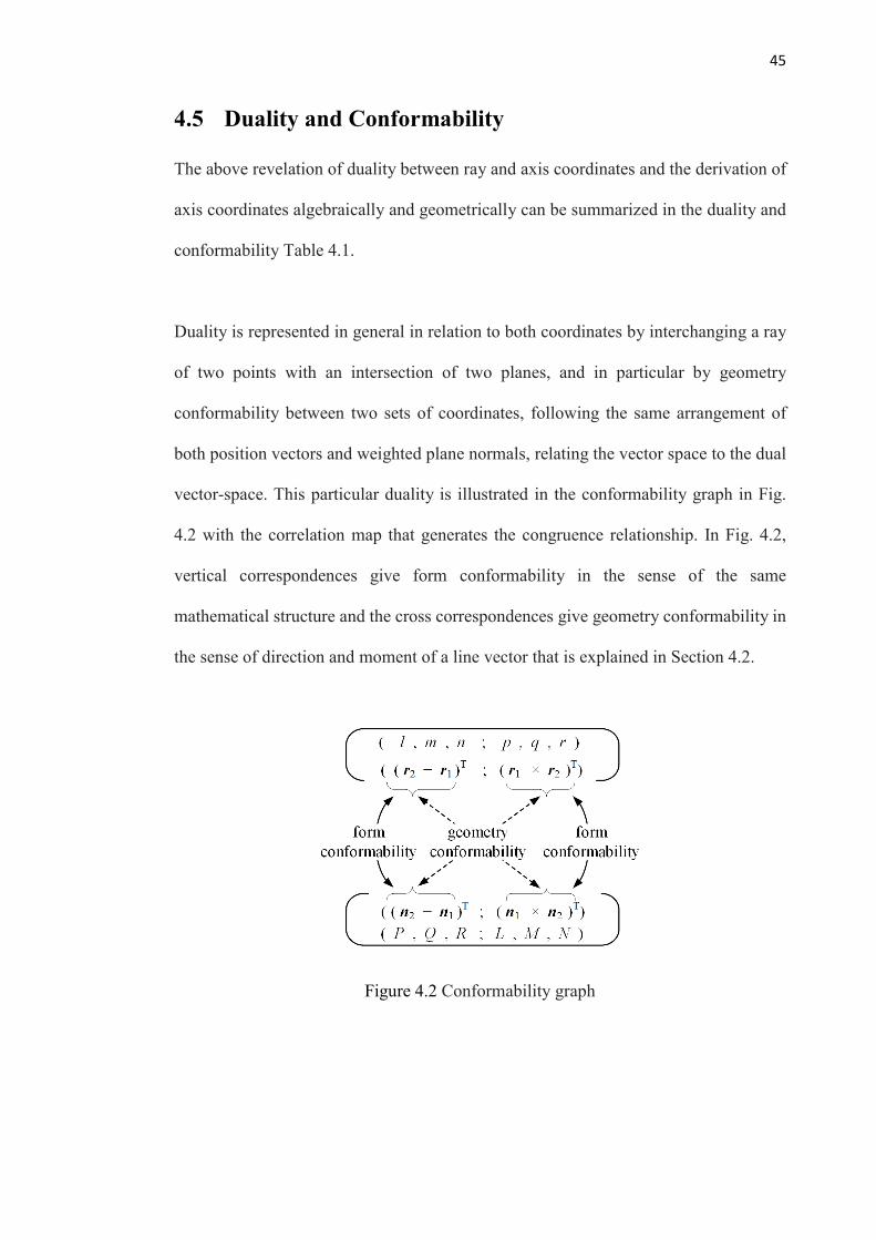
45
4.5 Duality and Conformability
The above revelation of duality between ray and axis coordinates and the derivation of
axis coordinates algebraically and geometrically can be summarized in the duality and
conformability Table 4.1.
Duality is represented in general in relation to both coordinates by interchanging a ray
of two points with an intersection of two planes, and in particular by geometry
conformability between two sets of coordinates, following the same arrangement of
both position vectors and weighted plane normals, relating the vector space to the dual
vector-space. This particular duality is illustrated in the conformability graph in Fig.
4.2 with the correlation map that generates the congruence relationship. In Fig. 4.2,
vertical correspondences give form conformability in the sense of the same
mathematical structure and the cross correspondences give geometry conformability in
the sense of direction and moment of a line vector that is explained in Section 4.2.
Figure 4.2 Conformability graph
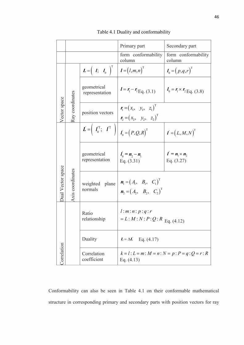
46
Table 4.1 Duality and conformability
Primary part Secondary part
form conformability column
form conformability column
Vec
tor
spac
e
Ray
coo
rdin
ates
L = l; l
0( )T
l = l,m,n( )
T
l0= p,q,r( )
T
geometrical representation l = r
1- r
1Eq. (3.1) l0= r
1´ r
2 Eq. (3.8)
position vectors ( )
T
1 1 1 1, ,x y z=r
( )T
2 2 2 2, ,x y z=r
Dua
l V
ecto
r sp
ace
Axi
s co
ordi
nate
s
L' = l0
'T; l 'T( )
l0
' = P,Q, R( )T
l ' = L, M , N( )
T
geometrical representation
l0
' = n2- n
1 Eq. (3.31)
'1 2´l = n n
Eq. (3.27)
weighted plane normals
( )T
1 1 1 1, ,A B C=n
( )T
2 2 2 2, ,A B C=n
Ratio relationship
: : : : :
: : : : :
l m n p q r
L M N P Q R= Eq. (4.12)
Cor
rela
tion
Duality L = DL' Eq. (4.17)
Correlation coefficient
k = l : L = m : M = n : N = p : P = q : Q = r : R Eq. (4.13)
Conformability can also be seen in Table 4.1 on their conformable mathematical
structure in corresponding primary and secondary parts with position vectors for ray
47
coordinates and weighted plane normals for axis coordinates. Parts in each column of
Table 4.1 are conformable in their mathematical structures as form conformability.
Duality and geometry conformability always coexist. But duality and form
conformability only coexist when there is no point in the infinity in the vector space
such as wi≠0 and there is no plane passing through the origin in the dual vector space
such as Di≠0.
While any scaling factor that is the last component in homogeneous coordinates is equal
to zero, duality and geometry conformability still coexist, but duality and form
conformability are disconnected. This can be seen that when a line is passing the origin
in ray coordinates as ((r2-r1)T; 0T) , its dual in axis coordinates is (0T; (n1´n2)T). As a
matter of interest, its form-conformable axis coordinates could be ((n2-n1)T; 0T) that
presents a line in the infinity. Vice versa, when a line is in the infinity in ray coordinates
as (0T; (r1×r2)T), its dual in axis coordinates is ((n2–n1)T; 0T). But as a matter of interest,
its form-conformable axis coordinates could be (0T; (n1×n2)T) that presents a line
passing the origin. In such an occasion, though duality and geometry conformability
always coexist, duality and form conformability no longer coexists.
4.6 Conclusions
In the derivation, it was found that the subtraction vector of two position vectors in ray
coordinates and that of two weighted plane normals in axis coordinates are a closing
vector of the triangle formed by two vectors in each coordinate set and the cross-product
vector was perpendicular to the triangle formed by these two vectors in each coordinate
set. Two presentations were related geometrically and algebraically and presented
48
conformability and duality between corresponding and reciprocal parts of ray and axis
coordinates, with an illustration presenting an integration of geometrical presentations
for both ray and axis coordinates in their form conformability and geometry
conformability.
In this chapter, the work was then extended to presenting a correlation between ray and
axis coordinates with their correlated part ratios to relate the vector space to the dual
vector space, and to deriving a correlation between two sets of coordinates with a
correlation coefficient, giving rise to a derivation of the correlation operator. The
duality was then recapitulated in a duality and conformability table and in a
conformability graph, outlining the relationship between ray and axis coordinates of a
line vector.
The study presented a geometrical and algebraic foundation for using line vectors in
their two sets of coordinates for mechanism analysis and synthesis.
49
Chapter 5 Geometrical Meaning of a Twist
Based on Screw Algebra
5.1 Introduction
Line geometry and line vectors, particularly the ray coordinates and axis coordinates
and their interrelation are well received in Chapters 3 and 4. By associating a line vector
with a pitch, a screw is formed. A screw is a geometrical entity, and is an element of
the projective Lie algebra se(3). The geometrical meaning of the pitch of a screw is the
ratio of the magnitude of the second component of the secondary part over that of the
primary part.
A twist is formed by attaching a screw with a velocity amplitude, and it is an element
of the Lie algebra se(3). The primary part of a twist indicates the angular velocity of a
rigid body, whereas the secondary part indicates the linear velocity of a point on this
rigid body instantaneously coincident with the reference point. The twists that represent
the instantaneous velocity of links in a serial manipulator can be assembled to generate
a resultant twist of the end-effector. Geometrical meaning of the resultant twist is
revealed in this chapter and the Jacobian of a planar serial manipulator is formed
through screw algebra.
50
5.2 Homogenous Coordinates of Screws as 6-Dimensional
Vector
5.2.1 Homogenous Screw Coordinates
A screw is essentially the geometrical entity of instantaneous twist and wrench in
kinematics and statics, which in general can be regarded as a line vector in 3-
dimensional affine space 3 together with pitch h. The screw can be expressed by dual
vector and 6-dimensional vector respectively as follows
0
0 0
= = =h
+ ´ +
s sS s s
s r s s. (5.1)
where the vector s is the primary part of the screw, representing the direction vector of
screw axis, the vector s0 is the secondary part of the screw that consists of the moment
with respect to the origin and the scalar product of the primary part by pitch h, the 3-
dimensional vector r0 represents the position vector of the screw axis with respect to
the origin and ε is dual unit of dual vector satisfying the condition ε2 = 0. The conception
of dual vector originally comes from dual number brought forward by Clifford (1876)
in his research on quaternions and extensively developed by Brand (1940) in his
exploration on motor algebra in which the screw is seen as dual vector called motor.
Obviously, screw as a geometrical entity can be described as a 6-dimensional vector,
that is to say, screw and 6-dimensional vector are equivalent so that all the operations
of screws can be performed in the form of vector operations and further by matrix
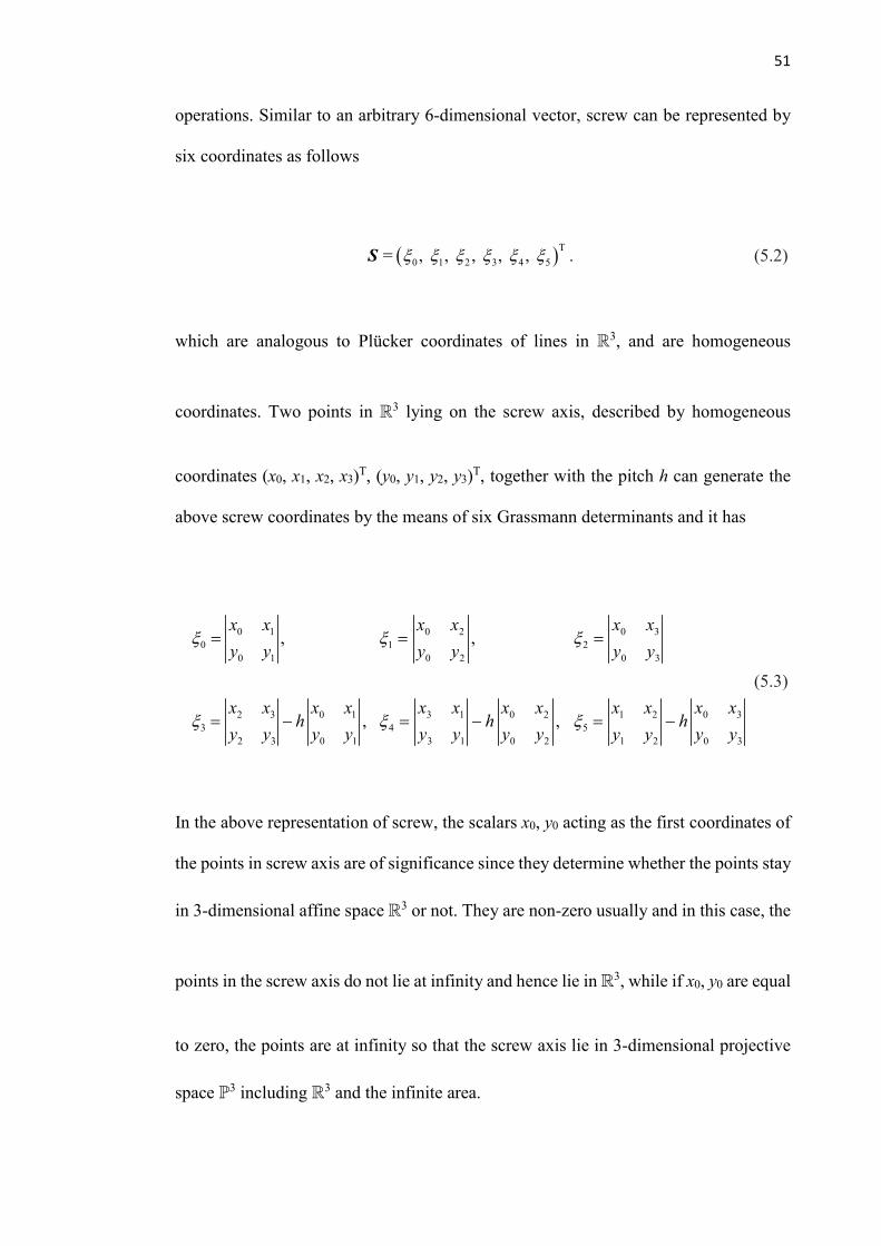
51
operations. Similar to an arbitrary 6-dimensional vector, screw can be represented by
six coordinates as follows
( )T
0 1 2 3 4 5= , , , , , S . (5.2)
which are analogous to Plücker coordinates of lines in 3, and are homogeneous
coordinates. Two points in 3 lying on the screw axis, described by homogeneous
coordinates (x0, x1, x2, x3)T, (y0, y1, y2, y3)T, together with the pitch h can generate the
above screw coordinates by the means of six Grassmann determinants and it has
0 1
0
0 1
2 3 0 1
3
2 3 0 1
,
,
x x
y y
x x x xh
y y y y
=
= -
0 2
1
0 2
3 1 0 2
4
3 1 0 2
,
,
x x
y y
x x x xh
y y y y
=
= -
0 3
2
0 3
0 31 2
5
0 31 2
x x
y y
x xx xh
y yy y
=
= -
(5.3)
In the above representation of screw, the scalars x0, y0 acting as the first coordinates of
the points in screw axis are of significance since they determine whether the points stay
in 3-dimensional affine space 3 or not. They are non-zero usually and in this case, the
points in the screw axis do not lie at infinity and hence lie in 3, while if x0, y0 are equal
to zero, the points are at infinity so that the screw axis lie in 3-dimensional projective
space 3 including 3 and the infinite area.
52
5.2.2 Screw System of nth Order
Naturally, there exists a bijective map between n-dimensional vector subspaces Vn of
six-dimensional vector space V6 spanned by n linearly independent vectors and screw
systems of order n donated as n consist precisely of all linear combinations of the
screws Si as a set of basis of n . Simultaneously, an arbitrary screw system of nth order,
also called n-system can be defined as
6
1
, , n
n i i i ii
=
= =
R VS S S S . (5.4)
At the moment screw can be seen as an element of 6-dimensional vector space V6 and
expressed by six homogenous coordinates generated by Grassmann determinates
together with pitch h as Eq. (5.3). Screw system of nth order n can be viewed as n-
dimensional vector subspace of V6.
5.3 The Helicoidal Velocity Field
Motion of a rigid body in three dimensions can be represented by a rotation about an
axis together with a translation parallel to that axis. Such motion is similar to that which
would occur if the body is connected to its surroundings by a screw thread. This general
motion is referred to as a twist on a screw axis or simply twist. A twist is a screw with
the rate amplitude and an element of the Lie algebra se(3) that can be expressed in Eq.
(5.6),

53
0 00h h
= = = ´ ´ +
sT S =
r s + s r v
. (5.5)
where S is the screw associated with the twist T, s is the direction vector of this screw,
r0 is the position vector that locates the axis of this screw, and h is the pitch gives the
ratio of the magnitude of the second component of the secondary part over that of the
primary part. The axis of rotation is the screw axis and the pitch of the screw is equal
to the ratio of the translational velocity to the rotational velocity while translation is
parallel to the axis of rotation.
With the screw axis, the body has an angular velocity . Point P on the body has
velocity vp. The velocity of any point on the body consists of a component h parallel
to the screw axis and another component normal to it expressed as ´(rp-ro) in Fig. 5.1.
Figure 5.1 Instantaneous screw axis and the helicoidal velocity field
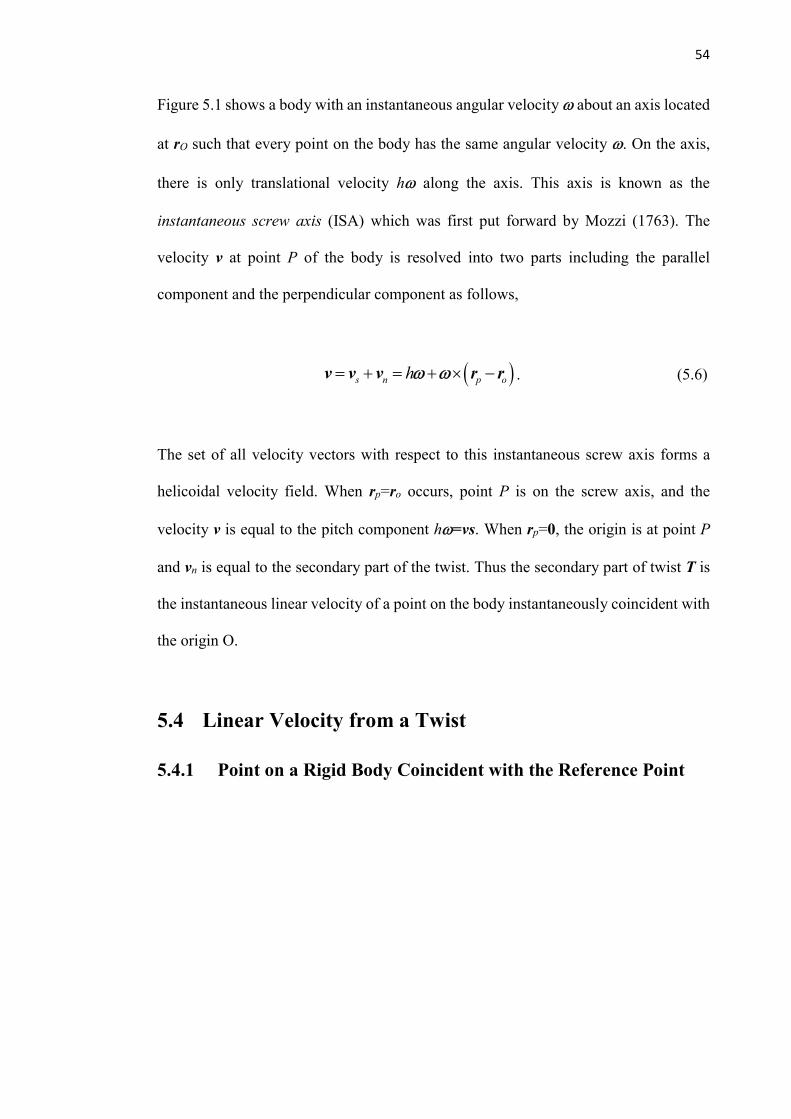
54
Figure 5.1 shows a body with an instantaneous angular velocity about an axis located
at rO such that every point on the body has the same angular velocity . On the axis,
there is only translational velocity h along the axis. This axis is known as the
instantaneous screw axis (ISA) which was first put forward by Mozzi (1763). The
velocity v at point P of the body is resolved into two parts including the parallel
component and the perpendicular component as follows,
( )s n p oh= + = + ´ -v v v r r . (5.6)
The set of all velocity vectors with respect to this instantaneous screw axis forms a
helicoidal velocity field. When rp=ro occurs, point P is on the screw axis, and the
velocity v is equal to the pitch component h=vs. When rp=0, the origin is at point P
and vn is equal to the secondary part of the twist. Thus the secondary part of twist T is
the instantaneous linear velocity of a point on the body instantaneously coincident with
the origin O.
5.4 Linear Velocity from a Twist
5.4.1 Point on a Rigid Body Coincident with the Reference Point

55
Figure 5.2 A Twist modeled by a revolute joint of a rigid body
Figure 5.2 depicts a rigid body rotates about a revolute joint with an instantaneous
angular velocity ω, which is perpendicular to the xy-plane. Without loss of generality,
we establish the reference coordinate frame in an arbitrary point O with the x-axis and
y-axis locating in the plane and z-axis directing outward the plane. The corresponding
twist of this rigid body can be expressed as,
0 0 0
= = = ´ ´
sT S =
r s r v
. (5.7)
where ||ω|| is the magnitude of the angular velocity of the rigid body, S is the joint screw
associated with the revolute joint and r0 is the position vector that directs from the origin
to the rotational axis to locate the screw axis s, v0 = r0×ω represents the instantaneous
velocity of a point on this rigid body coincident with the origin O in the xy plane. The
primary part ω, standing for the angular velocity, and the second part v0, standing for
the linear velocity constitute the twist T to describe the instantaneous motion of a rigid
body. It’s not hard to recognize that the twist of a rigid body depends on the selection
of the reference frame. If the origin of the reference frame concurs with the revolute

56
joint; that is r0 = 0, the linear velocity vanishes and the twist represents a pure
differential rotation.
5.4.2 Geometrical Meaning of Secondary Part of a Screw
A serial manipulator is comprised of sequential rigid bodies connected with mechanical
pairs. The twists that depict the instantaneous motion of components in this manipulator
can be assembled to generate a resultant twist in such a way to describe the
instantaneous motion of the end-effector with respect to the global reference frame.
The geometrical interpretation of the resultant twist is exemplified with a planar 3R
serial mechanism, exhibited in Fig. 5.3.
Figure 5.3 Geometry representation of a resultant twist in a serial manipulator

57
Links OA, AB and BC are serially connected by revolute joints O, A and B that
constructs this 3R serial mechanism. The reference coordinate system is attached to
ground with its origin O matching with the first revolute joint O and z-axis directing
outward the plane. The time derivative of the rotation of link OA, which is noted as the
twist of link OA with respect to the ground, can be expressed as
1 1
1 1 1 1
10 1 1
= = = ´
ω sT ω ω S
v r s. (5.8)
where ω1 is the angular velocity of joint O, v10 is the linear velocity of link OA, which
indicates the velocity of the point on OA coincident with the origin, S1 is the joint screw
of joint O with s1 representing the direction vector of this joint screw. Similarly, the
twist of link AB with respect to the link OA in the coordinate frame is described as
2 2
2 2 2 2
20 2 2
= = = ´
ω sT ω ω S
v r s. (5.9)
where ω2 is the angular velocity of joint A, r2 is the position vector that determines the
position of screw axis s2 of the joint screw S2, v20 is the linear velocity of the point on
link AB coincident with the origin O instantaneously.The twist of link BC with respect
to link AB is described as
3 3
3 3 3 3
30 3 3
= = = ´
ω sT ω ω S
v r s. (5.10)
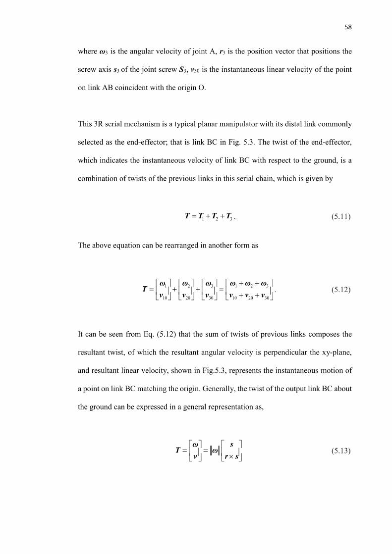
58
where ω3 is the angular velocity of joint A, r3 is the position vector that positions the
screw axis s3 of the joint screw S3, v30 is the instantaneous linear velocity of the point
on link AB coincident with the origin O.
This 3R serial mechanism is a typical planar manipulator with its distal link commonly
selected as the end-effector; that is link BC in Fig. 5.3. The twist of the end-effector,
which indicates the instantaneous velocity of link BC with respect to the ground, is a
combination of twists of the previous links in this serial chain, which is given by
1 2 3= + +T T T T . (5.11)
The above equation can be rearranged in another form as
1 2 3 1 2 3
10 20 30 10 20 30
+ + = + + = + +
ω ω ω ω ω ωT
v v v v v v. (5.12)
It can be seen from Eq. (5.12) that the sum of twists of previous links composes the
resultant twist, of which the resultant angular velocity is perpendicular the xy-plane,
and resultant linear velocity, shown in Fig.5.3, represents the instantaneous motion of
a point on link BC matching the origin. Generally, the twist of the output link BC about
the ground can be expressed in a general representation as,
= = ´
ω sT ω
v r s (5.13)
59
where s indicates the instantaneous screw axis (ISA) of the twist T, and r is the position
vector from the origin pointing to the screw axis. Combining the Eqs. (5.12) and (5.13)
yields the resultant angular velocity and resultant linear velocity of the end-effector BC
as follows
1 2 3= + +ω ω ω ω , (5.14)
10 20 30= + +v v v v . (5.15)
It can be seen from Eqs. (5.14), the resultant angular velocity which composes the twist
of the effector in a serial robot is the sum of the angular velocities of previous links.
The direction of the angular velocity follows the ISA of the resultant twist. In addition,
the linear velocity which composes the secondary part of the resultant twist is the sum
of the linear velocities of previous links, and its direction is compounded by the each
individual elements.
5.4.3 Position Vector of the Resultant Twist
It is illustrated that the angular velocity ω1, ω2 and ω3 have the same direction in Fig.
5.3 that points outward the plane, so the magnitude of resultant angular velocity ω is
1 2 3= + +ω ω ω ω . (5.16)
Substituting linear velocities of the Eqs. (5.8) to (5.10) into Eq. (5.16) yields
( ) ( ) ( ) ( )1 1 1 2 2 2 3 3 3´ = ´ + ´ + ´ω r s ω r s ω r s ω r s . (5.17)
60
Since s1, s2 and s3 have the same direction with s, the above equation can be written in
a compact form as
( ) ( )1 1 2 2 3 3´ = + + ´ω r s ω r ω r ω r s . (5.18)
The direction vector si of the joint screw Si (i=1,2,3) align with the z-axis, which has
the relation s1=s2=s3=s, the position vector of the resultant twist that situates the ISA is
the linear combination of weighted position vectors of all the joints, which is expressed
as
1 2 3
1 2 3= + +ω ω ω
r r r rω ω ω
. (5.19)
The position vectors of all the joint screws and corresponding joint rates comprise the
position vector that determines the location of the ISA associated with the resultant
twist of the end-effector.
5.4.4 Coordinated ISA of the End-Effector of a Serial Manipulator
As mentioned, the instantaneous motion of a rigid body composes of a differential
rotation about a unique axis and the differential translation along this axis. This axis is
named as the instantaneous screw axis of this differential motion. Suppose an arbitrary
point Q is located at the ISA, it can thus be seen that the linear velocity of point Q is
equal to translational velocity along this ISA. The twist of Q is given by
61
0 0
q q
q q q qh
= = ´ +
ω ωT
v r ω ω. (5.20)
where ωq, vq0, and h represent the angular velocity, linear velocity and pitch of this
instantaneous motion on point Q, respectively, and rq0 is perpendicular to the angular
velocity vector ωq. To obtain the position vector rq0, we take the cross product of ωq
and vq0, that yields
( ) ( ) ( ) 20 0 0 0 0q q q q q q q q q q q q q´ = ´ ´ = - =ω v ω r ω r ω ω ω ω r ω r . (5.21)
Dividing both sides of the Eq. (5.21) by ωq2 yields,
0
0 2
q q
q
q
´=
ω vr
ω. (5.22)
Equation (5.22) shows that the position vector of point Q is calculated by the inverse
square of the angular velocity times cross product of the angular velocity and
instantaneous linear velocity of point Q. As Q is an arbitrary point on the ISA, its
position can be expressed as,
0
0 2
q q
q q q q
q
´
+ = +ω v
r = r ω ωω
(5.23)
where λ is an arbitrary scalar.
The ISA of the end-effector in a serial manipulator can be obtained from Eq. (5.23) by
replacing the angular velocity and linear velocity with the resultant angular velocity and
62
velocity of the end-effector, whose points on the axis only have the angular velocity
and the linear velocity vanishes.
5.5 Screw based Jacobian Derivation of Serial Robots
5.5.1 Jacobian Matrix of a Planar Serial Manipulator
As a fundamental topic in robotics, kinematics play a crucial role in identifying the
functionality and performance of a robot. The mathematical relation that maps the joint
displacements to the position and orientation of the end-effector of a manipulator forms
the forward kinematics analysis, whereas the inverse kinematics relates the end-effector
configuration to joint movements. The first-order kinematics analysis gives the velocity
map that establishes the relationship between joint rates and velocity state of the end-
effector, which is also known as Jacobian matrix or Jacobian. Screw algebra has the
capability to formulate the Jacobian to bridge the velocity map from joint space to task
space of a manipulator.
Figure 5.4 displays a planar 3R serial robot with the distal link as the end-effector. The
reference coordinate {O-xyz} is established at the origin O with the x-axis aligns the
horizontal line and z-axis directs outward the plane. The three links OA, AB, and BC
are serially connected through revolute pair with the joint axis perpendicular to the
plane. The displacement of joint O, which represents the relative rotation of link OA
with respect to the x-axis of the coordinate systems, is denoted as θ1. Similar to this
definition, the displacements of joint B and joint C are described as θ2 and θ3,
respectively.

63
We derive the screw algebra based Jacobian of the 3R planar serial manipulator. In the
reference coordinate frame {O-xyz}, the axes of the revolute joints O, A, B have the
same direction with z-axis as s1 = s2 = s3 = [0, 0, 1]T. The position vectors that locate
the joint A and B can be derived from the geometry of the manipulator as rA = [l1cθ1,
l1sθ1, 0]T, and rB = [l1cθ1+ l2cθ12, l1cθ1+ l2cθ12, 0]T, where s and c stand for the sine and
cosine functions, and θ12 stands θ1+θ2.
Figure 5.4 A 3R planar serial manipulator
The normalized motion screws of the revolute joints O, A, and B are given by in the
reference frame as,
T
1 0, 0,1, 0, 0, 0
= = 0
zS (5.24)
T
2 1 1 1 1
2
0 0 1 s c 0l l
= = - ´
zS
r z (5.25)
T3 1 1 2 12 1 1 2 12
3
0 0 1 s c 0l l s l l c
= = + - - ´
zS
r z (5.26)
64
The twist of the link BC with respect to the ground is expressed by substituting Eqs.
(5.24) to (5.26) into Eq. (5.11) as follows,
1
1 1 2 2 3 3 1 2 3 2
3
BC
BC
= + + = =
=ω
T S S S S S S Jθv
(5.27)
where the joint velocity vector T
1 2 3 = θ and Jacobin is
1 1 1 1 2 12
1 1 1 1 2 12
0 0 0
0 0 0
1 1 1
0 s
0
0 0 0
l s l l s
l c l c l cs
= +
- - -
J (5.28)
The columns of the Jacobian are the unit joint screws of this manipulator, while their
corresponding magnitudes comprise the joint velocity vector. It can be seen from the
Eq. (5.27) that the screw theory based Jacobian is irrelevant with the distal joint variable.
5.5.2 Resultant Twist of a Spatial Serial Manipulator
It can be seen from the Eq. (5.11) the twist of the end-effector in a 3R serial manipulator
is the sum of the twists of previous links. To be more general, the twist of a serial robot
is the assemblage of twists of previous links as,
1 1
n n
i i ii i
q= =
= =
ωT = T S
v (5.29)
65
where ω is the angular velocity of the end-effector, while v is the linear velocity
coincident with the origin of the reference coordinate frame, iq is the rate of change of
each joint, and Si is the unit screw associated with the joint axis in this manipulator.
The Jacobian can be obtained if all the joint screws of a serial manipulator are identified
in one coordinate frame. It turns out that the coordinates of the joint screws can be
written in any reference frames by investigating the geometry of the manipulator. As
the joint axis and its position determine the corresponding joint screw for typical serial
manipulators composed of prismatic joints or revolute joints, the Jacobian is
accomplished through the geometry of the manipulator.
5.6 Conclusions
This chapter investigated the motion of a rigid body in three dimensions that could be
decomposed into a rotation about an axis and a translation parallel to that axis. The
motion could be represented by a twist with its primary part indicating the angular
velocity of the rigid body, and secondary part indicating the instantaneous linear
velocity.
The resultant twist of a serial manipulator could be presented by the assembly of unit
joint screws with their corresponding velocity amplitudes. The ISA of the resultant twist
was coordinated through the condition of zero linear velocity on this axis, and its
position vector was formulated by the combination of weighted position vectors of joint
screws. The screw-based Jacobian of a planar serial manipulator was established after
identifying all the joint screws, followed by the expansion to general serial manipulators.
66
Chapter 6 Geometrical Interpretation of the
Transformation between Robot Jacobian and
Screw Jacobian
6.1 Introduction
This chapter investigates the relationship of the Jacobians of a serial manipulator with
the derivative method and screw theory. Forward kinematics analysis of a typical 3R
planner manipulator is formulated, followed by its time derivative to generate the
conventional Jacobian. Its counterpart, the screw-based Jacobian is developed with the
assemblage of all the unit joint screws. The comparison from both geometrical meaning
and physical meaning is conducted in an attempt to accomplish the reconciliation of the
two methods. Further, a more complicated spatial kinematic chain is investigated to
verify the derivation.
The transformation between conventional Jacobian and screw Jacobian is revealed
through investigating the geometry meaning of the resultant twist of the end-effector
and the velocity of a reference point. The Jacobian matrices are formulated by the
derivative method and screw algebra and their relation is interpreted.
67
6.2 Derivative Method based Jacobian of a 3R Planar
Serial Manipulator
6.2.1 Linear Velocity of a 3R Planar Serial Manipulator
The position and orientation of a serial manipulator can be obtained in the wake of
forward kinematics analysis. The Jacobian matrix that describes the motion of a rigid
body in the velocity field is conventionally derived through the differential kinematics.
The forward kinematics of a serial manipulator can be developed in various methods
such as Denavit-Hartenberg matrices [102], screw algebra, etc. A typical planar
manipulator is shown in Fig. 5.4. To acquire the translational velocity of point C, a
geometric method is to find its position and then take its time derivative. The position
of point C in the reference coordinate frame {O-xyz} can be derived from the geometry
of the 3R manipulator as,
C 1 1 2 12 3 123
C 1 1 2 12 3 123
C
c c c
s s s
0C
x l l l
P y l l l
z
+ + = = + +
(6.1)
where θijk is the simplified representation of θi+ θj+ θk. Taking the time derivation of
the position of point C with respect to the global frame gives its linear velocity vC,
which can be expressed as,
1 1 1 12 2 12 123 3 123
1 1 1 12 2 12 123 3 123
0
C
C C
C
x l s l s l s
y l c l c l c
z
- - - = = + +
v
(6.2)
68
where 123 stands for 1 2 3 + + . Different from the linear velocity derived from screw
algebra which indicates the instantaneous velocity of the point on a rigid body
coincident with the origin, the linear velocity vC represents the velocity of point C with
respect to the origin. The two types of velocities can both describe the instantaneous
state of the end-effector of a serial manipulator, and are usually not identical. The
relation of these velocities will be discussed in the following sections.
6.2.2 Jacobian Generation based on the Derivative Method
Shown in Eq. (6.2), the linear velocity of point C is determined by the angular velocity
of all the joints connected from the ground and current configuration of the manipulator.
From the geometry of the manipulator, the orientation of link BC is the sum of joint
displacement of joint O, A and B, which is expressed as,
1 2 3C = + + (6.3)
Taking the time derivative of Eq. (6.3) yields the angular velocity of point C, which is
written in a vector form as,
1 2 3
0
0C
= + +
ω
(6.4)
Combining the Eqs. (6.2) and (6.4) and rearranging the vectors yields the velocity of
point C expressed in the reference frame as,
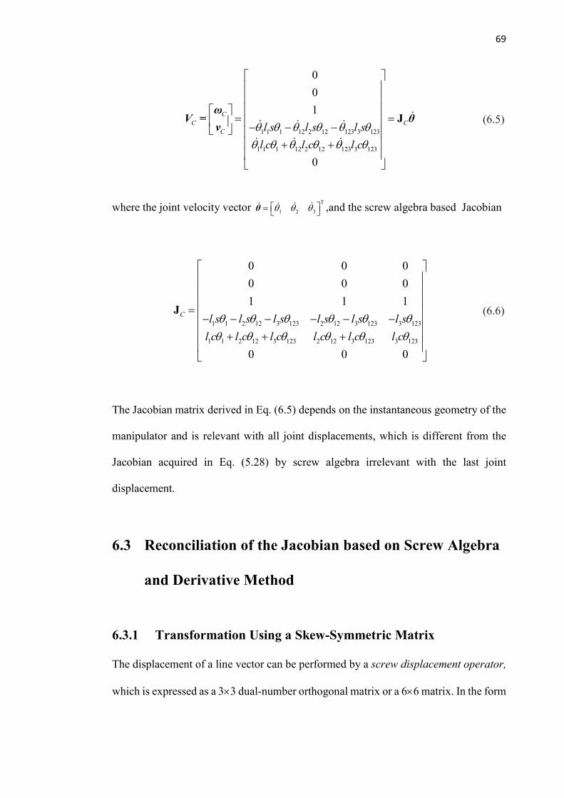
69
1 1 1 12 2 12 123 3 123
1 1 1 12 2 12 123 3 123
0
0
1
0
C
C C
C l s l s l s
l c l c l c
= = - - - + +
= Jω
V θv
(6.5)
where the joint velocity vector T
1 2 3 = θ ,and the screw algebra based Jacobian
1 1 2 12 3 123 2 12 3 123 3 123
1 1 2 12 3 123 2 12 3 123 3 123
0 0 0
0 0 0
1 1 1
0 0 0
Cl s l s l s l s l s l s
l c l c l c l c l c l c
= - - - - - - + + +
J (6.6)
The Jacobian matrix derived in Eq. (6.5) depends on the instantaneous geometry of the
manipulator and is relevant with all joint displacements, which is different from the
Jacobian acquired in Eq. (5.28) by screw algebra irrelevant with the last joint
displacement.
6.3 Reconciliation of the Jacobian based on Screw Algebra
and Derivative Method
6.3.1 Transformation Using a Skew-Symmetric Matrix
The displacement of a line vector can be performed by a screw displacement operator,
which is expressed as a 3´3 dual-number orthogonal matrix or a 6´6 matrix. In the form
70
of the 3´3 dual-number matrix, a displacement acting on a line vector is given by the
following operator
+R AR , (6.7)
where matrix R is a 3×3 rotation matrix that belongs to the special orthogonal group
SO(3) as the primary part of the dual-number matrix, matrix A is a skew-symmetric
matrix representing the translation in the form of,
0
0
0
z y
z x
y x
d d
d d
d d
-
- = ´ -
A = d (6.8)
This matrix leads to a translation of the rotated line vector with a distance d. Besides
this representation, the dual-number matrix can be expressed in the form of a 6×6 finite
displacement-screw matrix as
=
R 0T
A R R, (6.9)
Where matrices R and AR are the primary part and second part, respectively. Acting
the 6×6 displacement matrix in Eq. (6.9) on a line vector results in the corresponding
displacement of this line vector. Further, exerting this 6×6 finite displacement-screw
matrix on a screw, the new screw after the displacement is given by,
00 0
' = = = = ´ ++
RRR 0T
R RAR RAR R
ss sS S
d s ss s s (6.10)
71
6.3.2 Reconciliation of the Jacobian of a 3R Serial Manipulator
The physical meaning of the linear velocity vC exhibited in Eq. (6.2) is the linear
velocity of point C with respect to the origin expressed in the reference coordinate frame.
Dissimilarly, the physical meaning of the twist of link BC exhibited in Eq. (5.27)
comprise the angular velocity and linear velocity of link BC, of which the linear
velocity vC0 represents the instantaneous linear velocity of a point on the link BC
instantaneously coincident with the origin O. Based on this definition, we can draw the
conclusion that vC0 and vC are the linear velocities of link BC expressed in different
reference points, namely point C and the point instantaneously coincident with the
origin O, respectively. As the one rigid body has the same angular velocity everywhere,
we adopt ω = ωC = ωBC for simplified notation. This mentioned interrelation leads to
translating vC0 from the origin to point C to acquire vC, which is given by,
C OB BC= ´ +v ω r v (6.11)
The Eq. (6.11) is demonstrated in Appendix A. Rewriting the Eq. (6.11) with angular
velocities in a matrix form as,
C BC
BC OB BC BCO
= = - ´´ +
I
r I
0ω ω ω
v ω r v v (6.12)
Substituting Eqs. (5.27) and (6.5) into Eq.(6.12) to obtain the relationship of Jacobian
matrices derived by the derivative method and screw algebra which is given by,

72
C C
BO
= - ´
I
r I
0V = J θ Jθ (6.13)
The Jacobian acquired from derivative method and the Jacobian acquired from screw
algebra have the following relation as,
( )B B
= =AdD S S SO O
g
= - ´ ´ J J
r r
I 0 I 0J J
I I (6.14)
where g has the effect of translation from point B to origin O.
More generally, the relationship between the twist of a rigid body and the velocity of
point P on this rigid body can be established by substituting the secondary part of
Eq.(5.5) into Eq. (5.6), which yields,
o p o ph= ´ + ´ = + ´v r r v r- (6.15)
Equation (6.15) can be written in a similar matrix form with Eq. (5.15) as,
o p p o p
= = = + ´ - ´ - ´
I 0 I 0
I IT
v r r v rv
(6.16)
Equations (6.13) and (6.16) illustrates the interrelation of velocities of a rigid body with
different reference points, typically a point attached to the end-effector and the point
instantaneous coincident with the origin. The velocity of a point in the end-effector, or
the origin of the tool frame of the serial manipulator, can be generated by the
differentiation of its position and orientation calculated by transformation matrices with

73
DH parameters. The screw algebra is another method to acquire velocity of the point
on the output link instantaneous matching the origin of the reference frame.
Reconciliation of the two velocities is built by the velocity translation formulated in Eq.
(6.12), followed by the reconciliation of Jacobian matrices obtained from the derivative
method and screw algebra formulated in Eq. (6.13)
6.4 Reconciliation of Jacobian Matrices a Spatial Serial
Manipulator
6.4.1 Screw Algebra based Jacobian for a Spatial Serial
Manipulator
The transformation between screw based Jacobian and derivative method based
Jacobian was proposed, followed by the verification of a planar serial Manipulator. In
this section, a more complicated example was used to formulate the Jacobian matrices.
Figure 6.1 shows a RRPRR spatial serial manipulator. The global coordinate frame {O0-
x0y0z0} is fixed at point O0, its z0-axis aligns along the axis of the first revolute joint,
and ix0-axis lies along the axis of the second revolute joint in its initial configuration.
The motion screw Si (i = 1 to 5) are attached to each joint shown in Fig. 6.1.
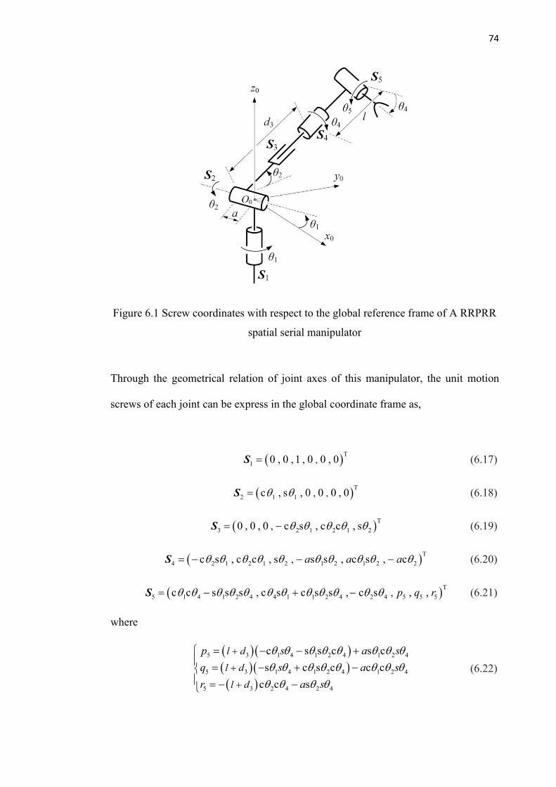
74
Figure 6.1 Screw coordinates with respect to the global reference frame of A RRPRR
spatial serial manipulator
Through the geometrical relation of joint axes of this manipulator, the unit motion
screws of each joint can be express in the global coordinate frame as,
( )T
1 ,,0 , 0 , 1 0 0 , 0=S (6.17)
( )T
2 1 1 ,,c , s , 0 0 0 , 0 =S (6.18)
( )T
3 2 1 2 1 2,0 , 0 , 0 c s , c c , s = -S (6.19)
( )T
4 2 1 2 1 2 1 2 1 2 2,c s , c c , s s s , c s , ca a a = - - -S (6.20)
( )T
5 1 4 1 2 4 4 1 1 2 4 2 4 5 5 5,c c s s s , c s c s s , c s , ,p q r = - + -S (6.21)
where
( ) ( )( ) ( )( )
5 3 1 4 1 2 4 1 2 4
5 3 1 4 1 2 4 1 2 4
5 3 2 4 2 4
c s s c s c
s c s c c c
c c s
l d
l d
l d
p s a s
q s a s
r a s
+
+
+
= - - +
= - + - = - -
(6.22)
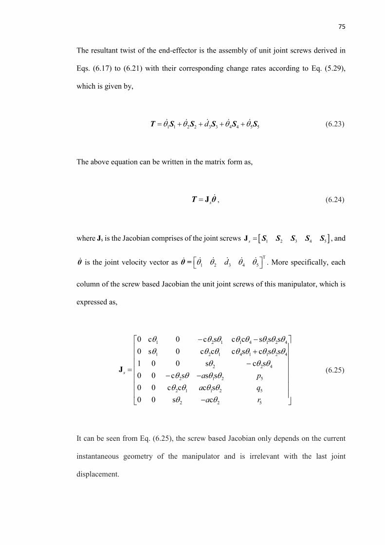
75
The resultant twist of the end-effector is the assembly of unit joint screws derived in
Eqs. (6.17) to (6.21) with their corresponding change rates according to Eq. (5.29),
which is given by,
1 1 2 2 3 3 4 4 5 5d = + + + +T S S S S S (6.23)
The above equation can be written in the matrix form as,
s= JT θ , (6.24)
where Js is the Jacobian comprises of the joint screws 1 2 3 4 5s =J S S S S S , and
θ is the joint velocity vector as T
1 2 3 4 5d θ = . More specifically, each
column of the screw based Jacobian the unit joint screws of this manipulator, which is
expressed as,
1 2 1 1 4 1 2 4
1 2 1 4 1 1 2 4
2 2 4
2 1 2 5
2 1 1 2 5
2 2 5
0 c 0 c s c c s s s
0 s 0 c c c s c s s
1 0 0 s c s
0 0 c s s s
0 0 c c c s
0 0 s c
s a p
a q
a r
- - +
- =
- -
-
J (6.25)
It can be seen from Eq. (6.25), the screw based Jacobian only depends on the current
instantaneous geometry of the manipulator and is irrelevant with the last joint
displacement.
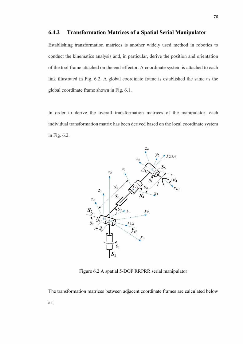
76
6.4.2 Transformation Matrices of a Spatial Serial Manipulator
Establishing transformation matrices is another widely used method in robotics to
conduct the kinematics analysis and, in particular, derive the position and orientation
of the tool frame attached on the end-effector. A coordinate system is attached to each
link illustrated in Fig. 6.2. A global coordinate frame is established the same as the
global coordinate frame shown in Fig. 6.1.
In order to derive the overall transformation matrices of the manipulator, each
individual transformation matrix has been derived based on the local coordinate system
in Fig. 6.2.
Figure 6.2 A spatial 5-DOF RRPRR serial manipulator
The transformation matrices between adjacent coordinate frames are calculated below
as,
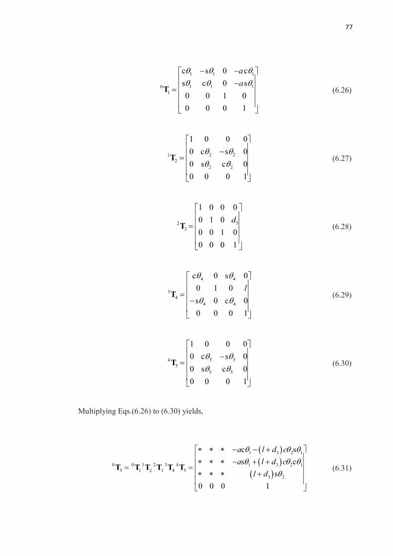
77
1 1 1
1 1 101
c s 0 c
s c 0 s
0 0 1 0
0 0 0 1
a
a
- - - =
T (6.26)
2 21
2
2 2
1 0 0 0
0 c s 0
0 s c 0
0 0 0 1
- =
T (6.27)
32
3
1 0 0 0
0 1 0
0 0 1 0
0 0 0 1
d
=
T (6.28)
4 4
34
4 4
c 0 s 0
0 1 0
s 0 c 0
0 0 0 1
l
=-
T (6.29)
5 54
5
5 5
1 0 0 0
0 c s 0
0 s c 0
0 0 0 1
- =
T (6.30)
Multiplying Eqs.(6.26) to (6.30) yields,
( )( )
( )
1 3 2 1
0 0 1 2 3 4 1 3 2 15 1 2 3 4 5
3 2
c s
s c
s
0 0 0 1
a l d c
a l d c
l d
- - + - + + = = +
T T T T T T (6.31)
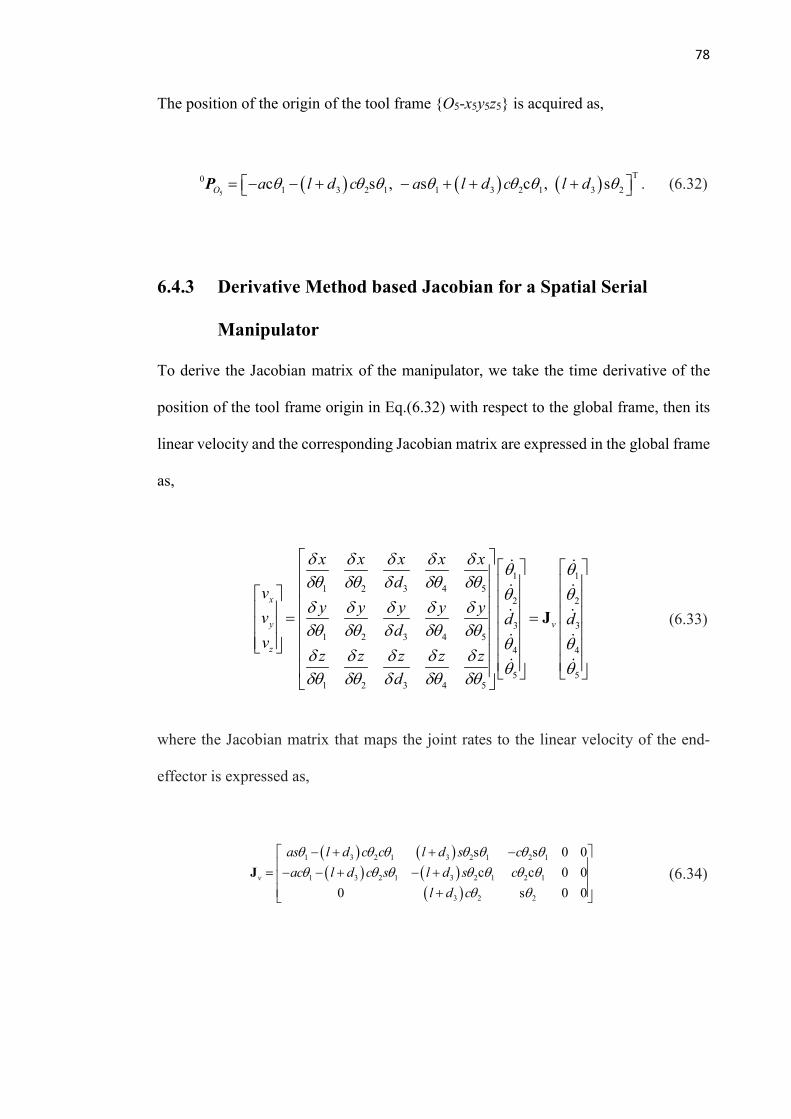
78
The position of the origin of the tool frame {O5-x5y5z5} is acquired as,
( ) ( ) ( )5
T01 3 2 1 1 3 2 1 3 2c s , s c , sO a l d c a l d c l d = - - + - + + + P . (6.32)
6.4.3 Derivative Method based Jacobian for a Spatial Serial
Manipulator
To derive the Jacobian matrix of the manipulator, we take the time derivative of the
position of the tool frame origin in Eq.(6.32) with respect to the global frame, then its
linear velocity and the corresponding Jacobian matrix are expressed in the global frame
as,
1 1
1 2 3 4 5
2 2
3 31 2 3 4 5
4 4
5 51 2 3 4 5
x
y v
z
x x x x x
dv
y y y y yv d d
dv
z z z z z
d
= =
J
(6.33)
where the Jacobian matrix that maps the joint rates to the linear velocity of the end-
effector is expressed as,
( ) ( )( ) ( )
( )
1 3 2 1 3 2 1 2 1
1 3 2 1 3 2 1 2 1
3 2 2
s s 0 0
c c 0 0
0 s 0 0v
as l d c c l d s c
ac l d c s l d s c
l d c
- + + -
= - - + - + +
J (6.34)
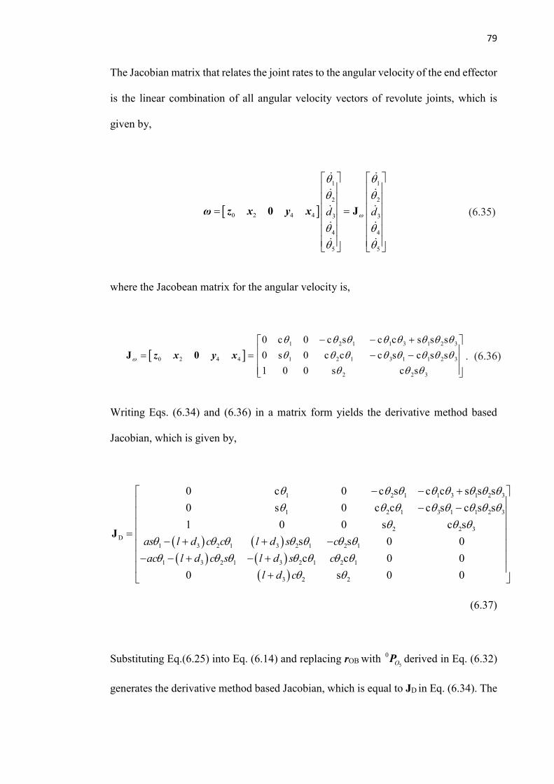
79
The Jacobian matrix that relates the joint rates to the angular velocity of the end effector
is the linear combination of all angular velocity vectors of revolute joints, which is
given by,
1 1
2 2
0 2 4 4 3 3
4 4
5 5
d d
= =
0 Jω z x y x
(6.35)
where the Jacobean matrix for the angular velocity is,
1 2 1 1 3 1 2 3
0 2 4 4 1 2 1 3 1 1 2 3
2 2 3
0 c 0 c s c c s s s
0 s 0 c c c s c s s
1 0 0 s c s
- - + = = - -
J 0z x y x . (6.36)
Writing Eqs. (6.34) and (6.36) in a matrix form yields the derivative method based
Jacobian, which is given by,
( ) ( )( ) ( )
( )
1 2 1 1 3 1 2 3
1 2 1 3 1 1 2 3
2 2 3
D1 3 2 1 3 2 1 2 1
1 3 2 1 3 2 1 2 1
3 2 2
0 c 0 c s c c s s s
0 s 0 c c c s c s s
1 0 0 s c s
s s 0 0
c c 0 0
0 s 0 0
as l d c c l d s c
ac l d c s l d s c
l d c
- - + - -
= - + + -
- - + - +
+
J
(6.37)
Substituting Eq.(6.25) into Eq. (6.14) and replacing rOB with 5
0OP derived in Eq. (6.32)
generates the derivative method based Jacobian, which is equal to JD in Eq. (6.34). The
80
transformation of the screw based Jacobian and derivative method based Jacobian is
verified.
6.5 Conclusions
This chapter revealed the interrelation of the screw-based Jacobian and derivative
method-based Jacobian through investigating the geometrical meaning of a twist of a
rigid body and the velocity of a reference point on this rigid body. Reconciliation of
these two methods was formulated by using an adjoint transformation acting on a twist
obtained by screw algebra.
Exampled by a planar 3R serial manipulator, the reconciliation was coordinated and
interrelation was exposed. Further, velocity analysis of a more complicated spatial
serial manipulator was studied by screw algebra and Denvit-Hartenberg method with
the interrelation of Jacobian matrices verified.
81
Chapter 7 Screw Jacobian Analysis of a
Reconfigurable Platform-Based Parallel
Mechanism
7.1 Introduction
Parallel mechanisms, in general, have a rigid base and a moving platform connected by
several limbs. For achieving higher mobility and dexterity, more degrees of freedom
are introduced to the limbs. However, very few researchers focus on changing the
design of the rigid base and making it foldable and reconfigurable to improve the
performance of the mechanism.
Inspired by manipulating an object with a metamorphic robotic hand, this chapter
presents a parallel mechanism with a reconfigurable base. This novel spherical-base
integrated parallel mechanism has an enlarged workspace compared with traditional
parallel manipulators. Evolution and structure of the proposed parallel mechanism is
introduced and the geometric constraint of the mechanism is investigated based on
mechanism decomposition. Further, kinematics of the proposed mechanism is reduced
to the solution of a univariate polynomial of degree 8. Moreover, screw theory based
Jacobian[64] is presented followed by the velocity analysis of the mechanism.

82
7.2 A Spherical-Base Integrated Parallel Mechanism
7.2.1 From Manipulation with a Metamorphic Hand to a Parallel
Mechanism with a Reconfigurable Base
Figure 7.1 illustrates a three-fingered metamorphic robotic hand grasping and
manipulating a disk. The metamorphic robotic hand contains a reconfigurable palm and
three two-phalanx fingers. The reconfigurable palm is formed by a spherical five-bar
linkage, with link AE as a grounded link, and the other four links are symmetrically
arranged with respect to link AE such that links AB and ED are of the same length and
so do links BC and DC. The three fingers are respectively mounted on link AE at point
A1, on link DC at point A2 and on link BC at point A3. When the palm is in a
configuration that all the links are in the same plane, the three points A1, A2 and A3 are
evenly distributed about point O, i.e. centre of the spherical five-bar linkage. The 2-
DOF reconfigurable palm changes configuration of the whole hand, and increases
workspace, dexterity and manipulability of the hand[60,61]. The idea of equivalence
about considering the multi-fingered hand with a grasped object as a parallel
mechanism was put forward by Borras-Sol and Dollar[62,63]. When the hand is used
to grasp and manipulate an object such as a disk as shown in Fig. 1, if the contact points
between the object and the fingertips are thought of as spherical joints, an equivalent
parallel mechanism with a reconfigurable base can be intuitively generated as illustrated
in Fig. 2. This parallel mechanism is coined in this chapter spherical-base integrated
parallel mechanism.
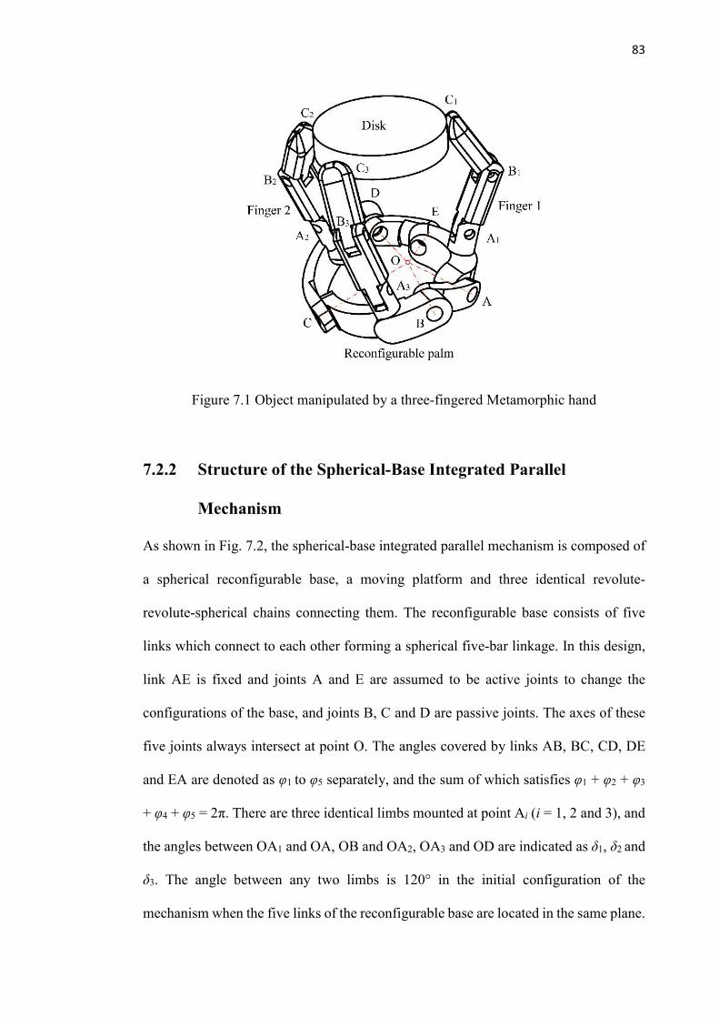
83
Figure 7.1 Object manipulated by a three-fingered Metamorphic hand
7.2.2 Structure of the Spherical-Base Integrated Parallel
Mechanism
As shown in Fig. 7.2, the spherical-base integrated parallel mechanism is composed of
a spherical reconfigurable base, a moving platform and three identical revolute-
revolute-spherical chains connecting them. The reconfigurable base consists of five
links which connect to each other forming a spherical five-bar linkage. In this design,
link AE is fixed and joints A and E are assumed to be active joints to change the
configurations of the base, and joints B, C and D are passive joints. The axes of these
five joints always intersect at point O. The angles covered by links AB, BC, CD, DE
and EA are denoted as φ1 to φ5 separately, and the sum of which satisfies φ1 + φ2 + φ3
+ φ4 + φ5 = 2π. There are three identical limbs mounted at point Ai (i = 1, 2 and 3), and
the angles between OA1 and OA, OB and OA2, OA3 and OD are indicated as δ1, δ2 and
δ3. The angle between any two limbs is 120° in the initial configuration of the
mechanism when the five links of the reconfigurable base are located in the same plane.
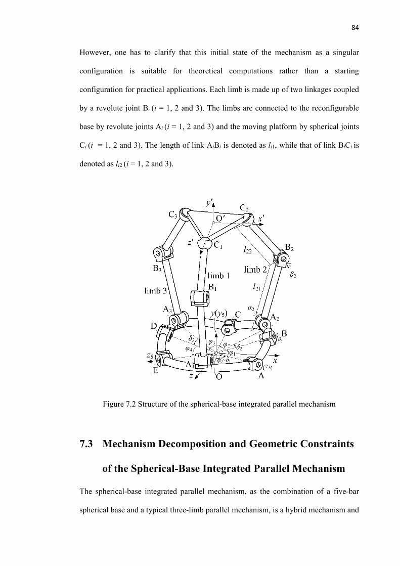
84
However, one has to clarify that this initial state of the mechanism as a singular
configuration is suitable for theoretical computations rather than a starting
configuration for practical applications. Each limb is made up of two linkages coupled
by a revolute joint Bi (i = 1, 2 and 3). The limbs are connected to the reconfigurable
base by revolute joints Ai (i = 1, 2 and 3) and the moving platform by spherical joints
Ci (i = 1, 2 and 3). The length of link AiBi is denoted as li1, while that of link BiCi is
denoted as li2 (i = 1, 2 and 3).
Figure 7.2 Structure of the spherical-base integrated parallel mechanism
7.3 Mechanism Decomposition and Geometric Constraints
of the Spherical-Base Integrated Parallel Mechanism
The spherical-base integrated parallel mechanism, as the combination of a five-bar
spherical base and a typical three-limb parallel mechanism, is a hybrid mechanism and
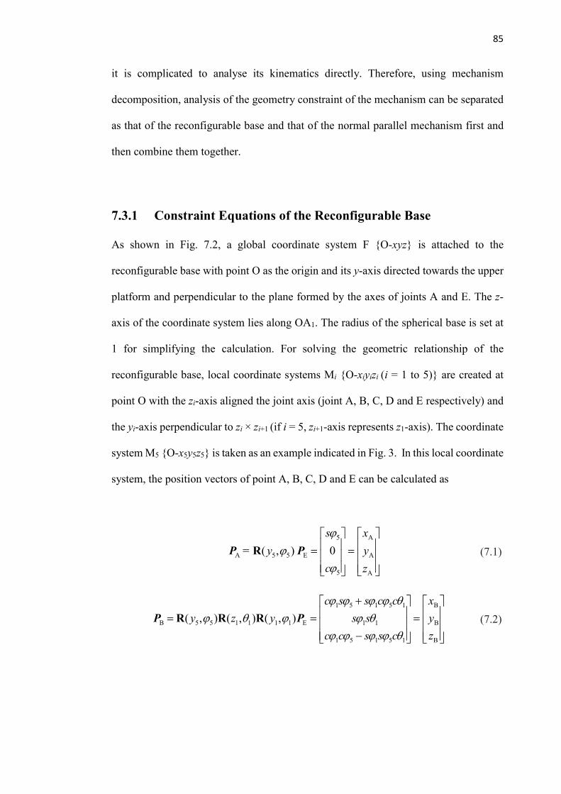
85
it is complicated to analyse its kinematics directly. Therefore, using mechanism
decomposition, analysis of the geometry constraint of the mechanism can be separated
as that of the reconfigurable base and that of the normal parallel mechanism first and
then combine them together.
7.3.1 Constraint Equations of the Reconfigurable Base
As shown in Fig. 7.2, a global coordinate system F {O-xyz} is attached to the
reconfigurable base with point O as the origin and its y-axis directed towards the upper
platform and perpendicular to the plane formed by the axes of joints A and E. The z-
axis of the coordinate system lies along OA1. The radius of the spherical base is set at
1 for simplifying the calculation. For solving the geometric relationship of the
reconfigurable base, local coordinate systems Mi {O-xiyizi (i = 1 to 5)} are created at
point O with the zi-axis aligned the joint axis (joint A, B, C, D and E respectively) and
the yi-axis perpendicular to zi × zi+1 (if i = 5, zi+1-axis represents z1-axis). The coordinate
system M5 {O-x5y5z5} is taken as an example indicated in Fig. 3. In this local coordinate
system, the position vectors of point A, B, C, D and E can be calculated as
5 A
A 5 5 E A
5 A
( , ) 0
s x
= y y
c z
= =
RP P (7.1)
1 5 1 5 1 B
B 5 5 1 1 1 1 E 1 1 B
1 5 1 5 1 B
( , ) ( , ) ( , )
c s s c c x
y z y s s y
c c s s c z
+ = = =
-
R R RP P (7.2)
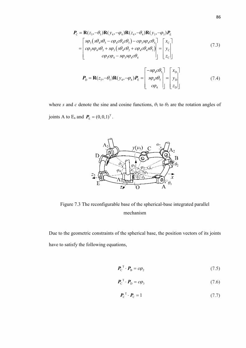
86
( )
( )
C 5 5 4 4 4 4 3 3 E
3 4 5 4 4 5 3 4 5 C
3 4 5 3 4 5 4 4 5 C
3 4 3 4 4 C
( , ) ( , ) ( , ) ( , )z y z y
s s s c c c c s c x
c s s s s c c c s y
c c s s c z
= - - - -
- - = + + = -
R R R RP P
(7.3)
4 5 D
D 5 5 4 4 E 4 5 D
4 D
( , ) ( , )
s c x
z y s s y
c z
- = - - = =
R RP P (7.4)
where s and c denote the sine and cosine functions, θ1 to θ5 are the rotation angles of
joints A to E, and TE (0,0,1)=P .
Figure 7.3 The reconfigurable base of the spherical-base integrated parallel
mechanism
Due to the geometric constraints of the spherical base, the position vectors of its joints
have to satisfy the following equations,
TC B 2c =P P (7.5)
TC D 3c =P P (7.6)
TC C 1 =P P (7.7)
87
Substituting Eqs. (7.2), (7.3) and (7.4) into Eqs. (7.5) and (7.6) leads to the coordinate
of xC and yC represented in terms of zC as
C Cx P Qz= + (7.8)
C Cy M Nz= + (7.9)
where D 2 B 3 B D B D
B D B D B D B D
,y c y c y z z y
P Qx y y x x y y x
- -= =
- -, B 3 D 2 B D B D
B D B B D B D
,D
x c x c z x x zM N
x y y x x y y x
- -= =
- -.
Substituting Eqs. (7.8) and (7.9) into Eq. (7.7) results in a quadratic equation as
21 C 2 C 3 0S z S z S+ + = (7.10)
where 2 21 1S Q N= + + , ( )2 2S PQ MN= + and 2 2
3 1S P M= + - .
Solving Eq. (7.10), the coordinate of zC can be obtained as
2
2 2 1 3C
1
4
2
S S S Sz
S
- -= (7.11)
.
Thus, the value of joint angle θ4 is obtained by substituting Eq.(7.11) into zC of Eq. (7.3)
as
( )4 3 4 C 3 4arccos cot cot z s s = - - (7.12)
The two possible values of zC result in two joint angle θ4, leading to two configurations
of ∆BCD, one of which represents the case that the triangle vertex C appears above BD
and the other indicates the case when vertex C is below BD.
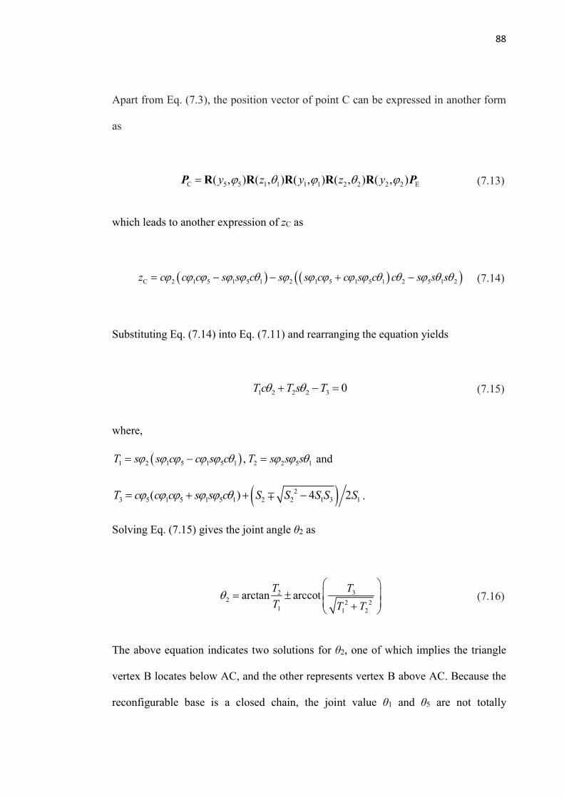
88
Apart from Eq. (7.3), the position vector of point C can be expressed in another form
as
C 5 5 1 1 1 1 2 2 2 2 E( , ) ( , ) ( , ) ( , ) ( , )y z y z y =R R R R RP P (7.13)
which leads to another expression of zC as
( ) ( )( )C 2 1 5 1 5 1 2 1 5 1 5 1 2 5 1 2z c c c s s c s s c c s c c s s s = - - + - (7.14)
Substituting Eq. (7.14) into Eq. (7.11) and rearranging the equation yields
1 2 2 2 3 0T c T s T + - = (7.15)
where,
( )1 2 1 5 1 5 1 2 2 5 1,T s s c c s c T s s s = - = and
( )23 5 1 5 1 5 1 2 2 1 3 1( ) 4 2T c c c s s c S S S S S = + + - .
Solving Eq. (7.15) gives the joint angle θ2 as
2 32 2 2
1 1 2
arctan arccotT T
T T T
= +
(7.16)
The above equation indicates two solutions for θ2, one of which implies the triangle
vertex B locates below AC, and the other represents vertex B above AC. Because the
reconfigurable base is a closed chain, the joint value θ1 and θ5 are not totally
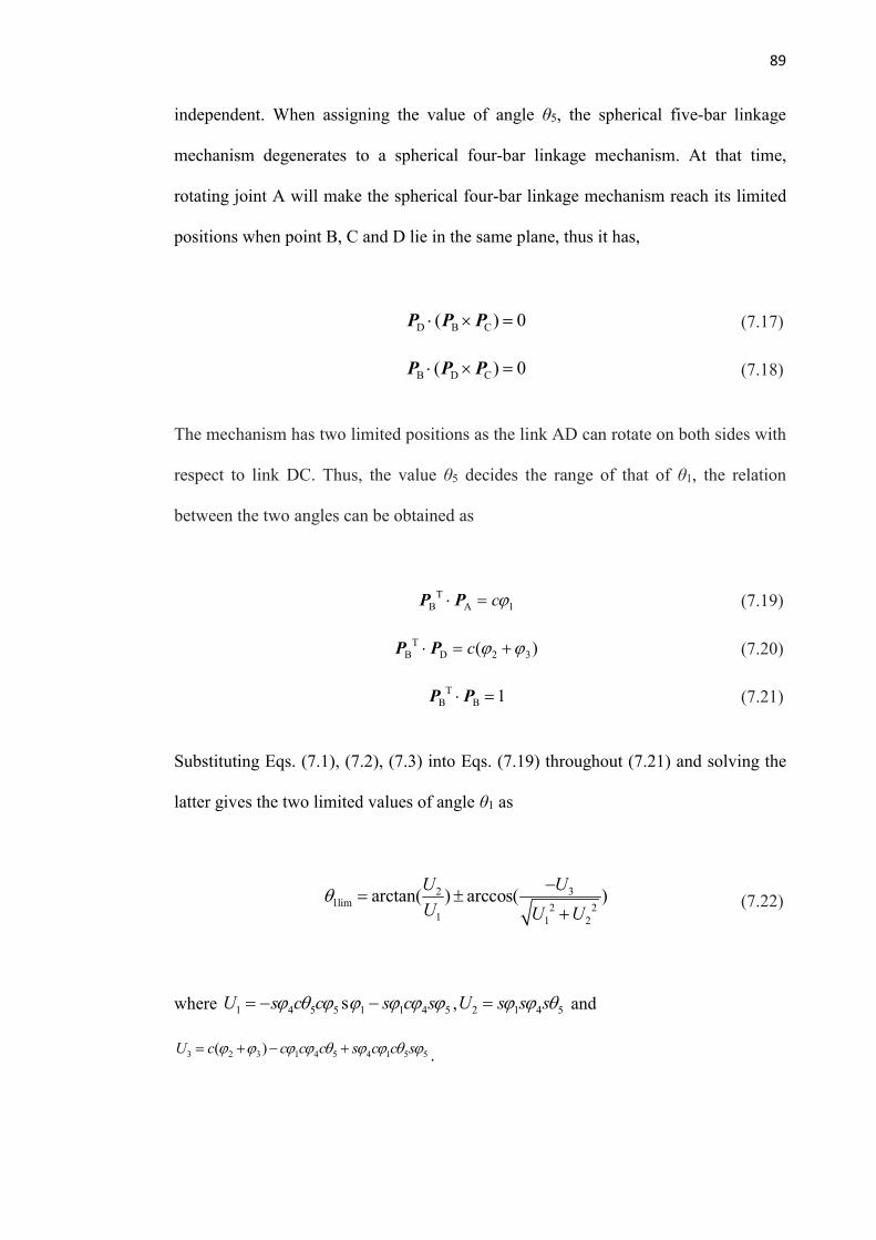
89
independent. When assigning the value of angle θ5, the spherical five-bar linkage
mechanism degenerates to a spherical four-bar linkage mechanism. At that time,
rotating joint A will make the spherical four-bar linkage mechanism reach its limited
positions when point B, C and D lie in the same plane, thus it has,
D B C( ) 0 ´ =P P P (7.17)
B D C( ) 0 ´ =P P P (7.18)
The mechanism has two limited positions as the link AD can rotate on both sides with
respect to link DC. Thus, the value θ5 decides the range of that of θ1, the relation
between the two angles can be obtained as
TB A 1c =P P (7.19)
TB D 2 3( )c = +P P (7.20)
TB B 1 =P P (7.21)
Substituting Eqs. (7.1), (7.2), (7.3) into Eqs. (7.19) throughout (7.21) and solving the
latter gives the two limited values of angle θ1 as
2 3
llim 2 21 1 2
arctan( ) arccos( )U U
U U U
-=
+ (7.22)
where 1 4 5 5 1 1 4 5sU s c c s c s = - - , 2 1 4 5U s s s = and
3 2 3 1 4 5 4 1 5 5( )U c c c c s c c s = + - + .

90
Hence the range of θ1 with respect to θ5 is
1 l 2V V (7.23)
where 2 21 2 2
1 1 2
V arctan( ) arcsin( )U U
U U U
-= -
+ and 2 3
2 2 21 1 2
V arctan( ) arccos( )U U
U U U
-= +
+.
Based on the above analysis, it can be found that given a pair of θ1 and θ5, there are four
groups of solution for θ2, θ3 and θ4 resulting in four different configurations of the base.
Motion planning is needed when controlling this mechanism because the configuration
of the spherical base is considered by the order of its inputs.
7.3.2 Position of the 3-RRS Parallel Mechanism in a Particular
Configuration of the Reconfigurable Base
A local coordinate system M'{O'-x'y'z'} is attached to the upper moving platform with
the origin O' coincided with the centroid of the equilateral triangle ∆C1C2C3 and the z'-
axis directed to point C1. The coordinates of Ai (i = 1, 2 and 3) in the global coordinate
system are given by,
1
TFA 0 0 1=P (7.24)
2 1
F FA 1 1 1 1 1 2 2 2 2 A( , ) ( , ) ( , ) ( , ) ( , ) y z y z y = R R R R RP P (7.25)
3 1
F FA 1 5 5 4 4 4 4 3 3 A( , ) ( , ) ( , ) ( , ) ( , )y z y z y = - - - - -R R R R RP P (7.26)
The coordinates of Ci in the coordinate system M' can be obtained as
91
1
TM'C 0 0 r=P (7.27)
2
T
M'C
30
2 2
rr
= -
P (7.28)
3
T
M'C
30
2 2
rr
= - -
P (7.29)
The upper moving platform C1C2C3 is an equilateral triangle as
21 2 3' ' ' 3O C O C O C r= = = . The position vector F
CiP of Ci (i = 1, 2 and 3) with
respect to global coordinate frame F is given by the transformation as follows,
F F F M'C OO' M' Ci i= + RP P P , (i = 1, 2 and 3), ( 7.30)
where FOO'P is the position vector of O' expressed in the global coordinate frame F and
FM R is the rotation matrix indicating the rotation of coordinates from coordinate frame
M' to the global coordinate frame F.
7.3.3 Forward Kinematics of the Spherical-base Integrated Parallel
Mechanism
The sequence of calculating the forward kinematics of the spherical-base integrated
mechanism is to take the configuration of the base into consideration primarily as a way
to degenerate the whole mechanism into a 3-RRS mechanism with a confirmed base
configuration, then apply the way to formulating forward kinematics of a parallel
mechanism to this simplified parallel mechanism, which is well presented in the

92
reference[66-68]. For each limb in this proposed mechanism, the local limb coordinate
system Ki {O-xKiyKizKi} (i =1, 2 and 3) is established with the origin O, zKi-axis directed
to point Ai and yKi-axis perpendicular to the plane formed by the linkage of the
reconfigurable base. In terms of Fig. 7.4, the yK2-axis is perpendicular to the plane
constructed by ∆COD.
The position vector of point Ci in the global coordinate frame can be described as
0
, 1, 2, 3
1
i i
i i
l s i
l c
= = -
KRi ik (7.31)
where ki is the position vector of point Ci expressed in the local coordinate system M5
{O-x5y5z5}, RKi describes the transformation from the local limb coordinate system to
the coordinate system M5 {O-x5y5z5} as
1
5 1 1 2 2
5 4 4 3
( , ) , 1
( , ) ( , ) ( , ) ( , ) ( , ), 2
( , ) ( , ) ( , ) ( , ), 3
xi xi xi
i yi yi yi
zi zi zi
u v w y i
u v w y z y z y i
z y z y iu v w
=
= = = - - - - =
K
R
R R R R R R
R R R R
(7.32)
The values of θ2 and θ4 can be obtained through Eqs. (7.16) and (7.12) according to the
geometry constraints of the reconfigurable base. So ki is computed by substituting θ2
and θ4 together with Eq. (7.32) into Eq. (7.31) as
( )
( )
1 1 1
1 1 1
1 1 1
1 (1 ) s
, (1 ) s , 2 and 3
1 (1 ) s
xi i i i xi i
i yi i i i yi i
zi i i i zi i
l c s w l c l v
l s w l c l v i
l c c w l c l v
- - +
= = - + = - - +
k k (7.33)

93
For calculating the forward kinematics, the angle value of joint Bi is given, hence the
length between point Ai and Ci is introduced by the following equation,
2 21 2 1 2 1,2 and 32 ,i i i i i il l l l l c i == + - (7.34)
Thus, the upper moving platform, which is connected to the limbs by spatial joints,
restricts the position of point Ci ; that is
( ) ( )T 2
1 1 3 , 1,2 and 3i i i i r i+ +- - = =k k k k (7.35)
Equation (7.35) describes the geometrical relation between the endpoints of any two
limbs. So if i = 3, then i + 1 is equal to 1. By utilizing the way to calculating forward
kinematics of the parallel mechanism introduced by Merlet [66], we can see that there
are up to 16 solutions for the fixed-base parallel mechanism. However, in this spherical-
base integrated mechanism, the number doubles as the reconfigurable base provides
two configurations for given inputs investigated in Section 7.3.1. Path planning is
necessary to get a desired configuration of the base and the moving platform.
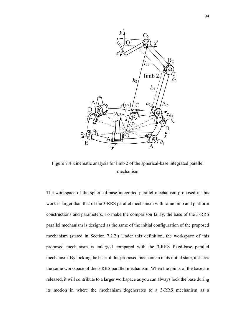
94
Figure 7.4 Kinematic analysis for limb 2 of the spherical-base integrated parallel
mechanism
The workspace of the spherical-base integrated parallel mechanism proposed in this
work is larger than that of the 3-RRS parallel mechanism with same limb and platform
constructions and parameters. To make the comparison fairly, the base of the 3-RRS
parallel mechanism is designed as the same of the initial configuration of the proposed
mechanism (stated in Section 7.2.2.) Under this definition, the workspace of this
proposed mechanism is enlarged compared with the 3-RRS fixed-base parallel
mechanism. By locking the base of this proposed mechanism in its initial state, it shares
the same workspace of the 3-RRS parallel mechanism. When the joints of the base are
released, it will contribute to a larger workspace as you can always lock the base during
its motion in where the mechanism degenerates to a 3-RRS mechanism as a

95
consequence. In other words, the workspace of the spherical-base integrated parallel
mechanism is the sum of the workspaces of its degenerated 3-RRS parallel mechanisms
with all possible base configurations.
7.4 Inverse Kinematics of the Spherical-Base Integrated
Parallel Mechanism
The inverse kinematic problem can be described as giving the position and orientation
of the upper moving platform to acquire the rotation angle of each active joint. For
simplifying the model, we assume that point Ai (i = 1, 2 and 3) is on the links of the
reconfigurable base. By decomposing the hybrid mechanism into a spherical five-bar
linkage and a 3-RRS parallel mechanism where its three limbs are mounted on the
former, the inverse kinematics of each linkage is investigated and then integrated
through the instinct geometry when connecting them. As the configurations of the
reconfigurable five-bar base play a vital role in deciding the position and orientation of
the platform, it has to be primarily considered. In this case, the procedures of obtaining
the inverse kinematics of this mechanism are divided into the following two steps:
a. Find all possible configurations of the base relying on its geometric constraints
with the platform when the position and orientation of the latter are given.
b. For considering the mechanism as a whole after decouple, the length of each
limb has to be achievable which it lies in the certain boundary.
For every possible configuration of the spherical base, it has to satisfy the geometric
condition that the plane constructed by ∆OAiBi (i = 1, 2 or 3) is perpendicular to its

96
corresponding plane constructed by the linkage of the reconfigurable base. As shown
in Fig. 7.4, ∆OA2B2 is orthogonal to ∆OBC. Denote C’i the intersection between OCi
and the surface of the sphere constructed by the spherical mechanism. In this way, the
coordinates of C’3 can be written as,
' ' ' '3 3 33 3 3 3
3 3 3
TT
C 2 2 2
1C C C C C C
C C C
x y z x y zx y z
= = + +P
The coordinates of C’3 can be acquired in another way by multiplying the rotation
matrices from the point E as,
C 5 5 4 4 4 4 3 3 3 3 E
3 3 4 5 4 4 5 3 5 4 3 4 5 4 5 4
3 3 4 5 4 4 5 3 5 4 3 4 5 4 4 5
3 3 4 3 4 4 3 4 4
( , ) ( , ) ( , ) ( , ) ( , )
( ( ) ) ( )
( ( ) ) ( )
( )
z y z y x
c s s s c c c c c s s c s c c s
c s s c c c s c s s s c c c s s
c c c s c s s s s
= - - - - -
- - + +
= + + + -
- +
R R R R RP P
'3
'3
'3
C
C
C
x
y
z
=
(7.36)
As there are only three unknowns θ4, θ5 and r3 in Eq. (7.36), the standard trigonometric
substitutions are adopted to estimate these unknown variables,
21 1
3 2 21 1
22 1
4 42 22 1
23 3
5 52 23 3
2 1,
1 1
2 1,
1 1
2 1,
1 1
r
u us c
u u
u us c
u u
u us c
u u
-= = + +
-= =+ +
-= =+ +
(7.37)
In order to estimate u2, substituting Eq. (7.38) into the equations in Eq. (7.37) results in
three quadratic equations in u2
97
21 2 2 2 3 0E u E u E+ + = (7.38)
21 2 2 2 3 0F u F u F+ + = (7.39)
21 2 2 2 3 0G u G u G+ + = (7.40)
where Ei and Fi are second-degree polynomials in u3 and u1 and Gi (i = 1, 2, 3) is the
second-degree polynomials in u1, shown in Appendix B. Sylvester Dialytic Elimination
Method [38] can be utilized here to estimate u2 from these equations. Taking Eq. (7.38)
× G1 − Eq. (7.40) × E1 and Eq. (38) × G3 − Eq. (7.40) × E3 respectively, the two linear
equation in u3 are obtained as
( ) ( )1 2 2 1 2 1 3 3 1 0E G E G u E G E G- + - = (7.41)
( ) ( )3 1 1 3 2 3 2 2 3 0E G E G u E G E G- + - = (7.42)
Combining Eq. (7.41) and Eq. (7.42) to estimate u2, we obtain,
( ) ( ) ( )2
1 3 3 1 1 2 2 1 3 2 2 3 0E G E G E G E G E G E G- + - - = (7.43)
A fourth-degree polynomial in u3 can be derived from substituting Ei and Gi (i = 1, 2,
3) into Eq. (7.43); that is,
4 3 21 3 2 3 3 3 4 3 5 0J u J u J u J u J+ + + + = (7.44)
where Ji (i = 1 to 5) is eighth-degree polynomials in u1. Taking the same method for
Eqs. (7.39) and (7.40), and writing it in the similar form with Eq. (44) as,
98
4 3 21 3 2 3 3 3 4 3 5 0H u H u H u H u H+ + + + = (7.45)
where Hi (i = 1 to 3) is eighth-degree polynomials in u1. For estimating the term 43u , we
multiply Eq. (7.44 ) by H1 and Eq. (7.45) by J1, and then take the subtraction of the two
to obtain the third-degree polynomial in u3, as follows,
( ) ( ) ( ) ( )3 22 1 1 2 3 3 1 1 3 3 4 1 1 4 3 5 1 1 5 0H J H J u H J H J u H J H J u H J H J- + - + - + - = (7.46)
Another equation of u3 can be derived from multiplying Eq. (7.44) by H2 and Eq. (7.45)
by J2, and subtracting, which yields,
( ) ( ) ( ) ( )4 22 1 1 2 3 2 3 3 2 3 2 4 4 2 3 2 5 5 2 0H J H J u H J H J u H J H J u H J H J- + - + - + - = (7.47)
Multiplying Eq. (7.45) by u3 leads to
( ) ( ) ( ) ( )4 3 22 1 1 2 3 3 1 1 3 3 4 1 1 4 3 5 1 1 5 3 0H J H J u H J H J u H J H J u H J H J u- + - + - + - = (7.48)
We write Eqs. (7.44) throughout (7.48) in matrix form as
4 3 23 3 3 3, , , ,1
Tu u u u = M 0 (7.49)
Where
1 2 3 4 5
1 2 3 4 5
2 1 1 2 3 1 1 3 4 1 1 4 5 1 1 5
2 1 1 2 2 3 3 2 2 4 4 2 2 5 5 2
2 1 1 2 3 1 1 3 4 1 1 4 5 1 1 5
0
0
0
H H H H H
J J J J J
H J H J H J H J H J H J H J H J
H J H J H J H J H J H J H J H J
H J H J H J H J H J H J H J H J
= - - - -
- - - - - - - -
M

99
Equation (7.49) is valid if and only if the determinant of M is equal to zero, which
results in a thirty-second-degree polynomial in the square of u1, as follow,
64
10
0ii
i
N u=
= (7.50)
In Eq. (7.50), Ni is only decided by the structure of the hybrid mechanism. Solving Eq.
(7.50) will obtain at most 32 pairs of solutions for u1, with each pair containing one
positive and one negative solution. The other two parameters u2 and u3 can be calculated
by substituting u1 into Eqs. (7.45) and (7.40) separately, which overall results in 64
groups of solution for u2 and u3. Thus, θ4, θ5 and r3 are solved in the Eq. (7.38) by
substituting the above parameter into these trigonometric functions. Once θ4 and θ5 are
obtained, the configuration of the spherical base is confirmed. The next step is to solve
the configuration for the limbs based on the known base configuration and moving
platform.
With explicit expressions of PAi and ki (i = 1, 2 or 3), we can move forward to obtain
the length of each limb so as to get the value of βi (i = 1, 2 or 3) in the ∆AiBiCi and
complete to solve the inverse kinematics, by the following equation,
( )2 2 21 2 1 2 1,22 an, d 3 i i i i i i ic l l l l l = - =+ (7.51)
Two solutions of βi (i = 1, 2 or 3) exist for non-singular configurations of each limb that
contribute to 8 possible states for a specific base configuration, which leads to at most
512 different configurations for the whole mechanism theoretically. The quantity of
100
possible configurations is much smaller that the theoretical number because the
solutions of the spherical base only consider the geometrical constraint of limb 3, and
these solutions need to be verified to satisfy the corresponding geometrical constraint
of limb 2, which will significantly decrease the number of solutions.
7.5 Screw Theory based Jacobian Analysis
As aforementioned, since the parallel mechanism consists of three limbs mounted on a
reconfigurable base, structure decomposition of the mechanism can be applied to
analysing the Jacobian matrix of the whole mechanism, the Jacobian analysis of the
reconfigurable base can be completed first followed by that of the parallel mechanism.
7.5.1 Jacobian Analysis for the Reconfigurable Base
The velocity of point C can be expressed as a linear combination of angular velocity of
axis OA and OB or the other linear combination of angular velocity of axis OE and OD,
C 1 A C 2 B C( ) ( ) = ´ + ´v P P P P (7.52)
C 5 E C 4 D C( ) ( ) = ´ + ´v P P P P (7.53)
Since vC is a passive variable, it should be estimated from Eqs. (7.52) and (7.53). Thus
we take right inner product on both sides of Eqs. (7.52) and (7.53) with PD, it has
D C 1 D A C 2 D B C( ) ( ) = ´ + ´P v P P P P P P (7.54)
D C 5 D E C( ) = ´P v P P P (7.55)

101
Substituting Eq. (7.55) into Eq. (7.54) yields,
D A C D E C
2 1 5
D B C D B C
( ) ( )
( ) ( )
´ ´= - +
´ ´
P P P P P P
P P P P P P (7.56)
Similarly, the angular velocity 4 can be obtained and expressed as,
B A C B E C
4 1 5
B D C B D C
( ) ( )
( ) ( )
´ ´= -
´ ´
P P P P P P
P P P P P P (7.57)
The Eqs. (7.56) and (7.57) can be expressed in matrix form as,
D A C D E C
D B C D B C1 12
B A C B E C5 54
B D C B D C
( ) ( )
( ) ( )
( ) ( )
( ) ( )
´ ´ - ´ ´ = =
´ ´ - ´ ´
P P P P P P
P P P P P PJ
P P P P P P
P P P P P P
(7.58)
Thus the angular velocity of passive joints B and D is calculated through that of active
joints A and E based on the geometric constraints of the spherical mechanism.
7.5.2 Screw-based Jacobian Analysis for the Spherical-Base
Integrated Parallel Mechanism
The screw algebra is introduced in this section for analysing the velocity of the
spherical-base integrated parallel mechanism. A screw S is a six-dimensional vector
representing instantaneous kinematic properties of a rigid body, commonly expressed
as,
T
0 0 0
0
, , , , ,x y z x y zs s s s s s+ h
= ´
s sS = =
s r s s (7.59)

102
The first three components consist of a unit vector s directing along the screw axis, as
well as the joint axis when describing a rotation. The last elements constitute s0
representing the moment of the vector s about the origin of the reference frame, and h
expresses the screw pitch, which is equal to 0 for revolute joints and ∞ for prismatic
joints, r is the position vector from the origin of the reference coordinate system to an
arbitrary point on the screw axis s.
(a) (b)
Figure 7.5 Motion screw of the spherical-base integrated parallel mechanism
The whole mechanism Jacobian can be derived from the twist of the mechanism based
on screw system notation. Fig. 7.5(a) illustrates motion screws of the spherical-base
integrated parallel mechanism. We can assume each limb as an open-loop chain
connecting the end-effector to the base, as shown in Fig. 7.5 (b). Defining Sp as the
instantaneous motion of the moving platform, the twist Sp can be derived from the linear
103
combination of each joint’s twist within the loop. Referring to Fig. 7.5(a), twist Sp can
be obtained in terms of limb 1, 2 and 3 separately as
5
1 11
p i ii
=
=S S (7.60)
5
1 2 2 21
p a b i ii
=
= + +S S S S (7.61)
5
4 5 3 31
p d e i ii
=
= + +S S S S (7.62)
Substituting Eqs. (7.56) and (7.57) into Eqs. (7.61) and (7.62) respectively leads to,
( )5
1 1 2 5 2 21
p a b b i ii
m m =
= - + +S S S S S (7.63)
( )5
3 1 5 4 2 21
p d e d i ii
m m =
= + - +S S S S S (7.64)
where D A C1
D B C
( )
( )m
´=
´
P P P
P P P, D E C
2
D B C
( )
( )m
´=
´
P P P
P P P, B A C
3
B D C
( )
( )m
´=
´
P P P
P P P and
B E C4
B D C
( )
( )m
´=
´
P P P
P P P.
According to [65], we know that the revolute-spherical screws dyad locate in a four-
dimensional vector space. So the reciprocal screws form a two-system with zero pitch.
Let 1riS and 2
riS (i = 1, 2 and 3) denote a two-system of screws that is reciprocal to the
four-system of screws Si2 to Si5 (i = 1, 2 and 3) of the ith limb. Performing the reciprocal
product of both sides of Eqs. (7.60), (7.63) and (7.64) with reciprocal screw 1riS and
2riS gives six linear equations, which can be expressed in matrix form as,
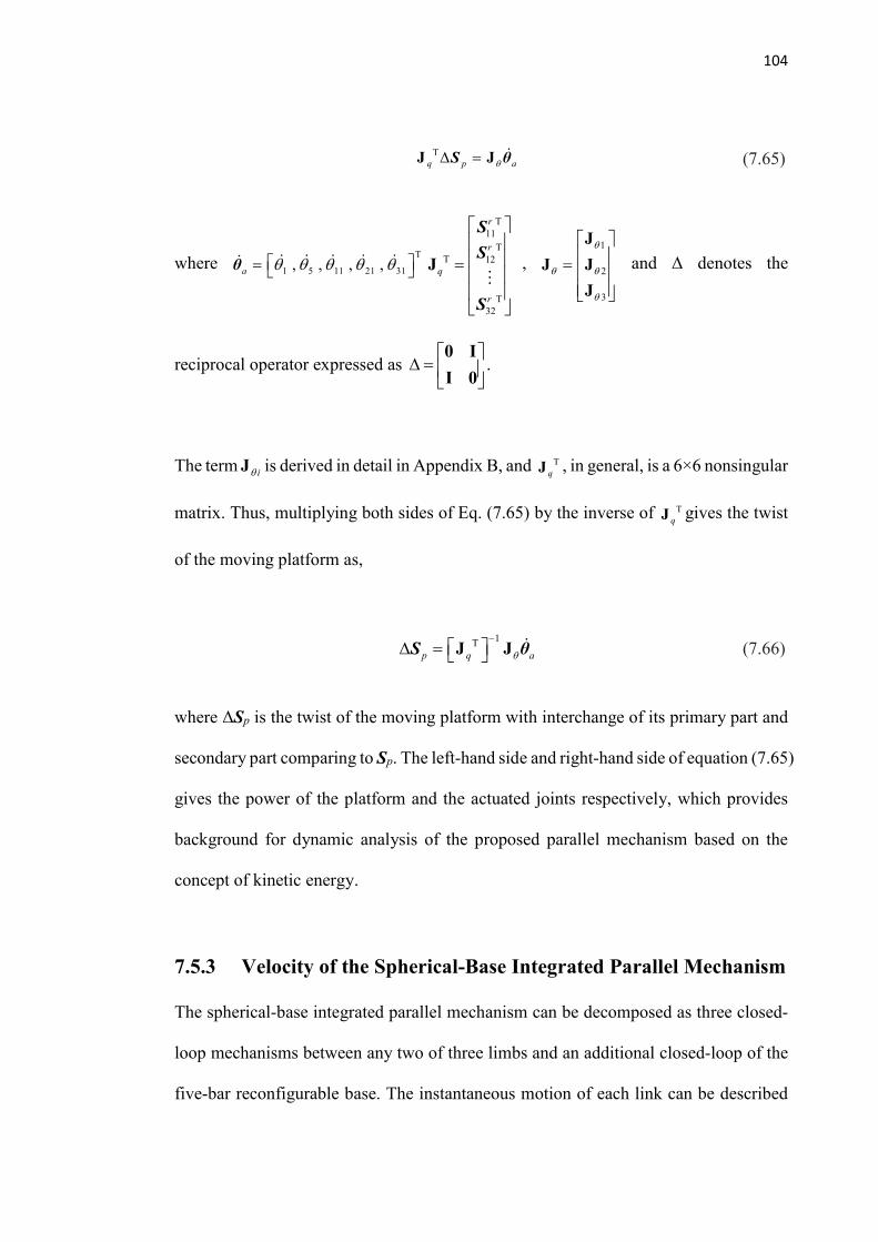
104
T
q p aD =J JS θ (7.65)
where T
1 5 11 21 31, , , ,a = θ
T11
TT 12
T32
r
r
q
r
=
J
S
S
S
,
1
2
3
=
J
J J
J
and Δ denotes the
reciprocal operator expressed as
D =
0 I
I 0.
The term iJ is derived in detail in Appendix B, and TqJ , in general, is a 6×6 nonsingular
matrix. Thus, multiplying both sides of Eq. (7.65) by the inverse of TqJ gives the twist
of the moving platform as,
1T
p q a
- D = J JS θ (7.66)
where ΔSp is the twist of the moving platform with interchange of its primary part and
secondary part comparing to Sp. The left-hand side and right-hand side of equation (7.65)
gives the power of the platform and the actuated joints respectively, which provides
background for dynamic analysis of the proposed parallel mechanism based on the
concept of kinetic energy.
7.5.3 Velocity of the Spherical-Base Integrated Parallel Mechanism
The spherical-base integrated parallel mechanism can be decomposed as three closed-
loop mechanisms between any two of three limbs and an additional closed-loop of the
five-bar reconfigurable base. The instantaneous motion of each link can be described
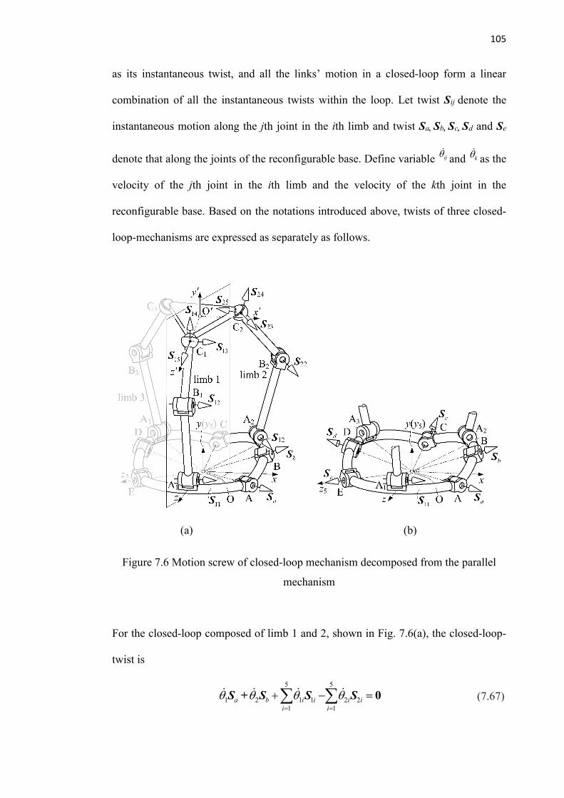
105
as its instantaneous twist, and all the links’ motion in a closed-loop form a linear
combination of all the instantaneous twists within the loop. Let twist Sij denote the
instantaneous motion along the jth joint in the ith limb and twist Sa, Sb, Sc, Sd and Se
denote that along the joints of the reconfigurable base. Define variable ij
and k
as the
velocity of the jth joint in the ith limb and the velocity of the kth joint in the
reconfigurable base. Based on the notations introduced above, twists of three closed-
loop-mechanisms are expressed as separately as follows.
(a) (b)
Figure 7.6 Motion screw of closed-loop mechanism decomposed from the parallel
mechanism
For the closed-loop composed of limb 1 and 2, shown in Fig. 7.6(a), the closed-loop-
twist is
5 5
1 2 1 1 2 21 1
a b i i i ii i
= =
+ - = 0S + S S S (7.67)
106
For limb 2 and 3, the closed-loop-twist is
5 5
3 2 2 3 31 1
c i i i ii i
= =
+ - = 0S S S (7.68)
And for limb 3 and 1, the closed-loop-twist is
5 5
4 5 3 3 1 11 1
d e i i i ii i
= =
+ - = 0S + S S S (7.69)
Further, the closed-loop-twist of the reconfigurable base, shown in Fig. 7.6(b) is
1 2 3 4 5a b c d e + + + + = 0S S S S S (7.70)
In each decomposed closed-loop-mechanism, only part of all the joints are active, which
can be separated from the rest passive joints in the twists given in Eqs. (7.67) throughout
(7.70) as,
5 5
1 11 11 21 21 2 1 1 2 22 2
a b i i i ii i
= =
+ - = - - + S S S S S S (7.71)
5 5
21 21 31 31 3 2 2 3 32 2
c i i i ii i
= =
- = - - + S S S S S (7.72)
5 5
5 31 31 11 11 4 3 3 1 12 2
e d i i i ii i
= =
+ - = - - + S S S S S S (7.73)
1 5 2 3 4a e b c d + = - - -S S S S S (7.74)
The Eqs. (7.71) to (7.74) can be expressed in a matrix form that indicates the
relationship between velocity of the active joints and that passive joints as,
107
a a p p=J Jθ θ (7.75)
where aθ and pθ denote the velocity vectors of active joints and passive joints as,
T
2 3 4 12 13 14 15 35, , , , , , , ... ,P = θ , aJ and pJ denote the active-Jacobian
matrix and passive-Jacobian matrix respectively as
1 11 21
21 31
5 11 31
1 5
a
- - =
-
J
S 0 S S 0
0 0 0 S S
0 S S 0 S
S S 0 0 0
and
2 1 2
3 2 3
4 1 3
2 3 4
p p
p p
p
p p
- - - - =
- - - - -
J J
J JJ
J J
S 0 0 0
0 S 0 0
0 0 S 0
S S S 0 0 0
where 2 3 4 5 , 1 , 2 and 3pi i i i i i= =J S S S S .
The above Jacobian matrixes can be used for singularity and dexterity analysis of the
proposed integrated parallel mechanism.
7.6 Conclusions
In this chapter, a parallel mechanism with a reconfigurable base was for the first time
presented based on the manipulation of rigid objects using a Metamorphic hand. The
structure of the proposed mechanism was presented followed by the geometric
constraint analysis.
Through decomposing the mechanism into a typical 3RRS parallel mechanism and a
spherical five-bar linkage, the kinematics was investigated, leading to closed-form
108
solutions for forward and inverse kinematics. Then, the screw-based Jacobian was
utilized to establish the relationship between active joints and passive joints through the
reciprocal product of twists and wrenches. The kinematics study demonstrated that this
novel spherical-base integrated parallel manipulator had an enlarged workspace
compared with conventional parallel mechanisms.
109
Chapter 8 Screw Embedded Jacobian and
Exponential Mapping of Grasp Affordability
with a Reconfigurable Palm
8.1 Introduction
This chapter presents the kinematics and grasp constraint and affordance of a newly
designed mobile manipulator with a three-fingered Metamorphic robotic hand.
Structure design of the mobile manipulator, which contains a Robotino 3.0, a
customised robot arm and a three-fingered Metamorphic hand, is presented. Using
mechanism decomposition, kinematics of the manipulator is formulated based on
product-of-exponentials method and kinematics of the Metamorphic hand is
investigated leading to the construction of grasp constraint providing a theoretical
background for measuring grasp quality of the grasps predicted by the grasp-affordance
model.
Further, the relation of the grasp-affordance model to the manipulator and hand
kinematics with the associated grasp constraint are indicated linking the manipulator
kinematics with the grasp-affordance model for object manipulation. The mobile
manipulator proposed in this work is to be used for toys tidying up in a child’s room
with extended applications to the field of service robot in clutter clearing.
110
8.2 Structure of a Mobile Manipulator with a
Metamorphic Robotic Hand
A low cost customised mobile manipulator is designed in this work as illustrated in Fig.
8.1. It contains a mobile platform, i.e. Robotino 3.0 developed by FestoTM, a customised
5-DOF robot arm, a customized 2-DOF wrist and a three-fingered Metamorphic robotic
hand. The commercialized mobile robot Robotino 3.0 forms the base of the manipulator
permitting it to move, normally translations along and directions and rotation about Z-
axis (see Fig. 8.1), freely around specified working environment and locate the
manipulator at a desired task position. It contains a vision system and a collision-
avoiding contour controller consisting of nine distance sensors. The 5-DOF robot arm
is a light-weight arm which is specially designed for the purpose of carrying the
proposed Metamorphic hand with an additional 2-DOF wrist. The wrist inherits the
structure of a universal joint, and connects the three-fingered Metamorphic hand to the
robot arm. The Metamorphic robotic hand consists of a reconfigurable palm and three
fingers which are evenly distributed around the palm. Each of the three fingers has two
phalanges connected by two parallel revolute joints providing two degrees of freedom.
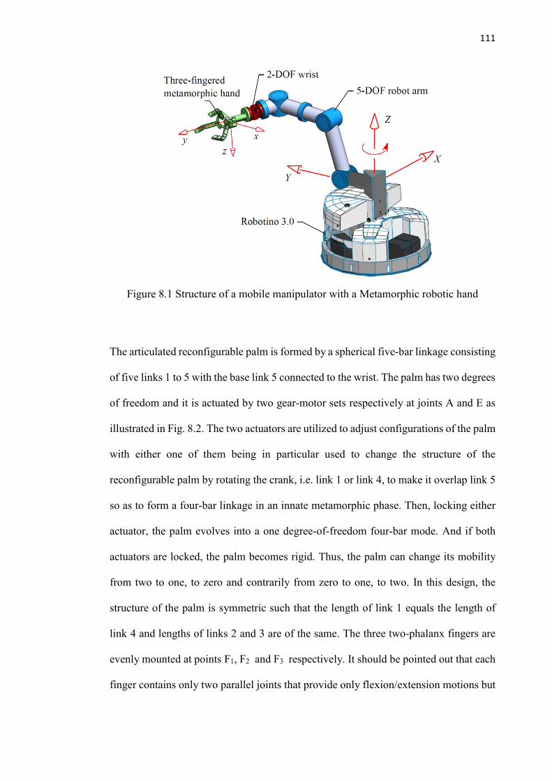
111
Figure 8.1 Structure of a mobile manipulator with a Metamorphic robotic hand
The articulated reconfigurable palm is formed by a spherical five-bar linkage consisting
of five links 1 to 5 with the base link 5 connected to the wrist. The palm has two degrees
of freedom and it is actuated by two gear-motor sets respectively at joints A and E as
illustrated in Fig. 8.2. The two actuators are utilized to adjust configurations of the palm
with either one of them being in particular used to change the structure of the
reconfigurable palm by rotating the crank, i.e. link 1 or link 4, to make it overlap link 5
so as to form a four-bar linkage in an innate metamorphic phase. Then, locking either
actuator, the palm evolves into a one degree-of-freedom four-bar mode. And if both
actuators are locked, the palm becomes rigid. Thus, the palm can change its mobility
from two to one, to zero and contrarily from zero to one, to two. In this design, the
structure of the palm is symmetric such that the length of link 1 equals the length of
link 4 and lengths of links 2 and 3 are of the same. The three two-phalanx fingers are
evenly mounted at points F1, F2 and F3 respectively. It should be pointed out that each
finger contains only two parallel joints that provide only flexion/extension motions but
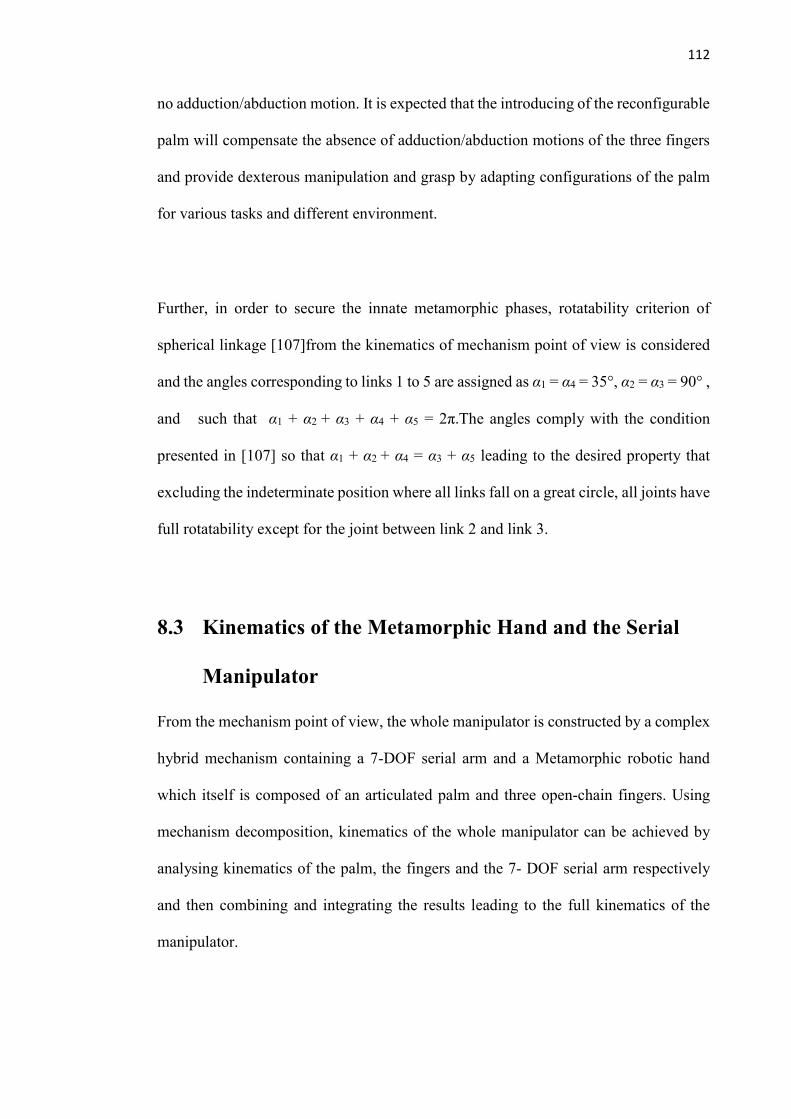
112
no adduction/abduction motion. It is expected that the introducing of the reconfigurable
palm will compensate the absence of adduction/abduction motions of the three fingers
and provide dexterous manipulation and grasp by adapting configurations of the palm
for various tasks and different environment.
Further, in order to secure the innate metamorphic phases, rotatability criterion of
spherical linkage [107]from the kinematics of mechanism point of view is considered
and the angles corresponding to links 1 to 5 are assigned as α1 = α4 = 35°, α2 = α3 = 90° ,
and such that α1 + α2 + α3 + α4 + α5 = 2π.The angles comply with the condition
presented in [107] so that α1 + α2 + α4 = α3 + α5 leading to the desired property that
excluding the indeterminate position where all links fall on a great circle, all joints have
full rotatability except for the joint between link 2 and link 3.
8.3 Kinematics of the Metamorphic Hand and the Serial
Manipulator
From the mechanism point of view, the whole manipulator is constructed by a complex
hybrid mechanism containing a 7-DOF serial arm and a Metamorphic robotic hand
which itself is composed of an articulated palm and three open-chain fingers. Using
mechanism decomposition, kinematics of the whole manipulator can be achieved by
analysing kinematics of the palm, the fingers and the 7- DOF serial arm respectively
and then combining and integrating the results leading to the full kinematics of the
manipulator.
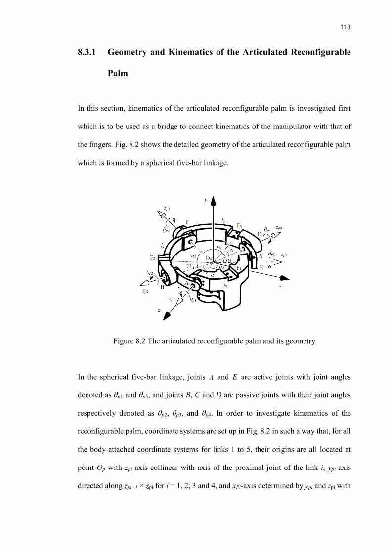
113
8.3.1 Geometry and Kinematics of the Articulated Reconfigurable
Palm
In this section, kinematics of the articulated reconfigurable palm is investigated first
which is to be used as a bridge to connect kinematics of the manipulator with that of
the fingers. Fig. 8.2 shows the detailed geometry of the articulated reconfigurable palm
which is formed by a spherical five-bar linkage.
Figure 8.2 The articulated reconfigurable palm and its geometry
In the spherical five-bar linkage, joints A and E are active joints with joint angles
denoted as θp1 and θp5, and joints B, C and D are passive joints with their joint angles
respectively denoted as θp2, θp3, and θp4. In order to investigate kinematics of the
reconfigurable palm, coordinate systems are set up in Fig. 8.2 in such a way that, for all
the body-attached coordinate systems for links 1 to 5, their origins are all located at
point Op with zpi-axis collinear with axis of the proximal joint of the link i, ypi-axis
directed along zpi+1 × zpi for i = 1, 2, 3 and 4, and xPi-axis determined by ypi and zpi with
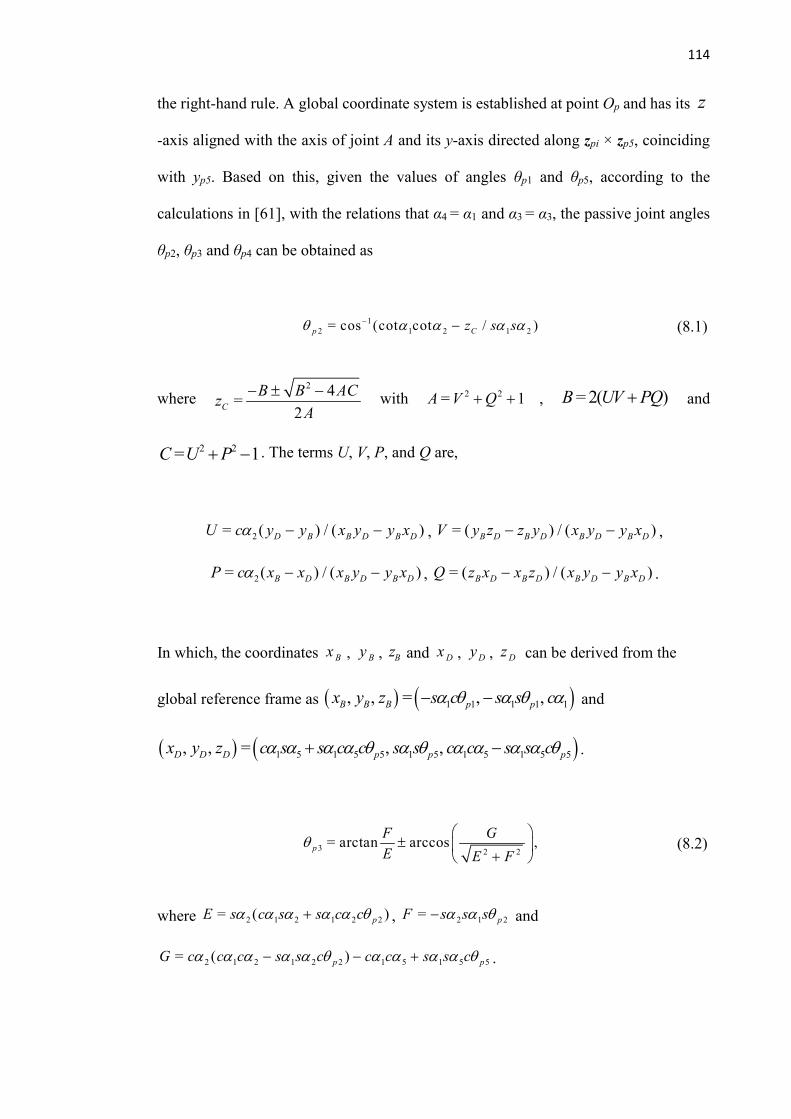
114
the right-hand rule. A global coordinate system is established at point Op and has its z
-axis aligned with the axis of joint A and its y-axis directed along zpi × zp5, coinciding
with yp5. Based on this, given the values of angles θp1 and θp5, according to the
calculations in [61], with the relations that α4 = α1 and α3 = α3, the passive joint angles
θp2, θp3 and θp4 can be obtained as
1
2 1 2 1 2= cos (cot cot / )p Cz s s - - (8.1)
where 2 4
=2
C
B B ACz
A
- - with 2 2= 1A V Q+ + , = 2( )B UV PQ+ and
2 2= 1C U P+ - . The terms U, V, P, and Q are,
2= ( ) / ( )D B B D B DU c y y x y y x - - , = ( ) / ( )B D B D B D B DV y z z y x y y x- - ,
2= ( ) / ( )B D B D B DP c x x x y y x - - , = ( ) / ( )B D B D B D B DQ z x x z x y y x- - .
In which, the coordinates Bx , By , Bz and Dx , Dy , Dz can be derived from the
global reference frame as ( ) ( )1 1 1 1 1, , = , ,B B B p px y z s c s s c - - and
( ) ( )1 5 1 5 5 1 5 1 5 1 5 5, , = , ,D D D p p px y z c s s c c s s c c s s c + - .
3 2 2= arctan arccos ,p
F G
E E F
+ (8.2)
where 2 1 2 1 2 2= ( )pE s c s s c c + , 2 1 2= pF s s s - and
2 1 2 1 2 2 1 5 1 5 5= ( )p pG c c c s s c c c s s c - - + .

115
4 2 2= arctan arccos .p
M Nand
L M L
+ (8.3)
with 2 1 5 1 5 5= ( )pL s s s c s c + , 2 5 5= pM s s s - and
22 1 5 1 5 5= ( ) ( 4 ) / 2pN c c c s s c B B AC A - + - .
Thus this section presents geometry and kinematics of the articulated reconfigurable
palm which lays a foundation for linking the kinematics of the robot arm and the fingers
leading to the full kinematics of the whole manipulator.
8.3.2 Kinematics of the 7-DOF Serial Robot
Treating the robot arm and wrist together as a 7-DOF serial robot, its kinematics can be
formulated with product-of-exponentials representation as follows.
The geometry of the serial robot is shown in Fig. 8.3. Lengths of the links are denoted
as αi (i = 1, 2, …, 6) and let θi ( i = 1, 2, …, 7) corresponds to the fully extended
configuration in which zero position (or reference configuration) of the 7-DOF serial
robot is defined together with a fixed reference frame {Om} and an end-effector frame
{Op} attached respectively to the Robotino and the palm of the Metamorphic robotic
hand. Further, the direction of positive rotation for each joint is defined as indicated in
Fig. 8.3.
116
Figure 8.3 Geometry of the mobile manipulator in the reference position.
Using product-of-exponential formula [96][108], the forward kinematics of the
proposed 7-DOF serial Robot has the form,
[ ] [ ] [ ] [ ][ ] [ ] [ ]3 3 5 5 6 6 7 71 1 2 2 4 4= ,O O Om p p
e e e e e e e
T MS S S SS S S
(8.4)
where Si = (ωi, vi) (i = 1, 2, …, 7) is the twist of the ith joint and MOp is the position
vector of point Op, both presented in the zero configuration in the fixed frame. The term
MOp can be directly obtained from Fig. 8.3 as
6
=1
1 0 0 0
0 1 0= .
0 0 1 0
0 0 0 1
iiOp
a
M (8.5)
Referring to Fig. 8.3, in the reference configuration, screw axis of joint 1 is
( )1 1= = 1, 0, 0-ω s . To determine v1, we pick any arbitrary point r1 that lies on the axis
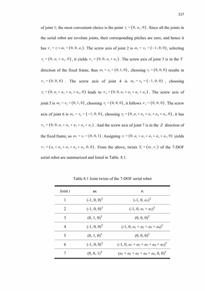
117
of joint 1; the most convenient choice is the point ( )1 1= 0, , 0r a . Since all the joints in
the serial robot are revolute joints, their corresponding pitches are zero, and hence it
has ( )1 1 1 1= = 0, 0,r a ´ . The screw axis of joint 2 is ( )2 2= = 1, 0, 0s - , selecting
( )2 1 2= 0, , 0r a a+ , it yields ( )2 1 2= 0, 0, a a + . The screw axis of joint 3 is in the Y
direction of the fixed frame, thus ( )3 3= = 0, 1, 0s , choosing ( )3 = 0, 0, 0r results in
( )3 = 0, 0, 0 . The screw axis of joint 4 is ( )4 4= = 1, 0, 0s - , choosing
( )4 1 2 3 4= 0, , 0r a a a a+ + + leads to ( )4 1 2 3 4= 0, 0, a a a a + + + . The screw axis of
joint 5 is ( )5 5= = 0, 1, 0s , choosing ( )5 = 0, 0, 0r , it follows ( )5 = 0, 0, 0 . The screw
axis of joint 6 is ( )6 6= = 1, 0, 0s - , choosing ( )6 1 2 3 4 5= 0, , 0r a a a a a+ + + + , it has
( )6 1 2 3 4 5= 0, 0, a a a a a + + + + . And the screw axis of joint 7 is in the Z direction of
the fixed frame, so ( )7 7= = 0, 0, 1s . Assigning ( )7 1 2 3 4 5= 0, , 0r a a a a a+ + + + yields
( )7 1 2 3 4 5= , 0, 0a a a a a + + + + . From the above, twists ( )= ,i i iS of the 7-DOF
serial robot are summarized and listed in Table. 8.1.
Table 8.1 Joint twists of the 7-DOF serial robot
Joint i ωi vi
1 (-1, 0, 0)T (-1, 0, α1)T
2 (-1, 0, 0)T (-1, 0, α1 + α2)T
3 (0, 1, 0)T (0, 0, 0)T
4 (-1, 0, 0)T (-1, 0, α1 + α2 + α5 + α4)T
5 (0, 1, 0)T (0, 0, 0)T
6 (-1, 0, 0)T (-1, 0, α1 + α2 + α5 + α4 + α5)T
7 (0, 0, 1)T (α1 + α2 + α5 + α4 + α5, 0, 0)T
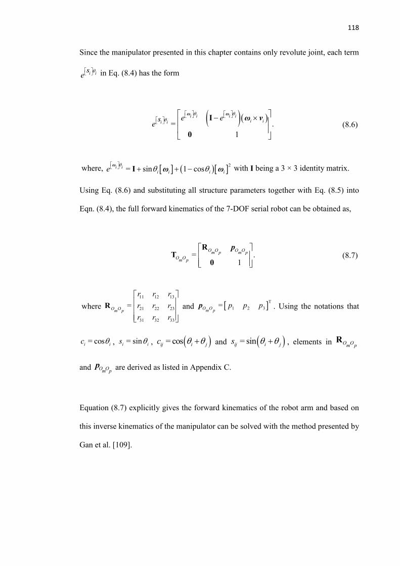
118
Since the manipulator presented in this chapter contains only revolute joint, each term
i ie
S in Eq. (8.4) has the form
( )( )
= .
1
i i i ii ii i
e ee
- ´
I
0
ω ω
S ω ν (8.6)
where, ( ) 2= sin 1 cosi ii i i ie
+ + -Iω
ω ω with I being a 3 × 3 identity matrix.
Using Eq. (8.6) and substituting all structure parameters together with Eq. (8.5) into
Eqn. (8.4), the full forward kinematics of the 7-DOF serial robot can be obtained as,
= .1
O O O Om p m pO Om p
RT
0
p (8.7)
where
11 12 13
21 22 23
31 32 33
=O Om p
r r r
r r r
r r r
R and T
1 2 3=O Om pp p pp . Using the notations that
= cosi ic , = sini is , ( )= cosij i jc + and ( )= sinij i js + , elements in O Om pR
and O Om pp are derived as listed in Appendix C.
Equation (8.7) explicitly gives the forward kinematics of the robot arm and based on
this inverse kinematics of the manipulator can be solved with the method presented by
Gan et al. [109].
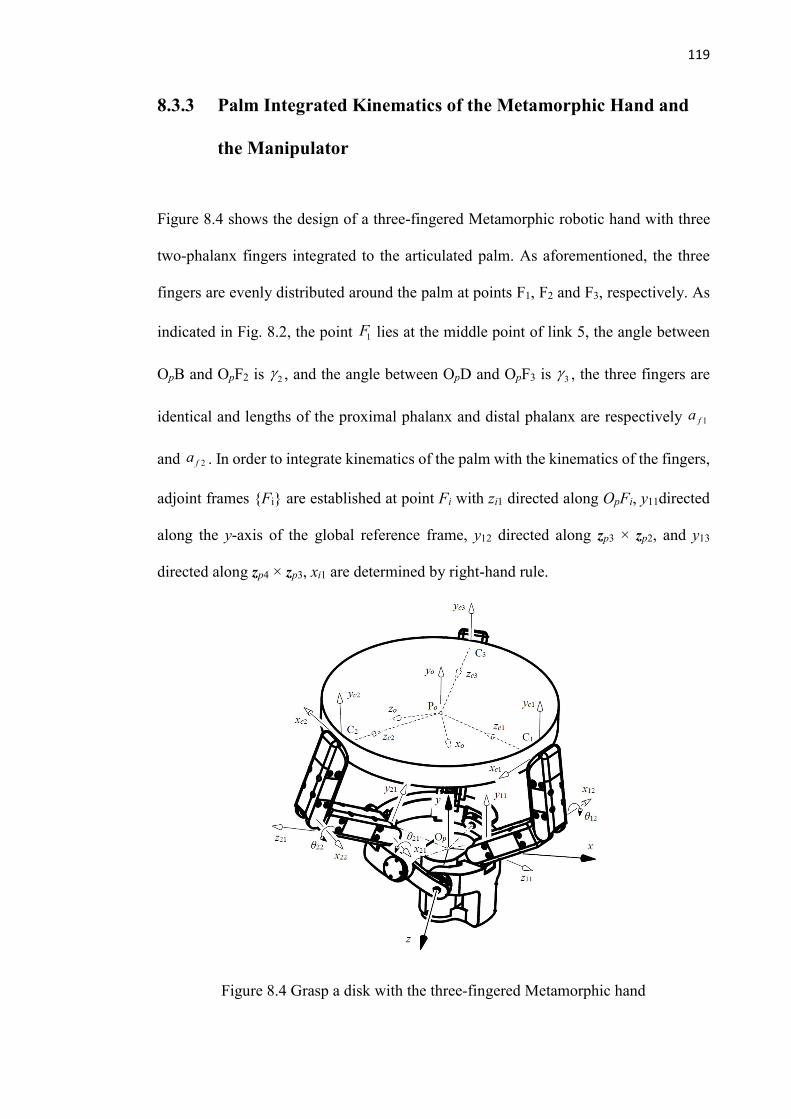
119
8.3.3 Palm Integrated Kinematics of the Metamorphic Hand and
the Manipulator
Figure 8.4 shows the design of a three-fingered Metamorphic robotic hand with three
two-phalanx fingers integrated to the articulated palm. As aforementioned, the three
fingers are evenly distributed around the palm at points F1, F2 and F3, respectively. As
indicated in Fig. 8.2, the point 1F lies at the middle point of link 5, the angle between
OpB and OpF2 is 2 , and the angle between OpD and OpF3 is 3 , the three fingers are
identical and lengths of the proximal phalanx and distal phalanx are respectively 1fa
and 2fa . In order to integrate kinematics of the palm with the kinematics of the fingers,
adjoint frames {Fi} are established at point Fi with zi1 directed along OpFi, y11directed
along the y-axis of the global reference frame, y12 directed along zp3 × zp2, and y13
directed along zp4 × zp3, xi1 are determined by right-hand rule.
Figure 8.4 Grasp a disk with the three-fingered Metamorphic hand
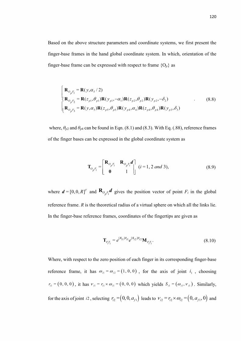
120
Based on the above structure parameters and coordinate systems, we first present the
finger-base frames in the hand global coordinate system. In which, orientation of the
finger-base frame can be expressed with respect to frame {Op} as
51
1 1 1 1 2 2 2 22
5 5 5 4 4 4 4 3 33
= ( , / 2)
= ( , ) ( , ) ( , ) ( , ) .
= ( , ) ( , ) ( , ) ( , ) ( , )
O Fp
O F p p p p p pp
O F p p p p p pp
y
z y z y
y z y z y
- -
R R
R R R R R
R R R R R R
(8.8)
where, θp2 and θp4 can be found in Eqn. (8.1) and (8.3). With Eq. (.88), reference frames
of the finger bases can be expressed in the global coordinate system as
= ( = 1, 2 3),1
O F O Fp i p iO Fp i
i and
R RT
0
d (8.9)
where = [0,0, ]TRd and O Fp iR d gives the position vector of point Fi in the global
reference frame. R is the theoretical radius of a virtual sphere on which all the links lie.
In the finger-base reference frames, coordinates of the fingertips are given as
[ ] [ ]1 1 2 2= .i i i i
F T F Ti i i ie e
T M
S S (8.10)
Where, with respect to the zero position of each finger in its corresponding finger-base
reference frame, it has ( )1 2= = 1, 0, 0i i , for the axis of joint 1i , choosing
( )1 = 0, 0, 0ir , it has ( )1 1 1= = 0, 0, 0i i ir ´ which yields ( )1 1 1= ,i i iS . Similarly,
for the axis of joint 2i , selecting ( )2 1= 0, 0,i fr a leads to ( )2 2 2 1= = 0, , 0i i i fr a ´ and
121
further to ( )2 2 2= ,i i iS . Further, in the finger reference configuration, there is
= ( , )FT FTi i i iM I p with I being a 3 by 3 identity matrix and 1 2=(0, 0, )FT f fi i
p a a+ .
Integrating the finger kinematics with the palm kinematics, the full kinematics of the
three-fingered Metamorphic robotic hand can be presented in the hand global
coordinate system as
= , ( =1, 2 3),O T O F FTp i p i i ii andT T T (8.11)
and subsequently in the manipulator global coordinate system as
= , ( =1, 2 3),O T O O O F F Tm i m p p i i ii andT T T T (8.12)
Eq. (8.12) presents the integrated full kinematics for the proposed manipulator and Eqs.
(8.11) and (8.12) provides background for further workspace, manipulability and
dexterity analysis of the proposed Metamorphic hand and the mobile manipulator.
Inverse kinematics of the proposed Metamorphic hand can be solved with the method
provided by Gao et al. [110]. Based on the hand kinematics, grasp constraint of the
robotic hand can be constructed.
8.4 Metamorphic Hand based Grasp Constraints
Based on the above hand kinematics, grasp constraint of the Metamorphic hand is
formulated in this section laying theoretical approach for measuring the grasps
predicted by grasp-affordance model from learning processor in the virtual environment
for a specified object.
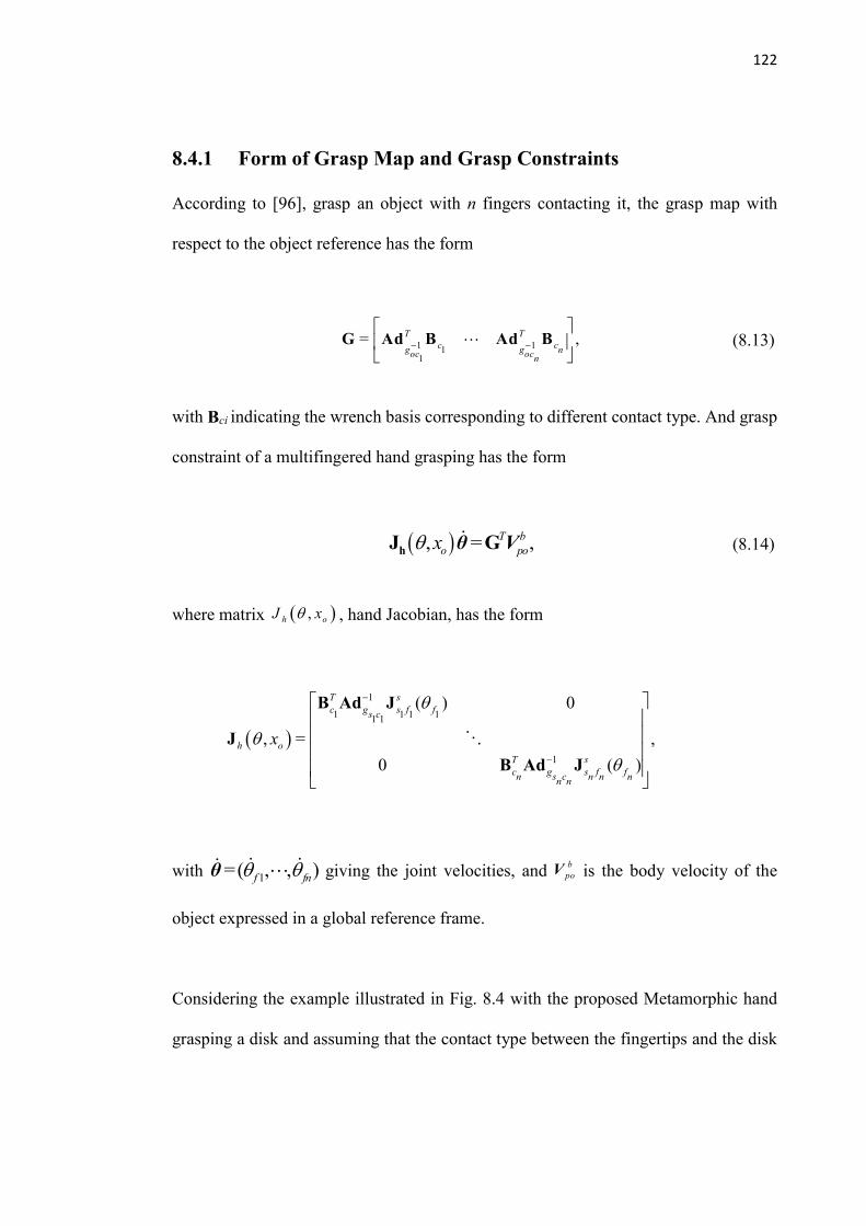
122
8.4.1 Form of Grasp Map and Grasp Constraints
According to [96], grasp an object with n fingers contacting it, the grasp map with
respect to the object reference has the form
1 111
= ,T Tc cg g noc ocn
- -
G Ad B Ad B (8.13)
with Bci indicating the wrench basis corresponding to different contact type. And grasp
constraint of a multifingered hand grasping has the form
( ), = ,T bo poxhJ Gθ V (8.14)
where matrix ( ),h oJ x , hand Jacobian, has the form
( )
1
1 1 1 11 1
1
( ) 0
, = ,
0 ( )
T sc g s f fs c
h o
T sc g s f fn s c n n nn n
x
-
-
B Ad J
J
B Ad J
with 1=( , , )f fn θ giving the joint velocities, and b
poV is the body velocity of the
object expressed in a global reference frame.
Considering the example illustrated in Fig. 8.4 with the proposed Metamorphic hand
grasping a disk and assuming that the contact type between the fingertips and the disk
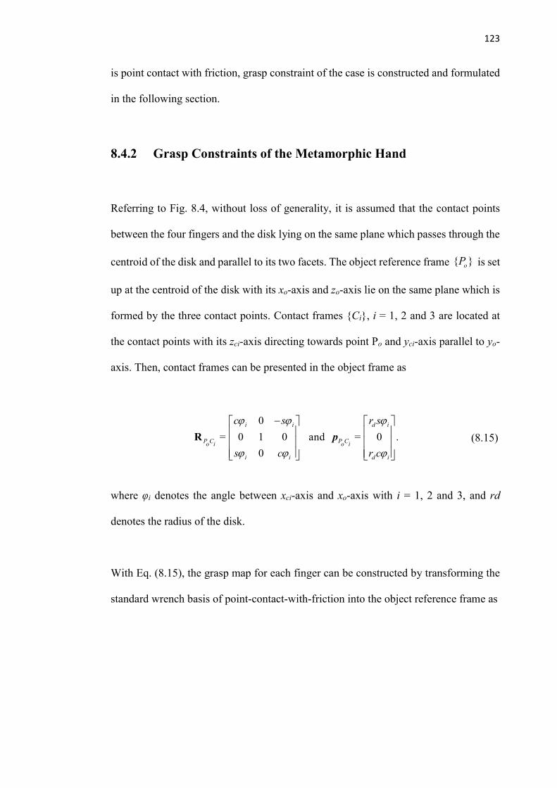
123
is point contact with friction, grasp constraint of the case is constructed and formulated
in the following section.
8.4.2 Grasp Constraints of the Metamorphic Hand
Referring to Fig. 8.4, without loss of generality, it is assumed that the contact points
between the four fingers and the disk lying on the same plane which passes through the
centroid of the disk and parallel to its two facets. The object reference frame { }oP is set
up at the centroid of the disk with its xo-axis and zo-axis lie on the same plane which is
formed by the three contact points. Contact frames {Ci}, i = 1, 2 and 3 are located at
the contact points with its zci-axis directing towards point Po and yci-axis parallel to yo-
axis. Then, contact frames can be presented in the object frame as
0
= 0 1 0 and = 0 .
0
i i d i
P C P Co i o i
i i d i
c s r s
s c r c
-
R p (8.15)
where φi denotes the angle between xci-axis and xo-axis with i = 1, 2 and 3, and rd
denotes the radius of the disk.
With Eq. (8.15), the grasp map for each finger can be constructed by transforming the
standard wrench basis of point-contact-with-friction into the object reference frame as
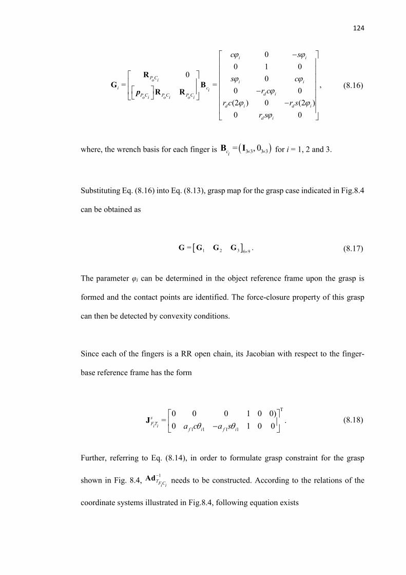
124
0
0 1 00 0
= = ,0 0
(2 ) 0 (2 )
0 0
i i
P Co i i i
i cid iP C P C P Co i o i o i
d i d i
d i
c s
s c
r c
r c r s
r s
-
-
-
R
G BR Rp
(8.16)
where, the wrench basis for each finger is ( )3 3 3 3= , 0ci ´ ´B I for i = 1, 2 and 3.
Substituting Eq. (8.16) into Eq. (8.13), grasp map for the grasp case indicated in Fig.8.4
can be obtained as
1 2 3 6 9= .
´G G G G (8.17)
The parameter φi can be determined in the object reference frame upon the grasp is
formed and the contact points are identified. The force-closure property of this grasp
can then be detected by convexity conditions.
Since each of the fingers is a RR open chain, its Jacobian with respect to the finger-
base reference frame has the form
T
1 1 1 1
0 0 0 1 0 0)= .
0 1 0 0sF Ti i
f i f ia c a s
-
J (8.18)
Further, referring to Eq. (8.14), in order to formulate grasp constraint for the grasp
shown in Fig. 8.4, 1
TF Ci i
-Ad needs to be constructed. According to the relations of the
coordinate systems illustrated in Fig.8.4, following equation exists

125
1 1 1 1= .T T T TFC P C O P F Pi i o i p o i o
- - - -Ad Ad Ad Ad (8.19)
In the object reference frame, the first term on the right-hand side of Eq. (8.19) can be
written as
1 = .
0
T TP C P C P Co i o i o i
TP C To iP Co i
- -
R RAd
R
p (8.20)
Substituting Eq. (8.15) into Eq. (8.20) yields
1
0 0 (2 ) 0
0 1 0 0
0 0 (2 ) 0= .
0 0 0 0
0 0 0 0 1 0
0 0 0 0
i i d i
d i d i
i i d i
TP Co i i i
i i
c s r c
r c r s
s c r s
c s
s c
-
- - -
-
Ad (8.21)
We assume that with respect to the hand global reference frame {Op}, orientation and
position of the object reference frame, which can be obtained from the virtual
environment of the grasp affordance model, are
= ,O Pp o
c c c s s s c c s c s s
s c s s s c c s s c c s
s c s c c
- + + - -
R (8.22)
and
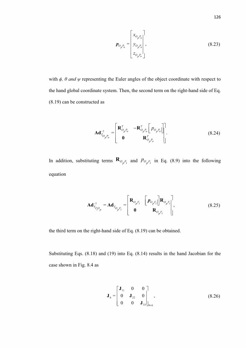
126
= ,
O Pp o
O P O Pp o p o
O Pp o
x
y
z
p (8.23)
with ϕ, θ and ψ representing the Euler angles of the object coordinate with respect to
the hand global coordinate system. Then, the second term on the right-hand side of Eq.
(8.19) can be constructed as
1 = .
T TO P O P O Pp o p o p o
TO P Tp oO Pp o
p-
-
R RAd
0 R (8.24)
In addition, substituting terms O Fp iR and O Fp i
p in Eq. (8.9) into the following
equation
1 = = ,
O F O F O Fp i p i p iT TF O O Fi p p i
O Fp i
-
R RAd Ad
0 R
p (8.25)
the third term on the right-hand side of Eq. (8.19) can be obtained.
Substituting Eqs. (8.18) and (19) into Eq. (8.14) results in the hand Jacobian for the
case shown in Fig. 8.4 as
11
22
33 9 6
0 0
= 0 0 ,
0 0h
´
J
J J
J
(8.26)
127
where, for i = 1, 2 and 3, the 3×2 sub-matrix Jii has the form
1= ,T sii C T F Ti F C i ii i
-J B Ad J
which can be obtained through symbolic computer program system such as MatlabTM
upon all the essential variables are given.
The grasp map and the grasp constraint derived above can be used to evaluate the
properties of grasps performed by the Metamorphic hand and thus measures and verifies
the grasp quality obtained through grasp-affordance model. Further, if for any object
motion b
O Pp oV there exists θ which satisfies Eq. (8.14), the grasp executed by the
Metamorphic hand is supposed to be manipulatable.
8.5 Grasp Affordance Related to the Manipulator
Kinematics and Grasp Constraints
In order to investigate the performance of the proposed mobile manipulator in a virtual
environment and providing joint space for the manipulator to implement a desired task,
the concept of grasp affordance is introduced in this section together with its relation to
the manipulator kinematics and the aforementioned grasp constraint.
8.5.1 Grasp Affordance based on Object Models
According to Gibson [111], gripper-dependent grasp parameters associated with object
models [99] are commonly coined as grasp affordance. In the grasp-affordance model,
128
the 6D (3D rotations and 3D translations) pose = ( , )O O O O O Om p m p m pT R p , (3)O Om p
SOR
and 3
O Om pp of the Metamorphic hand is defined as grasp pose, or simply grasp
denoted as Tgx , and a grasp Tg
x is successful if placing the Metamorphic hand at O Om pT
and closing its fingers leads the hand to firmly grasp and lift up the object. By
introducing grasp density which consists of a probability density function defined on
the group of 6D poses SE(3), the grasp density of an object with pose Tox is
proportional, for any robotic hand pose Tgx , to the probability of grasp success when
Tox lies in a reference pose and the Metamorphic hand is brought and closed at Tg
x .
Linking to visual percepts, grasp densities are registered to a visual object model so as
to be aligned to arbitrary object poses by visual pose estimation which can be
formulated by the kernel density estimation (KDE) method.
Grasp densities are defined on SE(3), and using the KDE method [101] each grasp Tgx
is factorized into two functions defined on 3 and SO(3). Presenting the segregation
of (3)Tgx SE into a translation O Om p
p and a rotation O Om pR by
( ) ( ) ( )= = , , = , , = , ,T O O O O O O t r t rg m p m p m px T p R (8.27)
the kernel is defined as
( ) ( ), , ,= ,Tg t t r rx K N (8.28)

129
where is the kernel mean point, is the kernel bandwidth, N is a trivariate isotropic
Gaussian kernel, and is an orientation kernel defined on SO(3). The orientation
kernel is defined with the unit-quaternion representation of 3D rotations and the von-
Mises Fisher distribution on the 3-sphere in 4 .
With the above equation and using method and algorithm presented by Detry et
al.[99,101], by integrating the robotic hand in the virtual environment in which the
model of a specified object is established, the optimized grasp = ( , )T O O O Og m p m px R p
can be identified so as to place the reference frame of the Metamorphic hand for
performing a potential successful grasp.
Considering using the mobile manipulator presented in this chapter to grasp an object,
based on the grasp-affordance model, the grasp Tgx obtained through the above process
gives the pose of reference frame {Op} which is determined by the joint space of the 5-
DOF robot arm and 2-DOF wrist. Referring to Fig. 8.1, the robot arm together with the
wrist form a 7-DOF redundant serial robot. If the coordinates of the reference frame
{OOmOp} are given, inverse kinematics of the 7-DOF serial robot needs to be solved so
as to identify the corresponding joint space of the robot arm and wrist leading the robot
hand to the specified pose to complete the grasp of the object.
8.5.2 Relation of Grasp Affordance to the Manipulator Kinematics
and Grasp Constraints
The object-based grasp-affordance model provides a method of finding appropriate
poses for successful grasp through virtual environment and machine learning, and the
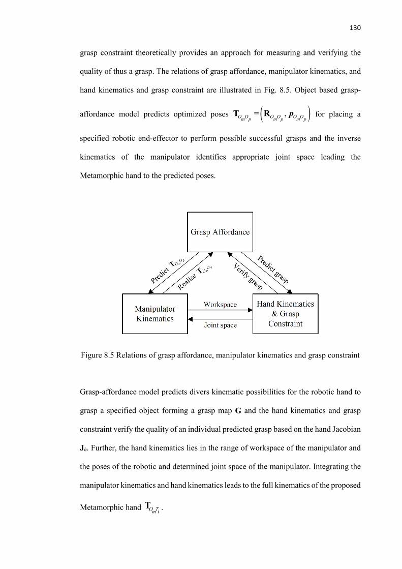
130
grasp constraint theoretically provides an approach for measuring and verifying the
quality of thus a grasp. The relations of grasp affordance, manipulator kinematics, and
hand kinematics and grasp constraint are illustrated in Fig. 8.5. Object based grasp-
affordance model predicts optimized poses ( )= ,O O O O O Om p m p m pT R p for placing a
specified robotic end-effector to perform possible successful grasps and the inverse
kinematics of the manipulator identifies appropriate joint space leading the
Metamorphic hand to the predicted poses.
Figure 8.5 Relations of grasp affordance, manipulator kinematics and grasp constraint
Grasp-affordance model predicts divers kinematic possibilities for the robotic hand to
grasp a specified object forming a grasp map G and the hand kinematics and grasp
constraint verify the quality of an individual predicted grasp based on the hand Jacobian
Jh. Further, the hand kinematics lies in the range of workspace of the manipulator and
the poses of the robotic and determined joint space of the manipulator. Integrating the
manipulator kinematics and hand kinematics leads to the full kinematics of the proposed
Metamorphic hand O Tm iT .
131
8.6 Conclusions
In this chapter, a new and economic mobile manipulator was designed and developed
by integrating a three-fingered Metamorphic hand and a customized 7-DOF arm-wrist
set into a mobile platform–Robotino 3.0. The structure of the proposed mobile
manipulator was presented and kinematics of the 7-DOF serial robot was investigated
based on the product-of-exponential method in Lie displacement group providing
background for leading the Metamorphic hand to the poses predicted with the grasp-
affordance model. Based on mechanism decomposition, kinematics of the three-
fingered Metamorphic robotic hand was subsequently implemented followed by the
construction of grasp map and grasp constraint of the hand laying a theoretical
foundation for measuring grasp quality for each individual grasp predicted by the grasp-
affordance model.
Furthermore, relations of the grasp-affordance model, manipulator kinematics and hand
kinematics with its associated grasp constraint were revealed and interpreted linking
kinematics in robotics with machine learning in computer science. The flexible mobile
manipulator presented in the chapter was developed for the application of clutter
clearing with special scenarios for toys clearing up in child’s room or in a nursery
environment.

132
Chapter 9 Geometric Topology with Product
Submanifolds on Metamorphic Hand Grasping
9.1 Introduction
When manipulating an object, a robotic hand system together with the object could be
modelled by an equivalent parallel mechanism[64,112]. Grasp constraints that being
applied to the object, performance analysis of the robotic hand, and further optimization
design of the robotic hand can be implemented by using such methodology. All these
modelling and analysis become more complicated immediately when doing
manipulation with the Metamorphic hand since a reconfigurable palm is integrated.
This chapter is to resolve the grasp constraints of an object manipulated by the
Metamorphic hand. To bridge the gap between the mechanism principle and
manipulation theory with the Metamorphic hand, an analytical method based on
product submanifolds in the scope of Lie group SE(3) is to be built and then to be
applied to the grasp constraint analysis. This chapter then established a method of Lie
group integrated topology diagram with reduction operations for analyzing complex
parallel mechanisms and manipulation performance with the Metamorphic hand.
133
9.2 Product Submanifolds and its Tangent Space
9.2.1 Product Submanifolds of SE(3)
This section is to retrieve several fundamental concepts in Lie groups and product
submanifolds from mathematical books[113,114], paving a way for using a product
submanifold based approach in the scope of Lie group to perform kinematics analysis
of the metamorphic hand with a reconfigurable palm.
A complex of the rigid motion group SE(3) can be defined as a subset of elements of
SE(3) and coined (3).C SE With the concept of the complex of SE(3), a submanifold
M of SE(3) can be regarded as a complex of SE(3) attached with the smooth group
operations and we coin it (3).M SE If the closure property is satisfied for M, a
subgroup S of SE(3) can be obtained and written as (3).S SE Alternatively, a
subgroup of SE(3) can be directly obtained from a complex of SE(3) in the case the
group axioms are fulfilled for the complex. The above relationship among the complex,
submanifold, and subgroup of SE(3) is described in the following three definitions and
is illustrated by the following commutative diagram in Fig. 9.1.
Definition 1. A complex of the rigid motion group SE(3) can be defined as a subset of
elements of SE(3) and coined (3).C SE
Definition 2. A submanifold of SE(3) is a complex of SE(3) attached with the smooth
group operations and designated as (3).M SE
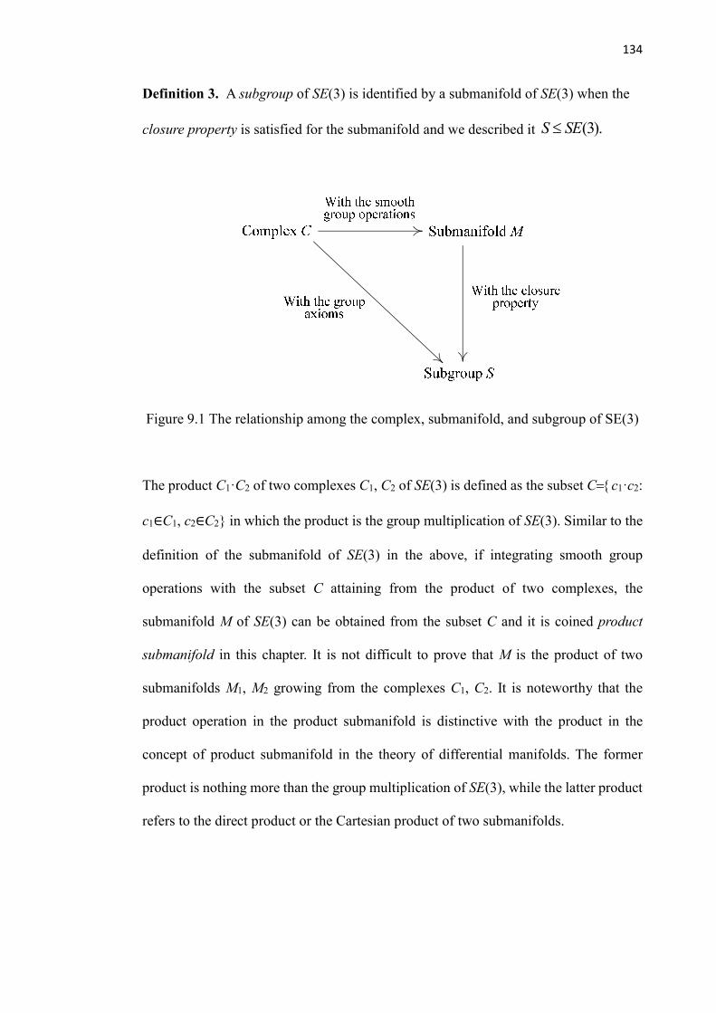
134
Definition 3. A subgroup of SE(3) is identified by a submanifold of SE(3) when the
closure property is satisfied for the submanifold and we described it (3).S SE
Figure 9.1 The relationship among the complex, submanifold, and subgroup of SE(3)
The product C1·C2 of two complexes C1, C2 of SE(3) is defined as the subset C=c1·c2:
c1∈C1, c2∈C2 in which the product is the group multiplication of SE(3). Similar to the
definition of the submanifold of SE(3) in the above, if integrating smooth group
operations with the subset C attaining from the product of two complexes, the
submanifold M of SE(3) can be obtained from the subset C and it is coined product
submanifold in this chapter. It is not difficult to prove that M is the product of two
submanifolds M1, M2 growing from the complexes C1, C2. It is noteworthy that the
product operation in the product submanifold is distinctive with the product in the
concept of product submanifold in the theory of differential manifolds. The former
product is nothing more than the group multiplication of SE(3), while the latter product
refers to the direct product or the Cartesian product of two submanifolds.

135
Definition 4. The product C1·C2 of two complexes C1, C2of SE(3) is defined as the
subset C=c1·c2: c1∈C1, c2∈C2, in which the product is the group multiplication of
SE(3).
Definition 5. If integrating smooth group operations with the subset C attaining from
the product of two complexes, the submanifold M of SE(3) can be obtained from the
subset C and, giving the product submanifold of submanifolds M1, M2 in which the two
submanifolds grow from the complexes C1, C2. It is described as M=M1·M2.
If more strictly, let the two complexes C1, C2 fulfil the group axioms, then two
subgroups S1, S2 are given. The product of subgroups S1, S2 of SE(3) does not
necessarily give another subgroup unless the closure property is satisfied for the
resultant subset of the product, but usually gives a product submanifold according to
the above definitions. In the same manner, we can derive the product of three or more
submanifolds or subgroups to generate a product submanifold of SE(3).
In kinematics, the product submanifold is, in fact, a mathematical representation of the
well-known kinematic bond put forward by Hervé [115].
9.2.2 Tangent Spaces of Product Submanifolds
In certain instances, the tangent space of a product submanifold plays an essential role
in mechanism analysis. From the differential geometry, the tangent space of a product
submanifold is equivalent to the product of the tangent spaces of the submanifolds[114].
Let M1, M2, …, Mn be a sequence of differential manifolds of dimension d1, d2, …, dn
respectively, a product submanifold M of dimension (d1 + d2 + … +dn) can be obtained
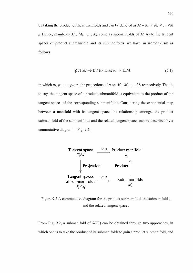
136
by taking the product of these manifolds and can be denoted as M = M1 × M2 × … ×M
n. Hence, manifolds M1, M2, … , Mn come as submanifolds of M. As to the tangent
spaces of product submanifold and its submanifolds, we have an isomorphism as
follows
1 21 2:T T T Tp np p pnM M M M ´ ´ ´ (9.1)
in which p1, p2, … , pn are the projections of p on M1, M2, …, Mn respectively. That is
to say, the tangent space of a product submanifold is equivalent to the product of the
tangent spaces of the corresponding submanifolds. Considering the exponential map
between a manifold with its tangent space, the relationship amongst the product
submanifold of the submanifolds and the related tangent spaces can be described by a
commutative diagram in Fig. 9.2.
Figure 9.2 A commutative diagram for the product submanifold, the submanifolds,
and the related tangent spaces
From Fig. 9.2, a submanifold of SE(3) can be obtained through two approaches, in
which one is to take the product of its submanifolds to gain a product submanifold, and
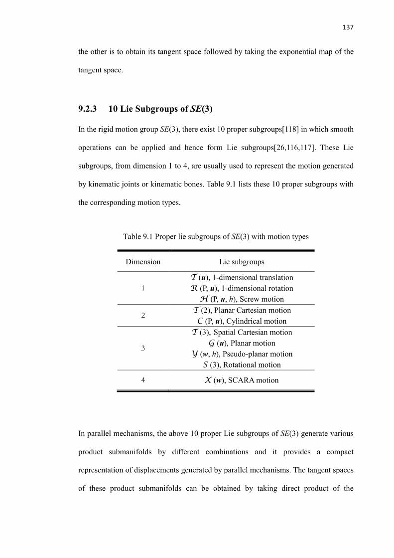
137
the other is to obtain its tangent space followed by taking the exponential map of the
tangent space.
9.2.3 10 Lie Subgroups of SE(3)
In the rigid motion group SE(3), there exist 10 proper subgroups[118] in which smooth
operations can be applied and hence form Lie subgroups[26,116,117]. These Lie
subgroups, from dimension 1 to 4, are usually used to represent the motion generated
by kinematic joints or kinematic bones. Table 9.1 lists these 10 proper subgroups with
the corresponding motion types.
Table 9.1 Proper lie subgroups of SE(3) with motion types
Dimension Lie subgroups
1
T (u), 1-dimensional translation
R (P, u), 1-dimensional rotation
H (P, u, h), Screw motion
2 T (2), Planar Cartesian motion
C (P, u), Cylindrical motion
3
T (3), Spatial Cartesian motion
G (u), Planar motion
Y (w, h), Pseudo-planar motion
S (3), Rotational motion
4 X (w), SCARA motion
In parallel mechanisms, the above 10 proper Lie subgroups of SE(3) generate various
product submanifolds by different combinations and it provides a compact
representation of displacements generated by parallel mechanisms. The tangent spaces
of these product submanifolds can be obtained by taking direct product of the
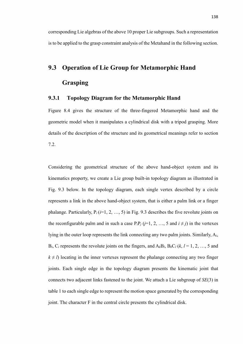
138
corresponding Lie algebras of the above 10 proper Lie subgroups. Such a representation
is to be applied to the grasp constraint analysis of the Metahand in the following section.
9.3 Operation of Lie Group for Metamorphic Hand
Grasping
9.3.1 Topology Diagram for the Metamorphic Hand
Figure 8.4 gives the structure of the three-fingered Metamorphic hand and the
geometric model when it manipulates a cylindrical disk with a tripod grasping. More
details of the description of the structure and its geometrical meanings refer to section
7.2.
Considering the geometrical structure of the above hand-object system and its
kinematics property, we create a Lie group built-in topology diagram as illustrated in
Fig. 9.3 below. In the topology diagram, each single vertex described by a circle
represents a link in the above hand-object system, that is either a palm link or a finger
phalange. Particularly, Pi (i=1, 2, …, 5) in Fig. 9.3 describes the five revolute joints on
the reconfigurable palm and in such a case PiPj (j=1, 2, …, 5 and i ≠ j) in the vertexes
lying in the outer loop represents the link connecting any two palm joints. Similarly, Ai,
Bi, Ci represents the revolute joints on the fingers, and AkBl, BkCl (k, l = 1, 2, …, 5 and
k ≠ l) locating in the inner vertexes represent the phalange connecting any two finger
joints. Each single edge in the topology diagram presents the kinematic joint that
connects two adjacent links fastened to the joint. We attach a Lie subgroup of SE(3) in
table 1 to each single edge to represent the motion space generated by the corresponding
joint. The character F in the central circle presents the cylindrical disk.

139
Figure 9.3 Lie group built-in topology diagram for the hand-object system with a
reconfigurable base
9.3.2 Lie Group Operations on Hand-Object Model
Such a representation of the topology benefits the modelling and analysis of the hand-
object system, especially the case that the robotic hand has a reconfigurable palm. It
makes the operations much easier to be done and provides a compact representation of
the operations, such as merging two adjacent edges or a series of connected edges,
deducting the motions using equivalent product submanifolds. For example, in Fig. 9.3,
if merging all the Lie subgroups from vertex P5P1 to F, the operation can be
implemented by considering definition 5 to take the product of several Lie subgroups
and the result can be obtained as
( ) ( ) ( ) 1 1 11 1 12 1A , B , C= x xM R R S (9.2)
.

140
To calculate the displacement representation of vertex F with respect to the base P5P1,
an iterative algorithm to deduct the above topology diagram is to be carried out by
applying the following two operations:
1. Compute the intersection of product submanifolds of two adjacent fingers.
2. Compute the intersection of product submanifolds on outer edges of the diagram
with restricted-displacement manifolds of the two related fingers.
From Fig. 9.3, the product submanifold for finger 2 and 3 can be presented respectively
as,
( ) ( ) ( ) 2 2 21 2 22 2A , B , C= x xM R R S (9.3)
( ) ( ) ( ) 3 3 31 3 32 3A , B , C= x xM R R S (9.4)
Two product submanifolds can be substituted by each other if they generate the same
Lie subgroup in table 1 or they are equivalent under group conjugation. Based on this
proposition, when joint P3 between fingers 2 and 3 are released and the other joints on
the metamorphic palm are locked, the above first operation which resolves the
intersection of product submanifolds of the two adjacent fingers can be achieved as
below
( ) ( ) 2 3 0 0P = yM M T S (9.5)
The above result represents the displacement submanifold of the platform under the
particular geometrical condition when only joint P3 on the palm is released.
Further, the above second operation can be applied as follows
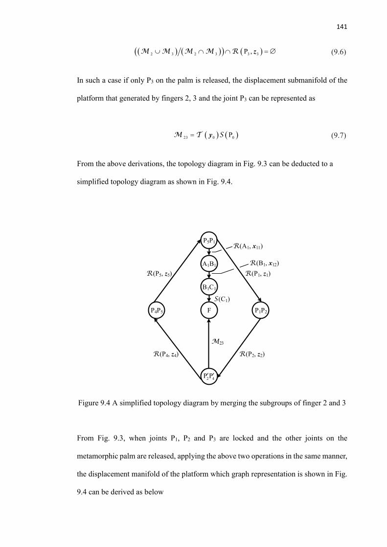
141
( ) ( )( ) ( ) 2 3 2 3 3 3P , = zM M M M R (9.6)
In such a case if only P3 on the palm is released, the displacement submanifold of the
platform that generated by fingers 2, 3 and the joint P3 can be represented as
( ) ( ) 23 0 0P= yM T S (9.7)
From the above derivations, the topology diagram in Fig. 9.3 can be deducted to a
simplified topology diagram as shown in Fig. 9.4.
Figure 9.4 A simplified topology diagram by merging the subgroups of finger 2 and 3
From Fig. 9.3, when joints P1, P2 and P3 are locked and the other joints on the
metamorphic palm are released, applying the above two operations in the same manner,
the displacement manifold of the platform which graph representation is shown in Fig.
9.4 can be derived as below
F
B1C1
A1B1
P5P1
P1P2P4P5
S (C1)
2 4P P
R (A1, x11)
R (B1, x12)
R (P1, z1)
R (P2, z2)R (P4, z4)
R (P5, z5)
M23
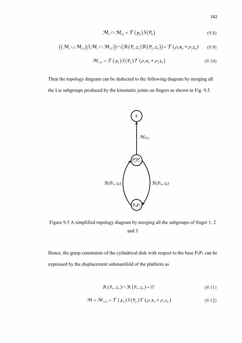
142
( ) ( ) 1 23 0 0P = yM M T S (9.8)
( ) ( )( ) ( ) ( )( ) ( ) 1 23 1 23 1 1 2 2 1 0 2 0P , P , =z z x + zM M M M R R T (9.9)
( ) ( ) ( ) 123 0 0 1 0 2 0P = y x + zM T S T (9.10)
Then the topology diagram can be deducted to the following diagram by merging all
the Lie subgroups produced by the kinematic joints on fingers as shown in Fig. 9.5.
Figure 9.5 A simplified topology diagram by merging all the subgroups of finger 1, 2
and 3
Hence, the grasp constraints of the cylindrical disk with respect to the base P5P1 can be
expressed by the displacement submanifold of the platform as
( ) ( )4 4 5 5P , P , = z zR R (9.11)
( ) ( ) ( ) 123 0 0 1 0 2 0P = = y x + zM M T S T (9.12)
F
4 5P P
R (P4, z4)R (P5, z5)
M123
P4P5
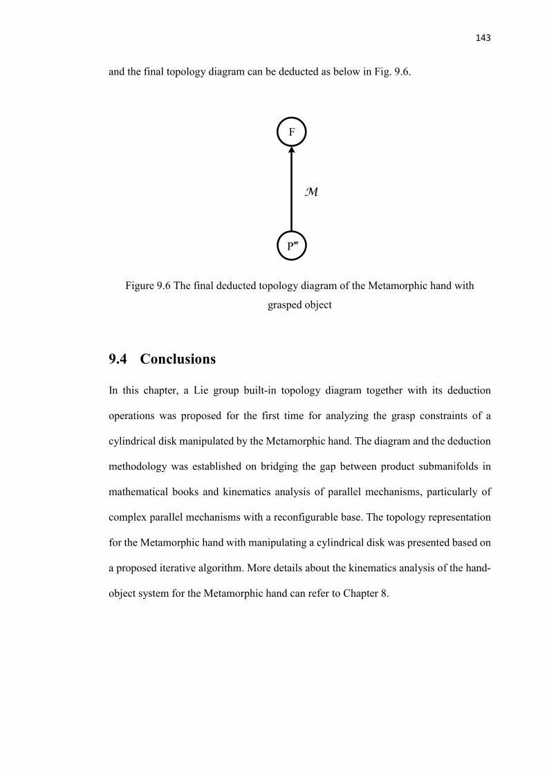
143
and the final topology diagram can be deducted as below in Fig. 9.6.
Figure 9.6 The final deducted topology diagram of the Metamorphic hand with
grasped object
9.4 Conclusions
In this chapter, a Lie group built-in topology diagram together with its deduction
operations was proposed for the first time for analyzing the grasp constraints of a
cylindrical disk manipulated by the Metamorphic hand. The diagram and the deduction
methodology was established on bridging the gap between product submanifolds in
mathematical books and kinematics analysis of parallel mechanisms, particularly of
complex parallel mechanisms with a reconfigurable base. The topology representation
for the Metamorphic hand with manipulating a cylindrical disk was presented based on
a proposed iterative algorithm. More details about the kinematics analysis of the hand-
object system for the Metamorphic hand can refer to Chapter 8.
F
M
P
144
Chapter 10 Geometry Variation Entailed
Metamorphic Hand Benchmarking and
Anthropomorphism Index
10.1 Introduction
The mechanical system of a robotic hand closely relates to its behaviours in grasping
and manipulation scenarios. The structure of a robotic hand consists of the architecture
of the palm and the arrangement of fingers. Instead of an inflexible palm, the
Metamorphic hand adopts a reconfigurable linkage mechanism as the palm with four
fingers attached on it. Hence the motion of fingers depends on the palm geometry
variation that awards fingers the additional capability to move in space in such a way
to enhance the performance in comparison to the conventional rigid-palm robotic hands.
This chapter proposes a new evaluation method based on the transverse metacarpal arch
to assess the palmar shape modulation of the Metamorphic hand. This method
investigates the palmar motion during the robot hand grasping. It is hypothesized that
the value of the arch indicates the closeness of the relative position of fingers. The
posture of the Metamorphic hand is related to both the kinematic transverse arch and
the rotation of the thumb base, which is different from human hands whose posture
changes are dominated by the palmar motion. The functional workspace is proposed as
145
an indicator to evaluate the precision grasp of the Metamorphic hand and demonstrate
the impact of the palm arch on grasp performance.
Gaussian Process Latent Variable Model[119] (GPLVM) is applied to evaluating the
four-fingered Metamorphic hand, and comparing its result to other robotic hands and
grippers with rigid palms. The area of hand workspace projected by GPLVM illustrates
its dexterity, namely the larger size of the projected area, the more dexterous of the
evaluated hand. The Metamorphic hand is evaluated in this way, and the result is
analysed in the light of various sampling sizes of actuated joints and configurations of
the palms.
10.2 Kinematic Transverse Arch of the Metamorphic Palm
10.2.1 The Kinematic Transverse Arch of Human Hands
The metamorphic palm is comprised of a five-bar spherical metamorphic mechanism.
The angular displacement of the closed-loop links is a way to mimic human palm
changes but its influence is not straight forward. In order to assess the change
objectively, we introduce a new description method called kinematic transverse arch to
evaluate the palmar shape modulations.
Anatomically, the human palm is described as two transverse metacarpal arches and
five longitudinal metacarpal arches shown in Fig.10.1(a) [120]. The palm arches
encompass a hollow cavity that changes its shape during pre-shaping and grasping
according to the geometry of the object. Sangole and Levin [121] gave a new
formulation about the transverse metacarpal arch called kinematic transverse arch when
studying the biomechanics of human palms. More specifically, the kinematic transverse
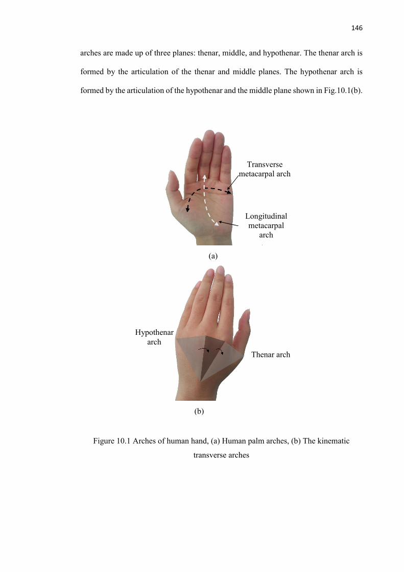
146
arches are made up of three planes: thenar, middle, and hypothenar. The thenar arch is
formed by the articulation of the thenar and middle planes. The hypothenar arch is
formed by the articulation of the hypothenar and the middle plane shown in Fig.10.1(b).
Figure 10.1 Arches of human hand, (a) Human palm arches, (b) The kinematic
transverse arches
Thenar arch
Hypothenar arch
(a)
(b)
Transverse metacarpal arch
Longitudinal metacarpal
arch

147
10.2.2 Transverse Arch Inspired Palm Geometry Variation Analysis
The ideas of kinematic transverse arches are applied to the motion analysis of the
metamorphic palm, shown in Fig.10.2. The thenar and hypothenar arch angles are
computed and the contribution of each to the arch formation will be expressed as a
percentage of the total angle. The kinematic transverse arch shows the palmar shape
modulation intuitively, the larger the value of the arch, the closer the relative position
of the fingers, especially among the thumb, the index finger and the middle finger, on
where most crawling actions and delicate operations mainly depend.
Figure 10.2 The kinematic transverse arch of the metamorphic palm
As shown in Fig.10.2, point P1 to P5 are the intersections between five fingers and the
reconfigurable palm. n1, n2 and n3 are the normals of planes P1OP2, P2OP3 and P3OP5
which express the thenar, middle, and hypothenar planes respectively. The equations of
these planes can be written as
0: ( ) 0i - = n r r , (10.1)

148
where, 0r is the vector directing to a fixed point and r is an arbitrary vector in the plane,
iop is the position vector that locates the ith finger with respect to the fixed coordinate
frame { 0 0 0O x y z- } that can be acquired as,
0
0
ji j i
ji i is c
=
=
op R op
op (10.2)
Where j indicates the number of the link connected to the ith finger and 0jR is the
rotation matrix of jth link with respect to the fixed frame. Thus, n1 to n3 can be obtained
by following equations,
1 2 2 3 3 5
1 2 3
1 2 2 3 3 5
, ,´ ´ ´
= = =´ ´ ´
op op op op op opn n n
op op op op op op . (10.3)
The thenar arch and hypothenar arch labeled as ϕ1 and ϕ2 are computed as,
1 1 2 2 2 3cos( ), cos( )arc arc = =n n n n . (10.4)
10.2.3 The Palm Geometry Variation related Actuation Constraints
The Metamorphic hand, shown in Fig. 10.3, is made up of a foldable palm and four
actuated fingers, i.e. a four-DOF thumb, an index finger, a middle finger and a ring
finger with three-DOF respectively. The little finger is omitted for simplifying the
complexity of design and control as it is less important than other fingers in terms of
functionality. The reconfigurable palm consists of five links which connect to each
other to form a spherical five-bar linkage mechanism. In order to maximize the

149
rotatability of the spherical five-bar linkage, the angles of link 1 to link 5 are considered
as 1 20 = , 2 40 = , 3 70 = , 4 112 = and 5 113 = , which need to satisfy the
conditions 1 2 3 4 5 360 + + + + = and 1 2 5 3 4 + + = + , presented in [107].
A thumb is mounted to link 2 by a revolute joint, which is similar to the CMC joint of
human hands. An index finger is installed on link 3, and the middle finger and ring
finger are mounted at link 4. All the fingers have three phalanxes that are connected by
revolute joints in parallel and follow the same design. Different from fingers mounted
at a fix palm, the Metamorphic hand has the capability to provide the
adduction/abduction motions for fingers so as to expand their workspace and increase
dexterity. Further, the maximum radius of the spherical linkage palm is designed at
50mm in the light of the size of an adult’s hand.
Figure 10.3 The Metamorphic hand with a reconfigurable palm
150
10.2.4 Geometric Constraints of the Metamorphic Palm
From the perspective of mechanism, the Metamorphic hand can be regarded as a hybrid
mechanism consisting of a closed-chain palm and four open-chain fingers. The
kinematics of the reconfigurable palm and fingers can be analyzed individually and then
combined for the whole hand kinematics.
The kinematics of the Metamorphic palm was well presented in [61]. In the reference,
joints A and E are treated as active joints of the palm, and joints B, C and D are passive
joints whose motion depends on the input of joints A and E. In order to identify the
geometric constraints of this reconfigurable palm, we use the same notions and
coordinate frames set up in reference [61].
When assigning the value of angle 5 , the spherical five-bar linkage mechanism
degenerates to a spherical four-bar linkage mechanism. At that time, rotating link 1 will
make the spherical four-bar linkage mechanism reach its limited positions when point
B, C and D are in the same plane, which is given by,
D B C( ) 0 ´ =P P P , (10.5)
B D C( ) 0 ´ =P P P . (10.6)
151
The mechanism has two limited positions as the link 1 can rotate on both sides with
respect to link 2. Thus, the value of θ5 decides the range of θ1, the relation between the
two angles can be obtained as,
T1cosB A =P P , (10.7)
T2 3cos( )B D = +P P , (10.8)
T 1B B =P P . (10.9)
Substituting PB and PD in [61] into Eq. (10.8) and solving the latter gives the two
limiting value of angle θ1 as
'
l 2 2arctan( ) arccos( )
Y Z
X X Y
-=
+ (10.10)
where 4 5 5 1 1 4 5s c c s s c sX = + , 1 4 5s s sY = and
2 3 1 4 5 4 1 5 5c( ) c c c s c c sZ = + - + .
So the range of θ1 with a specified θ5 is,
l2 2 2 2arctan( ) arccos( ) arctan( ) arccos( )
Y Z Y Z
X XX Y X Y
- -- +
+ + (10.11)
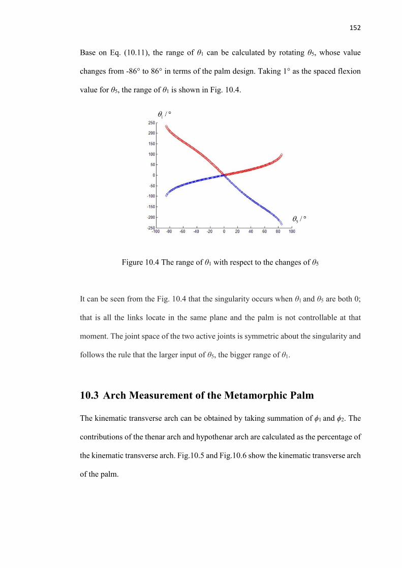
152
Base on Eq. (10.11), the range of θ1 can be calculated by rotating θ5, whose value
changes from -86° to 86° in terms of the palm design. Taking 1° as the spaced flexion
value for θ5, the range of θ1 is shown in Fig. 10.4.
Figure 10.4 The range of θ1 with respect to the changes of θ5
It can be seen from the Fig. 10.4 that the singularity occurs when θ1 and θ5 are both 0;
that is all the links locate in the same plane and the palm is not controllable at that
moment. The joint space of the two active joints is symmetric about the singularity and
follows the rule that the larger input of θ5, the bigger range of θ1.
10.3 Arch Measurement of the Metamorphic Palm
The kinematic transverse arch can be obtained by taking summation of ϕ1 and ϕ2. The
contributions of the thenar arch and hypothenar arch are calculated as the percentage of
the kinematic transverse arch. Fig.10.5 and Fig.10.6 show the kinematic transverse arch
of the palm.
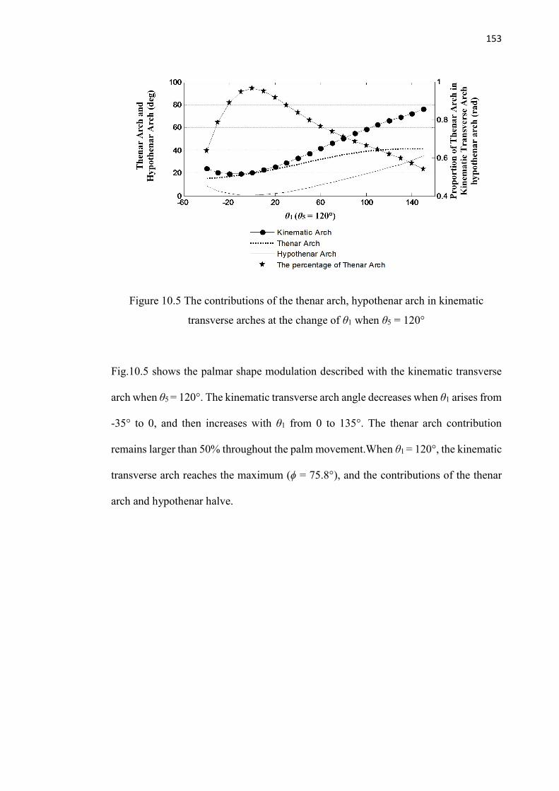
153
Figure 10.5 The contributions of the thenar arch, hypothenar arch in kinematic
transverse arches at the change of θ1 when θ5 = 120°
Fig.10.5 shows the palmar shape modulation described with the kinematic transverse
arch when θ5 = 120°. The kinematic transverse arch angle decreases when θ1 arises from
-35° to 0, and then increases with θ1 from 0 to 135°. The thenar arch contribution
remains larger than 50% throughout the palm movement.When θ1 = 120°, the kinematic
transverse arch reaches the maximum (ϕ = 75.8°), and the contributions of the thenar
arch and hypothenar halve.
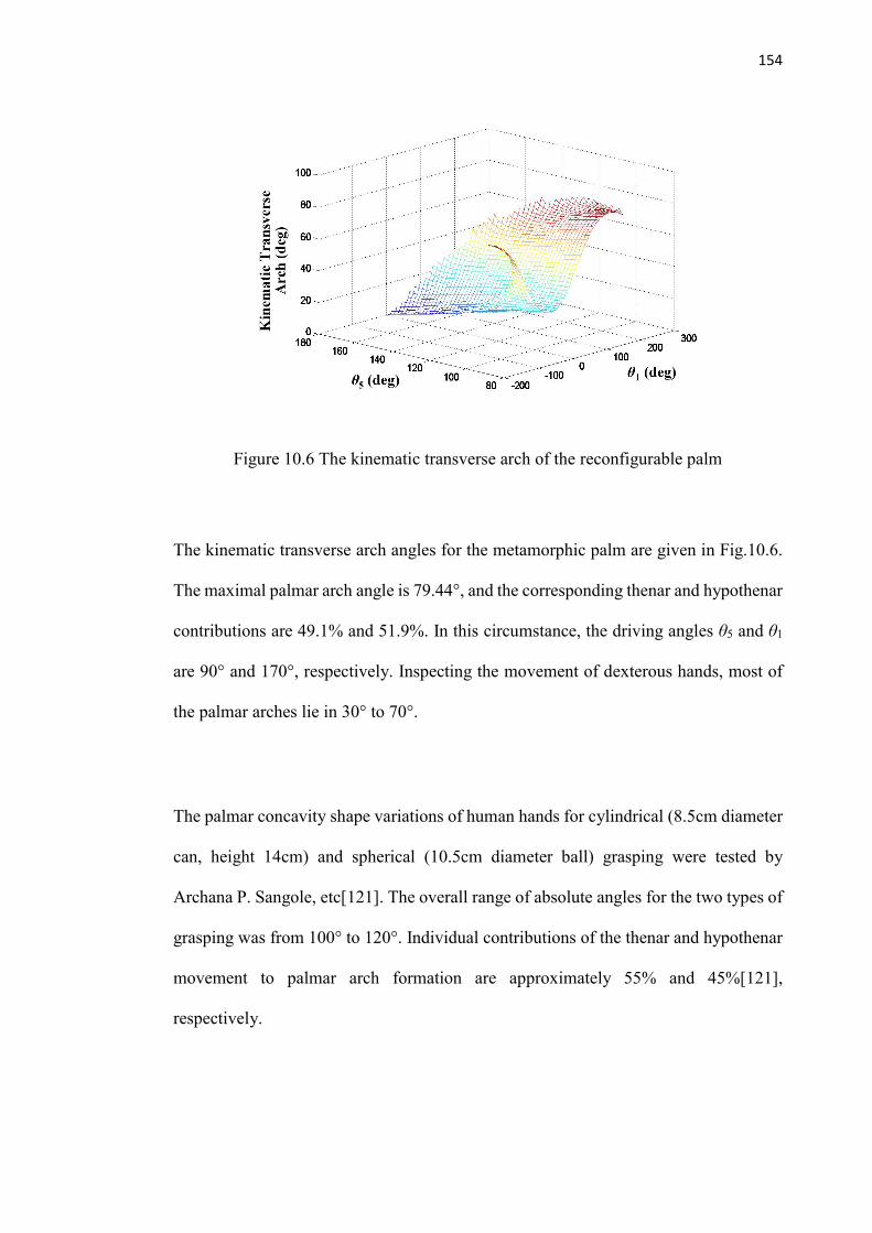
154
Figure 10.6 The kinematic transverse arch of the reconfigurable palm
The kinematic transverse arch angles for the metamorphic palm are given in Fig.10.6.
The maximal palmar arch angle is 79.44°, and the corresponding thenar and hypothenar
contributions are 49.1% and 51.9%. In this circumstance, the driving angles θ5 and θ1
are 90° and 170°, respectively. Inspecting the movement of dexterous hands, most of
the palmar arches lie in 30° to 70°.
The palmar concavity shape variations of human hands for cylindrical (8.5cm diameter
can, height 14cm) and spherical (10.5cm diameter ball) grasping were tested by
Archana P. Sangole, etc[121]. The overall range of absolute angles for the two types of
grasping was from 100° to 120°. Individual contributions of the thenar and hypothenar
movement to palmar arch formation are approximately 55% and 45%[121],
respectively.
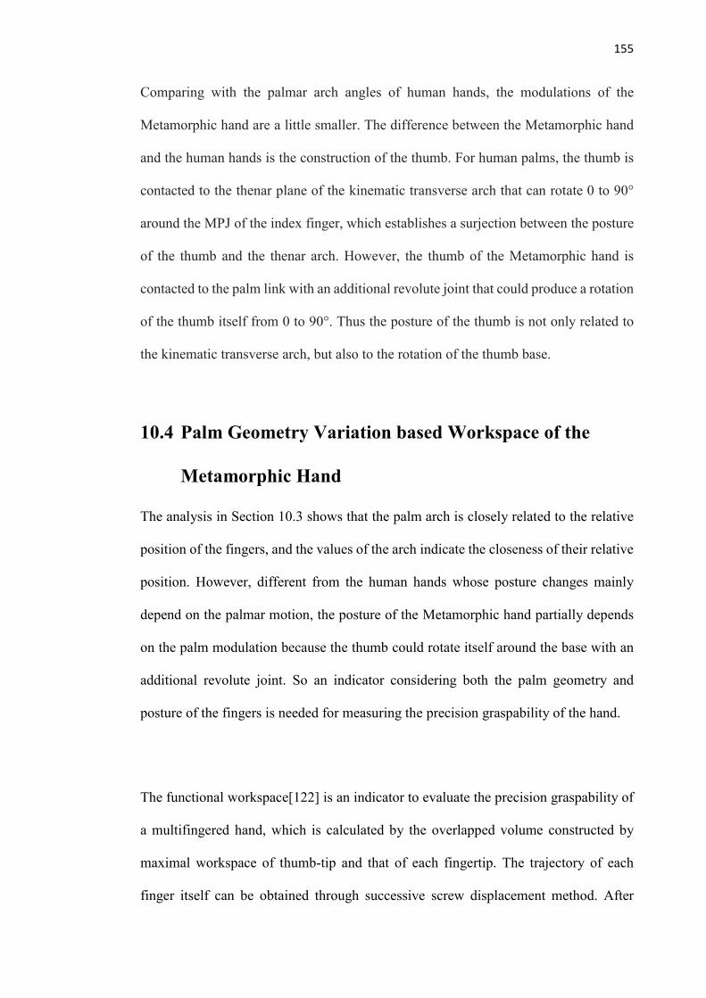
155
Comparing with the palmar arch angles of human hands, the modulations of the
Metamorphic hand are a little smaller. The difference between the Metamorphic hand
and the human hands is the construction of the thumb. For human palms, the thumb is
contacted to the thenar plane of the kinematic transverse arch that can rotate 0 to 90°
around the MPJ of the index finger, which establishes a surjection between the posture
of the thumb and the thenar arch. However, the thumb of the Metamorphic hand is
contacted to the palm link with an additional revolute joint that could produce a rotation
of the thumb itself from 0 to 90°. Thus the posture of the thumb is not only related to
the kinematic transverse arch, but also to the rotation of the thumb base.
10.4 Palm Geometry Variation based Workspace of the
Metamorphic Hand
The analysis in Section 10.3 shows that the palm arch is closely related to the relative
position of the fingers, and the values of the arch indicate the closeness of their relative
position. However, different from the human hands whose posture changes mainly
depend on the palmar motion, the posture of the Metamorphic hand partially depends
on the palm modulation because the thumb could rotate itself around the base with an
additional revolute joint. So an indicator considering both the palm geometry and
posture of the fingers is needed for measuring the precision graspability of the hand.
The functional workspace[122] is an indicator to evaluate the precision graspability of
a multifingered hand, which is calculated by the overlapped volume constructed by
maximal workspace of thumb-tip and that of each fingertip. The trajectory of each
finger itself can be obtained through successive screw displacement method. After
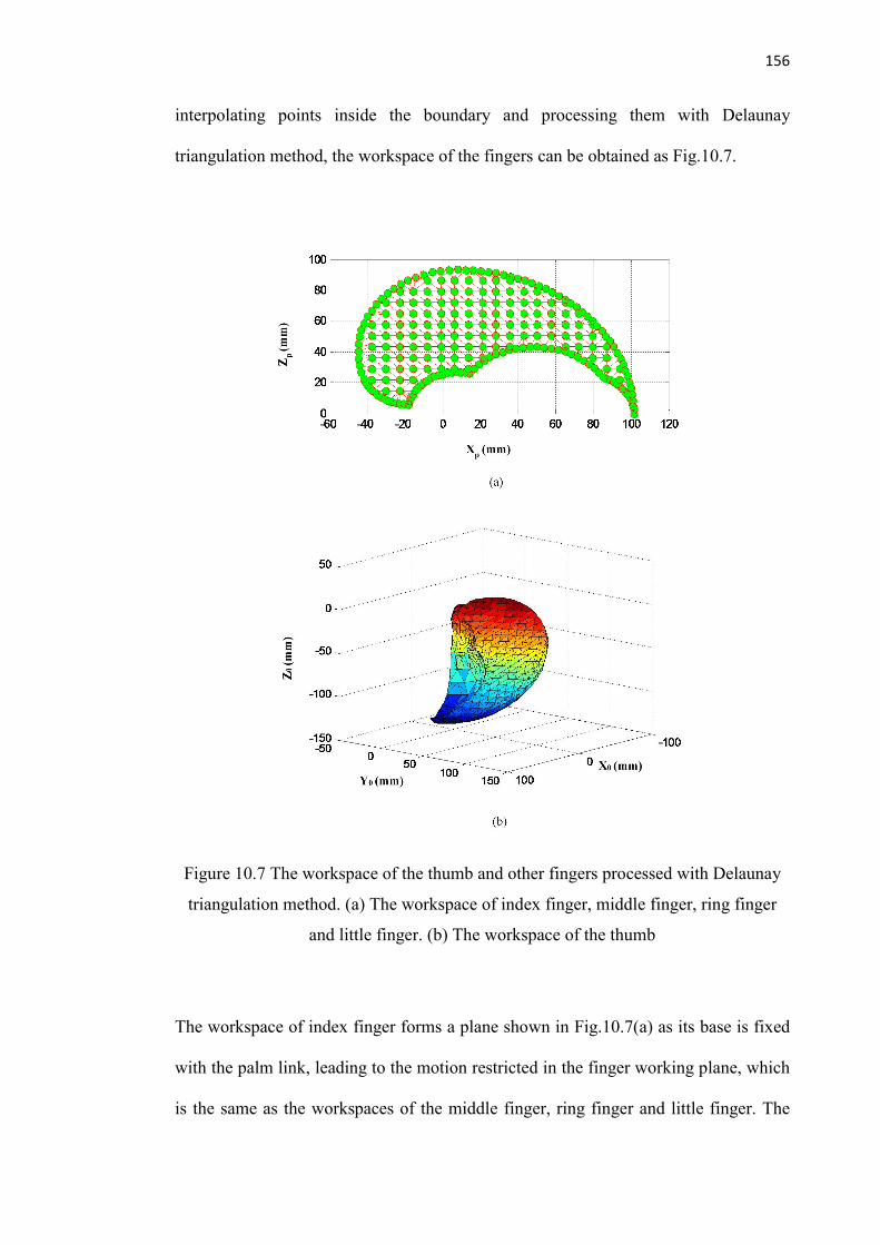
156
interpolating points inside the boundary and processing them with Delaunay
triangulation method, the workspace of the fingers can be obtained as Fig.10.7.
Figure 10.7 The workspace of the thumb and other fingers processed with Delaunay
triangulation method. (a) The workspace of index finger, middle finger, ring finger
and little finger. (b) The workspace of the thumb
The workspace of index finger forms a plane shown in Fig.10.7(a) as its base is fixed
with the palm link, leading to the motion restricted in the finger working plane, which
is the same as the workspaces of the middle finger, ring finger and little finger. The
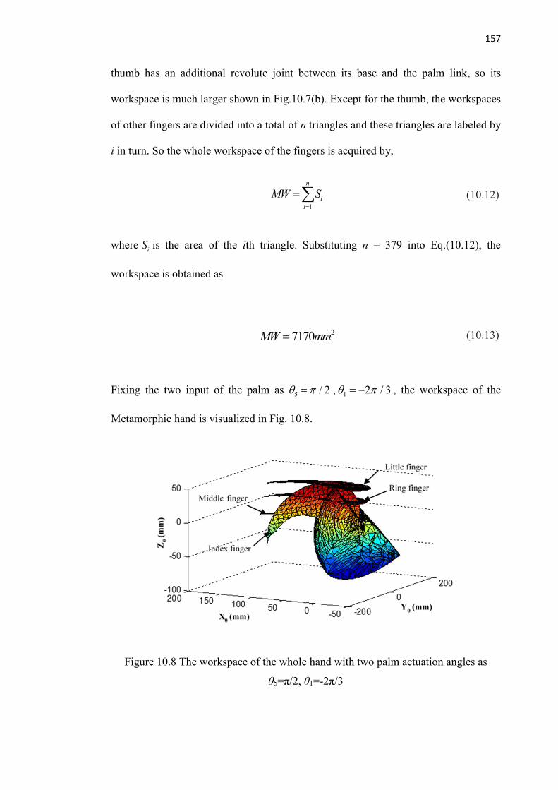
157
thumb has an additional revolute joint between its base and the palm link, so its
workspace is much larger shown in Fig.10.7(b). Except for the thumb, the workspaces
of other fingers are divided into a total of n triangles and these triangles are labeled by
i in turn. So the whole workspace of the fingers is acquired by,
1
n
ii
MW S=
= (10.12)
where iS is the area of the ith triangle. Substituting n = 379 into Eq.(10.12), the
workspace is obtained as
27170MW mm= (10.13)
Fixing the two input of the palm as 5 / 2 = , 1 2 / 3 = - , the workspace of the
Metamorphic hand is visualized in Fig. 10.8.
Figure 10.8 The workspace of the whole hand with two palm actuation angles as
θ5=π/2, θ1=-2π/3
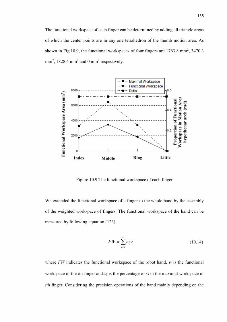
158
The functional workspace of each finger can be determined by adding all triangle areas
of which the center points are in any one tetrahedron of the thumb motion area. As
shown in Fig.10.9, the functional workspaces of four fingers are 1763.8 mm2, 3470.3
mm2, 1828.4 mm2 and 0 mm2 respectively.
Figure 10.9 The functional workspace of each finger
We extended the functional workspace of a finger to the whole hand by the assembly
of the weighted workspace of fingers. The functional workspace of the hand can be
measured by following equation [123],
2
k
i ii
FW ω v=
= (10.14)
where FW indicates the functional workspace of the robot hand, vi is the functional
workspace of the ith finger and i is the percentage of vi in the maximal workspace of
ith finger. Considering the precision operations of the hand mainly depending on the
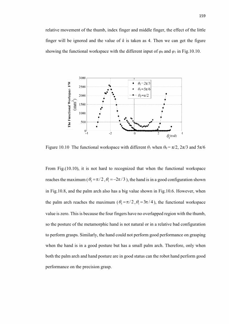
159
relative movement of the thumb, index finger and middle finger, the effect of the little
finger will be ignored and the value of k is taken as 4. Then we can get the figure
showing the functional workspace with the different input of φ0 and φ1 in Fig.10.10.
Figure 10.10 The functional workspace with different θ1 when θ0 = π/2, 2π/3 and 5π/6
From Fig.(10.10), it is not hard to recognized that when the functional workspace
reaches the maximum ( 5 = , 1 2 =- ), the hand is in a good configuration shown
in Fig.10.8, and the palm arch also has a big value shown in Fig.10.6. However, when
the palm arch reaches the maximum ( 5 = , 1 3 = ), the functional workspace
value is zero. This is because the four fingers have no overlapped region with the thumb,
so the posture of the metamorphic hand is not natural or in a relative bad configuration
to perform grasps. Similarly, the hand could not perform good performance on grasping
when the hand is in a good posture but has a small palm arch. Therefore, only when
both the palm arch and hand posture are in good status can the robot hand perform good
performance on the precision grasp.
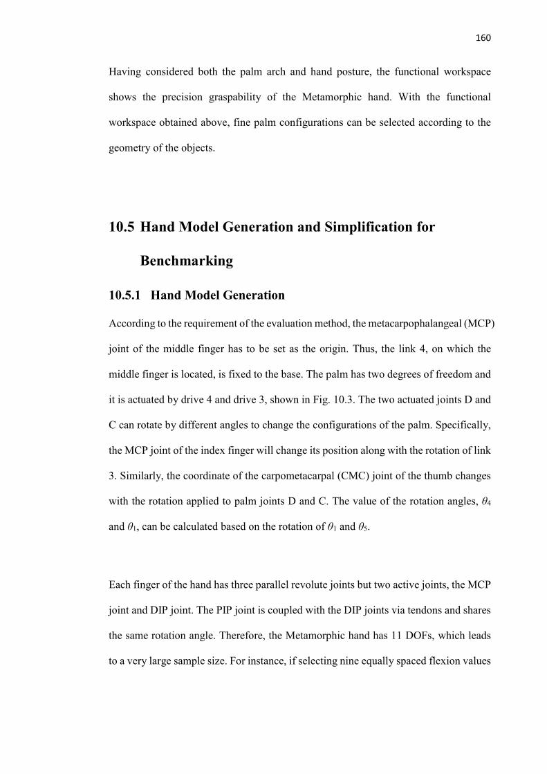
160
Having considered both the palm arch and hand posture, the functional workspace
shows the precision graspability of the Metamorphic hand. With the functional
workspace obtained above, fine palm configurations can be selected according to the
geometry of the objects.
10.5 Hand Model Generation and Simplification for
Benchmarking
10.5.1 Hand Model Generation
According to the requirement of the evaluation method, the metacarpophalangeal (MCP)
joint of the middle finger has to be set as the origin. Thus, the link 4, on which the
middle finger is located, is fixed to the base. The palm has two degrees of freedom and
it is actuated by drive 4 and drive 3, shown in Fig. 10.3. The two actuated joints D and
C can rotate by different angles to change the configurations of the palm. Specifically,
the MCP joint of the index finger will change its position along with the rotation of link
3. Similarly, the coordinate of the carpometacarpal (CMC) joint of the thumb changes
with the rotation applied to palm joints D and C. The value of the rotation angles, θ4
and θ1, can be calculated based on the rotation of θ1 and θ5.
Each finger of the hand has three parallel revolute joints but two active joints, the MCP
joint and DIP joint. The PIP joint is coupled with the DIP joints via tendons and shares
the same rotation angle. Therefore, the Metamorphic hand has 11 DOFs, which leads
to a very large sample size. For instance, if selecting nine equally spaced flexion values
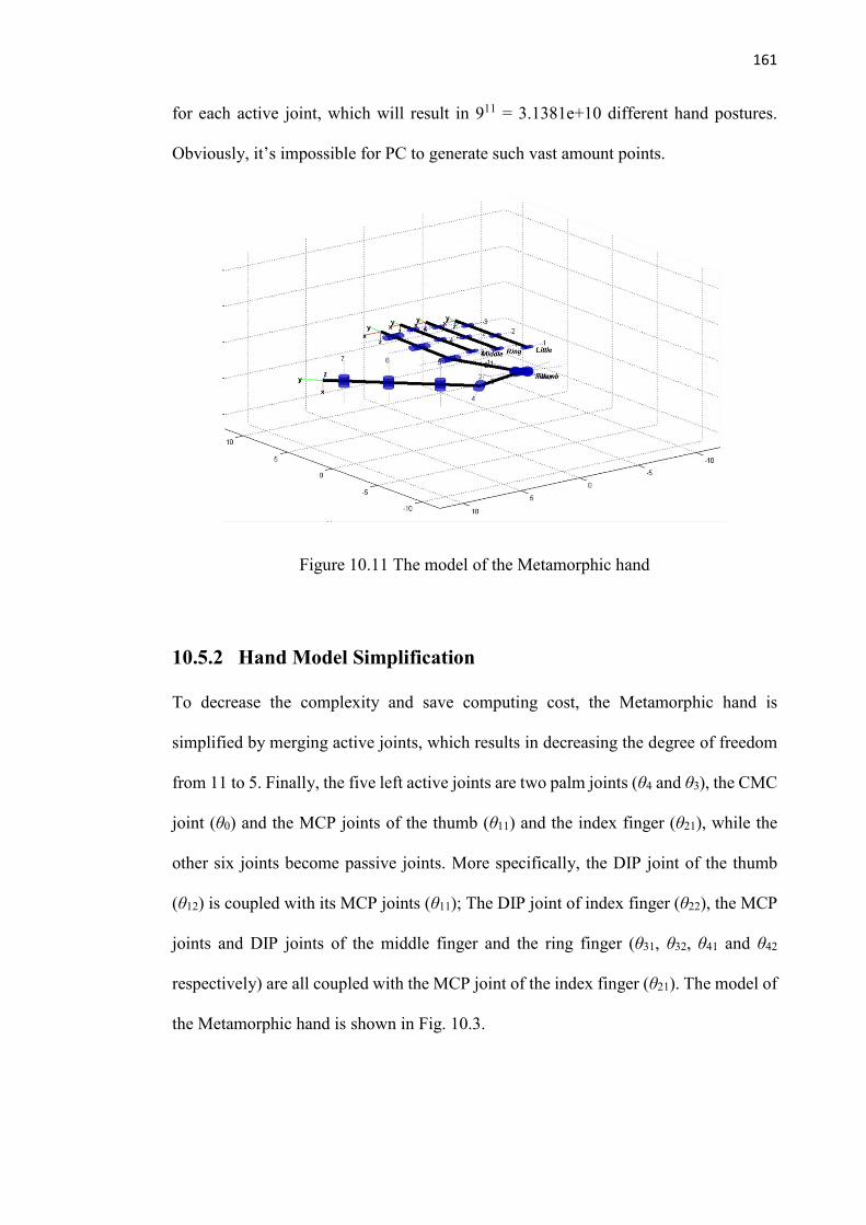
161
for each active joint, which will result in 911 = 3.1381e+10 different hand postures.
Obviously, it’s impossible for PC to generate such vast amount points.
Figure 10.11 The model of the Metamorphic hand
10.5.2 Hand Model Simplification
To decrease the complexity and save computing cost, the Metamorphic hand is
simplified by merging active joints, which results in decreasing the degree of freedom
from 11 to 5. Finally, the five left active joints are two palm joints (θ4 and θ3), the CMC
joint (θ0) and the MCP joints of the thumb (θ11) and the index finger (θ21), while the
other six joints become passive joints. More specifically, the DIP joint of the thumb
(θ12) is coupled with its MCP joints (θ11); The DIP joint of index finger (θ22), the MCP
joints and DIP joints of the middle finger and the ring finger (θ31, θ32, θ41 and θ42
respectively) are all coupled with the MCP joint of the index finger (θ21). The model of
the Metamorphic hand is shown in Fig. 10.3.
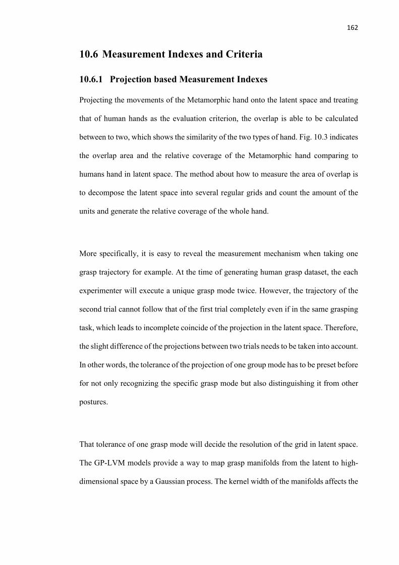
162
10.6 Measurement Indexes and Criteria
10.6.1 Projection based Measurement Indexes
Projecting the movements of the Metamorphic hand onto the latent space and treating
that of human hands as the evaluation criterion, the overlap is able to be calculated
between to two, which shows the similarity of the two types of hand. Fig. 10.3 indicates
the overlap area and the relative coverage of the Metamorphic hand comparing to
humans hand in latent space. The method about how to measure the area of overlap is
to decompose the latent space into several regular grids and count the amount of the
units and generate the relative coverage of the whole hand.
More specifically, it is easy to reveal the measurement mechanism when taking one
grasp trajectory for example. At the time of generating human grasp dataset, the each
experimenter will execute a unique grasp mode twice. However, the trajectory of the
second trial cannot follow that of the first trial completely even if in the same grasping
task, which leads to incomplete coincide of the projection in the latent space. Therefore,
the slight difference of the projections between two trials needs to be taken into account.
In other words, the tolerance of the projection of one group mode has to be preset before
for not only recognizing the specific grasp mode but also distinguishing it from other
postures.
That tolerance of one grasp mode will decide the resolution of the grid in latent space.
The GP-LVM models provide a way to map grasp manifolds from the latent to high-
dimensional space by a Gaussian process. The kernel width of the manifolds affects the

163
tolerance of one grasp, resulting in a different value of overlap area in the same set of
hands postures.
10.6.2 Evaluation of the Metamorphic Hand based on AI1
Depending on the simplification mentioned above, the Metamorphic hand can be driven
based on the reduced model. The strategy of how to select hand postures driven by five
positive joints, θ0, θ11, θ21, θ3 and θ4, is described as follows. The value of θ0, θ11, and
θ21 ranges from 0 to 80° with 9 equally spaced samples taken from that range, where
θ(1) = 0 is finger opened and θ(9) = 80° is finger closed. For the two palm joints, θ4 and
θ3, are assigned with 120 sets of value according to the geometric constraints of the
palm. Overall, it generates 120×93 = 87480 different hand postures.
After projecting those hand poses onto the latent space, The AI is 12.69%, shown in
Fig. 10.6 (a). Generally speaking, the value will be increased along with the extension
of sample size. Thus, the actual value of 11-DOF Metamorphic hand must be higher
than 12.69%.
10.6.3 The Improvement of AI with the Reconfigurable Palm
In order to indicate the affection of reconfigurable palm to AI, the properties of the
Metamorphic hand can be updated as the fixed palm, and the influence on the latent
space overlap can be analyzed. The angles of two palm joints are fastened at the initial
state. So the value of θ3 and θ4 is zero. Give the same range and value of θ0, θ11 and θ12
1 Anthropomorphism Index
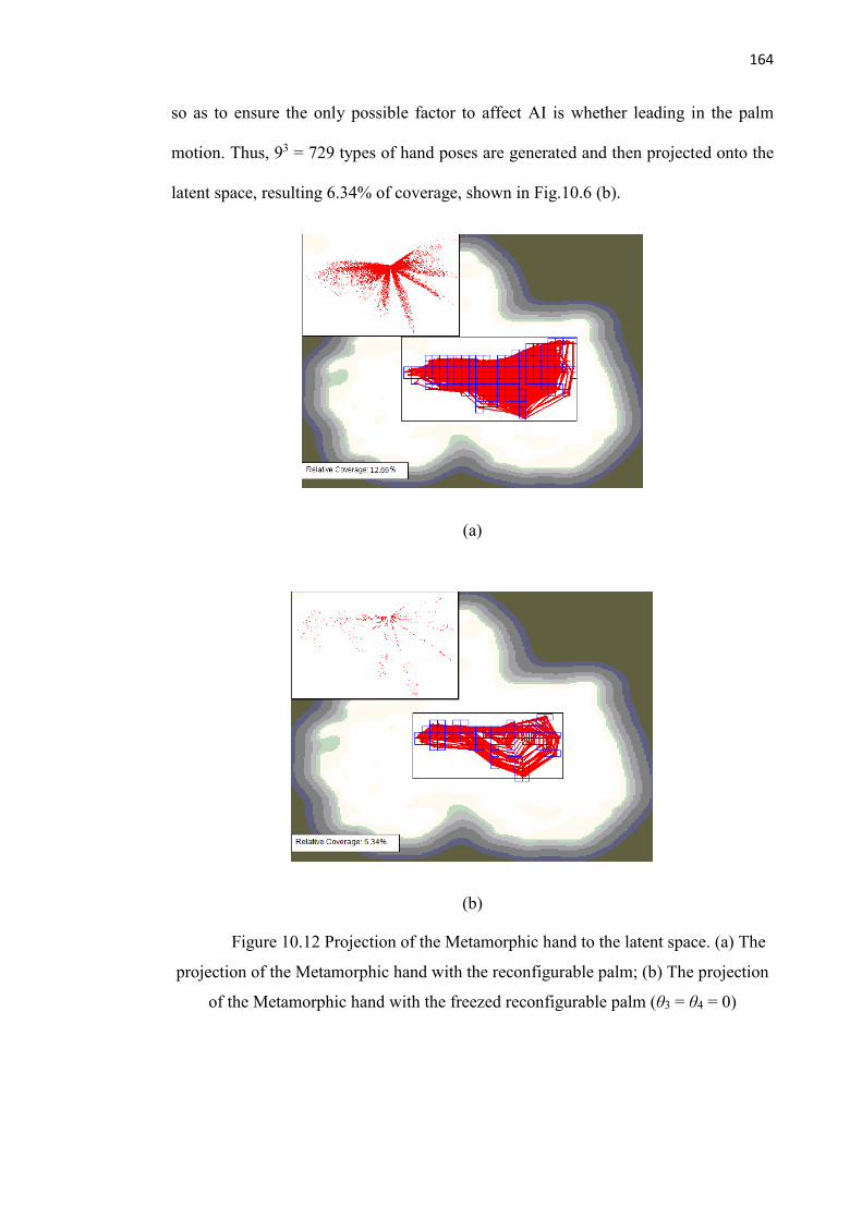
164
so as to ensure the only possible factor to affect AI is whether leading in the palm
motion. Thus, 93 = 729 types of hand poses are generated and then projected onto the
latent space, resulting 6.34% of coverage, shown in Fig.10.6 (b).
(a)
(b)
Figure 10.12 Projection of the Metamorphic hand to the latent space. (a) The
projection of the Metamorphic hand with the reconfigurable palm; (b) The projection
of the Metamorphic hand with the freezed reconfigurable palm (θ3 = θ4 = 0)
165
The AI corresponding to the Metamorphic hand with reconfigurable palm is twice as
that with the fixed palm. The comparison proves that the reconfigurable palm of the
Metamorphic hand improves the AI, as well as the graspability and dexterity.
10.7 Comparison of the Metamorphic Hand with Selected
Robotic hands
10.7.1 The Effect of Number of DODs
The AI of the Metamorphic hand (12.69%) is much higher that of SensorHand [124]
(0.25%), Michelangelo Hand [125] (2.8%) and FRH-4 Hand [126] (5.2%), illustrated
in Form 1. The reasons why the evaluation system generated the very low value of AI
of SensorHand and Michelangelo Hand mainly because they had few degree of
freedoms. For the SensorHand, it just has one DOF and three fingers, in which most of
the joints are rigid. Thus, there is no doubt that SensorHand produces such a low score
and its graspability is obviously poor. While mentioning the Michelangelo hand, it has
Two DOFs and five fingers. Although most of the joints are coupled, the value of AI is
much higher than that of SensorHand relatively. Similarly, it shows the same results
when comparing Michelangelo Hand to FRH-4 Hand and the Metamorphic hand.
These comparisons demonstrate that the number of DOFs is a critical factor affecting
the score of the evaluation. So increasing the number of DOFs and bringing in more
active joints can enhance the dexterity of the robotic hands.
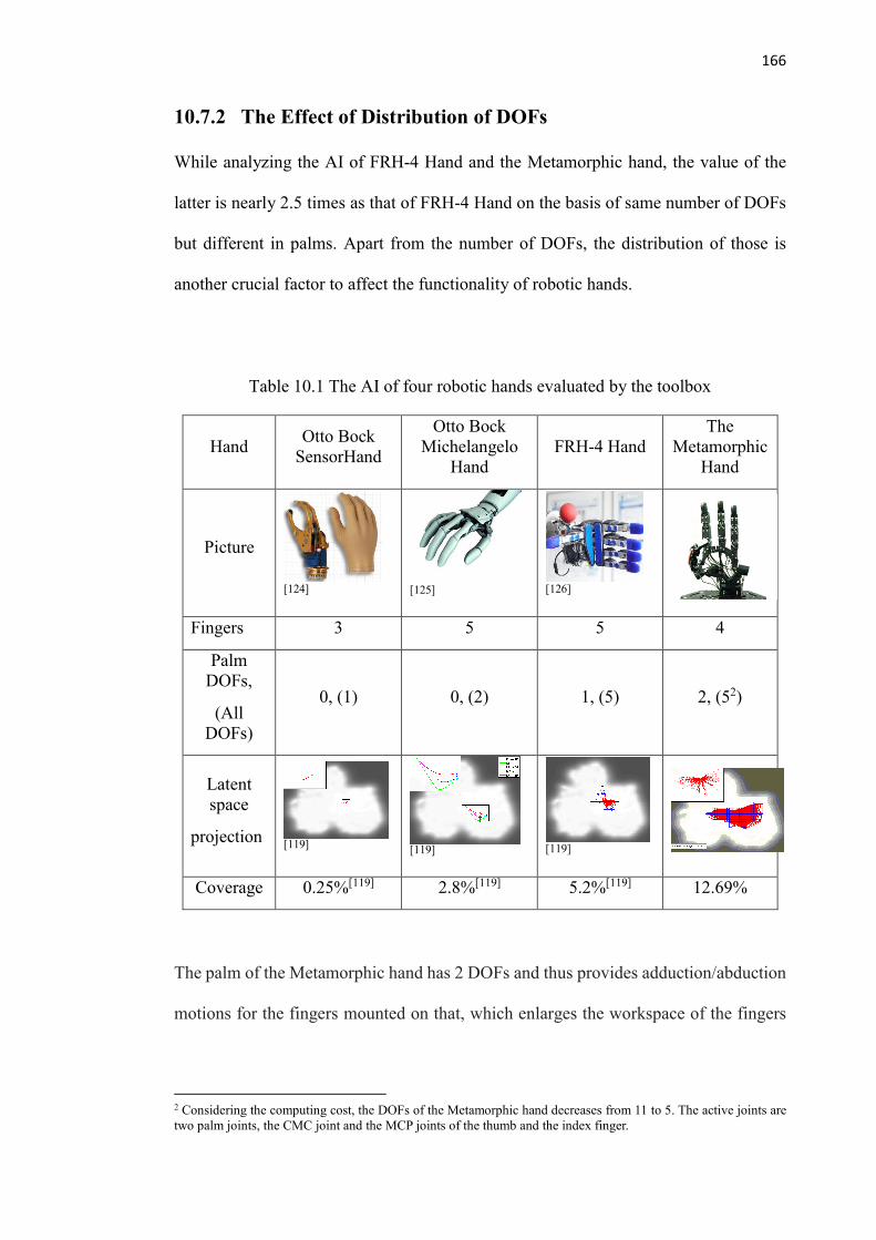
166
10.7.2 The Effect of Distribution of DOFs
While analyzing the AI of FRH-4 Hand and the Metamorphic hand, the value of the
latter is nearly 2.5 times as that of FRH-4 Hand on the basis of same number of DOFs
but different in palms. Apart from the number of DOFs, the distribution of those is
another crucial factor to affect the functionality of robotic hands.
Table 10.1 The AI of four robotic hands evaluated by the toolbox
Hand Otto Bock
SensorHand
Otto Bock Michelangelo
Hand FRH-4 Hand
The Metamorphic
Hand
Picture
[124] [125] [126]
Fingers 3 5 5 4
Palm DOFs,
(All DOFs)
0, (1) 0, (2) 1, (5) 2, (52)
Latent space
projection [119] [119] [119]
Coverage 0.25%[119] 2.8%[119] 5.2%[119] 12.69%
The palm of the Metamorphic hand has 2 DOFs and thus provides adduction/abduction
motions for the fingers mounted on that, which enlarges the workspace of the fingers
2 Considering the computing cost, the DOFs of the Metamorphic hand decreases from 11 to 5. The active joints are two palm joints, the CMC joint and the MCP joints of the thumb and the index finger.
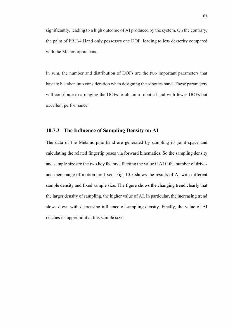
167
significantly, leading to a high outcome of AI produced by the system. On the contrary,
the palm of FRH-4 Hand only possesses one DOF, leading to less dexterity compared
with the Metamorphic hand.
In sum, the number and distribution of DOFs are the two important parameters that
have to be taken into consideration when designing the robotics hand. These parameters
will contribute to arranging the DOFs to obtain a robotic hand with fewer DOFs but
excellent performance.
10.7.3 The Influence of Sampling Density on AI
The data of the Metamorphic hand are generated by sampling its joint space and
calculating the related fingertip poses via forward kinematics. So the sampling density
and sample size are the two key factors affecting the value if AI if the number of drives
and their range of motion are fixed. Fig. 10.5 shows the results of AI with different
sample density and fixed sample size. The figure shows the changing trend clearly that
the larger density of sampling, the higher value of AI. In particular, the increasing trend
slows down with decreasing influence of sampling density. Finally, the value of AI
reaches its upper limit at this sample size.
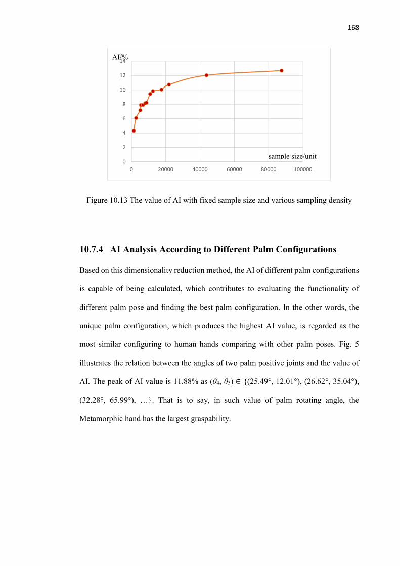
168
Figure 10.13 The value of AI with fixed sample size and various sampling density
10.7.4 AI Analysis According to Different Palm Configurations
Based on this dimensionality reduction method, the AI of different palm configurations
is capable of being calculated, which contributes to evaluating the functionality of
different palm pose and finding the best palm configuration. In the other words, the
unique palm configuration, which produces the highest AI value, is regarded as the
most similar configuring to human hands comparing with other palm poses. Fig. 5
illustrates the relation between the angles of two palm positive joints and the value of
AI. The peak of AI value is 11.88% as (θ4, θ3) {(25.49°, 12.01°), (26.62°, 35.04°),
(32.28°, 65.99°), …}. That is to say, in such value of palm rotating angle, the
Metamorphic hand has the largest graspability.
0
2
4
6
8
10
12
14
0 20000 40000 60000 80000 100000
sample size/unit
AI/%
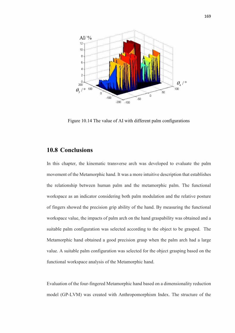
169
Figure 10.14 The value of AI with different palm configurations
10.8 Conclusions
In this chapter, the kinematic transverse arch was developed to evaluate the palm
movement of the Metamorphic hand. It was a more intuitive description that establishes
the relationship between human palm and the metamorphic palm. The functional
workspace as an indicator considering both palm modulation and the relative posture
of fingers showed the precision grip ability of the hand. By measuring the functional
workspace value, the impacts of palm arch on the hand graspability was obtained and a
suitable palm configuration was selected according to the object to be grasped. The
Metamorphic hand obtained a good precision grasp when the palm arch had a large
value. A suitable palm configuration was selected for the object grasping based on the
functional workspace analysis of the Metamorphic hand.
Evaluation of the four-fingered Metamorphic hand based on a dimensionality reduction
model (GP-LVM) was created with Anthropomorphism Index. The structure of the
170
Metamorphic hand was introduced which is regarded as a hybrid mechanism consisting
of a closed-chain palm and four open-chain fingers. The actuation constraints of palm
were reviewed through analysing the geometric constraints of the reconfigurable palm.
Simplification for the Metamorphic hand was explained in consideration of the
computation cost. Based on the reduced hand model, the Anthropomorphism Index of
the Metamorphic hand was calculated by 12.69%, which was much higher than that of
some selected robotic hands because of bringing in the palm variation. In addition, the
sample density and distribution of DOFs that affected the results significantly were
analysed for finding the most similar configuration to human hands. The Metamorphic
hand demonstrated good graspability adaptability and manipulability comparing to
other robotic hands with a fixed palm.

171
Chapter 11 Conclusions
11.1 General Conclusions
This thesis was dedicated to the study of the intrinsic connection between screw
coordinates from the perspective of geometry, and its derived Jacobian in contrast with
the derivative Jacobian, and their uses in velocity analysis and evaluation of the
Metamorphic hand. The general conclusions of the thesis is stated as follows,
Chapter 1 introduced the problems, aims and objectives of the thesis.
Chapter 2 presented the background and prior knowledge used in the following chapters,
specifically the line geometry, line coordinates, screw coordinates and its applications
in the analysis of first-order kinematics, state-of-the-art of parallel mechanisms and
dexterous hands and their latest development with the ideology of Metamorphosis
which led to the reconfigurable base-integrated parallel mechanism and the
Metamorphic hand.
Chapter 3 revealed the interconnection of screw coordinates from its original line
coordinates, namely ray coordinates and axis coordinates. From the geometrical
presentation of a line as a ray of two points, a triangle was constructed with its
projection on three coordinate planes making up the secondary part of ray coordinates.
Its counterpart, a reciprocal triangle was constructed for the first time by the plane
normals to give the geometrical representation of axis coordinates. In this way, the
geometrical meaning of axis coordinates was revealed with its primary part as the
172
vectors subtraction of the weighted plane normals and secondary part as their cross
product.
Chapter 4 was the follow-on study on the screw coordinates and revealed their intrinsic
connections from the perspective of geometry. The triangle derived from ray
coordinates and its counterpart, the reciprocal triangle derived from axis coordinates
were connected geometrically and algebraically, and then extended to conformability
and duality of ray coordinates and its reciprocal, axis coordinates. The correlation was
established with their correlated part ratios to relate the vector space to the dual vector
space where the ray coordinates and axis coordinates were constructed. At last, the
correlation operator that mapped the vector space to its dual vector was explained with
a conformability graph.
Chapter 5 investigated the geometrical meaning of a twist and its decomposition into a
rotation about an axis and a translation parallel to that axis. This chapter also presented
the compound of twists of a serial manipulator and its generation, the resultant twist,
geometrically and algebraically. Then the position vector of ISA of the resultant twist
was formulated by weighted position vectors of joint screws. Further, the screw based
Jacobian was proposed with the unit joint screws as its columns.
Chapter 6 was the further investigation based on chapter 5 and related the screw-based
Jacobian to the derivative method based Jacobian of the same manipulator. The relation
of a resultant twist and the end-effector velocity was formulated through an adjoint
transformation acting on the twist. This study was then pushed to explore the
reconciliation of Jacobians calculated by screw algebra and derivative method. Finally,

173
a planar 3R serial manipulator and a spatial serial manipulator examples varied this
adjoint transformation of two methods.
Chapter 7 proposed a novel parallel mechanism with a reconfigurable base inspired by
the manipulation of an object with a Metamorphic hand. The geometrical constraints of
the base were investigated, followed by the kinematics analysis of the parallel
mechanism. The forward and inverse kinematics solutions were calculated based on the
mechanism decomposition principle together with screw-based Jacobian, which
demonstrated the enlargement of the workspace of this reconfigurable base-integrated
parallel mechanism.
Chapter 8 proposed the design of a 7-DOF serial manipulator with a Metamorphic hand
attached at its distal end. The kinematics of the manipulator was investigated through a
product-of-exponential method in Lie group, followed by the analysis of grasping
constraints of the three-fingered Metamorphic hand. Grasp matrix of the flexible palm-
integrated hand was presented with its application in the grasping affordance analysis.
Chapter 9 analyzed the grasping model of a three-fingered Metamorphic hand
manipulating an object based on product submanifolds deduction method. 10 proper
Lie submanifolds were reviewed. The construction of topological diagram of the hand-
object system was proposed. The operation on Lie subgroups was carried out by
merging the submanifolds of two adjacent fingers in turn, leading to a final deducted
hand-object model.
174
Chapter 10 proposed assessment methods to evaluate robotic hands, particularly the
Metamorphic hand, and identified the influence on the hand performance by involving
the reconfigurable palm. The kinematic transverse arch model was utilized to assess the
palm geometry variation according to human palm motion. Fine palm configurations
were identified by measuring the functional workspace of the Metamorphic hand.
Moreover, evaluation of the Metamorphic hand was conducted through Gaussian
Process Latent Variable Model in such a way to measure the workspace of robotic hands
in comparison to the human hand. The result was shown by criteria named
Anthropomorphism Index. The AI of the Metamorphic hand was higher than that of
other compared robotic hands as a result of introducing the flexible palm. Besides, the
influence of sample size on the result was studied, and the best palm configuration was
also discovered according to the evaluation results.
11.2 Contributions and Main Achievements of the Thesis
This thesis presented a comprehensive study on screw coordinates together with their
geometrical interpretation and reconciliation. The theoretical exploration had been well
used in the analysis of kinematics of serial types of robots, particularly the Jacobian
analysis of serial manipulators, parallel mechanisms and multifingerd robotic hands.
Several contributions and main achievements in this thesis were summarized in this
section.
The intrinsic interrelationship of screw coordinates was revealed for the first time by
giving the geometrical interpretation of ray coordinates and axis coordinates.
Homogeneous coordinates of a point and a plane were converted to a set of
homogeneous coordinates with the last component as 1 to present the geometrical
175
insight in Euclidean 3-space. Using these ratios of homogeneous coordinates, a triangle
formed by ray coordinates was presented geometrically while its primary part was the
subtraction of the two position vectors and secondary part was their cross product
corresponding to the projection of this triangle on different coordinate planes.
Accordingly, a reciprocal triangle was formed to relate the two weighted plane normals
to axis coordinates with its primary part as the vectors subtraction and secondary part
as the vectors cross product.
Relating the geometrical presentation to the algebraic presentation of screw coordinates,
conformability and duality of ray coordinates and axis coordinates were revealed, and
then extended to the vector space and dual vector space, and their interrelation with a
correlation operator.
The presentation of a resultant twist was also investigated geometrically through the
compound of twists of a serial manipulator. The ISA of the resultant twist was
coordinated and its position vector was the assembly of weighted joint position vectors
in this manipulator. The screw-based Jacobian and the derivative method-based
Jacobian were reconciled through an adjoint transformation that related the twist
derived from screw algebra to the end-effector velocity derived from the derivative
method.
Then, a new type of parallel mechanism was proposed with its base as a reconfigurable
mechanism. The kinematics of this novel parallel mechanism was investigated through
mechanism decomposition with its forward and inverse kinematics solution acquired.

176
Screw algebra was used to form its Jacobian matrix, and enlargement of the workspace
of this proposed mechanism was also varied mathematically.
The grasp matrix of the three-fingered Metamorphic hand was established by the
product-of-exponential method. With the formulated grasping constraints, the
preliminary study of grasping affordance of the Metamorphic hand with a
reconfigurable palm was proposed. Based on the grasping model, Lie group based
product submanifolds deduction was applied to analyzing of the motion of hand-object
system. The topological diagrams were presented through the operation of
submanifolds of adjacent fingers, in turn, leading to the final deducted hand-object
model.
Evaluating the performance of the Metamorphic hand was proposed with Gaussian
Process Latent Variable Model which mapped the high dimensional data composed of
coordinates of finger position and orientation to a two-dimensional latent space.
Anthropomorphism Index was put forward to measure the area projected in latent space
of the robotic hands in comparison to that of the human hand, in such a way to evaluate
the dexterity of a robotic hand to human hands. The Metamorphic hand demonstrated
better performance than other robotic hands by a larger AI value. This was also verified
by the kinematic transverse arch model, which adopted a palmar shape modulation to
explain the advantages of the Metamorphic hand with a reconfigurable palm in contrast
to other robotic hands with a fixed palm.
The novelties of this thesis are summarized as follows,

177
a) Depicted the geometrical meaning the screw coordinates and derived their
interrelation geometrically and algebraically, leading to the intrinsic
geometrical interpretation of the correlation operator widely used in screw
algebra.
b) Revealed the duality and conformability of the screw coordinates and their
corresponding representations in vector space and dual vector space for the first
time.
c) Explained the geometrical meaning of a twist and the transformation between
the screw-based Jacobian and derivative method-based Jacobian of serial
manipulators through a geometrically based approach for the first time.
d) Analyzed the kinematics and Jacobian of a novel reconfigurable platform base
integrated parallel mechanism through screw theory and verified the enlarged
workspace of this hybrid mechanism.
e) Derived the grasping matrix of the Metamorphic hand by means of the product-
of-exponential method, and the grasping affordance model for grasp analysis.
f) Established the topological model of the Metamorphic hand grasping object
model, and simplified the model with product submanifolds operations.
g) Demonstrated the enhanced performance of the Metamorphic hand comparing
to conventional fixed-palm robotic hands with a nonlinear data reduction
method and a palmar shape modulation approach.
11.3 Future Works
This thesis investigated the geometrical interpretation and reconciliation of screw
coordinates, accompanying with the screw based Jacobian analysis and its application
in kinematics study of serial manipulators, parallel mechanisms and multifingerd
178
robotic hands. There still remains some problems that are worth further investigating in
the follow aspects,
a) The application of the intrinsic connection of screw coordinates and how it can
be utilized in the analysis of mechanics and mechanisms.
b) The physical meaning of inverse Jacobians derived from screw algebra and
derivative method and their relationship.
c) The mobility analysis of the reconfigurable based integrated parallel
mechanisms and the methodology of analysing the properties of generally
complicated mechanisms.
d) Grasping stability analysis of the Metamorphic hand and how the reconfigurable
palm can contribute to a more stable grasp.
e) Finger gaits planning based on the Metamorphic hand as well as the palm
variation planning.
f) The dynamics analysis of the Metamorphic hand with the modelling of the
reconfigurable palm.
g) Dimension synthesis of the Metamorphic hand and the methodology on the
selection of key parameters to design palm.
179
List of Publications
Journal papers
Sun, J., Zhang, X., Wei, G., & Dai, J. S. (2016). Geometry and kinematics for a
spherical-base integrated parallel mechanism. Meccanica, 1-15.
Sun, J & Dai, J. Geometrical interpretation of Jacobian based on screw theory
and that on derivative principle. (to be submitted)
Dai, J. & Sun, J. Geometrical presentation and correlated characteristics of ray
and axis coordinates. (to be submitted)
Cui L., Sun, J. & Dai, J. In-Hand Forward and Inverse Kinematics with Rolling
Contact. Robotica (in review)
Conference papers
Sun, J., Zhang, X., Wei, G. & Dai, J. Geometry and Kinematics of a Parallel
Manipulator with a Reconfigurable Base. the third Inter. Workshop on
Fundamental Issues and Future Research Directions for Parallel Mechanisms
and Manipulators, Tianjin, China, July 7-8 2014
Wei, G., Sun, J., Zhang, X., Pensky, D., Piater, J., & Dai, J. S. (2015).
Metamorphic hand based grasp constraint and affordance. In Proceedings of the
American Society of Mechanical Engineers (ASME) 2015 International Design
Engineering Technical Conferences & Computers and Information in
Engineering Conference. American Society of Mechanical Engineers (ASME).
180
EU project reports
K. Zhang, J. Sun, J.S. Dai, H. Kjellstrom, D. Kragic, K. Pauwels, E. Ros, 2014,
Metamorphic End-Effectors/Manipulator and Control Strategies for Dexterous
Manipulation. EU FP7, TOMSY project final report.
J. Sun, K. Zhang, J.S. Dai, H. Kjellstrom, D. Kragic, 2014, Benchmarking for
the Metamorphic Hand based on a Dimensionality Reduction Model. EU FP7,
TOMSY project technical report.
181
References
[1] Caylay, A. (1860) On a New Analytical Representation of Curves in Space,
Quarterly Mathematical Journal, vol. V, pp. 81-86.
[2] Plücker, J. (1865). On a New Geometry of Space. Philosophical Transactions of
the Royal Society of London, 155, pp. 725-791.
[3] Klein, A. (1893) Einleitung in die höhere Geometrie, Seminar, (1926)
Vorlesungen über Höhere Geometrie, (ed. Blaschke), Die Grundlehren der
Mathematischen Wissenschaften in Einzeldarstellungen, Verlag von Julius
Springer, Berlin.
[4] Dai, J.S. (2006) A Historical Review of the Theoretical Development of Rigid
Body Displacements from Rodrigues Parameters to the Finite Twist. Mechanism
and Machine Theory, 41(1), pp. 41-52.
[5] Ball, R.S. (1876) Theory of Screws: A Study in the Dynamics of a Rigid Body,
Hodges, Foster, and Co., Grafton-Street, Dublin.
[6] Hunt, K.H. (1978), Kinematic Geometry of Mechanisms. Clarendon Press,
Oxford.
[7] Woods, F.S. (1922), Higher Geometry, An Introduction to Advanced Methods in
Analytic Geometry, Ginn and Company, New York
[8] Klein, F. (1908), Elementary Mathematics from an Advanced Standpoint:
Geometry, (Hedrick, E.R. and Noble, C.A. trans. from Elementarmathematik vom
höheren Standpunkte aus, J. Springer, Berlin 1925), C.A. Macmillan (1939),
Dover (2004), New York.
182
[9] Grassmann, H. (1862), Extension Theory, Translated by Kannenberg, L.C.
(1999), History of Mathematics, vol 19, American Mathematical Society, London
Mathematical Society, London.
[10] Collins, J.V. (1899), An Elementary Exposition of Grassmann's
"Ausdehnungslehre" or Theory of Extension. The American Mathematical
Monthly. 6(8/9):193-198.
[11] Ball, R.S. (1900), A Treatise on the Theory of Screws, Cambridge University
Press, Cambridge.
[12] Duffy, J. (1996) Statics and Kinematics with Applications to Robotics, Cambridge
University Press, New York.
[13] Lipkin, H. and Duffy, J. (1985) The Elliptic Polarity of Screws. J. Mechanisms
Transmissions, Automation Design Trans. ASME, 107, pp. 377–387.
[14] Davidson, J.K. and Hunt, K.H. (2004), Robots and Screw Theory: Applications
of Kinematics and Statics to Robotics, Oxford University Press, New York.
[15] McCarthy, J.M. (1990) An Introduction to Theoretical Kinematics, The MIT
Press, London.
[16] Dai, J.S. (2014) Geometrical Foundations and Screw Algebra for Mechanisms
and Robotics, Chinese translations, Higher Education Press, Beijing, ISBN:
9787040334838, (translated from Dai, J.S. 2016, Screw Algebra and Kinematic
Approaches for Mechanisms and Robotics, to be published by Springer, London)
[17] Dai, J.S. and Rees Jones, J., (2002) Null-space construction using cofactors from
a screw algebra context, Proc Royal Soc Lond, Series A: Mathematical, Physical
and Engineering Sciences, 458 (2024), pp. 1845-1866.
[18] McCarthy, J.M. and Soh, G.S. (2011), Geometric Design of Linkages, 2nd ed.,
Springer, New York.
183
[19] Kong, X. and Gosselin, C.M, (2010), Type Synthesis of Parallel Mechanisms,
Springer, New York.
[20] Su, H.-J. and Tari, H. (2011) On Line Screw Systems and Their Application to
Flexure Synthesis. J Mech Rob, Trans ASME. 3(1), 011009.
[21] Featherstone, R. (2008), Rigid Body Dynamics Algorithms, Springer, New York.
[22] Selig, J.M. (2000), Geometric Fundamentals of Robotics, Springer, New York.
[23] Yang, A.T. (1974), Calculus of Screws, in Basic Questions of Design Theory,
North-Holland, Elsevier, New York.
[24] Bottema, O. and Roth, B. (1979) Theoretical Kinematics, North-Holland Series
in Applied Mathematics and Mechanics, North-Holland, Amsterdam.
[25] Dai, J.S., Holland, N. and Kerr, D.R. (1995) Finite twist mapping and its
application to planar serial manipulators with revolute joints. Journal of
Mechanical Engineering Science, 209(4), pp. 263 271.
[26] Dai, J.S. (2012) Finite displacement screw operators with embedded Chasles’
motion. Journal of Mechanisms and Robotics, Trans. ASME. 4(4), pp. 041002.
[27] Merlet, J.P. (1989) Singular Configurations of Parallel Manipulators and
Grassmann Geometry. Int J Rob Res. 8(5), pp. 45-56.
[28] Zhang, K. and Dai, J.S. (2014), A kirigami-inspired 8R linkage and its evolved
overconstrained 6R linkages with the rotational symmetry of order two. Journal
of Mechanisms and Robotics, Trans. ASME. 6(2), pp. 021008, 2014.
[29] Bruyninckx, H., Demey, S., Dutre, S. and De Schutter, J. (1995) Kinematic
Models for Model Based Compliant Motion in the Presence of Uncertainty.
International Journal of Robotics Research. 14(5), pp. 465-482.
[30] Shafarevich, I.R. and Remizov (2013), A. Linear Algebra and Geometry,
Springer, ISBN 978-3-642-30993-9.
184
[31] Barali, D. (2011) How to Understand Grassmannians. the Teaching of
Mathematics. vol. XIV, 2, pp. 147-157.
[32] Monsarrat, B., and Gosselin, C. M. (2003) Workspace analysis and optimal
design of a 3-leg 6-DOF parallel platform mechanism. Robotics and Automation,
IEEE Transactions on, 19(6): 954-966
[33] Gouttefarde, M., Merlet, J. P., & Daney, D. (2006). Determination of the Wrench-
Closure Workspace of 6-DOF Parallel Cable-Driven Mechanisms. Advances in
Robot Kinematics (Vol.22, pp.315-322).
[34] Dai, J. S., Huang, Z., and Lipkin, H. (2006) Mobility of overconstrained parallel
mechanisms. Journal of Mechanical Design, 128(1): 220-229
[35] Huang, T., Tang, G., Li, S., Li, Y., Chetwynd, G. D., and Whitehouse, J. D. (2003)
Kinematic calibration of a class of parallel kinematic machines (PKM) with fewer
than six degrees of freedom. Science in China Series E: Technological
Sciences, 46(5): 515-526
[36] Sun, T., Song, Y., Li, Y., and Zhang, J. (2010) Workspace decomposition based
dimensional synthesis of a novel hybrid reconfigurable robot. Journal of
Mechanisms and Robotics, 2(3): 031009
[37] Gogu, G. (Ed.). (2009) Structural synthesis of parallel robots: part 1:
methodology (Vol. 149). Springer.
[38] Chablat, D., & Wenger, P. (2007). Architecture optimization of a 3-dof
translational parallel mechanism for machining applications, the
orthoglide. Robotics & Automation IEEE Transactions on, 19(3), 403-410.
[39] Zhao, T. S., Dai, J. S., and Huang, Z. (2002). Geometric synthesis of spatial
parallel manipulators with fewer than six degrees of freedom. Proceedings of the
185
Institution of Mechanical Engineers, Part C: Journal of Mechanical Engineering
Science, 216(12), 1175-1185.
[40] Zhao, T. S., Dai, J. S., and Huang, Z. (2002). Geometric Analysis of
Overconstrained Parallel Manipulators with Three and Four Degrees of
Freedom. JSME International Journal Series C, 45(3), 730-740.
[41] Kong, X., and Gosselin, C. M. (2004) Type synthesis of 3-DOF translational
parallel manipulators based on screw theory. Journal of mechanical design,
126(1): 83-92
[42] Xu, Q., and Li, Y. (2008) An investigation on mobility and stiffness of a 3-DOF
translational parallel manipulator via screw theory. Robotics and Computer-
Integrated Manufacturing, 24(3): 402-414
[43] Huda, S., and Takeda, Y. (2007) Kinematic analysis and synthesis of a 3-URU
pure rotational parallel mechanism with respect to singularity and workspace.
Journal of Advanced Mechanical Design, Systems, and Manufacturing, 1(1): 81-
92
[44] Vischer, P., and Clavel, R. (2000) Argos: a novel 3-DoF parallel wrist
mechanism. The International Journal of Robotics Research, 19(1): 5-11
[45] Di Gregorio, R. (2001) A new parallel wrist using only revolute pairs: the 3-RUU
wrist. Robotica, 19(3): 305-309
[46] Gan, D., and Dai, J. S. (2013). Geometry Constraint and Branch Motion
Evolution of 3PUP Parallel Mechanisms with Bifurcated Motion. Mechanism
and Machine Theory, 61, 168-183.
[47] Zhang, K., Dai, J. S., and Fang, Y. (2012). Constraint analysis and bifurcated
motion of the 3PUP parallel mechanism. Mechanism and Machine Theory, 49,
256-269.

186
[48] Wang, J., and Gosselin, C. M. (2004) Kinematic analysis and design of
kinematically redundant parallel mechanisms. Journal of Mechanical Design,
126(1): 109-118
[49] Saglia, J. A., Tsagarakis, N. G., Dai, J. S. and Caldwell, G. D. (2009) A high
performance redundantly actuated parallel mechanism for ankle rehabilitation.
The International Journal of Robotics Research, 28(9): 1216-1227
[50] Dai, J. S., & Jones, J. R. (1999). Mobility in metamorphic mechanisms of
foldable/erectable kinds. Journal of Mechanical Design, 121(3), 375-382.
[51] Gan, D., Dai, J. S., and Liao, Q. (2010) Constraint analysis on mobility change of
a novel metamorphic parallel mechanism. Mechanism and Machine Theory,
45(12): 1864-1876
[52] Zhang, K., Dai, J. S., and Fang, Y. (2013) Geometric constraint and mobility
variation of two 3SvPSv metamorphic parallel mechanisms. Journal of
Mechanical Design, 135(1): 011001
[53] Wei, G., and Dai, J. S. (2014) Origami-inspired integrated planar-spherical
overconstrained mechanisms. Journal of Mechanical Design, 136(5): 051003
[54] Yi, B. J., Na, H. Y., Lee, J. H., Hong, Y. S., Oh, S. R., Suh, I. H., and Kim, W.
K. (2002) Design of a parallel-type gripper mechanism. The International
Journal of Robotics Research, 21(7): 661-676
[55] Mohamed, M. G., & Gosselin, C. M. (2005). Design and analysis of kinematically
redundant parallel manipulators with configurable platforms.IEEE Transactions
on Robotics, 21(3), 277-287.
[56] Lambert, P. (2013) Parallel Robots with Configurable Platforms (Doctoral
dissertation, TU Delft, Delft University of Technology).
187
[57] Dai, J.S. Robotic Hand with Palm Section Comprising Several Parts Able to
Move Relative to Each Other, Patent: WO/2005/105391, 2005, International
PCT: PCT/GB2005/001665, UK patent: GB04 095 48.5, 2004, Europe patent:
EP05740527.6, US Patent process: US 11/587,766, China Patent:
CN200580018189.6.
[58] Dai, J.S., Wei. G., Wang, S., Luo, H. and Li, J. (2011) An Anthropomorphic Hand
with Reconfigurable Palm. China patent: No. 201110026001.X
[59] Wei, G., Gogu, G., Stephan, F., Aminzadeh, A., Wuerdemann, H., & Walker, R.,
et al. (2014). Dexdeb - application of dextrous robotic hands for deboning
operation. Springer Tracts in Advanced Robotics, 94, 217-235.
[60] Cui, L., and Dai, J. S. (2011) Posture, workspace, and manipulability of the
metamorphic multifingered hand with an articulated palm. Journal of
mechanisms and robotics, 3(2): 021001.
[61] Wei, G., Dai, J. S., Wang, S., and Luo, H. (2011) Kinematic analysis and
prototype of a metamorphic anthropomorphic hand with a reconfigurable palm.
International Journal of Humanoid Robotics, 8(3): 459-479
[62] Borras, J., and Dollar, A. M. (2014). Framework comparison between a
multifingered hand and a parallel manipulator. In Computational Kinematics (pp.
219-227). Springer Netherlands.
[63] Borràs, J., and Dollar, A. M. (2013). A parallel robots framework to study
precision grasping and dexterous manipulation. In Robotics and Automation
(ICRA), 2013 IEEE International Conference on (pp. 1595-1601). IEEE.
[64] Dai, J. S. (2014) Screw Algebra and Lie Groups and Lie Algebras, Higher
Education Press, Beijing, also Screw Algebra and Kinematic Approaches for
Mechanisms and Robotics, Springer, london

188
[65] Tsai, L. W. (1999) Robot analysis: the mechanics of serial and parallel
manipulators. John Wiley & Sons.
[66] Merlet, J. P. (2006). Parallel robots (Vol. 128). Springer Science & Business
Media.
[67] Innocenti, C., and Parenti-Castelli, V. (1990). Direct position analysis of the
Stewart platform mechanism. Mechanism and machine theory, 25(6), 611-621.
[68] Raghavan, M. (1993). The Stewart platform of general geometry has 40
configurations. Journal of Mechanical Design, 115(2), 277-282.
[69] Roth, B. (1993) Computations in kinematics. In Computational Kinematics (pp.
3-14). Springer Netherlands.
[70] Garcia-Cerezo, A., Mandow, A., Martinez, J. L., & Gomez-De-Gabriel, J. (2007).
Development of ALACRANE: A Mobile Robotic Assistance for Exploration and
Rescue Missions. IEEE International Workshop on Safety, Security and Rescue
Robotics (pp.1-6).
[71] Hans, M., Graf, B., & Schraft, R. D. (2002). Robotic home assistant Care-O-bot:
past-present-future. IEEE International Workshop on Robot and Human
Interactive Communication, 2002. Proceedings (Vol.3, pp.380-385). IEEE.
[72] Exploration, H. M., Huntsberger, T., Rodriguez, G., & Schenker, P. S. (2014).
Robotics challenges for robotic and human mars exploration.American Society of
Civil Engineers.
[73] Matsuoka, Y. (1997). The mechanisms in a humanoid robot hand.Autonomous
Robots, 4(2), 199-209.
[74] Angeles, J. (2002). Fundamentals of robotic mechanical systems.Fundamentals
of Robotic Mechanical Systems. Springer-Verlag New York, Inc.

189
[75] Okada, T. (1982). Computer control of multijointed finger system for precise
object-handling. IEEE Transactions on Systems Man & Cybernetics, 12(3), 289-
299.
[76] Claudio Melchiorri, & Gabriele Vassura. (1994). Implementation of whole-hand
manipulation capability in the ub hand system design. Advanced Robotics, 9(5),
547-560.
[77] Mason, M. T., & Salisbury, J. K. (1985). Robot hands and the mechanics of
manipulation. MIT Press.
[78] Townsend, W. (2000). The barretthand grasper – programmably flexible part
handling and assembly. Industrial Robot, 27(3), 181-188.
[79] Lotti, F., Tiezzi, P., & Vassura, G. (2004). UBH3: investigating alternative design
concepts for robotic hands. Automation Congress, 2004. Proceedings.
World (Vol.15, pp.135-140).
[80] Jacobsen, S. C., Wood, J. E., Knutti, D. F., & Biggers, B. (1984). The utah/mit
dextrous hand work in progress. International Journal of Robotics
Research, 3(4), 21-50.
[81] Lovchik, C. S., & Diftler, M. A. (1999). The Robonaut hand: a dexterous robot
hand for space. IEEE International Conference on Robotics and Automation,
1999. Proceedings (Vol.2). IEEE.
[82] Lee, Y. K., & Shimoyama, I. (1999). A skeletal framework artificial hand
actuated by pneumatic artificial muscles. , 2(3), 349-350.
[83] Tuffield, P., & Elias, H. (2003). The shadow robot mimics human
actions.Industrial Robot, 30(1), 56-60.
[84] Mouri, T., Kawasaki, H., Yoshikawa, K., Takai, J., & Ito, S. (2002).
Anthropomorphic robot hand: gifu hand iii. Iccas, 2001, 212-213.
190
[85] Liu, H., Wu, K., Meusel, P., Seitz, N., Hirzinger, G., & Jin, M. H., et al. (2008).
Multisensory five-finger dexterous hand: The DLR/HIT Hand II.Ieee/rsj
International Conference on Intelligent Robots and Systems, September 22-26,
2008, Acropolis Convention Center, Nice, France(pp.3692-3697).
[86] Zhang, Y., Han, Z., Zhang, H., Shang, X., Wang, T., & Guo, W., et al. (2001).
Design And Control Of The Buaa Four-Fingered Hand. IEEE International
Conference on Robotics & Automation (Vol.3, pp.2517 - 2522).
[87] Lovchik, C. S., & Diftler, M. A. (1999). The Robonaut hand: a dexterous robot
hand for space. IEEE International Conference on Robotics and Automation,
1999. Proceedings (Vol.2). IEEE.
[88] Ghafoor, A., Dai, J. S., & Duffy, J. (2004). Stiffness modeling of the soft-finger
contact in robotic grasping. Journal of Mechanical Design, 126(4), 646-656.
[89] http://www.barrett.com/robot/products-hand.htm.
[90] Aminzadeh, V., Walker, R., Cupcic, U., Hugo, E., & Dai, J. S. (2012).Friction
Compensation and Control Strategy for the Dexterous Robotic Hands. Advances
in Reconfigurable Mechanisms and Robots I. Springer London.
[91] Emmanouil, E., Wei, G., & Dai, J. S. (2015). Spherical trigonometry constrained
kinematics for a dexterous robotic hand with an articulated palm. Robotica, -1, 1-
18.
[92] Dai, J. S., & Wang, D. (2007). Geometric analysis and synthesis of the
metamorphic robotic hand. Journal of Mechanical Design, 129(11), 1191-1197.
[93] Dai, J. S., Wang, D., & Cui, L. (2009). Orientation and workspace analysis of
themultifingered metamorphic hand-metahand. IEEE Transactions on
Robotics, 25(4), 942-947.
191
[94] Cui, L., & Dai, J. S. (2012). Reciprocity-based singular value decomposition for
inverse kinematic analysis of the metamorphic multifingered hand. Journal of
Mechanisms & Robotics, 4(3), 034502-6.
[95] Dai, J. S., & Jones, J. R. (1999). Mobility in metamorphic mechanisms of
foldable/erectable kinds. Journal of Mechanical Design, 121(3), 375-382.
[96] Murray, R. M., Li, Z., and Sastry, S. S., 1994. A methematical introduction to
robotic manipulation. CRC Press.
[97] Wei, G., Emmanouil, E., Aminzadeh, V., & Dai, J. S. (2013). Structure Design,
Kinematics and Grasp Constraint of a Metamorphic Robotic Hand for Meat
Deboning Operation. ASME 2013 International Design Engineering Technical
Conferences and Computers and Information in Engineering
Conference (pp.V06BT07A019-V06BT07A019).
[98] Ahin, E., Akmak, M., Ar, M. R., Ur, E., & oluk, G&#. (2007). To afford or not
to afford: a new formalization of affordances toward affordance-based robot
control. Adaptive Behavior, 15(4), 447-472.
[99] Detry, R., Kraft, D., Kroemer, O., Bodenhagen, L., Peters, J., & Krüger, N., et al.
(2011). Learning grasp affordance densities. Paladyn Journal of Behavioral
Robotics, 2(1), 1-17.
[100] Song, H. O., Fritz, M., Gu, C., & Darrell, T. (2011). Visual grasp affordances
from appearance-based cues. IEEE International Conference on Computer Vision
Workshops, ICCV 2011 Workshops, Barcelona, Spain, November (pp.998-1005).
[101] Detry, R., Baseski, E., Popovic, M., Touati, Y., Kruger, N., & Kroemer, O., et al.
(2009). Learning object-specific grasp affordance densities.IEEE, International
Conference on Development and Learning (pp.1-7). IEEE.
192
[102] Denavit, J., & Hartenberg, R. S. (1955). A kinematic notation for lower-pair
mechanisms based on matrices. Trans.of the Asme.journal of Applied
Mechanics, 22, 215-221.
[103] Siciliano, B., Sciavicco, L., Villani, L., & Oriolo, G. (2010). Robotics: modelling,
planning and control. Springer Science & Business Media.
[104] http://www.neobotix-robots.com/
[105] Bischoff, R. (2011, May). KUKA youBot–a milestone for education and research
in mobile manipulation. In IEEE ICRA Workshop–A New Generation of
Educational Robots. KUKA Laboratories GmbH, Shanghai International
Convention Center, Augsburg, China (Vol. 76).
[106] Srinivasa, S. S., Ferguson, D., Helfrich, C. J., Berenson, D., Collet, A., Diankov,
R., ... & Weghe, M. V. (2010). HERB: a home exploring robotic
butler. Autonomous Robots, 28(1), 5-20.
[107] Liu, Y. W., & Ting, K. L. (1994). On the rotatability of spherical N-bar
chains.Journal of Mechanical Design, 116(3), 920-923.
[108] Brockett, R. W. (1984). Robotic manipulators and the product of exponentials
formula. In Mathematical theory of networks and systems (pp. 120-129). Springer
Berlin Heidelberg.
[109] Gan, D., Liao, Q., Wei, S., Dai, J. S., & Qiao, S. (2008). Dual quaternion-based
inverse kinematics of the general spatial 7R mechanism. Proceedings of the
Institution of Mechanical Engineers, Part C: Journal of Mechanical Engineering
Science, 222(8), 1593-1598.
[110] Gao, Z., Wei, G., & Dai, J. S. (2015). Inverse kinematics and workspace analysis
of the metamorphic hand. Proceedings of the Institution of Mechanical
Engineers, Part C: Journal of Mechanical Engineering Science,229(5), 965-975.
193
[111] Gibson, J. J. (2014). The ecological approach to visual perception: classic
edition. Psychology Press.
[112] Borràs J, Dollar AM (2013) A parallel robots framework to study precision
grasping and dexterous manipulation. In: Robotics and Automation (ICRA), 2013
IEEE International Conference on pp 1595–1601. IEEE.
[113] Tu, L., 2008. An introduction to manifolds. Vol. 200. No. 8. Springer New York.
[114] Warner, F. W., 1971. Foundations of differentiable manifolds and Lie groups.
Vol. 94. Springer.
[115] Hervé, J. M., 1999. “The Lie group of rigid body displacements, a fundamental
tool for mechanism design”. Mechanism and Machine theory, 34(5), pp. 719-730.
[116] Hervé, J.M., 1978. “Analyze structurelle des mécanismes par groupe des
déplacements (in French)”, Mech. Mach. Theory, 13, pp. 437 450.
[117] Meng, J., Liu, G., and Li, Z., 2007. “A geometric theory for analysis and synthesis
of sub-6 DoF parallel manipulators”. Robotics, IEEE Transactions on, 23(4), pp.
625 649.
[118] Thomas, F., & Torras, C. (1988). A group-theoretic approach to the computation
of symbolic part relations. IEEE Journal on Robotics & Automation, 4(6), 622-
634.
[119] Feix, T., Romero, J., Ek, C. H., & Schmiedmayer, H. B. (2013). A metric for
comparing the anthropomorphic motion capability of artificial hands.IEEE
Transactions on Robotics, 29(1), 82-93.
[120] Gelberman, R. H., Panagis, J. S., Taleisnik, J., & Baumgaertner, M. (1983). The
arterial anatomy of the human carpus. part i: the extraosseous vascularity. Journal
of Hand Surgery, 8(4), 367-75.
194
[121] Sangole, A. P., & Levin, M. F. (2008). Arches of the hand in reach to
grasp. Journal of Biomechanics, 41(4), 829-37.
[122] Kuo, L. C., Chiu, H. Y., Chang, C. W., Hsu, H. Y., & Sun, Y. N. (2008).
Functional workspace for precision manipulation between thumb and fingers in
normal hands. Journal of Electromyography & Kinesiology Official Journal of
the International Society of Electrophysiological Kinesiology, 19(5), 829-39.
[123] Wang, X., Liu, Y., Yang, D., & Li, N. (2010). Progress in the biomechatronic
design and control of a hand prosthesis. 5880-5885.
[124] O. Bock. (2011). SensorHand speed. [Online]. Available:
http://www.ottobock.com/cps /rde/xchg/ob_com_en/hs.xsl/3652.html
[125] O. Bock. (2011). Otto Bock at the trade fair 2010 Leipzig. [Online]. Available:
http://www leipzig.ottobock.de/index.php?id=161&no_cache=1&L=1
[126] Gaiser, Immanuel, et al. "A new anthropomorphic robotic hand." Humanoid
Robots, 2008. Humanoids 2008. 8th IEEE-RAS International Conference on.
IEEE, 2008.

195
Appendix A
Suppose a rigid body rotates about an arbitrary joint O with an angular velocity ω,
shown in Fig. A.1. The linear velocities of two distinct points A and B can be expressed
as,
A OA= ´v ω r , B OB= ´v ω r . (A.1)
The relation between vA and vB is given by,
( )B OB OA AB A AB= ´ = ´ + = + ´v ω r ω r r v ω r . (A.2)
Figure A.1.Relationship of linear velocities of two distinct points in a rigid body

196
Appendix B
2 2 2 21 1 1 3 2 1 3 3 6 1 3 9
2 22 5 1 3 7 1 3 11 1 13 3
2 2 2 23 4 1 3 8 1 10 3 12 1 3 14
E e u u e u e u e u u e
E e u u e u u e u e u
E e u u e u e u e u u e
= + + + +
= + + +
= + + + +
( )
2 2 2 2 2 21 1 1 3 2 3 1 4 1 3 5 1 6 3 11 3 12 1 16
2 2 2 22 3 1 3 8 1 9 3 14 1 3 18
2 2 2 2 2 23 7 1 3 10 1 3 13 3 1 15 1 17 3 19 3 20 1 21
F f u u f u u f u u f u f u f u f u f
F f u u f u f u f u u f
F f u u f u u f u u f u f u f u f u f
= + + + + + + +
= + + + +
= + + + + + + +
21 1 1 3
2 4 1
23 2 1 5
G g u g
G g u
G g u g
= +
=
= +
'3
'3
'3
'3
'3
'3
'3
1 3 4 3 4
2 3 4 3 4
3 3 4 3 4
4 3 4 3 4
5 3
6
7 4
8 3 4 3 4
9 3 4 3 4
10 3 4 3 4
11 4
12
13 3
14
4
2
4
4
4
4
C
C
C
C
C
C
C
e s c c s x
e s c c s x
e s c c s x
e s c c s x
e s
e
e c
e s c c s x
e s c c s x
e s c c s x
e c
e
e s
e s
= - -
= - + -
= - + -
= - - -
= -
= -
= -
= + -
= - -
= + -
=
=
=
= - '3
3 4 3 4 Cc c s x - -
197
'3
'3
'3
'3
'3
'3
'3
2
3 3
4 3 4 3 4
5
6
7
8 3
9 3
10 3 4 3 4
11 3 4 3 4
12
13
14 4
15
16
17
18 3
19 3 4 3 4
20
21
2
2
2 2
2
2
2 2
2 2
2
2
8
2
2 2
2
C
C
C
C
C
C
C
f
f s
f s c c s
f y
f y
f y
f s
f s
f s c c s
f s c c s
f
f
f c
f y
f y
f y
f s
f s c c s
f
f y
=
=
= -
= -
= -
= -
= -
= -
= - -
= - +
= -
= -
= -
= -
= -
= -
=
= +
=
= -
'3
'3
'3
'3
1 3 4 3 4
2 3 4 3 4
3 3 4 3 4
4 4
5 3 4 3 4
4
C
C
C
C
g c c s s z
g c c s s z
g c c s s z
g s
g c c s s z
= - - -
= - + -
= + -
=
= - -
198
Appendix C
Elements in OmOpR and O Om pp .
( ) ( )11 7 3 5 3 4 5 7 6 3 5 3 4 5 6 3 4=r c c c s c s s s c s s c c c s s- - + +
( ) 12 7 3 5 4 3 5 7 6 3 5 4 5 3 6 3 4= ( )r s c c c s s c s c s c c s c s s- - + + +
( )13 6 3 5 4 5 3 3 4 6=r c c s c c s s s s+ -
( )
( )21 7 12 5 3 12 4 5 12 3 4 5
7 6 12 4 12 3 4 6 12 5 4 12 3 5 12 3 4 5
=
[ ( )]
r c s c s c s s s c c s
s c c c s c s s c c s s s s s c c c
- + + +
- - - +
( )22 7 12 5 3 12 4 5 12 3 4 5
7 6 12 4 12 3 4 6 12 5 4 12 3 5 12 3 4 5
=
[ ( ) ( )]
r s s c s c s s s c c s
c c c c s c s s c c s s s s s c c c
+ + +
- - - +
23 6 12 5 4 12 3 5 12 3 4 5 6 12 4 12 3 4= ( ) ( )r c c c s s s s s c c c s c c s c s- + + -
31 7 12 5 3 12 4 5 12 3 4 5
7 6 12 4 12 3 4 6 12 3 5 12 5 4 12 3 4 5
= ( )
[ ( ) ( )]
r c c c s s s s c c c s
s c s c c c s s c s s s c s c c c c
- - + -
+ - + -
32 7 12 5 3 12 4 5 12 3 4 5
7 6 12 4 12 3 4 6 12 3 5 12 5 4 12 3 4 5
= ( )
[ ( ) ( )]
r s c c s s s s c c c s
c c s c c c s s c s s s c s c c c c
- + -
+ - + -
33 6 12 4 12 3 4 6 12 3 5 12 5 4 12 3 4 5= ( ) ( )r s s c c c s c c s s s c s c c c c- + - + -
1 5 3 4 6 7 3 5 3 4 5 7 3 5 6 3 4 6 3 4 5 6= [ ( ) ( )]p a s s a s c c s c s c c s s s s c s c c s- - - + + +
2 1 2 1 3 4 12 5 12 4 12 3 4
6 7 6 12 3 5 12 3 4 5 12 5 4
6 12 3 4 12 4 7 12 4 5 12 3 4 5 12 3 5
= ( ) ( )
{ [ ( )
( )] ( )}
p a a c a a c a c c s c s
a c s s s s s c c c c c s
c s c s c c s c s s s c c c s s c
+ + + + - +
- - -
+ + + +
3 2 1 3 4 12 5 12 3 4 12 4
6 7 6 12 3 4 5 12 5 4 12 3 5
6 12 3 4 12 4 7 12 4 5 12 5 3 12 3 4 5
= ( ) ( )
{ [ ( )
( )] ( )}
p a s a a s a c c s s c
a c s c c c c s c s c s s
c c c s s c s s s s c c s c c c s
- - + - + +
- + + -
+ - - -