CHAPTER – VII

FTIR, FT−RAMAN, NBO AND QUANTUM CHEMICAL

INVESTIGATIONS OF 4,5−DIMETHYL−1,3−DIOXOL−2−ONE

7.1. Introduction

Harmonic force fields of polyatomic molecules play a vital role in the

interpretation of vibrational spectra and in the prediction of other vibrational

properties. The cyclic carbonates and their derivatives have been widely used as

starting materials in a vast amount of chemicals, pharmaceuticals, dyes,

electro−optical and many other industrial processes [1−4]. The understanding of their

structure, molecular properties as well as nature of reaction mechanism they undergo

has great importance and has been the subject of many experimental and theoretical

studies. The 1,3−dioxolan−2−one is a conformationally interesting molecule because

there is a balance between the π−bonding favoring a planar ring conformation and the

H∙∙∙∙H non−bonded repulsions which favor a twist conformation. The crystal structure

of 1,3−dioxolan−2−one showed that the ring was non−planar and that the molecules

had crystallographic C2 symmetry. X−ray studies of 1,3−dioxolan−2−one indicate that

the ring is bent, the two ethylene carbon atoms forming an angle of 20° with the plane

in which the carbonate group is located [5−7]. This non−planarity has been confirmed

by microwave studies. 4,5−dimethyl−1,3−dioxol−2−one is used for the synthesis of

4−chloro−4−methyl−5−methylene−1,3−dioxolane−2−one which is useful as an

intermediate for the synthesis of 4−chloromethyl−5−methyl−1,3−dioxolene−2−one

which, in turn, finds use as a modifying agent for making various prodrugs [8].

Due to their high energy density, high voltage, and long cycle life, lithium−ion

batteries have been a popular power source for advanced portable electronics [9]. A

typical lithium−ion battery consists of a graphite anode, a transition metal oxide (such

as LiMn2O4, LiCoO2, LiNiO2) cathode and a non−aqueous organic electrolyte, which

acts as an ion conductor between electrodes and separates the two electrode materials.

The electrolytes used in commercial lithium−ion batteries are prepared by dissolving

LiPF6 into binary or ternary organic carbonates, including dimethyl carbonate (DMC),

ethylmethyl carbonate (EMC) and diethyl carbonate (DEC), as well as ethylene

carbonate (EC) [9,10]. During the initial cycles, a solid electrolyte interface (SEI) is

239

formed on the surface of the graphite anode which consists of reductive

decomposition products of the electrolyte [9,11–13]. Many studies have focused on

improving the properties of the SEI since the structure of the SEI plays an important

role in cycle life, power capability, and safety of the battery [14−17]. Commercial

cells with LiPF6−EC based electrolyte have several problems, including loss of power

and capacity upon storage or prolonged use, especially at elevated temperature and

poor lower−temperature performance due to the high melt point (36oC) of EC. These

problems limit the use of lithium−ion batteries for many large power applications,

such as hybrid electric vehicles or plug−in hybrid electric vehicles (PHEVs). Due to

the importance of SEI formation, many electrolyte additives have been investigated

with the goal of controlling the structure of the electrode/electrolyte interface via

surface modification. The additives usually have a higher reduction potential than the

solvents and are preferably reduced on the graphite electrode forming insoluble solid

products, which subsequently cover the surface of graphite and minimize further

reduction of solvent.

Various electrolyte additives have been developed to assist the formation of a

stable SEI on the graphite anode and improve the performance of lithium−ion

batteries, including vinylene carbonate (VC) [17–18], ethylene sulfite (ES) [19],

1,4−butane sultone (BS) [20], 1,3−propane sultone (PS) [21,22], and boron−based

compounds [22–25]. Among these additives, VC is one of the most widely

investigated additives since it can form a more stable SEI film on the surface of the

graphite anode than the electrolyte solvents. However, VC is not a stable compound

because it tends to polymerize, which may restrict its application [26,27].

A novel VC−derivative, 4,5−dimethyl−[1,3]dioxol−2−one (DMDO), as

electrolyte additive for lithium−ion batteries. DMDO is supposed to be more stable

than VC due to the steric hindrance of the methyl substituents resulting in decreased

the reactivity of the double bond. It is shown that the addition of 2% DMDO to LiPF6

in EC/DMC/DEC can significantly improve the cyclic performance of

LiNi0.8Co0.2O2/graphite cell [28]. DMDO is supposed to be more stable than VC due

to the steric hindrance of the methyl substituents resulting in decreased the reactivity

of the double bond. N−(5−methyl−2−oxo−1, 3−dioxol−4−yl)methyl derivatives of

imidacloprid and 1−chlorothiazolylmethyl−2−nitroimino−imidazolidine were used as

proinsecticide [29].

240

The quantum chemical ab initio, DFT and normal coordinate analysis give

information regarding the nature of structure, the functional groups, and orbital

interactions and mixing of skeletal frequencies. The introduction of one or more

substituents in the five membered 1,3−dioxol−2−one ring leads to the variation of

charge distribution in the molecule, and consequently, this greatly affects the

structural, electronic and vibrational parameters [30,31]. The structural and

vibrational characteristics of the compounds under investigation,

4,5−dimethyl−1,3−dioxol−2−one have not been analysed in detail. Thus, considering

the industrial and biological importance of these compounds, an extensive

experimental and theoretical ab initio and DFT studies were carried out to obtain a

complete reliable and precise vibrational assignments and structural characteristics of

the compounds. The DFT calculations with the hybrid exchange−correlation

functional B3LYP (Becke’s three parameter (B3) exchange in conjunction with the

Lee−Yang−Parr’s (LYP) correlation functional) which are especially important in

systems containing extensive electron conjugation and/or electron lone pairs [32].

7.2. Experimental

The compound 4,5−dimethyl−1,3−dioxol−2−one were obtained from

Shanghai Boyle Chemicals Co., Ltd, China and used as such to record FTIR and

FT−Raman spectra. The FTIR spectrum has been recorded in the region between

4000 and 400 cm−1 using Bruker IFS 66V spectrometer equipped with a Globar

source, Ge/KBr beam splitter, and TGS detector. The frequencies for all sharp bands

are accurate to 2 cm−1. The FT−Raman spectrum was also recorded in the range

between 4000 cm−1 and 100 cm−1 by the same instrument with FRA 106 Raman

module equipped with Nd:YAG laser source with 200 mW powers operating at 1.064

m and the spectral resolution is 2 cm−1. A liquid nitrogen cooled−Ge detector was

used.

7.3. Computational details

The combination of vibrational spectroscopy with quantum chemical

calculations is effective for understanding the fundamental mode of vibrations of the

compounds. The structural characteristics, stability, thermodynamic properties and

energy of the compounds under investigation are determined by LCAO−MO−SCF

restricted Hartree−Fock (HF) and the gradient corrected density functional theory

241

(DFT) [33] with the three−parameter hybrid functional (B3) [34] for the exchange

part and the Lee−Yang−Parr (LYP) [35] correlation functional, using 6−31G(d,p),

6−311++G(d,p) and cc−pVTZ basis sets with Gaussian−03 program package [36],

invoking gradient geometry optimisation on Intel core i5/3.03 GHz processor. The

energy minima with respect to the nuclear coordinates were obtained and the initial

geometry generated from standard geometrical parameters was minimised without

any constraint, adopting the 6−31G(d,p), 6−311++G(d,p) and cc−pVTZ basis sets.

The optimised structural parameters were used in the vibrational frequency

calculations resulting in IR and Raman frequencies together with intensities and

Raman depolarization ratios, thermodynamic properties and energies of the optimised

structures. The force constants obtained from the ab initio basis sets have been

utilised in the normal coordinate analysis by Wilson’s FG matrix method [37−39] and

the potential energy distribution corresponding to each of the observed frequencies

were calculated with the program of Fuhrer et al. [40].

7.4. Results and discussion

7.4.1. Molecular Geometry

The structure and atom numbering of 4,5−dimethyl−1,3−dioxol−2−one is

shown in Figure 7.1. The 4,5−dichloro−l,3−dioxolan−2−one molecule possess C2V

point group symmetry. The planar 4,5−dimethyl−1,3−dioxol−2−one molecule with

C2V symmetry has 36 normal modes of vibration, composed of 12 of A1 symmetry

(transforming as x2, y

2, z

2), 9 of A2 symmetry (transforming as xy), 7 of B1 symmetry

(transforming as xz) and 8 of B2 symmetry (transforming as yz), choosing the x axis to

be perpendicular to the molecular plane. Therefore, in the C2V point group, all of the

fundamental vibrations are Raman active and all but the A2 vibrations are infrared

active. The vibrations of the A1 and B2 species are the in−plane modes and those of

A2 and B1 species are out of plane vibrations. Thus, all the 36 fundamental modes of

vibrations of the compound are distributed into the irreducible representations under

C2v point group as vib = 12A1 + 9A2 + 7B1 + 8B2. All the frequencies are assigned in

terms of fundamental, overtone and combination bands.

242

Figure 7.1. Optimised structure of 4,5−dimethyl−1,3−dioxol−2−one

7.4.2. Structural properties

The optimised structural parameters bond lengths, bond angles and dihedral

angles for the thermodynamically preferred geometry of

4,5−dimethyl−1,3−dioxol−2−one determined at B3LYP level with 6−31G(d,p),

6−311++G(d,p) and cc−pVTZ basis sets are presented in Table 7.1. From the

structural data, it is observed that the influence of the substituent on the molecular

parameters, particularly in the C–C bond distance of ring carbon atoms seems to be

negligibly small. The O1–C2 and O3–C2 bond distances of the ring of

4,5−dimethyl−1,3−dioxol−2−one are same. The other C4–O3 and C5–O1 bond

distances of are also same. The shorter C2–O6 bond distance 1.19 Å is due to the

double bond. All the structural parameters determined from this study are well agreed

with the experimental values of twist conformer of 1,3−dioxolan−2−one [5,41]. But

243

shorter C4−C5 bond distance (1.33 Å) of 4,5−dimethyl−1,3−dioxol−2−one than that

of l,3−dioxolan−2−one (1.54) indicates the presence of localised double bond in

4,5−dimethyl−1,3−dioxol−2−one. The study also confirms that the compound under

investigation is present in the form of planar structure and is the most stable. The ideal

planarity around the carbonate grouping may not lost in the sterically crowded

substituted ring systems as in the case of 4,5−dimethyl−1,3−dioxol−2−one. The

planarity of the compounds under investigation have been confirmed by present DFT

studies from the ring dihedral angle O1−C5−C4−O3 of 0o and the other dihedral

angles are also 0o and 180o. The twisting is not possible due to the presence of

C4=C5 double bond. But in the case of 4−methyl−1,3−dioxolan−2−one and

4,5−dichloro−1,3−dioxolan−2−one the non−planar twist conformer is more stable

[42]. In these cases the twisting around C4−C5 single bond is possible. The

comparison of the dihedral angles of these compounds determined by

B3LYP/6−311++G(d,p) method with that of the dihedral angles of

4,5−dimethyl−1,3−dioxol−2−one clearly confirm the planarity of the molecule under

investigation.

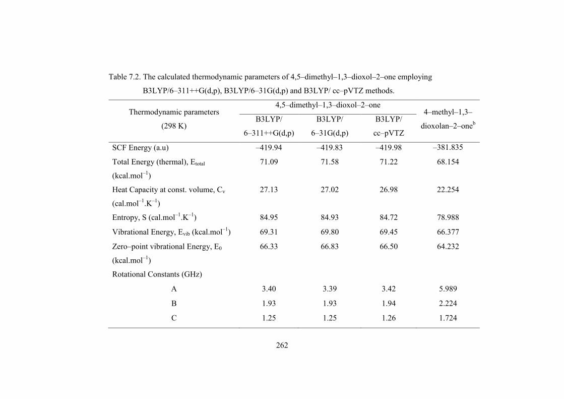
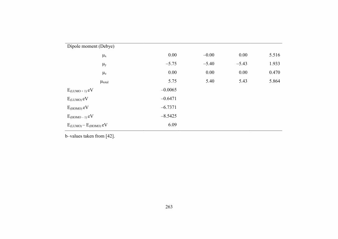
The thermodynamic parameters namely heat capacity, entropy, rotational

constants, dipole moments, vibrational and vibrational zero point energies of the

compounds have also been computed at DFT−B3LYP levels using6−31G(d,p),

6−311++G(d,p) and cc−pVTZ basis sets and are presented in Table 7.2. The energy

of 4,5−dimethyl−1,3−dioxol−2−one is more (−419.94 a.u) than that of

4−methyl−1,3−dioxolan−2−one it is equal to –381.835 a.u. This reveals that

4,5−dimethyl−1,3−dioxol−2−one is more stable than 4−methyl−1,3−dioxolan−2−one

and is due to the planarity of 4,5−dimethyl−1,3−dioxol−2−one molecule. The

thermodynamic data provides helpful information for the further study on the title

compounds, when these may be used as a reactant to take part in a new reaction.

These standard thermodynamic functions can be used as reference thermodynamic

values to calculate changes of entropies (ΔST), changes of enthalpies (ΔHT) and

changes of Gibbs free energies (ΔGT) of the reaction. The dipole moment and its

principal inertial axes are strongly depend upon the conformation of the molecule.

The 4−methyl−1,3−dioxolan−2−one has higher dipole moment (5.864 debye) than

that of 4,5−dimethyl−1,3−dioxol−2−one (5.75 debye). The zero dipole moment in the

z and x axis is due to the C2V point group symmetry of the molecule.

244

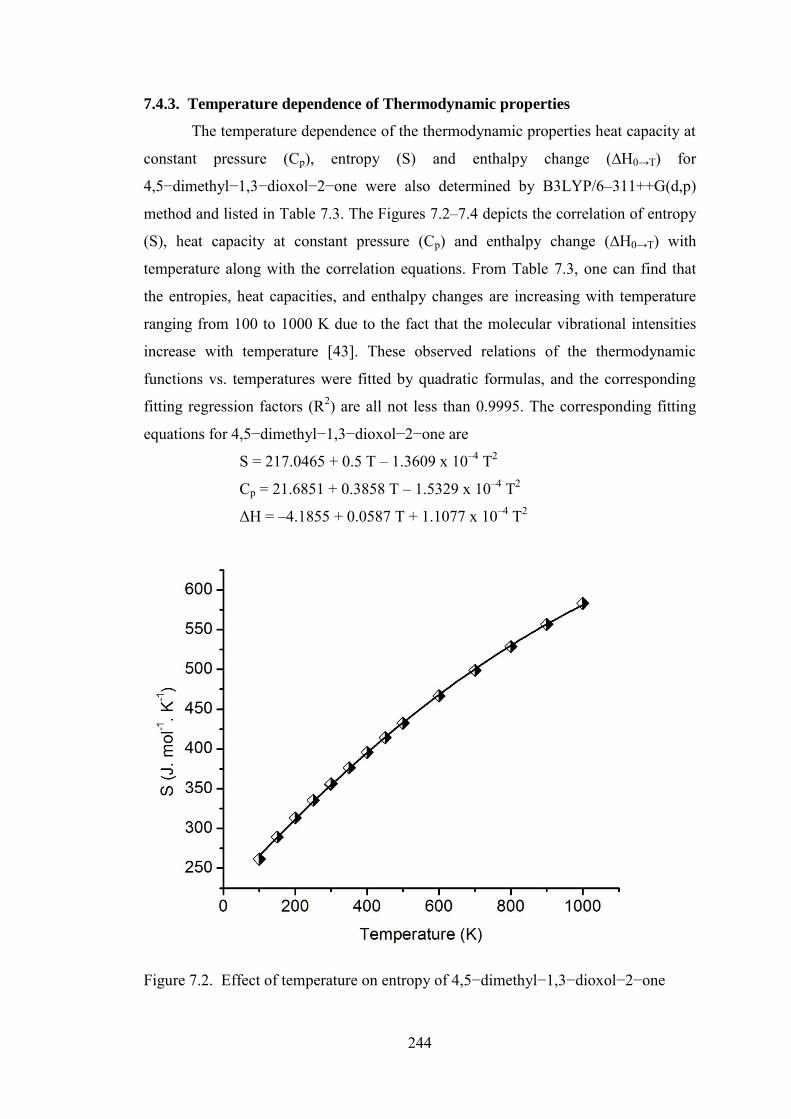
7.4.3. Temperature dependence of Thermodynamic properties

The temperature dependence of the thermodynamic properties heat capacity at

constant pressure (Cp), entropy (S) and enthalpy change (∆H0→T) for

4,5−dimethyl−1,3−dioxol−2−one were also determined by B3LYP/6–311++G(d,p)

method and listed in Table 7.3. The Figures 7.2–7.4 depicts the correlation of entropy

(S), heat capacity at constant pressure (Cp) and enthalpy change (∆H0→T) with

temperature along with the correlation equations. From Table 7.3, one can find that

the entropies, heat capacities, and enthalpy changes are increasing with temperature

ranging from 100 to 1000 K due to the fact that the molecular vibrational intensities

increase with temperature [43]. These observed relations of the thermodynamic

functions vs. temperatures were fitted by quadratic formulas, and the corresponding

fitting regression factors (R2) are all not less than 0.9995. The corresponding fitting

equations for 4,5−dimethyl−1,3−dioxol−2−one are

S = 217.0465 + 0.5 T – 1.3609 x 10–4 T2

Cp = 21.6851 + 0.3858 T – 1.5329 x 10–4 T2

ΔH = –4.1855 + 0.0587 T + 1.1077 x 10–4 T2

Figure 7.2. Effect of temperature on entropy of 4,5−dimethyl−1,3−dioxol−2−one

245

Figure 7.3. Effect of temperature on heat capacity at constant pressure of

4,5−dimethyl−1,3−dioxol−2−one

Figure 7.4. Effect of temperature on enthalpy change (∆H0→T) of

4,5−dimethyl−1,3−dioxol−2−one

246

7.4.4. Analysis of Molecular electrostatic potential (MESP)

The molecular electrostatic potential surface (MESP) which is a method of

mapping electrostatic potential onto the iso–electron density surface simultaneously

displays electrostatic potential (electron + nuclei) distribution, molecular shape, size

and dipole moments of the molecule and it provides a visual method to understand

the relative polarity. Electrostatic potential maps illustrate the charge distributions of

molecules three dimensionally. These maps allow us to visualize variably charged

regions of a molecule. Knowledge of the charge distributions can be used to

determine how molecules interact with one another. One of the purposes of finding

the electrostatic potential is to find the reactive site of a molecule. In the electrostatic

potential map, the semi–spherical blue shapes that emerge from the edges of the

above electrostatic potential map are hydrogen atoms. The molecular electrostatic

potential (MEP) at a point r in the space around a molecule (in atomic units) can be

expressed as:

rr

drr

rR

ZrV

AA

A

'

')'()(

where, ZA is the charge on nucleus A, located at RA and ρ(r′) is the electronic density

function for the molecule. The first and second terms represent the contributions to

the potential due to nuclei and electrons, respectively. V(r) is the resultant at each

point r, which is the net electrostatic effect produced at the point r by both the

electrons and nuclei of the molecule. The total electron density and MESP surfaces of

the molecules under investigation are constructed by using B3LYP/6–311++G(d,p)

method. These pictures illustrate an electrostatic potential model of the compounds,

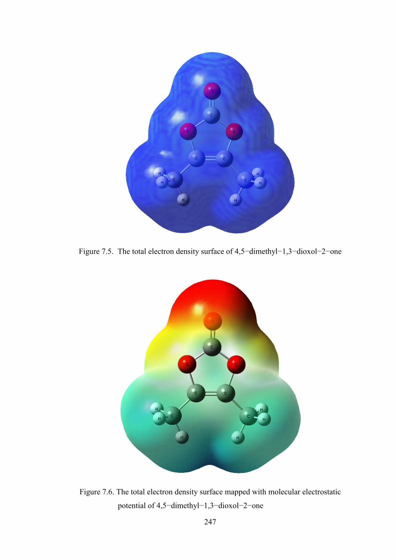
computed at the 0.002 a.u isodensity surface. The total electron density surface of

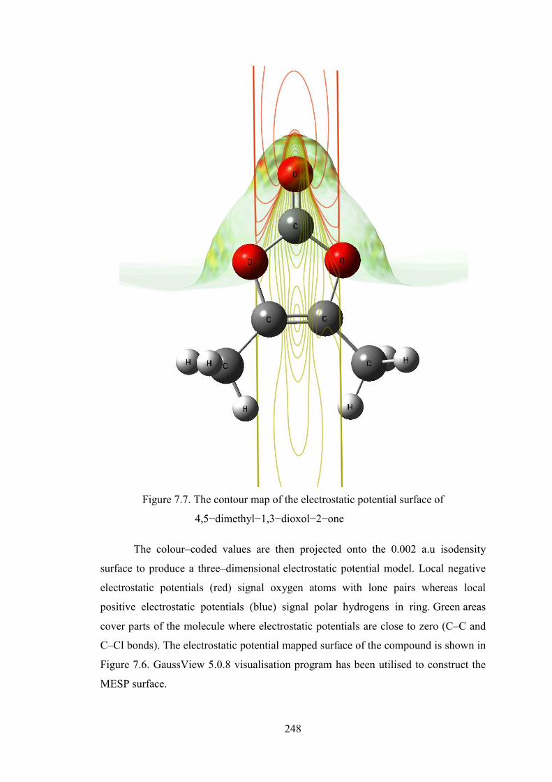
4,5−dimethyl−1,3−dioxol−2−one is depicted in Figure 7.5 while the MESP mapped

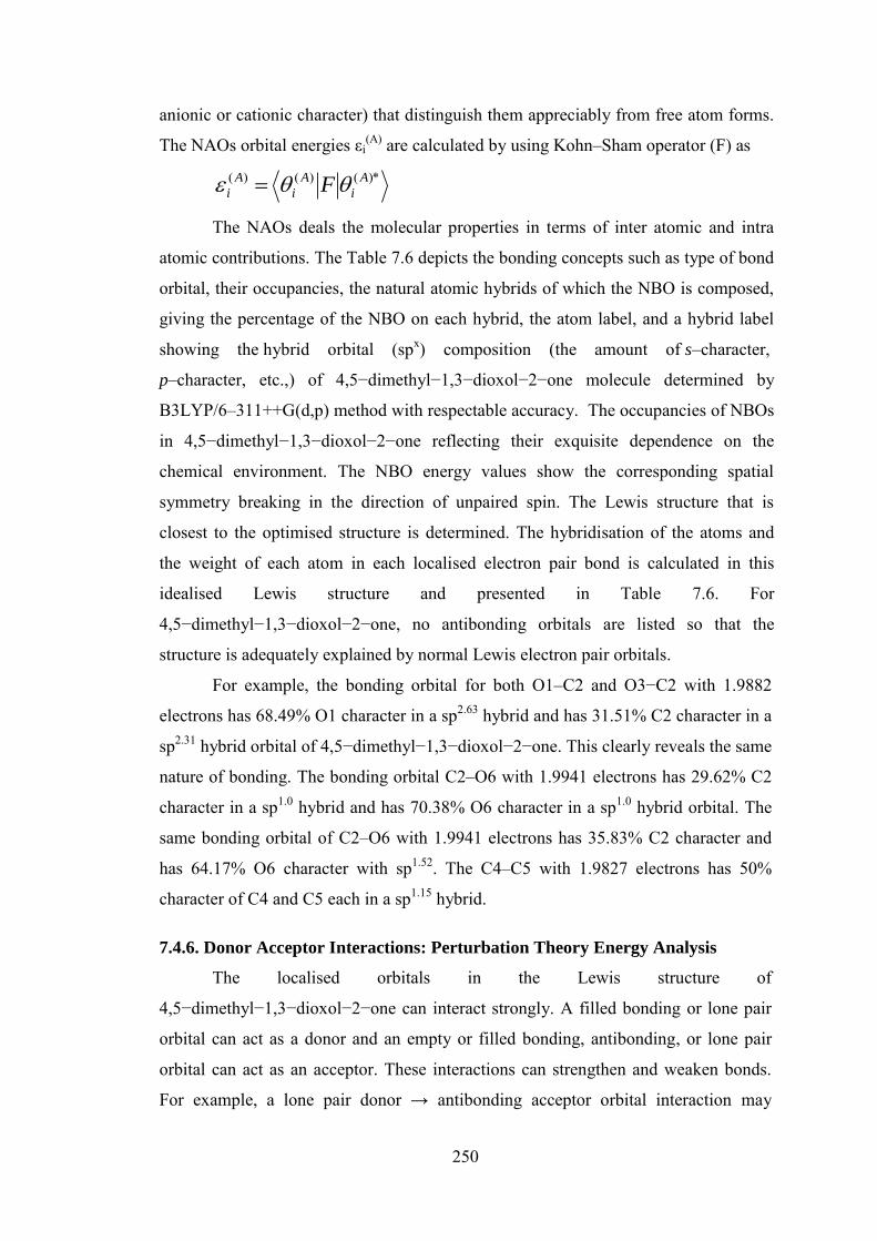
surface of the compound and electrostatic potential contour map for positive and

negative potentials are shown in Figures 7.6 and 7.7. The colour scheme of MESP is

the negative electrostatic potentials are shown in red, the intensity of which is

proportional to the absolute value of the potential energy, and positive electrostatic

potentials are shown in blue while Green indicates surface areas where the potentials

are close to zero. The Figure 7.8 shows the molecular electrostatic potential surface of

4,5−dimethyl−1,3−dioxol−2−one.

247

Figure 7.5. The total electron density surface of 4,5−dimethyl−1,3−dioxol−2−one

Figure 7.6. The total electron density surface mapped with molecular electrostatic

potential of 4,5−dimethyl−1,3−dioxol−2−one

248

Figure 7.7. The contour map of the electrostatic potential surface of

4,5−dimethyl−1,3−dioxol−2−one

The colour–coded values are then projected onto the 0.002 a.u isodensity

surface to produce a three–dimensional electrostatic potential model. Local negative

electrostatic potentials (red) signal oxygen atoms with lone pairs whereas local

positive electrostatic potentials (blue) signal polar hydrogens in ring. Green areas

cover parts of the molecule where electrostatic potentials are close to zero (C–C and

C–Cl bonds). The electrostatic potential mapped surface of the compound is shown in

Figure 7.6. GaussView 5.0.8 visualisation program has been utilised to construct the

MESP surface.

249

Figure 7.8. The molecular electrostatic potential surface of

4,5−dimethyl−1,3−dioxol−2−one

7.4.5. Natural bond orbital analysis

Natural bond orbital (NBO) methods encompass a suite of algorithms that

enable fundamental bonding concepts to be extracted from Hartree‐Fock (HF),

Density Functional Theory (DFT), and post‐HF computations. NBO analysis

originated as a technique for studying hybridisation and covalency effects in

polyatomic wave functions, based on local block eigen vectors of the one–particle

density matrix. NBOs would correspond closely to the picture of localised bonds and

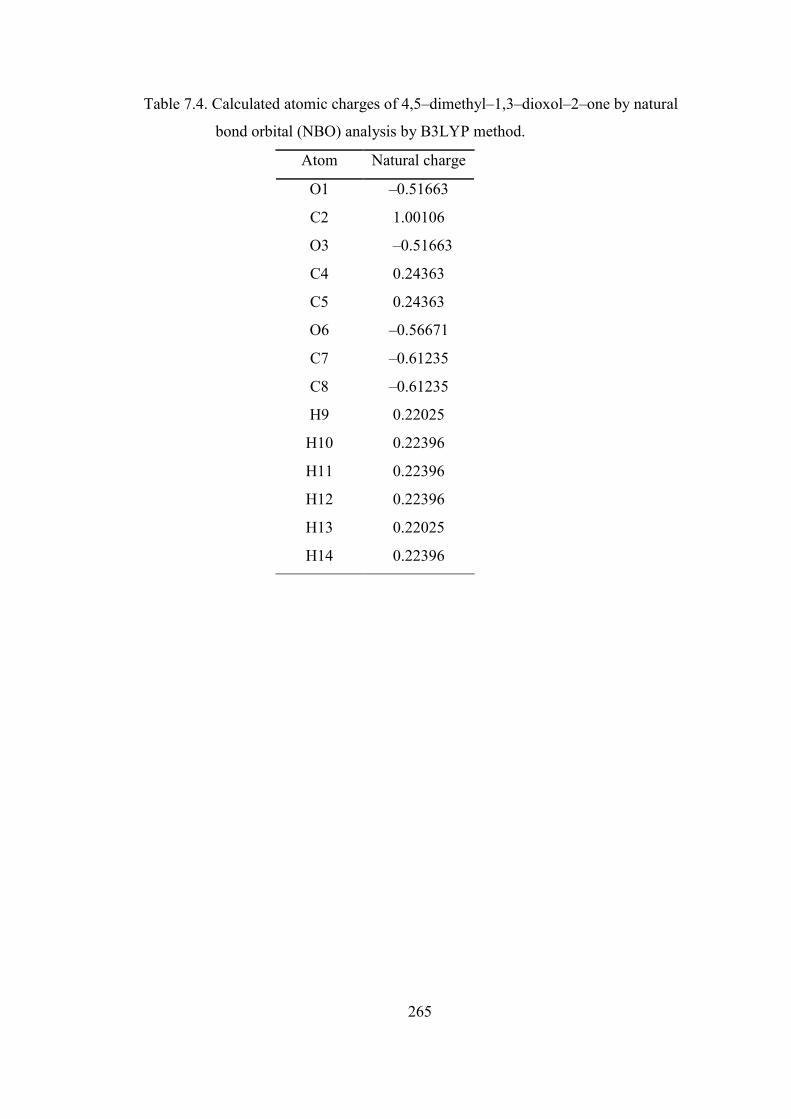
lone pairs as basic units of molecular structure. The atomic charges of

4,5−dimethyl−1,3−dioxol−2−one calculated by NBO analysis using the

B3LYP/6–311++G(d,p) method are presented in Table 7.4. Among the ring oxygen

atoms O1 and O3 have same negative charges. But O6 has more negative charge due

to the resonance of carbonyl group. The charges of C4 and C5 are also same. The

methyl carbon atoms C7 and C8 have negative charge due to hyperconjugative effect

of methyl groups.

In Table 7.5, the natural atomic orbitals, their occupancies and the

corresponding energy of 4,5−dimethyl−1,3−dioxol−2−one were described. In a given

molecular environment the natural atomic orbitals reflect the chemical give and take

of electronic interactions, with variations of shape (e.g., angular deformations due to

steric pressures of adjacent atoms) and size (e.g., altered diffuseness due to increased

250

anionic or cationic character) that distinguish them appreciably from free atom forms.

The NAOs orbital energies εi(A) are calculated by using Kohn–Sham operator (F) as

)*()()( A

i

A

i

A

i F

The NAOs deals the molecular properties in terms of inter atomic and intra

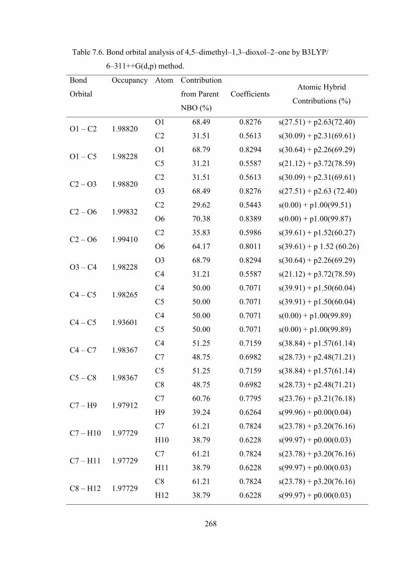
atomic contributions. The Table 7.6 depicts the bonding concepts such as type of bond

orbital, their occupancies, the natural atomic hybrids of which the NBO is composed,

giving the percentage of the NBO on each hybrid, the atom label, and a hybrid label

showing the hybrid orbital (spx) composition (the amount of s–character,

p–character, etc.,) of 4,5−dimethyl−1,3−dioxol−2−one molecule determined by

B3LYP/6–311++G(d,p) method with respectable accuracy. The occupancies of NBOs

in 4,5−dimethyl−1,3−dioxol−2−one reflecting their exquisite dependence on the

chemical environment. The NBO energy values show the corresponding spatial

symmetry breaking in the direction of unpaired spin. The Lewis structure that is

closest to the optimised structure is determined. The hybridisation of the atoms and

the weight of each atom in each localised electron pair bond is calculated in this

idealised Lewis structure and presented in Table 7.6. For

4,5−dimethyl−1,3−dioxol−2−one, no antibonding orbitals are listed so that the

structure is adequately explained by normal Lewis electron pair orbitals.

For example, the bonding orbital for both O1–C2 and O3−C2 with 1.9882

electrons has 68.49% O1 character in a sp2.63 hybrid and has 31.51% C2 character in a

sp2.31 hybrid orbital of 4,5−dimethyl−1,3−dioxol−2−one. This clearly reveals the same

nature of bonding. The bonding orbital C2–O6 with 1.9941 electrons has 29.62% C2

character in a sp1.0 hybrid and has 70.38% O6 character in a sp1.0 hybrid orbital. The

same bonding orbital of C2–O6 with 1.9941 electrons has 35.83% C2 character and

has 64.17% O6 character with sp1.52. The C4–C5 with 1.9827 electrons has 50%

character of C4 and C5 each in a sp1.15 hybrid.

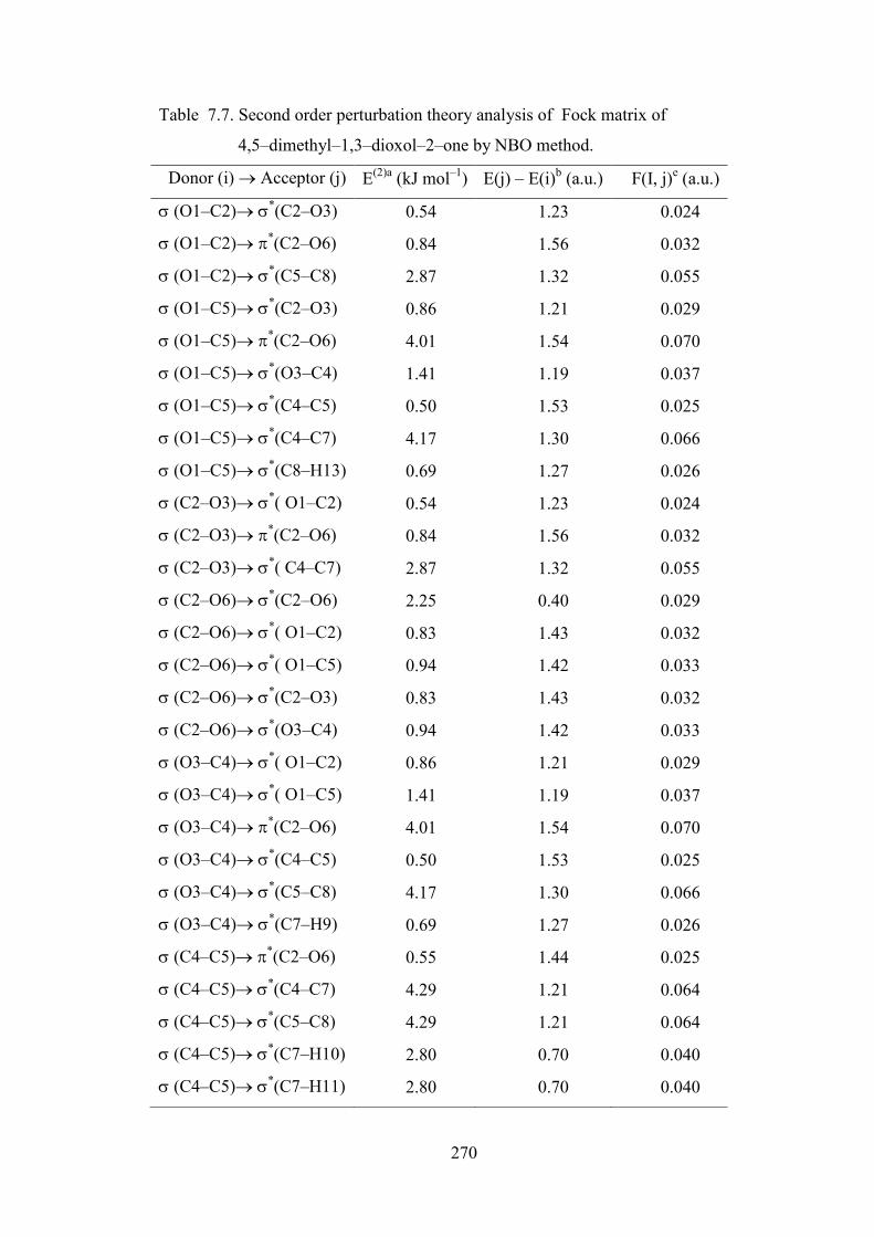
7.4.6. Donor Acceptor Interactions: Perturbation Theory Energy Analysis

The localised orbitals in the Lewis structure of

4,5−dimethyl−1,3−dioxol−2−one can interact strongly. A filled bonding or lone pair

orbital can act as a donor and an empty or filled bonding, antibonding, or lone pair

orbital can act as an acceptor. These interactions can strengthen and weaken bonds.

For example, a lone pair donor → antibonding acceptor orbital interaction may

251

weaken the bond associated with the antibonding orbital. Conversely, an interaction

with a bonding pair as the acceptor may strengthen the bond. Strong electron

delocalisation in the Lewis structure also shows up as donor–acceptor interactions.

The stabilisation energy of different kinds of interactions are listed Table 7.7. This

calculation is done by examining all possible interactions between ‘filled’ (donor)

Lewis–type NBOs and ‘empty’ (acceptor) non–Lewis NBOs, and estimating their

energetic importance by 2nd–order perturbation theory. Since these interactions lead to

loss of occupancy from the localised NBOs of the idealised Lewis structure into the

empty non–Lewis orbitals (and thus, to departures from the idealised Lewis structure

description), they are referred to as ‘delocalisation’ corrections to the natural Lewis

structure.

The NBO method demonstrates the bonding concepts like atomic charge,

Lewis structure, bond type, hybridization, bond order, charge transfer and resonance

weights. Natural bond orbital (NBO) analysis is a useful tool for understanding

delocalisation of electron density from occupied Lewis–type (donor) NBOs to

properly unoccupied non–Lewis type (acceptor) NBOs within the molecule. The

stabilisation of orbital interaction is proportional to the energy difference between

interacting orbitals. Therefore, the interaction having strongest stabilisation takes

place between effective donors and effective acceptors. This bonding–anti bonding

interaction can be quantitatively described in terms of the NBO approach that is

expressed by means of second–order perturbation interaction energy E(2) [65–68]. This

energy represents the estimate of the off–diagonal NBO Fock matrix element. The

stabilisation energy E(2) associated with i (donor) → j (acceptor) delocalisation is

estimated from the second–order perturbation approach as [68] given below

ij

i

jiFqE

),(2)2(

where, qi is the donor orbital occupancy, εi and εj are diagonal elements (orbital

energies) and F(i,j) is the off–diagonal Fock matrix element.

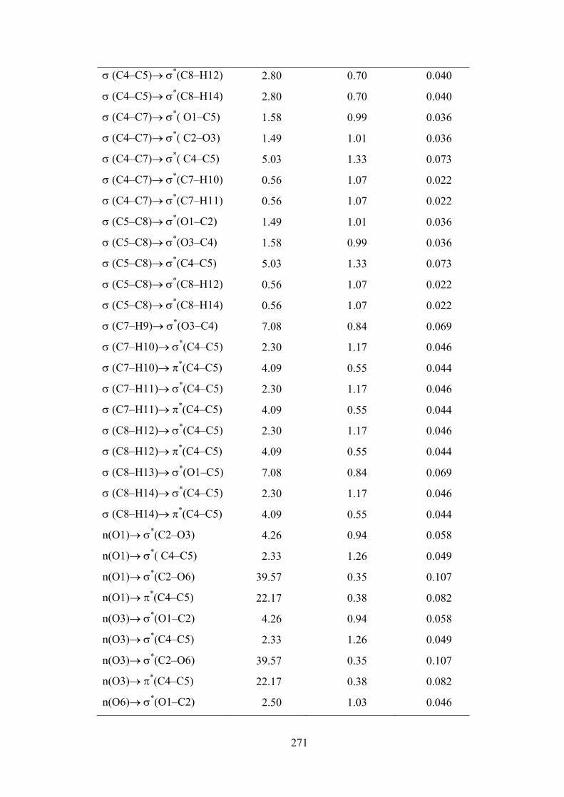
In 4,5−dimethyl−1,3−dioxol−2−one molecule, the bond pair donor

orbital, σOC → π*CO interaction between the O1–C5 bond pair and the antiperiplanar

C2–O6 antibonding orbital give stabilisation of 4.01 kJ. mol–1. The bond pair donor

orbital, σCC → σ*CC interaction between the C4–C5 bond pair and the antiperiplanar

C4–C7 and C5−C8 antibonding orbital give equal stabilisation of 2.8 kJ. mol–1. The

252

lone pair donor orbital, nO → σ*CO interaction between the O1 and O3 oxygen lone

pair and the antiperiplanar C2–O6 antibonding orbital is seen to give a strong

stabilisation, 39.57 kJ. mol−1. The lone pair donor orbital, nO → σ*OC interaction

between the oxygen O6 lone pair and the antiperiplanar O1–C2 and C2−O3

antibonding orbital is seen to give a strong and equal stabilisation, 32.48 kJ. mol−1.

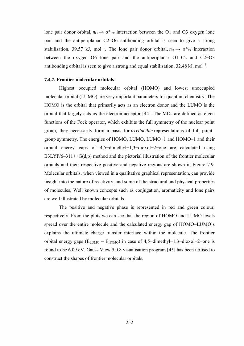
7.4.7. Frontier molecular orbitals

Highest occupied molecular orbital (HOMO) and lowest unoccupied

molecular orbital (LUMO) are very important parameters for quantum chemistry. The

HOMO is the orbital that primarily acts as an electron donor and the LUMO is the

orbital that largely acts as the electron acceptor [44]. The MOs are defined as eigen

functions of the Fock operator, which exhibits the full symmetry of the nuclear point

group, they necessarily form a basis for irreducible representations of full point–

group symmetry. The energies of HOMO, LUMO, LUMO+1 and HOMO–1 and their

orbital energy gaps of 4,5−dimethyl−1,3−dioxol−2−one are calculated using

B3LYP/6–311++G(d,p) method and the pictorial illustration of the frontier molecular

orbitals and their respective positive and negative regions are shown in Figure 7.9.

Molecular orbitals, when viewed in a qualitative graphical representation, can provide

insight into the nature of reactivity, and some of the structural and physical properties

of molecules. Well known concepts such as conjugation, aromaticity and lone pairs

are well illustrated by molecular orbitals.

The positive and negative phase is represented in red and green colour,

respectively. From the plots we can see that the region of HOMO and LUMO levels

spread over the entire molecule and the calculated energy gap of HOMO–LUMO’s

explains the ultimate charge transfer interface within the molecule. The frontier

orbital energy gaps (ELUMO – EHOMO) in case of 4,5−dimethyl−1,3−dioxol−2−one is

found to be 6.09 eV. Gauss View 5.0.8 visualisation program [45] has been utilised to

construct the shapes of frontier molecular orbitals.

253

Figure 7.9. The frontier molecular orbitals of 4,5−dimethyl−1,3−dioxol−2−one

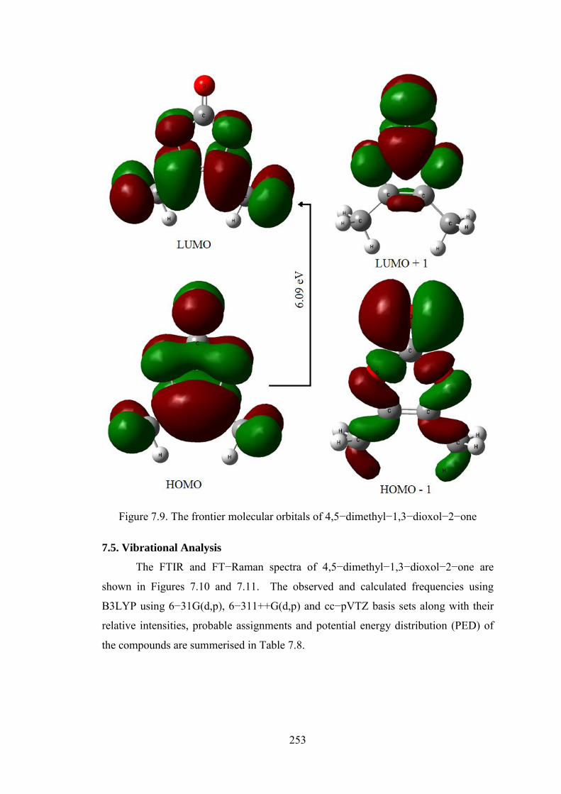
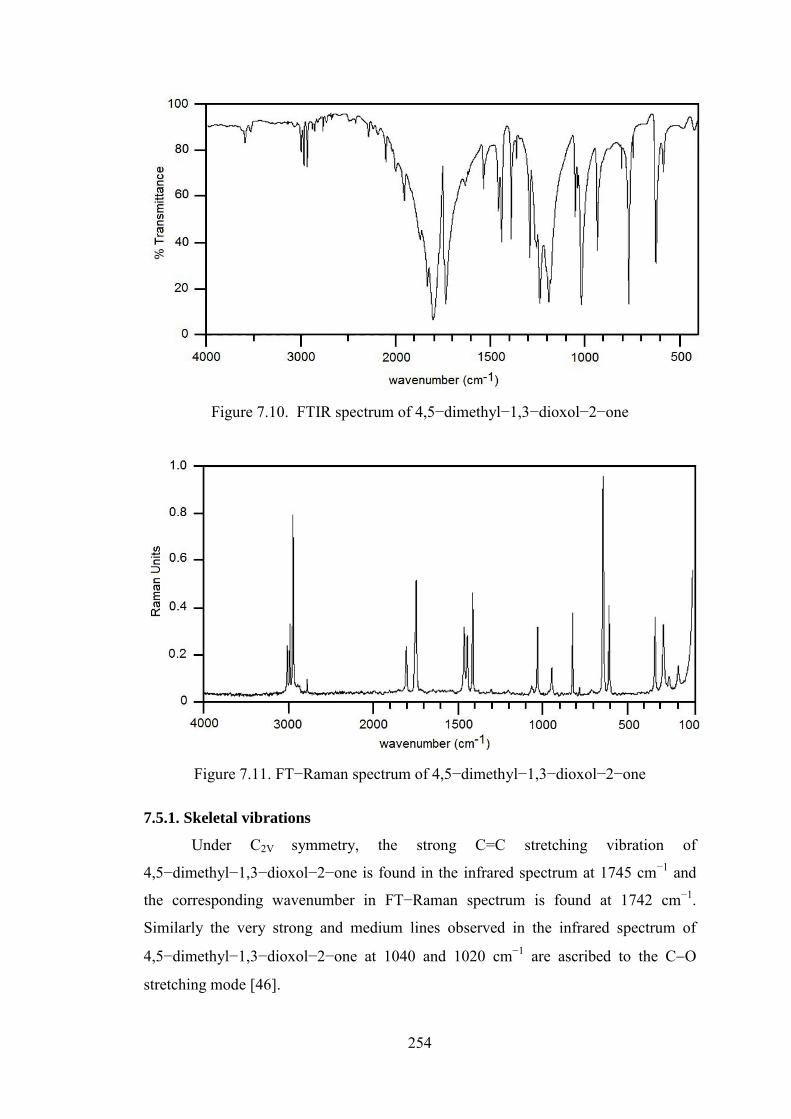
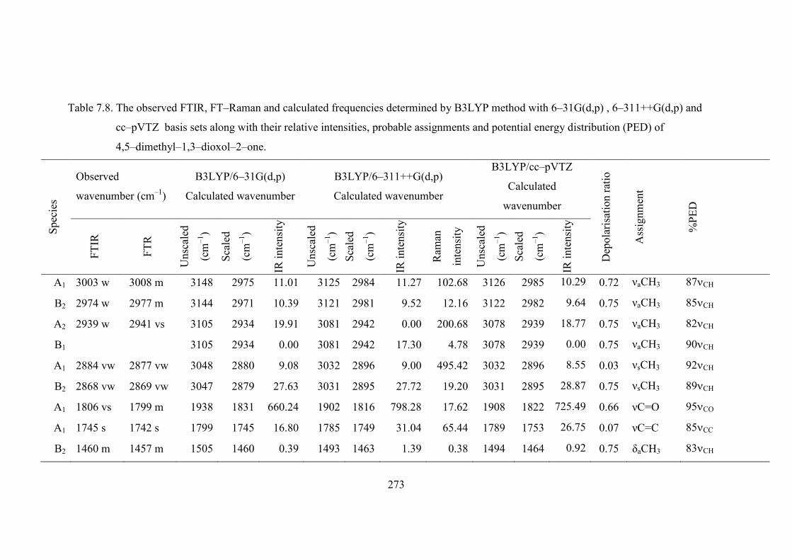
7.5. Vibrational Analysis

The FTIR and FT−Raman spectra of 4,5−dimethyl−1,3−dioxol−2−one are

shown in Figures 7.10 and 7.11. The observed and calculated frequencies using

B3LYP using 6−31G(d,p), 6−311++G(d,p) and cc−pVTZ basis sets along with their

relative intensities, probable assignments and potential energy distribution (PED) of

the compounds are summerised in Table 7.8.

254

Figure 7.10. FTIR spectrum of 4,5−dimethyl−1,3−dioxol−2−one

Figure 7.11. FT−Raman spectrum of 4,5−dimethyl−1,3−dioxol−2−one

7.5.1. Skeletal vibrations

Under C2V symmetry, the strong C=C stretching vibration of

4,5−dimethyl−1,3−dioxol−2−one is found in the infrared spectrum at 1745 cm−1 and

the corresponding wavenumber in FT−Raman spectrum is found at 1742 cm−1.

Similarly the very strong and medium lines observed in the infrared spectrum of

4,5−dimethyl−1,3−dioxol−2−one at 1040 and 1020 cm−1 are ascribed to the CO

stretching mode [46].

255

The fundamental modes observed at 1256 cm−1 in the infrared is attributed to

the OCO asymmetric stretching and at 1241 cm−1 is assigned to the OCO symmetric

stretching modes of 4,5−dimethyl−1,3−dioxol−2−one [47]. The bands occurring at

770 cm−1 in the infrared and the theoretical value of 630 cm−1 are assigned to the OCO

and COC in−plane bending modes of 4,5−dimethyl−1,3−dioxol−2−one. The COC and

OCC out of plane bending modes of 4,5−dimethyl−1,3−dioxol−2−one under C2V

symmetry are attributed to the Raman wavenumbers 320 and 266 cm−1. The in−plane

bending and out of plane vibrations are described as mixed modes as there are about

15 to 25% PED contributions mainly from C=O and CCO in−plane bending and out

of plane bending vibrations, respectively.

7.5.2. C=O vibrations

The C=O stretch lies in the spectral range 1750−1860 cm−1, and is very intense

in the infrared and only moderately active in Raman. In

4,5−dimethyl−1,3−dioxol−2−one the carbonyl stretching frequency is observed in the

high frequency region as a very strong band at 1806 cm−1 in IR and medium band at

1799 m−1 in Raman spectra. In 4−methyl−l,3−dioxolan−2−one, the carbonyl

stretching frequency is observed as a very strong band at 1790 cm−1 in IR and in

Raman spectra [42].The fundamental mode at 587 cm−1 in the infrared spectrum is

attributed to the C=O in−plane bending of 4,5−dimethyl−1,3−dioxol−2−one. The

wavenumber observed at 626 cm−1 in the infrared and at 632 cm−1 in Raman spectra

of are assigned to the C=O out of plane bending vibration. The C=O out of plane

bending of 4,5−dimethyl−1,3−dioxolan−2−one is observed at 820 cm−1 in IR

spectrum as a strong bands. The in−plane and out of plane bending of the carbonyl

group is mixed significantly with the in−plane and out of plane bending vibrations of

OCO vibration.

7.5.3. Methyl group vibrations

The asymmetric stretching and asymmetric deformation modes of the −CH3

group would be expected to be depolarised. The νs(CH3) frequencies are established

at 2884 and 2868 cm−1 in the infrared spectrum and νa(CH3) is assigned at 3033, 2974

and 2939 cm−1 of 4,5−dimethyl−1,3−dioxol−2−one. The –CH3 twist, rock and

deformation motions and the vibrations of the ring moieties are found in the spectral

region 900−1500 cm−1. The symmetrical methyl deformational mode is obtained at

256

1392 and 1293 cm−1 in IR spectrum as strong modes. The asymmetrical methyl

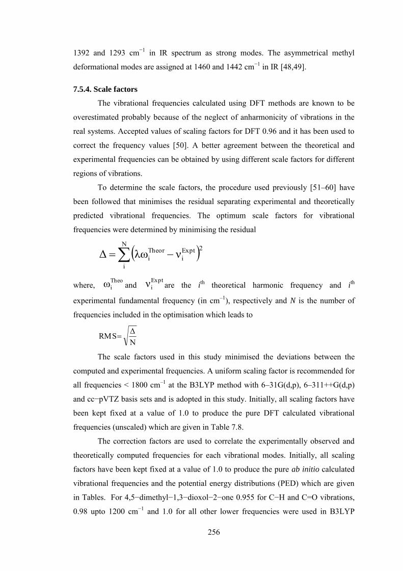
deformational modes are assigned at 1460 and 1442 cm−1 in IR [48,49].

7.5.4. Scale factors

The vibrational frequencies calculated using DFT methods are known to be

overestimated probably because of the neglect of anharmonicity of vibrations in the

real systems. Accepted values of scaling factors for DFT 0.96 and it has been used to

correct the frequency values [50]. A better agreement between the theoretical and

experimental frequencies can be obtained by using different scale factors for different

regions of vibrations.

To determine the scale factors, the procedure used previously [51–60] have

been followed that minimises the residual separating experimental and theoretically

predicted vibrational frequencies. The optimum scale factors for vibrational

frequencies were determined by minimising the residual

N

i

2Expti

Theori νλωΔ

where, Theoiω and

Exptiν are the i

th theoretical harmonic frequency and ith

experimental fundamental frequency (in cm–1), respectively and N is the number of

frequencies included in the optimisation which leads to

NΔRMS

The scale factors used in this study minimised the deviations between the

computed and experimental frequencies. A uniform scaling factor is recommended for

all frequencies < 1800 cm–1 at the B3LYP method with 6–31G(d,p), 6–311++G(d,p)

and cc−pVTZ basis sets and is adopted in this study. Initially, all scaling factors have

been kept fixed at a value of 1.0 to produce the pure DFT calculated vibrational

frequencies (unscaled) which are given in Table 7.8.

The correction factors are used to correlate the experimentally observed and

theoretically computed frequencies for each vibrational modes. Initially, all scaling

factors have been kept fixed at a value of 1.0 to produce the pure ab initio calculated

vibrational frequencies and the potential energy distributions (PED) which are given

in Tables. For 4,5−dimethyl−1,3−dioxol−2−one 0.955 for C−H and C=O vibrations,

0.98 upto 1200 cm−1 and 1.0 for all other lower frequencies were used in B3LYP

257

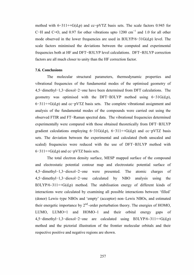
method with 6−311++G(d,p) and cc−pVTZ basis sets. The scale factors 0.945 for

C−H and C=O, and 0.97 for other vibrations upto 1200 cm−1 and 1.0 for all other

mode observed in the lower frequencies are used in B3LYP/6−31G(d,p) level. The

scale factors minimised the deviations between the computed and experimental

frequencies both at HF and DFT−B3LYP level calculations. DFT−B3LYP correction

factors are all much closer to unity than the HF correction factor.

7.6. Conclusions

The molecular structural parameters, thermodynamic properties and

vibrational frequencies of the fundamental modes of the optimised geometry of

4,5−dimethyl−1,3−dioxol−2−one have been determined from DFT calculations. The

geometry was optimised with the DFT−B3LYP method using 6−31G(d,p),

6−311++G(d,p) and cc−pVTZ basis sets. The complete vibrational assignment and

analysis of the fundamental modes of the compounds were carried out using the

observed FTIR and FT−Raman spectral data. The vibrational frequencies determined

experimentally were compared with those obtained theoretically from DFT−B3LYP

gradient calculations employing 6−31G(d,p), 6−311++G(d,p) and cc−pVTZ basis

sets. The deviation between the experimental and calculated (both unscaled and

scaled) frequencies were reduced with the use of DFT−B3LYP method with

6−311++G(d,p) and cc−pVTZ basis sets.

The total electron density surface, MESP mapped surface of the compound

and electrostatic potential contour map and electrostatic potential surface of

4,5−dimethyl−1,3−dioxol−2−one were presented. The atomic charges of

4,5−dimethyl−1,3−dioxol−2−one calculated by NBO analysis using the

B3LYP/6–311++G(d,p) method. The stabilisation energy of different kinds of

interactions were calculated by examining all possible interactions between ‘filled’

(donor) Lewis–type NBOs and ‘empty’ (acceptor) non–Lewis NBOs, and estimated

their energetic importance by 2nd–order perturbation theory. The energies of HOMO,

LUMO, LUMO+1 and HOMO–1 and their orbital energy gaps of

4,5−dimethyl−1,3−dioxol−2−one are calculated using B3LYP/6–311++G(d,p)

method and the pictorial illustration of the frontier molecular orbitals and their

respective positive and negative regions are shown.

258

Table 7.1. Structural parameters calculated for 4,5–dimethyl–1,3–dioxol–2–one employing B3LYP/6–311++G(d,p),

B3LYP/6–31G(d,p) and B3LYP/ cc–pVTZ methods.

Structural

Parameters

4,5–dimethyl–1,3–dioxol–2–one

Expermentala

B3LYP/

6–311++G(d,p)

B3LYP/

6–31G(d,p)

B3LYP/

cc–pVTZ

4–methyl–1,3–

dioxolan–2–oneb

Internuclear Distance (Ǻ)

O1–C2 1.37 1.37 1.36 1.358 1.362

O1–C5 1.40 1.40 1.40 1.428 1.436

C2–O3 1.37 1.37 1.36 1.358 1.358

C2–O6 1.19 1.20 1.19 1.200 1.189

O3–C4 1.40 1.40 1.40 1.428 1.448

C4–C5 1.33 1.34 1.33 1.540 1.533

C4–C7 1.48 1.48 1.48 1.514

C5–C8 1.48 1.48 1.48 1.514

C7–H (methyl)c 1.09 1.09 1.09

C8–H (methyl)c 1.09 1.10 1.09

Bond Angle (degree)

C2–O1–C5 107.9 107.8 107.8 109.3

O1–C2–O3 107.8 107.9 107.8 111.67 110.2

259

O1–C2–O6 126.1 126.1 126.1 124.7

O3–C2–O6 126.1 126.1 126.1 124.17 125.1

C2–O3–C4 107.9 107.8 107.8 108.71 109.9

O3–C4–C5 108.2 108.3 108.3 102.16 101.8

O3–C4–C7 117.0 117.0 117.0 110.4

C5–C4–C7 134.8 134.7 134.8 115.7

O1–C5–C4 108.2 108.3 108.3 103.3

O1–C5–C8 117.0 117.0 117.0

C4–C5–C8 134.8 134.7 134.8 115.7

C4–C7–H9 110.3 110.3 110.4

C4–C7–H10 110.9 111.0 110.9

C4–C7–H11 110.9 111.0 110.9

H9–C7–H10 108.4 108.4 108.4

H9–C7–H11 108.4 108.4 108.4

H10–C7–H11 107.8 107.6 107.6

C5–C8–H12 110.9 111.0 110.9

C5–C8–H13 110.3 110.3 110.4

C5–C8–H14 110.9 111.0 110.9

H12–C8–H13 108.4 108.4 108.4

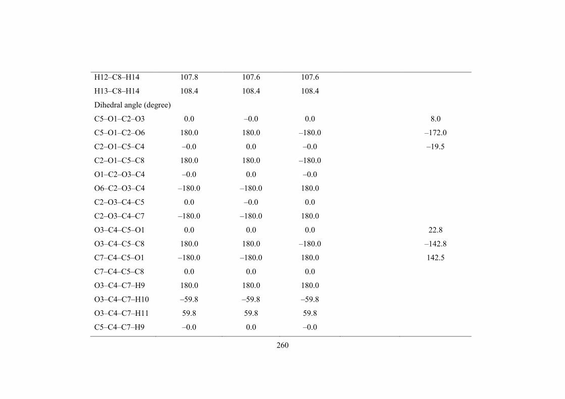
260

H12–C8–H14 107.8 107.6 107.6

H13–C8–H14 108.4 108.4 108.4

Dihedral angle (degree)

C5–O1–C2–O3 0.0 –0.0 0.0 8.0

C5–O1–C2–O6 180.0 180.0 –180.0 –172.0

C2–O1–C5–C4 –0.0 0.0 –0.0 –19.5

C2–O1–C5–C8 180.0 180.0 –180.0

O1–C2–O3–C4 –0.0 0.0 –0.0

O6–C2–O3–C4 –180.0 –180.0 180.0

C2–O3–C4–C5 0.0 –0.0 0.0

C2–O3–C4–C7 –180.0 –180.0 180.0

O3–C4–C5–O1 0.0 0.0 0.0 22.8

O3–C4–C5–C8 180.0 180.0 –180.0 –142.8

C7–C4–C5–O1 –180.0 –180.0 180.0 142.5

C7–C4–C5–C8 0.0 0.0 0.0

O3–C4–C7–H9 180.0 180.0 180.0

O3–C4–C7–H10 –59.8 –59.8 –59.8

O3–C4–C7–H11 59.8 59.8 59.8

C5–C4–C7–H9 –0.0 0.0 –0.0

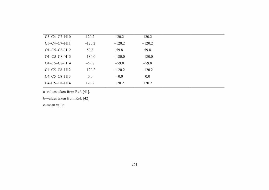
261

C5–C4–C7–H10 120.2 120.2 120.2

C5–C4–C7–H11 –120.2 –120.2 –120.2

O1–C5–C8–H12 59.8 59.8 59.8

O1–C5–C8–H13 –180.0 –180.0 –180.0

O1–C5–C8–H14 –59.8 –59.8 –59.8

C4–C5–C8–H12 –120.2 –120.2 –120.2

C4–C5–C8–H13 0.0 –0.0 0.0

C4–C5–C8–H14 120.2 120.2 120.2

a–values taken from Ref. [41].

b–values taken from Ref. [42]

c–mean value

262

Table 7.2. The calculated thermodynamic parameters of 4,5–dimethyl–1,3–dioxol–2–one employing

B3LYP/6–311++G(d,p), B3LYP/6–31G(d,p) and B3LYP/ cc–pVTZ methods.

Thermodynamic parameters

(298 K)

4,5–dimethyl–1,3–dioxol–2–one 4–methyl–1,3–

dioxolan–2–oneb B3LYP/

6–311++G(d,p)

B3LYP/

6–31G(d,p)

B3LYP/

cc–pVTZ

SCF Energy (a.u) –419.94 –419.83 –419.98 –381.835

Total Energy (thermal), Etotal

(kcal.mol–1)

71.09 71.58 71.22 68.154

Heat Capacity at const. volume, Cv

(cal.mol–1.K–1)

27.13 27.02 26.98 22.254

Entropy, S (cal.mol–1.K–1) 84.95 84.93 84.72 78.988

Vibrational Energy, Evib (kcal.mol–1) 69.31 69.80 69.45 66.377

Zero–point vibrational Energy, E0

(kcal.mol–1)

66.33 66.83 66.50 64.232

Rotational Constants (GHz)

A 3.40 3.39 3.42 5.989

B 1.93 1.93 1.94 2.224

C 1.25 1.25 1.26 1.724

263

Dipole moment (Debye)

μx 0.00 –0.00 0.00 5.516

μy –5.75 –5.40 –5.43 1.933

μz 0.00 0.00 0.00 0.470

μtotal 5.75 5.40 5.43 5.864

E(LUMO + 1) eV –0.0065

E(LUMO) eV –0.6471

E(HOMO) eV –6.7371

E(HOMO – 1) eV –8.5425

E(LUMO) – E(HOMO) eV 6.09

b–values taken from [42].

264

Table 7.3. Thermodynamic properties of 4,5–dimethyl–1,3–dioxol–2–one determined

at different temperatures with B3LYP/6–311++G(d,p) level.

T (K) S (J.mol–1.K–1) Cp (J.mol–1.K–1) ΔH0→T (kJ.mol–1)

100 261.4 60.32 4.23

150 289.1 76.88 7.68

200 313.28 91.9 11.9

250 335.41 107.05 16.87

298.15 355.53 121.83 22.38

300 356.28 122.39 22.61

350 376.29 137.48 29.11

400 395.59 151.86 36.34

450 414.27 165.27 44.28

500 432.33 177.59 52.85

600 466.66 199.03 71.72

700 498.72 216.78 92.53

800 528.66 231.56 114.97

900 556.67 243.99 138.77

1000 582.94 254.51 163.71

265

Table 7.4. Calculated atomic charges of 4,5–dimethyl–1,3–dioxol–2–one by natural

bond orbital (NBO) analysis by B3LYP method.

Atom Natural charge

O1 –0.51663

C2 1.00106

O3 –0.51663

C4 0.24363

C5 0.24363

O6 –0.56671

C7 –0.61235

C8 –0.61235

H9 0.22025

H10 0.22396

H11 0.22396

H12 0.22396

H13 0.22025

H14 0.22396

266

Table 7.5. The atomic orbital occupancies of 4,5–dimethyl–2,3–dioxol–2–one

Atom No. Atomic orbital Type Occupancy Energy

O1

1s Core 1.99971 –18.99204

2s Valence 1.63436 –0.93158

2px Valence 1.76730 –0.35680

2py Valence 1.40965 –0.34915

2pz Valence 1.69000 –0.37852

C2

1s Core 1.99953 –10.25242

2s Valence 0.67550 –0.13403

2px Valence 0.81706 –0.15954

2py Valence 0.75127 –0.02854

2pz Valence 0.70209 –0.05004

O3

1s Core 1.99971 –18.99204

2s Valence 1.63436 –0.93158

2px Valence 1.76730 –0.35680

2py Valence 1.40965 –0.34915

2pz Valence 1.69000 –0.37852

C4

1s Core 1.99873 –10.12217

2s Valence 0.85058 –0.17321

2px Valence 1.06917 –0.14974

2py Valence 0.76377 –0.07091

2pz Valence 1.05195 –0.09131

C5

1s Core 1.99873 –10.12217

2s Valence 0.85058 –0.17321

2px Valence 1.06917 –0.14974

2py Valence 0.76377 –0.07091

2pz Valence 1.05195 –0.09131

O6

1s Core 1.99971 –18.84489

2s Valence 1.70454 –0.90472

2px Valence 1.49898 –0.26153

2py Valence 1.55432 –0.30957

267

2pz Valence 1.79645 –0.26747

C7

1s Core 1.99927 –10.05757

2s Valence 1.08226 –0.26862

2px Valence 1.22580 –0.12832

2py Valence 1.14334 –0.12239

2pz Valence 1.15292 –0.12310

C8

1s Core 1.99927 –10.05757

2s Valence 1.08226 –0.26862

2px Valence 1.22580 –0.12832

2py Valence 1.14334 –0.12239

2pz Valence 1.15292 –0.12310

H9 1s Valence 0.77830 0.00816

H10 1s Valence 0.77396 0.01584

H11 1s Valence 0.77396 0.01584

H12 1s Valence 0.77396 0.01584

H13 1s Valence 0.77830 0.00816

H14 1s Valence 0.77396 0.01584

268

Table 7.6. Bond orbital analysis of 4,5–dimethyl–1,3–dioxol–2–one by B3LYP/

6–311++G(d,p) method.

Bond

Orbital

Occupancy Atom Contribution

from Parent

NBO (%)

Coefficients Atomic Hybrid

Contributions (%)

O1 – C2 1.98820 O1 68.49 0.8276 s(27.51) + p2.63(72.40)

C2 31.51 0.5613 s(30.09) + p2.31(69.61)

O1 – C5 1.98228 O1 68.79 0.8294 s(30.64) + p2.26(69.29)

C5 31.21 0.5587 s(21.12) + p3.72(78.59)

C2 – O3 1.98820 C2 31.51 0.5613 s(30.09) + p2.31(69.61)

O3 68.49 0.8276 s(27.51) + p2.63 (72.40)

C2 – O6 1.99832 C2 29.62 0.5443 s(0.00) + p1.00(99.51)

O6 70.38 0.8389 s(0.00) + p1.00(99.87)

C2 – O6 1.99410 C2 35.83 0.5986 s(39.61) + p1.52(60.27)

O6 64.17 0.8011 s(39.61) + p 1.52 (60.26)

O3 – C4 1.98228 O3 68.79 0.8294 s(30.64) + p2.26(69.29)

C4 31.21 0.5587 s(21.12) + p3.72(78.59)

C4 – C5 1.98265 C4 50.00 0.7071 s(39.91) + p1.50(60.04)

C5 50.00 0.7071 s(39.91) + p1.50(60.04)

C4 – C5 1.93601 C4 50.00 0.7071 s(0.00) + p1.00(99.89)

C5 50.00 0.7071 s(0.00) + p1.00(99.89)

C4 – C7 1.98367 C4 51.25 0.7159 s(38.84) + p1.57(61.14)

C7 48.75 0.6982 s(28.73) + p2.48(71.21)

C5 – C8 1.98367 C5 51.25 0.7159 s(38.84) + p1.57(61.14)

C8 48.75 0.6982 s(28.73) + p2.48(71.21)

C7 – H9 1.97912 C7 60.76 0.7795 s(23.76) + p3.21(76.18)

H9 39.24 0.6264 s(99.96) + p0.00(0.04)

C7 – H10 1.97729 C7 61.21 0.7824 s(23.78) + p3.20(76.16)

H10 38.79 0.6228 s(99.97) + p0.00(0.03)

C7 – H11 1.97729 C7 61.21 0.7824 s(23.78) + p3.20(76.16)

H11 38.79 0.6228 s(99.97) + p0.00(0.03)

C8 – H12 1.97729 C8 61.21 0.7824 s(23.78) + p3.20(76.16)

H12 38.79 0.6228 s(99.97) + p0.00(0.03)

269

C8 – H13 1.97912 C8 60.76 0.7795 s(23.76) + p3.21(76.18)

H13 39.24 0.6264 s(99.96) + p0.00(0.04)

C8 – H14 1.97729 C8 61.21 0.7824 s(23.78) + p3.20(76.16)

H14 38.79 0.6228 s(99.97) + p0.00(0.03)

270

Table 7.7. Second order perturbation theory analysis of Fock matrix of

4,5–dimethyl–1,3–dioxol–2–one by NBO method.

Donor (i) Acceptor (j) E(2)a (kJ mol–1) E(j) – E(i)b (a.u.) F(I, j)e (a.u.)

(O1–C2) *(C2–O3) 0.54 1.23 0.024

(O1–C2) *(C2–O6) 0.84 1.56 0.032

(O1–C2) *(C5–C8) 2.87 1.32 0.055

(O1–C5) *(C2–O3) 0.86 1.21 0.029

(O1–C5) *(C2–O6) 4.01 1.54 0.070

(O1–C5) *(O3–C4) 1.41 1.19 0.037

(O1–C5) *(C4–C5) 0.50 1.53 0.025

(O1–C5) *(C4–C7) 4.17 1.30 0.066

(O1–C5) *(C8–H13) 0.69 1.27 0.026

(C2–O3) *( O1–C2) 0.54 1.23 0.024

(C2–O3) *(C2–O6) 0.84 1.56 0.032

(C2–O3) *( C4–C7) 2.87 1.32 0.055

(C2–O6) *(C2–O6) 2.25 0.40 0.029

(C2–O6) *( O1–C2) 0.83 1.43 0.032

(C2–O6) *( O1–C5) 0.94 1.42 0.033

(C2–O6) *(C2–O3) 0.83 1.43 0.032

(C2–O6) *(O3–C4) 0.94 1.42 0.033

(O3–C4) *( O1–C2) 0.86 1.21 0.029

(O3–C4) *( O1–C5) 1.41 1.19 0.037

(O3–C4) *(C2–O6) 4.01 1.54 0.070

(O3–C4) *(C4–C5) 0.50 1.53 0.025

(O3–C4) *(C5–C8) 4.17 1.30 0.066

(O3–C4) *(C7–H9) 0.69 1.27 0.026

(C4–C5) *(C2–O6) 0.55 1.44 0.025

(C4–C5) *(C4–C7) 4.29 1.21 0.064

(C4–C5) *(C5–C8) 4.29 1.21 0.064

(C4–C5) *(C7–H10) 2.80 0.70 0.040

(C4–C5) *(C7–H11) 2.80 0.70 0.040

271

(C4–C5) *(C8–H12) 2.80 0.70 0.040

(C4–C5) *(C8–H14) 2.80 0.70 0.040

(C4–C7) *( O1–C5) 1.58 0.99 0.036

(C4–C7) *( C2–O3) 1.49 1.01 0.036

(C4–C7) *( C4–C5) 5.03 1.33 0.073

(C4–C7) *(C7–H10) 0.56 1.07 0.022

(C4–C7) *(C7–H11) 0.56 1.07 0.022

(C5–C8) *(O1–C2) 1.49 1.01 0.036

(C5–C8) *(O3–C4) 1.58 0.99 0.036

(C5–C8) *(C4–C5) 5.03 1.33 0.073

(C5–C8) *(C8–H12) 0.56 1.07 0.022

(C5–C8) *(C8–H14) 0.56 1.07 0.022

(C7–H9) *(O3–C4) 7.08 0.84 0.069

(C7–H10) *(C4–C5) 2.30 1.17 0.046

(C7–H10) *(C4–C5) 4.09 0.55 0.044

(C7–H11) *(C4–C5) 2.30 1.17 0.046

(C7–H11) *(C4–C5) 4.09 0.55 0.044

(C8–H12) *(C4–C5) 2.30 1.17 0.046

(C8–H12) *(C4–C5) 4.09 0.55 0.044

(C8–H13) *(O1–C5) 7.08 0.84 0.069

(C8–H14) *(C4–C5) 2.30 1.17 0.046

(C8–H14) *(C4–C5) 4.09 0.55 0.044

n(O1) *(C2–O3) 4.26 0.94 0.058

n(O1) *( C4–C5) 2.33 1.26 0.049

n(O1) *(C2–O6) 39.57 0.35 0.107

n(O1) *(C4–C5) 22.17 0.38 0.082

n(O3) *(O1–C2) 4.26 0.94 0.058

n(O3) *(C4–C5) 2.33 1.26 0.049

n(O3) *(C2–O6) 39.57 0.35 0.107

n(O3) *(C4–C5) 22.17 0.38 0.082

n(O6) *(O1–C2) 2.50 1.03 0.046

272

aStabilisation (Delocalisation) energy. bEnergy difference between i (donor) and j (acceptor) NBO orbitals. eFock matrix element i and j NBO orbitals.

n(O6) *(C2–O3) 2.50 1.03 0.046

n(O6) *(O1–C2) 32.48 0.58 0.126

n(O6) *(C2–O3) 32.48 0.58 0.126

273

Table 7.8. The observed FTIR, FT–Raman and calculated frequencies determined by B3LYP method with 6–31G(d,p) , 6–311++G(d,p) and

cc–pVTZ basis sets along with their relative intensities, probable assignments and potential energy distribution (PED) of

4,5–dimethyl–1,3–dioxol–2–one.

Spec

ies

Observed

wavenumber (cm–1)

B3LYP/6–31G(d,p)

Calculated wavenumber

B3LYP/6–311++G(d,p)

Calculated wavenumber

B3LYP/cc–pVTZ

Calculated

wavenumber

Dep

olar

isat

ion

ratio

Ass

ignm

ent

%PE

D

FTIR

FTR

Uns

cale

d

(cm

–1)

Scal

ed

(cm

–1)

IR in

tens

ity

Uns

cale

d

(cm

–1)

Scal

ed

(cm

–1)

IR in

tens

ity

Ram

an

inte

nsity

Uns

cale

d

(cm

–1)

Scal

ed

(cm

–1)

IR in

tens

ity

A1 3003 w 3008 m 3148 2975 11.01 3125 2984 11.27 102.68 3126 2985 10.29 0.72 νaCH3 87CH

B2 2974 w 2977 m 3144 2971 10.39 3121 2981 9.52 12.16 3122 2982 9.64 0.75 νaCH3 85CH

A2 2939 w 2941 vs 3105 2934 19.91 3081 2942 0.00 200.68 3078 2939 18.77 0.75 νaCH3 82CH

B1 3105 2934 0.00 3081 2942 17.30 4.78 3078 2939 0.00 0.75 νaCH3 90CH

A1 2884 vw 2877 vw 3048 2880 9.08 3032 2896 9.00 495.42 3032 2896 8.55 0.03 νsCH3 92CH

B2 2868 vw 2869 vw 3047 2879 27.63 3031 2895 27.72 19.20 3031 2895 28.87 0.75 νsCH3 89CH

A1 1806 vs 1799 m 1938 1831 660.24 1902 1816 798.28 17.62 1908 1822 725.49 0.66 νC=O 95CO

A1 1745 s 1742 s 1799 1745 16.80 1785 1749 31.04 65.44 1789 1753 26.75 0.07 νC=C 85CC

B2 1460 m 1457 m 1505 1460 0.39 1493 1463 1.39 0.38 1494 1464 0.92 0.75 δaCH3 83CH

274

A1 1504 1459 5.68 1491 1461 6.35 44.64 1492 1462 5.70 0.55 δaCH3 82CH

B1 1442 s 1437 m 1482 1438 13.21 1472 1443 16.22 14.06 1472 1443 13.99 0.75 δaCH3 80CH

A2 1481 1437 0.00 1470 1441 0.00 1.95 1471 1442 0.00 0.75 δaCH3 84CH

A1 1392 s 1406 s 1439 1396 14.25 1428 1399 17.07 11.94 1431 1402 14.82 0.23 δsCH3 89CH

A2 1437 1394 0.66 1427 1398 0.00 13.49 1428 1399 0.01 0.75 ωCH3 55ωCH3+25tCH3

B2 1293 s 1287 vw 1322 1282 20.23 1310 1284 13.88 1.79 1312 1286 14.41 0.75 δsCH3 87CH

B2 1256 s 1253 1253 125.30 1242 1242 144.90 0.01 1246 1246 131.97 0.75 νaOCO 88OCO

A1 1241 vs 1251 1251 152.92 1228 1228 170.44 1.26 1232 1232 161.49 0.46 νsOCO 87OCO

A2 1083 vs 1074 1074 0.00 1067 1067 0.00 0.34 1076 1076 0.00 0.75 ωCH3 52ωCH3+24tCH3

B1 1059 m 1051 vw 1070 1070 3.24 1062 1062 1.49 0.27 1067 1067 1.78 0.75 tCH3 56tCH3+22ωCH3

A1 1040 m 1039 1039 14.46 1027 1027 22.26 1.88 1033 1033 17.66 0.75 νCO 79CO

B2 1020 vs 1022 s 1034 1034 66.02 1027 1027 85.68 8.56 1029 1029 81.73 0.16 νCO 80CO

A1 970 970 0.25 948 948 0.59 1.40 952 952 0.04 0.75 ρCH3 62ρCH3+18CC

A1 936 s 937 m 935 935 26.99 931 931 31.66 2.42 932 932 29.53 0.17 νC–CH3 728CC + 18δCH3

B2 808 m 813 s 817 817 0.00 817 817 0.12 5.80 816 816 0.07 0.47 νC–CH3 70CC + 14δCH3

A1 770 vs 760 760 21.36 769 769 21.57 0.29 777 777 19.55 0.75 βOCO 65OCO+12CCO

B1 626 vs 632 vs 635 635 8.92 631 631 9.86 16.14 634 634 8.83 0.17 γC=O 79γCO+12OCO

A1 629 629 4.61 630 630 3.16 2.41 629 629 4.01 0.75 βCOC 67COC+14CO

275

A2 597 m 593 593 0.00 586 586 0.00 3.08 620 620 0.00 0.75 γOCC 62OCC+16CO

B2 587 m 579 579 2.03 583 583 1.77 0.96 585 585 1.42 0.75 βC=O 65CO+18OCO

B1 339 339 2.58 335 335 4.46 0.15 340 340 3.59 0.75 γOCO 60γOCO+18γCCO

A2 320 m 312 312 0.00 314 314 0.00 3.14 315 315 0.00 0.75 γCOC 56γCOC+15γCO

A2 266 m 249 249 0.05 250 250 0.06 1.41 251 251 0.05 0.63 γOCC 52γOCC+20γCCC

A2 219 219 0.00 218 218 0.00 0.10 221 221 0.00 0.75 γOCC 55γCH+18γCO

A2 174 174 0.00 176 176 0.00 0.32 178 178 0.00 0.75 γC–CH3 51γCC+22γCCO

B1 108 w 158 158 0.03 156 156 0.18 0.64 159 159 0.04 0.75 γC–CH3 53γCC+24γCCO

B1 153 153 0.24 155 155 0.20 0.32 156 156 0.22 0.75 tCH3 52tCH2+25ωCH2 aν–stretching; β–in–plane bending; δ–deformation; ρ–rocking; γ–out of plane bending; ω–wagging and τ–twisting/torsion, wavenumbers (cm–1); IR

intensities (km/mol) and Raman intensities (Å)4/(a.m.u).

276

References

[1] I. Shoji, T. Yasushi, H. Ryoichi, S. Fumio, I. Koji, T. Goro, Chem. Pharm. Bull. 36 (1988) 394.

[2] T. Hiyama, S. Fujita, H. Nozaki, Bull. Chem. Soc. Japan, 45 (1972) 2797.

[3] S. Ikeda, F. Sakamoto, H. Kondo, M. Moriyama, G. Tsukamoto, Chem. Pharm. Bull. 32 (1984) 4316.

[4] F. Sakamoto, S. Ikeda, G. Tsukamoto, Chem. Pharm. Bull. 32 (1984) 2241.

[5] J.L. Alonso, R. Cervellati, A.D. Esposti, D.G. Lister, P. PaImieri, J. Chem. Soc. Faraday Trans. II, 82 (1986) 337.

[6] J.E. Boggs, F.R. Cordell, J. Mol. Struct. 76 (1981) 329.

[7] F. Cser, Acta Chim. Acad. Sci. Hung. 80 (1974) 49.

[8] Y. Takebe, K. Iuchi, G. Tsukamoto, U.S. Patent No. 4554358 (1985).

[9] K. Xu, Chem. Rev. 104 (2004) 4303.

[10] PNGV Battery Test Manual, Revision 2, August 1999, DOE/ID-10597.

[11] E. Peled, J. Electrochem. Soc. 126 (1979) 2047.

[12] E. Peled, D. Golodnitsky, G. Ardel, J. Electrochem. Soc. 144 (1997) L208.

[13] M. Xu, W. Li, B.L. Lucht, J. Power Sources 193 (2009) 804.

[14] L.E. Ouatani, R. Dedryvere, C. Siret, P. Biensan, S. Reynaud, P. Iratcabal, D. Gonbeau, J. Electrochem. Soc. 156 (2009) A103.

[15] D. Aurbach, K. Gamolsky, B. Markovsky, Y. Gofer, M. Schmidt, U. Heider, Electrochim. Acta 47 (2002) 1423.

[16] H. Ota, Y. Sakata, A. Inoue, S. Yamaguchi, J. Electrochem. Soc. 151 (2004) A1659.

[17] H. Ota, K. Shima, M. Ue, J.-I. Yamaki, Electrochim. Acta 49 (2004) 565.

[18] S.S. Zhang, K. Xu, T.R. Jow, Electrochim. Acta 51 (2006) 1636.

[19] M. Lu, H. Cheng, Y. Yang, Electrochim. Acta 53 (2008) 3539.

[20] M.Q. Xu, W.S. Li, X.X. Zuo, J.S. Liu, X. Xu, J. Power Sources 174 (2007) 705.

[21] X. Zuo, M. Xu, W. Li, D. Su, J. Liu, Electrochem. Solid-State Lett. 9 (2006) A196.

[22] A. Xiao, L. Yang, B.L. Lucht, S.-H. Kang, D.P. Abraham, J. Electrochem. Soc. 156 (2009) A318.

[23] K. Xu, U. Lee, S.S. Zhang, T.R. Jow, J. Electrochem. Soc. 151 (2004) A2106.

[24] W. Xu, C.A. Angell, Electrochem. Solid-State Lett. 4 (2001) E1.

[25] S.S. Zhang, Electrochem. Commun. 8 (2006) 1423.

277

[26] J. Li, W.H. Yao, Y.S. Meng, Y. Yang, J. Phys. Chem. C 112 (2008) 12550.

[27] Y.S. Hu, W.H. Kong, H. Li, X.J. Huang, L.Q. Chen, Electrochem. Commun. 6 (2004) 126.

[28] Mengqing Xu, Liu Zhou, Lidan Xing, Weishan Li, Brett L. Lucht, Electrochim. Acta 55 (2010) 6743.

[29] I. Ohno, K. Hirata, C. Ishida, M. Ihara, K. Matsudab, S. Kagabua, Bioorg. & Med. Chem. Lett. 17 (2007) 4500.

[30] W. Kosmus, K. Kalcher, J. Cryst. Spectrosc. Res. 13 (1983) 143.

[31] K. Kalcher, W. Kosmus, J. Cryst. Spectrosc. Res. 13 (1983) 135.

[32] G. Naray−Szabo, M.R. Peterson, J. Mol. Struct. (Theochem.) 85 (1981) 249.

[33] P. Hohenberg, W. Kohn, Phys. Rev. B 136 (1964) 864.

[34] A.D. Becke, J. Chem. Phys. 98 (1993) 5648.

[35] C. Lee, W. Yang, R.G. Parr, Phys. Rev. B 37 (1988) 785.

[36] M.J. Frisch, G.W. Trucks, H.B. Schlegel, G.E. Scuseria, M.A. Robb, J.R. Cheeseman, J.A. Montgomery, Jr., T. Vreven, K.N. Kudin, J.C. Burant, J.M. Millam, S.S. Iyengar, J. Tomasi, V. Barone, B. Mennucci, M. Cossi, G. Scalmani, N. Rega, G.A. Petersson, H. Nakatsuji, M. Hada, M. Ehara, K. Toyota, R. Fukuda, J. Hasegawa, M. Ishida, T. Nakajima, Y. Honda, O. Kitao, H. Nakai, M. Klene, X. Li, J.E. Knox, H.P. Hratchian, J.B. Cross, C. Adamo, J. Jaramillo, R. Gomperts, R.E. Stratmann, O. Yazyev, A.J. Austin, R. Cammi, C. Pomelli, J.W. Ochterski, P.Y. Ayala, K. Morokuma, A. Voth, P. Salvador, J.J. Dannenberg, V.G. Zakrzewski, S. Dapprich, A.D. Daniels, M.C. Strain, O. Farkas, D.K. Malick, A.D. Rabuck, K. Raghavachari, J.B. Foresman, J.V. Ortiz, Q. Cui, A.G. Baboul, S. Clifford, J. Cioslowski, B.B. Stefanov, G. Liu, A. Liashenko, P. Piskorz, I. Komaromi, R.L. Martin, D.J. Fox, T. Keith, M.A. Al−Laham, C.Y. Peng, A. Nanayakkara, M. Challacombe, P.M.W. Gill, B. Johnson,W. Chen, M.W. Wong, C. Gonzalez, J.A. Pople, Gaussian Inc., Wallingford, CT, 2004.

[37] E.B. Wilson Jr, J. Chem. Phys. 7 (1939) 1047.

[38] E.B. Wilson Jr, J. Chem. Phys. 9 (1941) 76.

[39] E.B. Wilson Jr, J.C. Decius, P.C. Cross, Molecular Vibrations, McGraw Hill, New York, 1955.

[40] H. Fuhrer, V.B. Kartha, K.L. Kidd, P.J. Kruger, H.H. Mantsch, Computer Program for Infrared and Spectrometry, Normal Coordinate Analysis, Vol. 5, National Research Council, Ottawa, Canada, 1976.

[41] P. M. Matias, G.A. Jeffrey, L.M. Wingert, J.R. Ruble, J. Mol. Struct. (Theochem.) 184 (1989) 247.

278

[42] V. Arjunan, I. saravanan, P. Ravindran, S. Mohan, Spectrochim. Acta 77A (2010) 28.

[43] A.E. Reed, F. Weinhold, J. Chem. Phys. 83 (1985) 1736.

[44] J.M. Seminario, Recent Developments and Applications of Modern Density Functional Theory, Vol.4, Elsevier,1996, pp. 800–806 .

[45] A.E. Frisch, H.P. Hratchian, R.D. Dennington II, et al., GaussView, Version 5.0.8, Gaussian Inc., 235 Wallingford CT, 2009.

[46] J.R. Durig, J.W. Clark, J.M. Casper, J. Mol Struct. 5 (1970) 67.

[47] R.A. Pethrick, A.D. Wilson, Spectrochim. Acta 30A (1974) 1073.

[48] V. Arjunan, S. Mohan, J. Mol. Struct. 892 (2008) 289.

[49] V. Arjunan, S. Mohan, Spectrochim. Acta 72A (2009) 436.

[51] J.A. Pople, H.B. Schlegel, R. Krishnan, D.J. Defrees, J.S Binkley, M.J. Frish, R.A. Whitside, R.H. Hout, W.J. Hehre, Int. J. Quantum Chem. Quantum Chem. Symp. 15 (1981) 269.

[52] V. Arjunan, S. Mohan, J. Mol. Struct. 892 (2008) 289.

[53] V. Arjunan, S. Mohan, Spectrochim. Acta 72A (2009) 436.

[54] H.F. Hameka, J.O. Jensen, J. Mol. Struct. (Theochem.) 362 (1996) 325.

[55] J.O. Jensen, A. Banerjee, C.N. Merrow, D. Zeroka, J.M. Lochner, J. Mol. Struct. (Theochem.) 531 (2000) 323.

[56] A.P. Scott, L. Radom, J. Phys. Chem. 100 (1996) 16502.

[57] M.P. Andersson, P. Uvdal, J. Chem. Phys. A 109 (2005) 2937.

[58] M. Alcolea Palafox, M. Gill, N.J. Nunez, V.K. Rastogi, Lalit Mittal, Rekha Sharma, Int. J. Quant. Chem. 103 (2005) 394.

[59] M. Alcolea Palafox, Int. J. Quant. Chem. 77 (2000) 661.

[60] V. Arjunan, P. Ravindran, T. Rani, S. Mohan, J. Mol. Struct. 988 (2011) 91.