8. artificial neural networks-unsupervised learning.pdf

7/23/2019 8. Artificial neural networks-Unsupervised learning.pdf

http://slidepdf.com/reader/full/8-artificial-neural-networks-unsupervised-learningpdf 1/39

Intelligent Systems Design

Dr. Lubna Badri

Computer and Communication Engineering Department,Faculty of Engineering,

AL-Zaytoonah University of Jordan

Second Semester, 2012/2013



• Introduction

• Hebbian learning• Generalised Hebbian learning algorithm

• Competitive learning

• Self-organising computational map:• Kohonen network

• Summary

Artificial neural networks:

Unsupervised learning



The main property of a neural network is anability to learn from its environment, and to

improve its performance through learning. So

far we have considered supervised or activelearning - learning with an external “teacher”

or a supervisor who presents a training set to the

network. But another type of learning also

exists: unsupervised learning.

Introduction



• In contrast to supervised learning, unsupervised or

self-organised learning does not require an

external teacher.

• During the training session, the neural network

receives a number of different input patterns,

discovers significant features in these patterns andlearns how to classify input data into appropriate

categories.

• Unsupervised learning tends to follow the neuro- biological organisation of the brain.

• Unsupervised learning algorithms aim to learn

rapidly and can be used in real-time.



•In 1949, Donald Hebb proposed one of the keyideas in biological learning, commonly known as

Hebb’s Law.

•Hebb’s Law states that if neuron i is near enoughto excite neuron j and repeatedly participates in its

activation, the synaptic connection between these

two neurons is strengthened and neuron j becomes

more sensitive to stimuli from neuron i .

Hebbian learning



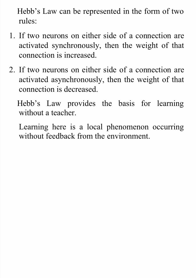
Hebb’s Law can be represented in the form of two

rules:

1. If two neurons on either side of a connection areactivated synchronously, then the weight of that

connection is increased.

2. If two neurons on either side of a connection areactivated asynchronously, then the weight of that

connection is decreased.

Hebb’s Law provides the basis for learningwithout a teacher.

Learning here is a local phenomenon occurring

without feedback from the environment.



Hebbian learning in a neural network

i j

I n p u t S i g n a l s

O u t p u t S i g n a l s



Using Hebb’s Law we can express the adjustment

applied to the weight w ij at iteration p in the

following form:

As a special case, we can represent Hebb’s Law as

follows:

wherea

is the learning rate parameter.This equation is referred to as the activity product

rule.

][ )(),()( p x py F pw i j ij

)()()( p x p y pw i jij a



• Hebbian learning implies that weights can only

increase.

• To resolve this problem, we might impose a limiton the growth of synaptic weights.

• It can be done by introducing a non-linear

forgetting factor into Hebb’s Law:

where j is the forgetting factor.Forgetting factor usually falls in the interval between 0 and 1,

typically between 0.01 and 0.1, to allow only a little

“forgetting” while limiting the weight growth.

)()()()()( pw py p x py pw ij j i j ij j-a



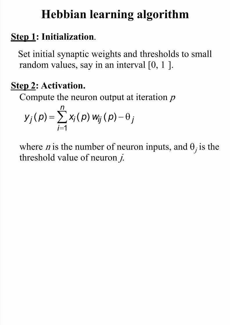
Step 1: Initialization. Set initial synaptic weights and thresholds to smallrandom values, say in an interval [0, 1 ].

Step 2: Activation. Compute the neuron output at iteration p

where n is the number of neuron inputs, and q j is the

threshold value of neuron j .

Hebbian learning algorithm

j

n

i ij i j pw p x py q-1 )()()(



Step 3: Learning.

Update the weights in the network:

where w ij ( p ) is the weight correction at iteration p .

The weight correction is determined by thegeneralised activity product rule:

Step 4: Iteration.Increase iteration p by one, go back to Step 2.

)()()1( pw pw pw ij ij ij

][ )()()()( pw p x py pw ij i j ij -j



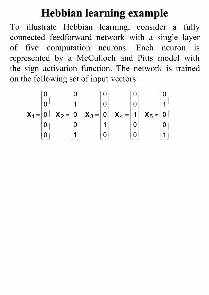
To illustrate Hebbian learning, consider a fully

connected feedforward network with a single layerof five computation neurons. Each neuron is

represented by a McCulloch and Pitts model with

the sign activation function. The network is trained

on the following set of input vectors:

Hebbian learning example

0

0

0

0

0

1X

1

0

0

1

0

2X

0

1

0

0

0

3X

0

0

1

0

0

4X

1

0

0

1

0

5X



Initial and final states of the network

Input layer

x 1 1

Output layer

2

1 y 1

y 2 x 2 2

x 3 3

x 4 4

x 5 5

4

3 y 3

y 4

5 y 5

1

0

0

0

1

1

0

0

0

1

Input layer

x 1

Output layer

2

1 y 1

y 2 x 2

x 3

x 4

x

4

3 y 3

y 4

5 y 5

1

0

0

0

1

0

0

1

0

1

2

5



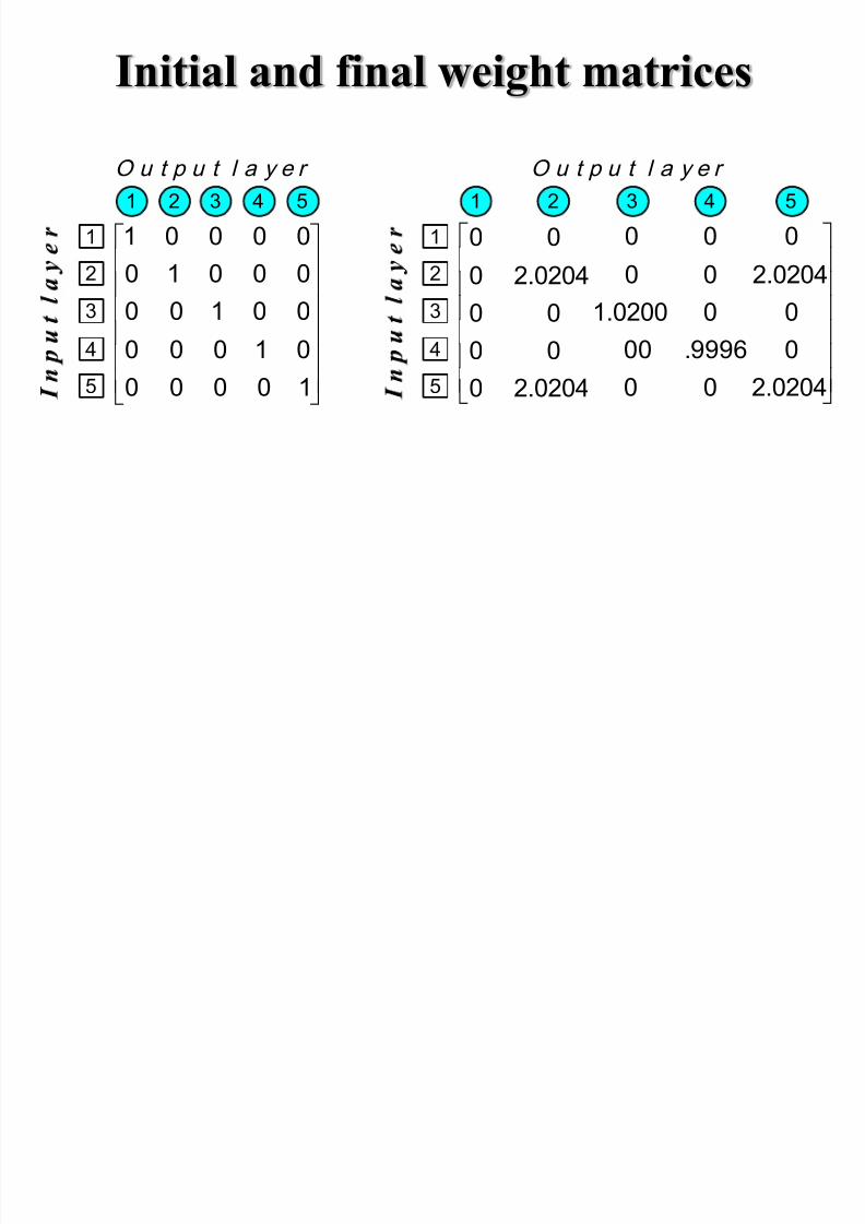
Initial and final weight matrices

O u t p u t l a y e r

10000

01000

00100

00010

00001

21 43 5

1

2

3

4

5

O u t p u t l a y e r

0

0

0

0

0

1 2 3 4 5

1

2

3

4

5

0

0

2.0204

0

2.0204

1.0200

0

0

0

00 .9996

0

0

0

0

0

0

2.0204

0

2.0204



A test input vector, or probe, is defined as

When this probe is presented to the network, weobtain:

1

0

0

0

1

X

-

1

0

0

1

0

0737.0

9478.0

0907.0

2661.0

4940.0

1

0

0

0

1

2.0204002.02040

00.9996000

001.020000

2.0204002.02040

00000

sign Y



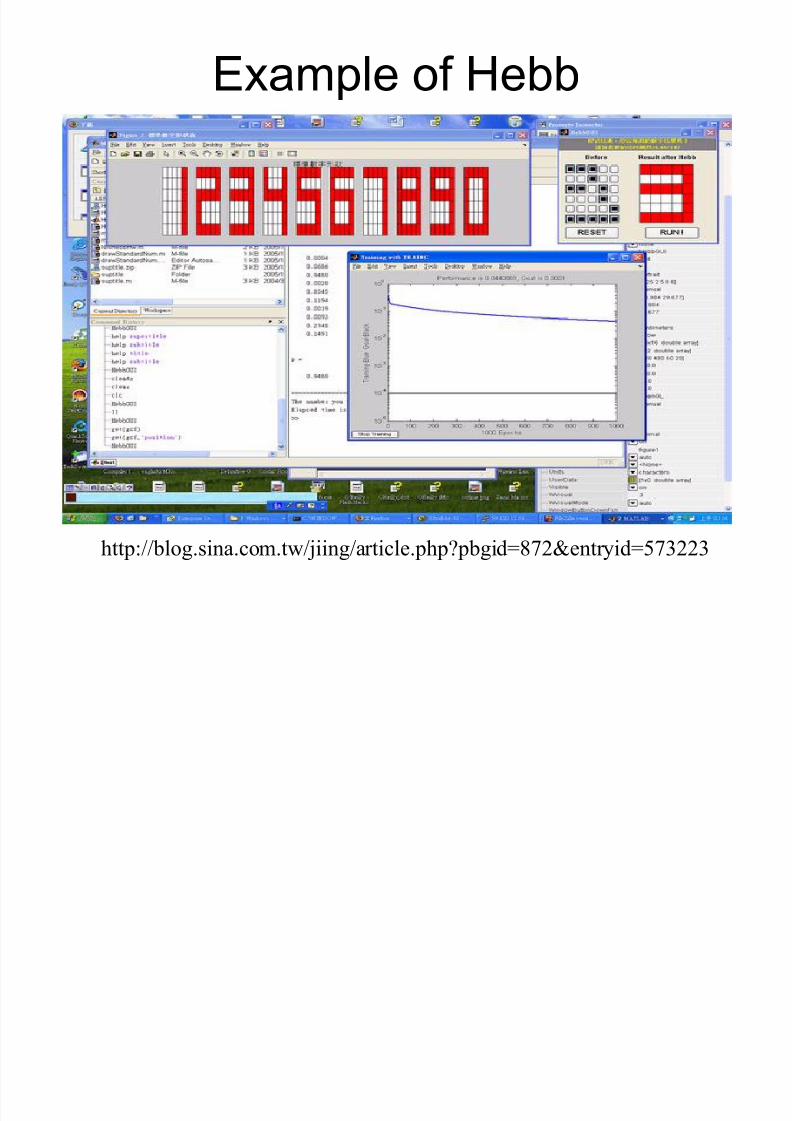
Example of Hebb

http://blog.sina.com.tw/jiing/article.php?pbgid=872&entryid=573223



In competitive learning, neurons compete among

themselves to be activateda.

While in Hebbian learning, several output neurons

can be activated simultaneously, in competitive

learning, only a single output neuron is active at

any time.

The output neuron that wins the “competition” is

called the winner-takes-all neuron.

Competitive learning



The basic idea of competitive learning was

introduced in the early 1970s. In the late 1980s, Teuvo Kohonen introduced a

special class of artificial neural networks called

self-organising feature maps. These maps are based on competitive learning.



Our brain is dominated by the cerebral cortex, a

very complex structure of billions of neurons and

hundreds of billions of synapses. The cortex

includes areas that are responsible for different

human activities (motor, visual, auditory,somatosensory, etc.), and associated with different

sensory inputs. We can say that each sensory

input is mapped into a corresponding area of the

cerebral cortex. The cortex is a self-organising

computational map in the human brain.

What is a self-organising feature map?



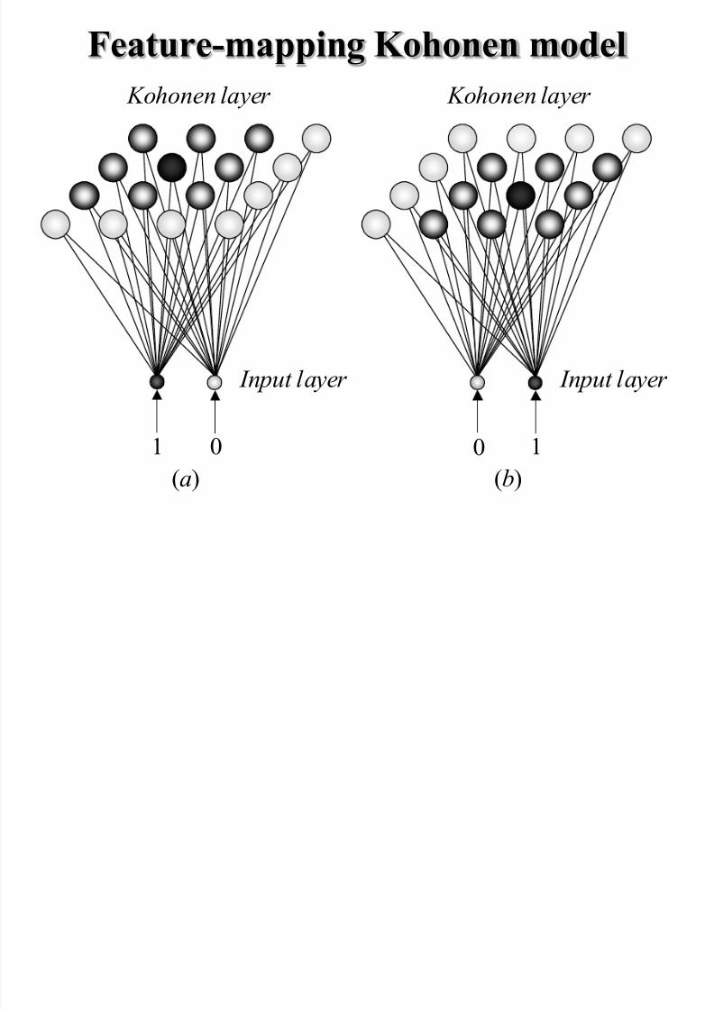
Feature-mapping Kohonen model

Input layer

Kohonen layer

(a)

Input layer

Kohonen layer

1 1

(b)

00



The Kohonen network

The Kohonen model provides a topologicalmapping. It places a fixed number of input

patterns from the input layer into a higher-

dimensional output or Kohonen layer.

Training in the Kohonen network begins with the

winner’s neighbourhood of a fairly large size.

Then, as training proceeds, the neighbourhood size

gradually decreases.



Architecture of the Kohonen Network

Input

layer

x1

x2

Output

layer

y

y2

1

y3



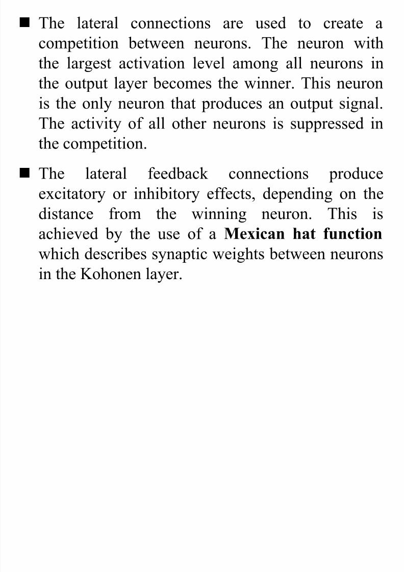
The lateral connections are used to create a

competition between neurons. The neuron with

the largest activation level among all neurons in

the output layer becomes the winner. This neuron

is the only neuron that produces an output signal.

The activity of all other neurons is suppressed in

the competition.

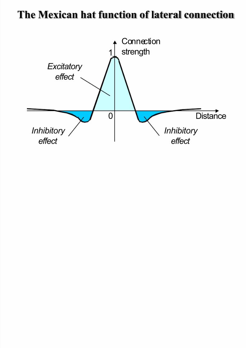
The lateral feedback connections produce

excitatory or inhibitory effects, depending on the

distance from the winning neuron. This isachieved by the use of a Mexican hat function

which describes synaptic weights between neurons

in the Kohonen layer.



The Mexican hat function of lateral connection

Connectionstrength

Distance

Excitatory

effect

Inhibitory effect

Inhibitory effect

0

1



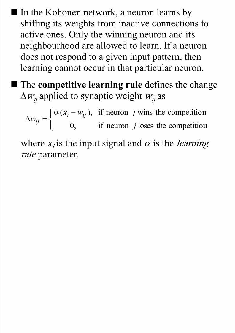
In the Kohonen network, a neuron learns byshifting its weights from inactive connections toactive ones. Only the winning neuron and its

neighbourhood are allowed to learn. If a neurondoes not respond to a given input pattern, thenlearning cannot occur in that particular neuron.

The competitive learning rule defines the changew ij applied to synaptic weight w ij as

where x i is the input signal and a is the learningrate parameter.

-

ncompetitiothelosesneuronif ,0

ncompetitiothewinsneuronif ),(

j

jw xw

iji

ij

a



The overall effect of the competitive learning rule

resides in moving the synaptic weight vector W j of

the winning neuron j towards the input pattern X.

The matching criterion is equivalent to the

minimum Euclidean distance between vectors.

The Euclidean distance between a pair of n -by-1

vectors X and W j is defined by

where x i and w ij are the i th elements of the vectors

X and W j , respectively.

2/1

1

2)(

--

n

i ij i j w x d WX



To identify the winning neuron, j X, that best

matches the input vector X, we may apply thefollowing condition:

where m is the number of neurons in the Kohonen

layer.

, j

j

min j WXX - j = 1, 2, . . .,m



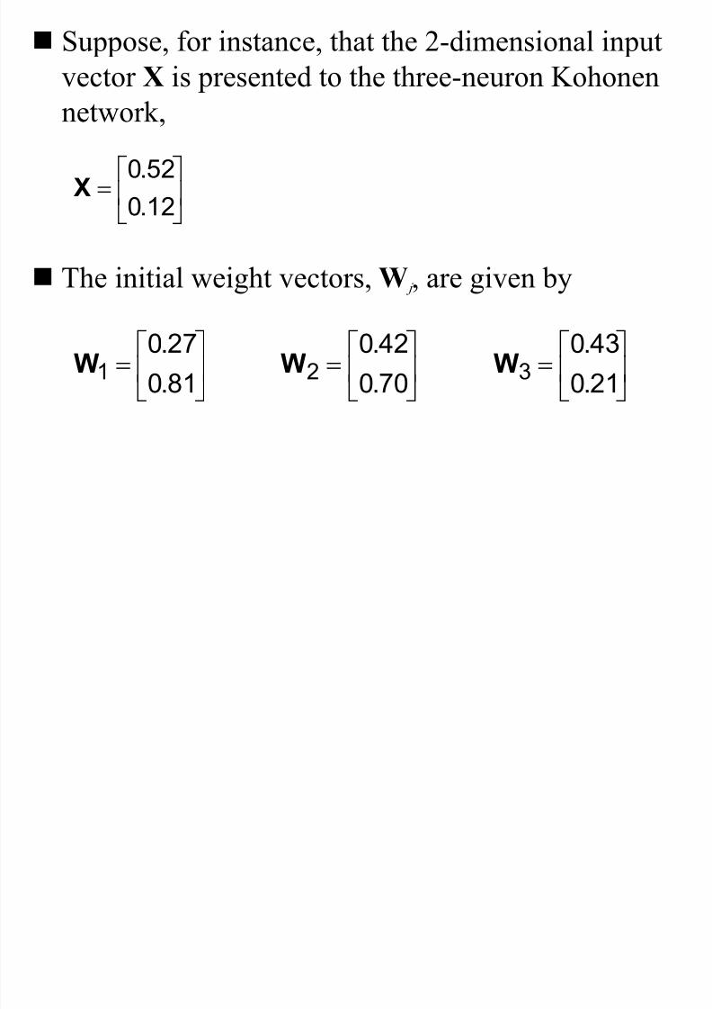
Suppose, for instance, that the 2-dimensional input

vector X is presented to the three-neuron Kohonen

network,

The initial weight vectors, W j , are given by

12.0

52.0X

81.0

27.0

1W

70.0

42.0

2W

21.0

43.0

3W



We find the winning (best-matching) neuron j X

using the minimum-distance Euclidean criterion:

Neuron 3 is the winner and its weight vector W3 is

updated according to the competitive learning rule.

2212

21111 )()( w x w x d -- 73.0)81.012.0()27.052.0( 22 --

2222

21212 )()( w x w x d -- 59.0)70.012.0()42.052.0(

22 --

2

232

2

1313 )()( w x w x d -- 13.0)21.012.0()43.052.0(

22

--

0.01)43.052.0(1.0)( 13113 -- w x w

0.01)21.012.0(1.0)( 23223 --- w x w



The updated weight vector W3 at iteration ( p + 1)

is determined as:

The weight vector W3 of the wining neuron 3

becomes closer to the input vector X with each

iteration.

-

20.0

44.0

01.0

0.01

21.0

43.0)()()1( 333 p p p WWW



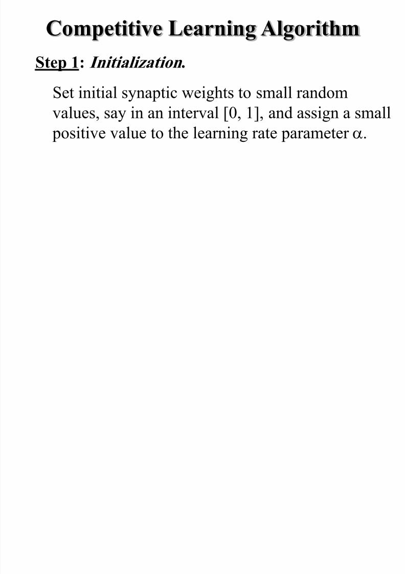
Competitive Learning Algorithm

Set initial synaptic weights to small random

values, say in an interval [0, 1], and assign a small

positive value to the learning rate parameter a.

Step 1: Initialization .



Activate the Kohonen network by applying the

input vector X, and find the winner-takes-all (bestmatching) neuron j X at iteration p , using the

minimum-distance Euclidean criterion

where n is the number of neurons in the input

layer, and m is the number of neurons in the

Kohonen layer.

,)()()(

2/1

1

2][

--

n

i ij i j

j pw x pmin p j WXX

j = 1, 2, . . .,m

Step 2: Activation and Similarity Matching .



Update the synaptic weights

where w ij ( p ) is the weight correction at iteration p .

The weight correction is determined by the

competitive learning rule:

where a is the learning rate parameter, and L j ( p ) is

the neighbourhood function centred around the

winner-takes-all neuron j X at iteration p .

)()()1( pw pw pw ij ij ij

L

L-

)(,0

)(,)()(

][

p j

p j pw x pw

j

j ij i ij

Step 3: Learning .



Increase iteration p by one, go back to Step 2 and

continue until the minimum-distance Euclideancriterion is satisfied, or no noticeable changes

occur in the feature map.

Step 4: Iteration .



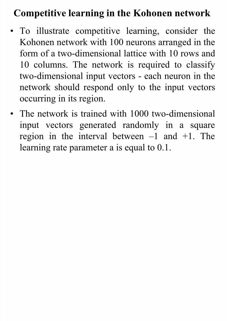
Competitive learning in the Kohonen network

• To illustrate competitive learning, consider the

Kohonen network with 100 neurons arranged in theform of a two-dimensional lattice with 10 rows and

10 columns. The network is required to classify

two-dimensional input vectors - each neuron in thenetwork should respond only to the input vectors

occurring in its region.

• The network is trained with 1000 two-dimensional

input vectors generated randomly in a square

region in the interval between – 1 and +1. The

learning rate parameter a is equal to 0.1.

i i i



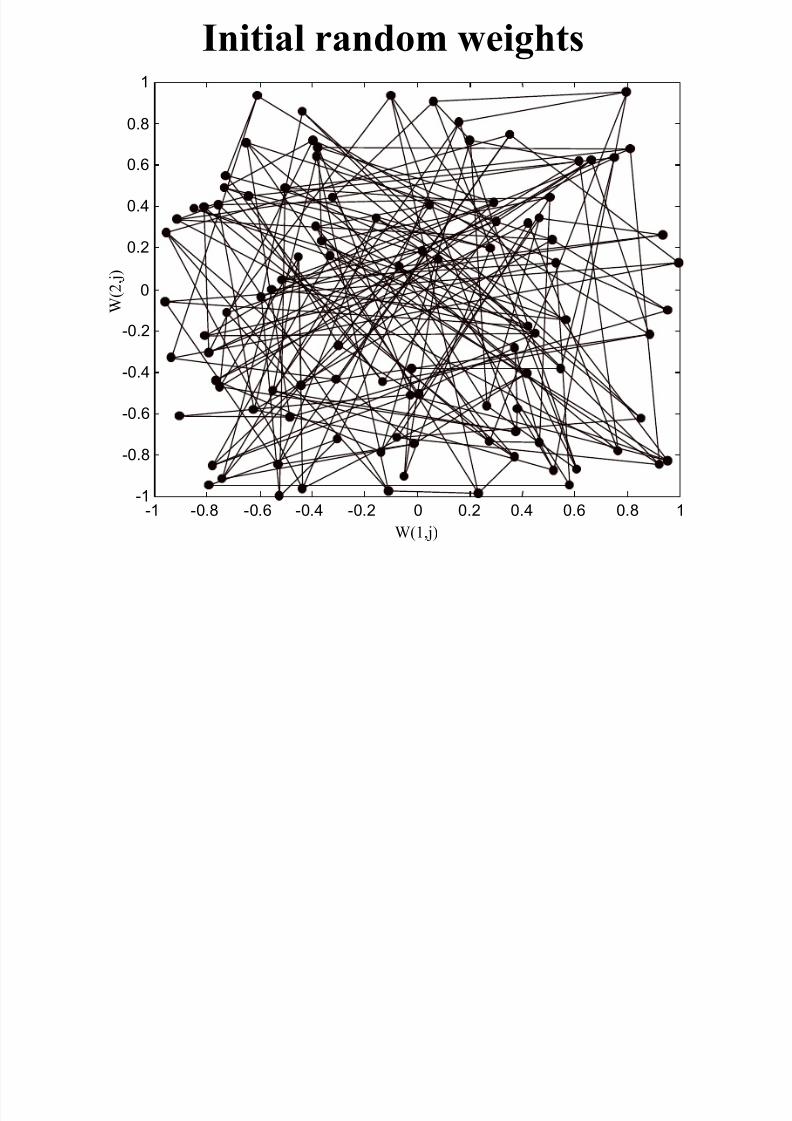
Initial random weights

-0.8 -0.6 -0.4 -0.2 0 0.2 0.4 0.6 0.8 1-1-1

-0.8

-0.6

-0.4

-0.2

0

0.2

0.4

0.6

0.8

1

W ( 2 , j )

W(1,j)

N k f 100 i i



Network after 100 iterations

-0.8 -0.6 -0.4 -0.2 0 0.2 0.4 0.6 0.8-1-1

-0.8

-0.6

-0.4

-0.2

0

0.2

0.4

0.6

0.8

1

1

W ( 2 , j )

W(1,j)

N k f 1000 i i



Network after 1000 iterations

-0.8 -0.6 -0.4 -0.2 0 0.2 0.4 0.6 0.8-1-1

-0.8

-0.6

-0.4

-0.2

0

0.2

0.4

0.6

0.8

1

1

W ( 2 , j )

W(1,j)

N t k ft 10 000 it ti



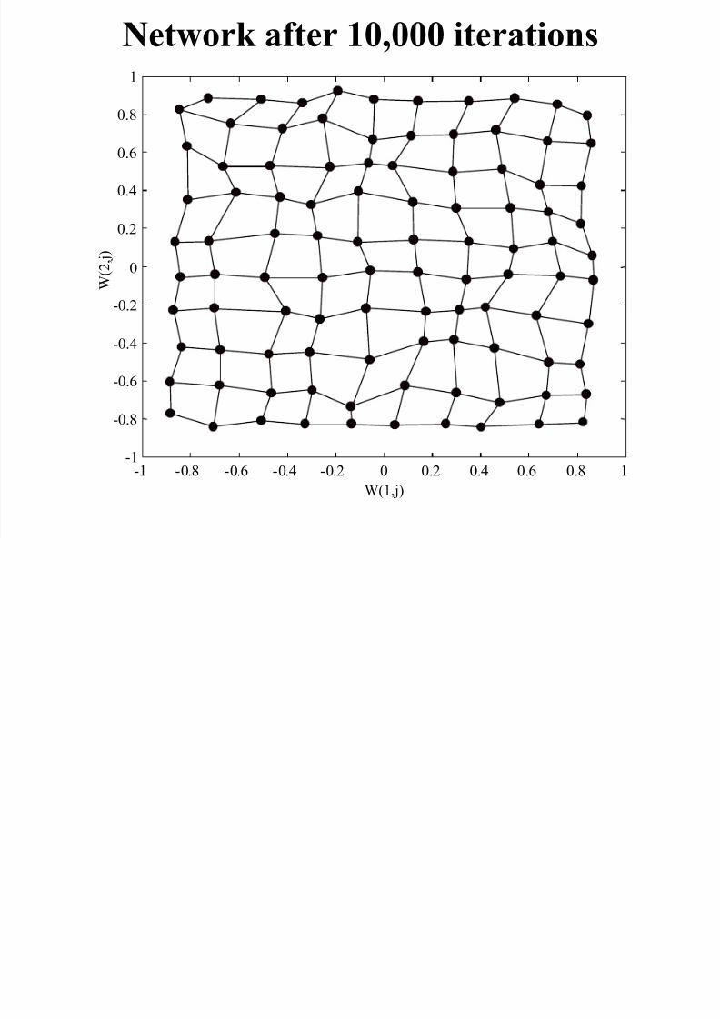
Network after 10,000 iterations

-0.8 -0.6 -0.4 -0.2 0 0.2 0.4 0.6 0.8-1-1

-0.8

-0.6

-0.4

-0.2

0

0.2

0.4

0.6

0.8

1

1

W ( 2 , j )

W(1,j)

8. artificial neural networks-unsupervised learning.pdf

Documents