8 correlation profiles and motifs in complex networks

BNL-71995-2004-BC

8 Correlation Profiles and Motifs in Complex Networks

Sergei Maslov, Kim Sneppen, aid Uri Alon

8.1 Introduction Networks have recently emerged as a unifying theme in complex systems research [l]. It is in fact no coincidence that networks and complexity are so heavily intertwined. Any future definition of a complex system should reflect the fact that such systems consist of many mutually interacting components. These components are far from being identical as say electrons in systems studied by condensed matter physics. In a truly coniplex system each of them has a unique identity allowing one to separate it from the others. The very first question one may ask about such a system is which other components a given component interacts with? This information systemwide can be visualized as a graph, whose nodes correspond to individual components of the complex system in question and edges to their mutual interactions. Such a network can be thought of as a backbone of the complex system. Of course, system’s dynamics depends not only on the topology of an underlying network but also on the exact form of interaction of components with each other, which can be very different in various complex systems. However, the underlying network may contain clues about the basic design principles andor evolutionary history of the complex system in question. The goal of this article is to provide readers with a set of useful tools that would help to decide which features of a coniplex network are there by pure chance alone, and which of them were possibly designed or evolved to their present state.

Living organisms provide us with a paradigm for a complex system. Therefore, it should not be surprising that in biology networks appear on many different levels. All biochemi- cal processes taking place in a single cell constitute its metabolic network, where nodes are individual metabolites, and edges are metabolic reactions converting them to each other. Vir- tually every one of these reactions is catalyzed by an enzyme and the specificity of its catalytic function is ensured by the key and lock principle of its physical interaction with the substrate. Often the functional enzyme is formed by several mutually interacting proteins. Thus the structure of the metabolic network is shaped by the network of physical interactions of cell’s proteins with their substrates and each other. Another way in which the network of physical interactions contributes to the complex dynamics of a living cell is through regulation of ac- tivity of individual proteins e.g. by phosphorylation or allosteric regulation. This constitutes a major mechanism for propagation of various biocheinical signals in the cell. Hence a more complete version of the physical interaction network in addition to substrates and proteins should also include all of their functionally modified forms. The prolduction and degradation of each of the proteins in the physical interaction network in turn is controlled by the regulatory network of the cell. In Fig. 8.1 we show a part of such network in the bacterium

S. I Iiztrodzictiori 171

Escherichia coli (E.coli) corresponding to positive or negative transcriptional regulation of its proteins by transcription factors. More generally regulatory network in the cell in addition to transcriptional regulation includes translational regulation, RNA editing, specific targeting of individual proteins for degradation, etc. On yet higher level individual cells of a multicellular organism exchange signals with each other. This gives rise to several new networks such as e.g. nervous, hormonal, and iminune systems of an animal. The inter-cellular signaling network stages the development of a multicellular organism of a given species from the fertilized egg. Finally. on even larger scale interactions between individual species form the food web of an ecosystem.

By no means complex networks are unique to living organisms: in fact they lie at the foundation of an increasing number of artificial systems. The most prominent example of this is the Internet and the World Wide Web (WWW) being the “hardware” and the “software” of the network of communications between computers. While the Internet is formed by “physical” connections between constituent computers, or on a more coarse-grained scale, between so-called Autonomous Systems (AS), which are large domains of computers managed by the same organization such as e.g a university, or a business enterprise. The World Wide Web, on the other hand, is a much larger network whose nodes are individual webpages, and directed edges are links between them.

Networks are also ubiquitous in systems studied by social sciences. To name just a few, scientists are connected by a network of collaborations defined as co-authorship of scientific articles, while articles themselves are linked through a directed network of citations. Ex- amples of networks in economics include that of customers and their choices of products, or economies of individual countries connected by the volume of direct foreign investments. This last example illustrates one important notion about complex networks: in some cases it appears that every component of a complex system is connected to every other component, which makes the concept of a network useless. Indeed, in this case the network is just a fully connected graph, which contains no information about the complexity of the underlying system. However, a meaningful network can be constructed in this case if one chooses to include only interactions stronger than a certain threshold, which has to be selected to maximize the information content of the resulting graph. For interacting economies that corresponds to including edges only for the strongest coupled pairs of countries, while for physical interaction networks in biological systems - for pairs of molecules with the binding constant above a certain threshold.

The above mentioned complex networks in biological, technological, and social systems for the most part lack the top-down design. Instead they grow and evolve as a result of the bottom-up stochastic dynamics of their individual nodes. It makes an Erdos-RCnyi (ER) random network [3] the first null model to which topological properties of these networks can be compared. An interesting unifying feature of many complex networks that clearly distin- guishes them from ER random networks is an extremely broad distribution of connectivities (defined as the number of immediate neighbors) of individual nodes [4]. While the major- ity of nodes in such a network are each connected to just a handhl of neighbors, there exist some nodes, which will be referred to as “hubs”, that have a disproportionately large number of interaction partners. The connectivity of the highest connected hub is usually several orders of magnitude larger than the average connectivity of the network. This property stands in sharp contrast with ER networks, in which connectivities of individual nodes are Poisson-

172 8 Correlatioii ProJires arid Motgs in Complex Nehvorh-s

Figure 8.1: The transcription regulatory netwoi

@% Pajek

of E.coli. Nodes in this network represent operons - (groups of genes transcribed onto a single mRNA) and arrows (edges) - direct transcriptional regulation of a protein encoded in the downstream operon by a regulatory protein encoded in the upstream operon. Red and green arrows refer to respectively negative and positive regulations in a living E.co1i cell. In the present text we discuss how one can extract characteristic topological properties of networks such as the one shown here. The network was displayed using the Pajek software [2].

8.1 Znt~oduction 173

distributed and thus the number of nodes with a connectivity significantly above average is negligibly small. Often the connectivity distribution in complex networks can be approximated by a scale-free power law form [4]. Prominent examples of this are the Internet [5] and the WWW [6], where in the last case the power law extends for up to four orders of magnitude. Among biological networks histograms of node connectivities in metabolic [7] and protein interaction [8] networks can be reasonably approximated by scale-free distributions extending for about two orders of magnitude.

The set of connectivities of individual nodes is an example of a low-level topological property of a network. While it answers the question about how many neighbors a given node has, it gives no information about the identity of those neighbors. It is clear that most of non- trivial properties of networks are defined at a higher level in the exact pattern of connections of nodes to each other. However, such multi-node connectivity patterns are rather difficult to quantify and measure. By just looking at many complex networks one gets the impression that their components are linked to each other in a completely haphazard way. One may wonder which connectivity patterns are indeed random, while which arose due to evolution or fundamental design principles and limitations? Such non-random features can be used to identify a given complex network and better understand the underlying complex system.

In this work we describe a universal recipe for how such information can be extracted. To this end we first construct a proper randomized version (null model) of a given network. As was pointed out by Newman and collaborators [9], broad distributions of connectivities observed in most real complex networks indicate that the connectivity is an important individual characteristic of their nodes and as such it should be preserved in any meaningful random counterpart. In addition to connectivities of its nodes one may choose to preserve some other low-level topological properties of the network. Any higher level topological proplerty, such as e.g. the total number of edges connecting pairs of nodes with given connectivities, the number of loops of a certain type, the number and sizes of components, the diameter of the network, can then be measured in the real complex network and separately in an ensemble of its randomized versions. Dealing with an ensemble allows one to put error bars on any quantity measured in the randomized network. One then concentrates only on those topological properties of the complex network that significantly deviate from the null model, and, therefore, are likely to reflect its design principles and/or evolutionary history.

The idea of comparing topological properties of a network to its randomized counterpart is not new. For example, in [lo] the level of clustering in some real world networks was compared to its value in ER random networks with the same number of edges and nodes. In the field of sociology there exists a rich history of testing hypotheses about social networks by comparison to randomized null-model networks [ 1 I]. A more recent twist on this idea was put in Ref. [9 ] . Authors of this work derived a number of useful analytical results for random networks with an arbitraiy distribution of connectivities and compared certain topological properties of a number of real-life complex networks to these analytical expressions. In Ref. [ 121 it was demonstrated that when constructing a random network with a broad distribution of connectivities it is important to take into account the constraint of having no multiple edges between the same pair of nodes, This constraint applicable to most real-life complex networks modifies topological properties of their random counterparts, especially around their highly connected (hub) nodes. One may also select to conserve some other low-level topological properties in addition to connectivities of individual nodes [12]. In the absence of analytical

174 8 Corr.elation Profiles and Mot$s in Complex Networks

results in this case one has to resort to numerical simulation of such randomized networks Basic algorithms generating an ensemble of such random networks were applied to studies of complex networks in [13, 14, 121. Earlier on these algorithms were .actively studied in mathematical literature [15]. In these works a number of important results concerning their ergodicity were rigorously proven.

The plan of this review is as follows: In the next section we introduce the local rewiring algorithm for generation of an ensemble of randomized networks [15, 13, 121 and compare it with global rewiring algorithms studied in [16. 91. We also propose several modifications of this algorithm, which in addition to node connectivities conserve some other low-level topological properties of the complex network in question [12]. In the section 3 we use these random ensembles to measure correlation profiles of several complex networks, namely those of physical interactions and transcriptional regulation between proteins in yeast Succ!zar.ornyces cemvisiae [ 131, and that of the Internet defined on the level of Autonomous Systems (AS) [ 121. In the section 4 the comparison to a randomized network reveals the set of ubiquitous network motifs in the genetic regulatory network of Escherichia coli bacterium [ 141. The potential meaning of these empirically detected elements of design is discussed in the last section. The set of MATLAB numerical algorithms used to generate some of the results described in this work can be found at [ 171.

8.2 Randomization algorithm: Constructing the proper null model

One may generate a random version of a given network using various algorithms. They differ from each other bywhich low-level topological features of the original network are preserved in its randomized counterpart. Below are the first three representatives of such randomization algorithms listed in the order of increasing number of constraints:

1. Randomly rewire all edges in the network. This algorithm only conserves the uvwuge connectivity of all nodes in the network.

2. Randomly rewire edges in the network while preserving the number of edges emanating from each individual node (node’s connectivity). This algorithm conserves all “single- node” topological properties of a network, while completely randomizes multi-node connection patterns. In a directed network one may rewire edges in such a way that both the number of outgoing and incoming edges are separately conserved for each node.

3. When nodes in a network are divided into several mutually exclusive subgroups one may rewire its edges in such a way that the total number of neighbors from each of these subgroups is separately conserved for every node. This algorithm may prove use l l if some subgroups are known to preferentially connect to some other subgroups and one wants to preserve this preferential linking in a randomized network.

The first rewiring scheme from the list above irrespective of the original form of this distribution generates an Erdos-Rhyi (ER) random network characterized by a narrow Poisson distribution p ( k ) = (k)k exp(-(k))/k! of node connectivities k. As both percolation properties and the abundance of most topological patterns in a network are very sensitive to the

S.2 Raiidoniizatioii algoritliiii: Coiistructing the proper iiuII model 175

exact form of the distribution of connectivities [18, 91, they would be dramatically modified as a result of the randomization algorithm 1. A much more informative comparison is to a randomized network generated by algorithms 2-3, where connectivities of individual nodes (and hence their distribution) are strictly conserved.

The rewiring algorithm giving rise to such random network was proposed in [15, 131. In its most general formulation (for a directed network whose nodes are divided into several subgroups) it consists of multiple repetition of the following switch move (rewiring step) (see illustration in Fig. 8.2):

Randomly select a pair of directed edges A+B and C-D where A and C belong to the same subgroup (marked blue in Fig. 8.2), and B and D belong to the same subgroup (marked red in Fig. 8.2). The two edges are then rewired in such a way that A becomes connected to D, while C to B, provided that none of these edges already exist in the network, in which case the rewiring step is aborted and a new pair of edges is selected.

A /f \ D

/

switch partners

A

Figure 8.2: One step of the random local rewiring algorithm. A pair of directed edges A+B and C+D such that nodes A and C belong to the same subgroup (marked blue), and B and D both belong to another subgroup (marked red) are selected. The two edges are then rewired in such a way that A becomes connected to D, while C to B, provided that none of these edges already exist in the network, in which case the rewiring step is aborted and a new pair of edges is selected. An independent random network is obtained when the network is rewired by the above local switch a large number of times, say several times in excess of the total number of edges in the system. The above rewiring algoritlim c,onserves both the in- and out- connectivity of each individual node as well as the exact distribution of its interaction partners among subgroups of nodes.

The last restriction prevents the appearance of multiple edges connecting the same pair of nodes. A repeated application of the above rewiring step leads to a randomized version of the original network. The set of MATLAB programs generating such a randomized version of any complex network can be downloaded from [17].

176 8 Correlatiun Projles and Motij5 in Complex NebvurJis

A number of nice analytical results for random networks with an arbitrary (in general non-Poisson) probability distribution of connectivities were recently reported in [ 18,9]. Also, in Refs. [16, 91 a “stub reconnecting” numerical algorithm allowing one to construct such networks was proposed. The basic idea of this algorithm was to first generate the set of connectivities ki for every node in the system, and create ki “edge stubs“ sticking out of every node, which are not yet connected to other nodes. A random network is then generated by randomly picking two such edge stubs and joining them together to form an edge between the two nodes they emanate from. As this process goes on the number of disconnected stubs diminishes until finally all stubs are used up.

The stub reconnecting algorithm explicitly allows for multiple edges to form between the same pair of nodes. On the other hand, the construction principles o f complex networks discussed in this paper prohibit the appearance of such multiple edges, and hence they should not be allowed in their random counterparts as well. If one explicitly forbids the formation of multiple edges during the stub reconnecting algorithm [ 16, 91, for sufficiently broad distribution of node connectivities the algorithm would normally get stuck in a L‘frozen’’ configuration in which all nodes with remaining unconnected stubs are already connected to each other. The probability to reach such a frozen configuration increases with both the size and the fraction of highly connected nodes in the network. In this case it becomes computationally impossible to avoid double edges by aborting and restarting the algorithm every time a frozen configuration is reached. We would also like to point out that the set of analytical results obtained in [ 18,9] apply to an ensemble of random networks generated by the stub reconnecting algorithm in which multiple edges are allowed. Therefore, they have to be modified for an ensemble of random networks in which such edges are forbidden.

The above mentioned limitations of the stub reconnecting algorithm forced us to use the local rewiring algorithm [ 15, 13, 121 described above. Instead of completely deconstnicting a given complex network and then creating the corresponding random network de izovo this algorithm modifies it through multiple simple local rearrangements and hence avoids frozen configurations. Later on in this section we will show how the basic rules of our local rewiring algorithm can be recursively modified to analyze patterns present at higher levels of network architecture, while maintaining other established low-level topological properties of the complex network in addition to connectivities of its nodes.

The difference in frequencies of appearance of any particular topological pattern j in a given complex network and its properly randomized counterpart can be quantified by the following set of con’elation profiles. In the first profile one computes the ratio

- where N ( j ) is the number of times the pattern j is seen in the real network, and NT(j) is the average number of occurrences of the pattern in an ensemble of random networks generated by the appropriate null model. Patterns selected by design or evolution of the complex network in question would manifest themselves by R(j ) > 1, while suppressed patterns correspond to R(j ) < 1. While R(j ) determines the magnitude of the suppressiodenhancement it tells

5.2 Rnndoiiiizatioii algorithm: Corzstriictiizg the proper null model 177

nothing about the statistical significance of the effect. This latter quantity is given by the Z-score of the deviation defined as

where uT ( j ) is the standard deviation of N,. ( j ) measured in a sufficiently large ensemble of randomized networks.

Alternatively the statistical significance of the difference between real and randomized networks can be quantified in terms of its P-value. The P-value is defined as the probability that the number of patterns N, ( j ) in a randomized network is larger or equal (or smaller or equal in case when N ( j ) < N T ( j ) ) than N ( j ) . For patterns that are highly statistically significant it is often impossible to directly evaluate the P-value in a reasonable number of realizations of random networks. In this case one reports an upper bound on such a P-value given by the inverse size of the ensemble studied numerically. If one can verify that N, is a Gaussian-distributed random variable the Z-score can be easily converted to the P-value.

-

Examples of patterns discussed in this work include:

0 Correlations between connectivities of neighboring nodes quantified as N(K0, K1) - the number of edges connecting nodes of connectivity IC0 to those of connectivity IC1 [13, 121;

0 The number of small network motifs [I41 such as e.g. the triangular loop (Fig. 8.3A), or

In case of more complex topological patterns like the double triangle in Fig. 8.3B the calculation of R and Z becomes somewhat more involved. Indeed since this pattern contains two simple triangles and a square among its sub-patterns, its statistical over- or under- repre- sentation in the real network may be caused simply by over- or under- representation of these more elementary sub-patterns. One strategy is to deal with this problem recursively and ana- lytically [ 141. In this case one has to start computing 2 and R from the simplest “irreducible” patterns and gradually work it up toward more complicated composite patterns, each time renornializing out trivial “reducible” correlations. Another strategy numerically deteiinines the statistical significance of a given high-level topological motif [12]. To this end one first generates an ensemble of random networks that have both the same set of connectivities and the same number of low-level motifs (such as e.g. triangle loops) as the original network. This can be done in several different ways:

1. One may consider only those local rewiring steps that strictly preserve both node connectivities and the number of sub-motifs. One example of such specific move is shown in Fig. 8.4, which conserves both node connectivities and the total number of simple triangular loops.

the double triangle (Fig. 8.3B).

2. One may employ the switch move in Fig. 8.2, without constraint, but then limit the ensemble generated by the simple rewiring algorithm to include only networks which by accident have the observed number of sub-motifs. In most cases this algorithm is

178 8 Correlation Projles and Motifs in Coinplex Networks

prohibitively numerically expensive, in particular when the sub-motifs in the real network are hugely overrepresented on underrepresented relative to a typical random network.

3. A way to remedy the numerical inefficiency of the previous algorithm is to use biased sampling, which favors the correct number of sub-motifs. This can be done by supple- menting the simple switch move with a Metropolis acceptancehrejection criterion based on an artificial energy function Hj that favors the same number of sub-motifs j that was observed in the real network [12]:

That is to say for a given temperature T, the algorithm accepts any local rewiring step that lowers the energy Hj or leaves it unchanged, while those steps that lead to a A H increase in Hj are accepted with a probability exp(-AHIT). The temperature should be selected low enough to favor the desired number of low-level sub-motifs j yet high enough to ensure an ergodic sampling of the phase space. Obviously the T = 0 version of this algorithm is equivalent to the algorithm #I.

The Metropolis algorithm #3 can be easily extended to take care of several independent sub-motifs by using the composite energy function H = Hj. Such sampling of networks has the advantages of being simple to implement and generalizes easily to several sub-patterns. When counting the statistics one can limit the ensemble to include only the random networks that have exactly the same number of sub-motifs as the original complex network.

Figure 8.3: Example of motifs: (A) a simple triangle whose abundance quantifies the level of clustering in the network. (B) a somewhat more complex pattern. It contains two triangles and a square among its sub-patterns.

S.3 Correlation profiles: East inoleciilar networks and the Internet 179

A B C \ L A B C

Figure 8.4: The local rewiring step shown in the panel A is allowed since it preserves the total number of triangles in the network, while that in the panel B is forbidden since it decreases the number of triangles by one. In the Metropolis algorithm both moves would be allowed albeit with different probabilities: move in panel B would be accepted with a lower probability due to the increase in the energy function (5.3).

8.3 Correlation profiles: Yeast molecular networks and the Internet

Methods described in the previous section allow us to define and measure the correlation pro$le of a complex network. The correlation profile quantifies correlations between connectivities of neighboring nodes in the network. We have applied these numerical tools to two levels of molecular networks operating in yeast Saccharonzyces cerevisiae, which at present is perhaps the best characterized biological model organism:

The protein interaction network used in this work consists of 4475 physical interactions between 3279 yeast proteins as measured in the most comprehensive high-throughput yeast two-hybrid screen [19]. To answer the question if proteins A and B interact with each other the two-hybrid experimental technique uses a pair of artificially prepared hybrid proteins Ab and BP, which are referred to as the bait and the prey hybrid correspondingly. In order to better visualize the protein interaction network in Fig. 8.5 we plotted a small part of it using the software package Pajek developed by Vladimir Batagelj and Andrej Mrvar [2]. The subset used in this figure consists of all proteins known to be localized in the yeast nucleus [20] and to interact with at least one other nuclear protein in the full set of Ref. [ 191.

2. The most general definition of the reguulatory network operating in a living cell includes all cases when production or degradation of one of its proteins is directly controlled by another. Edges of this network correspond to transcription and translational regulation, RNA editing, specific targeting of individual proteins for degradation, etc. The YPD

180 S Correlation Profiles and Motgs in Coiipla Networks

Figure 8.5: Network of physical interactions between nuclear proteins in yeast. Here we show the subset of the yeast protein interaction network reported in the full set of Ref. [19]. The subset consists of 318 interactions among 329 proteins, which are known to be localized in the yeast nucleus [20], and to interact with at least one other nuclear protein [19]. Note that most neighbors of highly connected nodes have rather low connectivity. This feature will be later quantified in the correlation profile of this network (Figs 8.7, 8.9). Nodes are color coded according to how essential they are for the survival of yeast cells under laboratory conditions [20]. Green nodes correspond to viable and red ones to non-viable null-mutants lacking the corresponding protein.

database [20] contains 1750 such regulations among 848 yeast proteins. To narrow down the range of possible regulatory mechanisms and make the network more homogeneous we have constructed correlation profiles of the transcription regulatory network, which is the subset of the general regulatory network formed by all positive and negative direct transcription regulations. This network shown in Fig. 8.6 consists of 1289 (1047 positive

8.3 Correlation projles: Yeast nzolecular iietworh and the Internet 181

Pajek

Figure 8.6: Transcription regulatory network in yeast. Apart from an overall apparent lack of modularity, one notices several striking features related to hub proteins that each regulate many other proteins: 1) they tend to avoid to regulate each other, 2) each hubs is either a predominantly positive regulator or a predominantly negative regulator, and 3) it is much more frequent for a protein to regulate many other proteins, than to be regulated by many. It is the first of these features, the separation of hubs from each other, that is quantified witlithe correlation profile of this network (Figs 8.8, 8.10.)

and 242 negative) regulations by 125 transcription factors [20] within the set of 682 proteins.

While the regulatory network is naturally directed, the network of physical interactions among proteins in principle lacks directionality. However, for poorly understood reasons all high-throughput two-hybrid experimental data [22, 191 defining pairs of physically interacting

182 8 Correlation Profies and Mot$ in Complex Networlcs

proteins have a significant asymmetry between baits and preys, with bait hybrids being more likely to be highly connected than their prey counterparts. This can be seen e.g. in the fact that the average connectivity of baits with at least one interaction partner is close to 3, whereas the same quantity measured for preys is only 1.8. Since each reported interaction involves exactly one bait and one prey protein, this asymmetry needs to be taken into account when selecting a proper “null” model for the interaction network. For this purpose in our randomization procedure we would treat the two-hybrid data as a directed network with an arrow on each edge pointing away from the bait hybrid towards the prey hybrid.

Randomized versions of these two molecular networks were constructed by randomly rewiring their directed edges, while preventing “unphysical” multiple connections between a given pair of nodes as described in the previous section. By construction this algorithm separately conserves the in- and out-connectivities of each node. Therefore, in a randomized

. version of the regulatory network each protein has the same numbers of regulators and regulated proteins as in the original network. Similarly, in a random counterpart of the interaction network numbers of interaction partners of the bait-hybrid and the prey-hybrid of every protein are individually conserved. The set of MATLAB programs for both the randomization and the correlation profile detection and visualization in any complex network are available at

The topological property of the network giving rise to its correlation profile is the number edges N( KO, K1) connecting pairs of nodes with connectivities KO and Kl. To find out if in a given complex network connectivities of interacting nodes are correlated, N(Ko,I(1) should be compared to its value N,(Ko, K1) .tAN,(Ko, K 1 ) in a randomized network, generated by the edge rewiring algorithm. When normalized by the total number of edges E, N(K0, K-1)

defines the joint probability distribution P(I<-0, K1) = N(K0, Kl)/E of connectivities of interacting nodes. Any correlations would manifest themselves as systematic deviations of the ratio

~ 7 1 .

R ( ~ ~ o , K 1 ) = WO,I~l)/PT(KO,I(1) (8.4)

Z(l(0, K1) = ( W C o , Kl) - PT(I(0, I ( 1 ) ) l f l T ( I ( O , K1) ,

from 1. Statistical significance of such deviations is quantified by their Z-score

(8.5)

where cr,(Ko,K1) = ANT(K0,K1)/N is the standard deviation of PT(Ko,K1) in an ensemble of randomized network.

Figs. 8.7 and 8.8 show the ratio R(K0, K1) as measured in yeast interaction and transcription regulatory networks, respectively. In the interaction network IC0 and I(1 stand for the total number of neighbors of two interacting proteins, while in the regulatory network KO is the out-connectivity of the regulatory protein and I(1 - the in-connectivity of its regulated partner. Thus by the very construction P(K0, K1) is symmetric for the physical interaction network but not for the regulatory network. Fig. 8.9 and Fig. 8.10 plot the statistical significance Z(Ko, Kl) of deviations from 1 visible in Fig. 8.7 and Fig 8.8 correspondingly. To arrive to these Z-scores 100 randomized networks were sampled with connectivities loga- rithmically binned in two bins per decade. The combination of R- and 2-profiles reveals the regions on the ICo - IC1 plane, where connections between proteins in the real network are significantly enhanced or suppressed, compared to the null model. In particular, the blue/green

8.3 Correlation profiles: Yeast moleczrlar networks and the Internet 183

30

1 I 3 I C ) 30 100 300

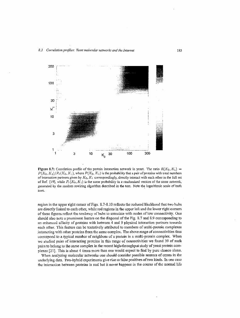
Figure 8.7: Correlation profile of the protein interaction network in yeast. The ratio R(K0, K1) = P ( K 0 , K1)/P,.(Ko, K I ) , where P(K0, KI) is the probability that apair ofproteins with total numbers of interaction partners given by KO, K1 correspondingly, directly interact with each other in the full set of Ref. [19], while P,(Ko, KI,) is the same probability in a randomized version of the same network, generated by the random rewiring algorithm described in the text. Note the logarithmic scale of both axes.

region in the upper right corner of Figs. 8.7-8.10 reflects the reduced likelihood that two hubs are directly linked to each other, while red regions in the upper left and the lower right corners of these figures reflect the tendency of hubs to associate with nodes of low connectivity. One should also note a prominent feature on the diagonal of the Fig. 8.7 and 8.9 corresponding to an enhanced affinity of proteins with between 4 and 9 physical interaction partners towards each other. This feature can be tentatively attributed to members of multi-protein complexes interacting with other proteins from the same complex. The above range of connectivities thus correspond to a typical number of neighbors of a protein in a multi-protein complex. When we studied pairs of interacting proteins in this range of connectivities we found 39 of such pairs to belong to the same complex in the recent high-throughput study of yeast protein complexes [21]. This is about 4 times more than one would expect to find by pure chance alone.

When analyzing molecular networks one should consider possible sources of errors in the underlying data. Two-hybrid experiments give rise to false positives of two kinds. In one case the interaction between proteins is real but it never happens in the course of the normal life

184

100 ;

30

%.It

10

3

1 1

8 Correlation Projles and Motifs in Complex Networks

3 Kin 10 30

Figure 8.8: Correlation profile of the transcription regulatory network in yeast.

2

I .5

I

1.5

3

The ratio R(Kout, ITz,) = P(K,,trK,,)/P,(IC,,t, K,,), where P(IC,,t, Kin) is the probability that aprotein node with the out-connectivity K,,t transcriptionally regulates the protein node with the in-connectivity IC,, in the network from the YF'D database [20], while P,(KoqLt, K,,) is the same probability in a randomized version of the same network, generated by the random rewiring algorithm described in the text. Note the logarithmic scale of both axes.

cycle of the cell due to spatial or temporal separation of participating proteins. In another case an indirect physical interaction is mediated by one or more unknown proteins localized in the yeast nucleus. Reversely, in a high throughput two-hybrid screens one should expect a siz- able number of false negatives. Primarily a binding may not be observed if the conformation of the bait or prey heterodimer blocks relevant interaction sites or if the corresponding heterodimer altogether fails to fold properly. In addition to this 391 proteins out of the potential 5671 baits in [19] were not tested as possible bait hybrids because they were found to activate transcription of the reporter gene in the absence of any prey proteins.

Fortunately, the qualitative features of the correlation profile are very robust with respect to an unbiased set of false positives and false negatives. Indeed, as previously undetected edges are added to the network (or falsely detected edges are removed from it) the average connec-

S.3 Correlation projles: Yeast molecular networks and the Internet 185

3 l U . ...-,.. ".

K~ 30 "IO 302)

Figure 8.9: Statistical significance of correlations present in the protein interaction network in yeast. The Z-score of correlations Z(Ko, KI) = (P(Ko,I--l) - P,(Ko, K I ) ) / ~ , ( K o , Kl) , where P(K0, K i ) is the probability that a pair of proteins with total numbers of interaction partners given by KO, 1-1 correspondingly, directly interact with each other in the full set of Ref. [ 191, while P, (KO, K1)

is the same probability in a randomized version of the same network, generated by the random rewiring algorithm described in the text, and cr,.(Ko, K1) is the standard deviation of P,(&, K1) measured in 1000 realizations of a randomized network. Note the logarithmic scale of both axes.

tivity of its nodes changes. As a result correlation features visible in its correlation profiles may shift their positions and intensity, but are likely to preserve their qualitative characteristics up to a very high level of false positives or false negatives.

The data for the protein interaction network used in this work come from a high-throughput experiment performed in one lab using a unique experimental technique [ 191. This fact makes it a perfect candidate for correlation profiling. Indeed, since almost all pairs of yeast proteins were tested as potential interacting partners, the statistical information contained in the resulting network contains no anthropomorphic bias. On the other hand, when the information about edges in a network is obtained from a database, combining results of many experimental groups using various techniques, one should wony about a hidden anthropomorphic factor: some proteins just constitute more attractive subjects of research and are, therefore, relatively

186

100

30

.?" xo

10

3

1

8 Cowelatiori Projles and Motgs i?i Conzplen Netw0r.h

10 30 Kin 3

8

6

4

2

0

-2

-4

-6

-8

Figure 8.10: Statistical significance of correlations present in the transcription regulatory network in yeast. The ratio Z(KOtLt, Kin) = (P(KolLt, Kin) - Pr(KOILt, Kin))/ar(KoIrt,ICin)), where P(Kout, Kin) is the probability that a protein node with the out-connectivity KoTLt transcriptionally regulates the protein node with the in-connectivity Kin in the network from the YPD database [20], while P, (KOtLt, .Kin) is the same probability in a randomized version of the same network, generated by the random rewiring algorithm described in the text, and cr(ICoTLt, Kin) is the standard deviation of P,.(K,,t, Kin) measured in 1000 realizations of a randomized network. Noste the logarithmic scale of both axes.

better studied than the others. The level of clustering in networks based on the database data may be overestimated due to several reasons: 1) With the exception of systemwide experiments such as high-throughput two-hybrid screens in yeast [22, 191, experimentalists are more likely to check for interactions between pairs of proteins within the same functional group. 2) A complete analysis of all possible painvise interactions within a small group of proteins would influence the level of clustering in the network. In this case this group would manifest itself by a relatively dense pattern of interactions with other members of the same group compared to interactions outside of the group.

A good example to illustrate the danger of indiscriminately using the database data is given by the network of physical interactions among yeast protein listed in 1231. This database contains contributions from several high throughput two-hybrid experiments [19, 221 as well as protein interactions determined by other methods such as co-immunoprecipitation technique,

8.3 Col7slatioitprofiles: Yeast molecular iiehvorks and the Internet 187

and mass spectroscopy of protein complexes. Statistical properties of this network were an- alyzed in a recent preprint [24], where it was shown that it has a remarkably high clustering coefficient. The clustering coefficient of a network is given by the number of triangles normalized by the total number of places in the network, where a triangle can be formed. When we constructed a correlation profile of this network we found that it contains a pronounced red linear region all along the diagonal of the 1io-K~ plane. Such a region corresponds to an increased affinity of proteins of a given connectivity to others with approximately the same value of connectivity. However, a closer analysis has revealed that this feature is an artifact of the way that interactions among complex-forming proteins were reported in this particular database. Apparently, an interaction was reported between any hvo proteins which were found to belong to the same multi-protein complex. Hence, all members of a given multi- protein complex consisting of N, proteins have connectivity close to N,. Needless to say this artificial feature would lead to a gross over counting of the clustering coefficient reported in Refs. [24]. In reality protein in a large multi-protein complex directly interact with no more than a few members of the same complex, which gives rise to a red spot on the diagonal of R( KO, K1) for intermediate values of KO and (see Fig. 8.7).

Correlation profiles similar €0 those presented in Figs. 8.7-8.10 can be constructed for any network. In what follows we measure them in the Internet connectivity network on the level of so-called Autonomous Systems (AS). An Autonomous System is a group of workstations, servers, and routers belonging to one organization such as e.g. a university, a company, or an Internet Service Provider. Connections between such Autonomous Systems are achieved by the virtue of the Border Gateway Protocol (BGP), which establishes which other AS a given AS directly communicates with and what kind of routing information is exchanged in the course of these communications. Daily data about connections between individual Au- tonomous Systems are available at the website of the National Laboratory for Applied Net- work Research (NLANR) [25]. In our analysis we used the information about the network of Autonomous Systems collected on January 2,2000. This data set consists of 12572 symmetric connections between 6474 AS. It is a scale-free network in which the power law connectivity distribution p ( k ) N k-7 withy = 2.2 f 0.1 spans over 3 orders of magnitude in k [5].

An ensemble of 1000 randomized networks with the same connectivities of individual nodes was generated by the random rewiring algorithm described in the previous section. The corresponding R- and Z- correlation profiles are shown in Figs 8.1 1-8.12. From these figures one infers that the Internet is characterized by the following set of correlations:

1. Strong suppression of edges between nodes of low connectivity 3 2 KO, K1 2 1.

2. Suppression of edges between nodes that both are of intermediate connectivity 100 > K O , K1 2 10,

3. Strong enhancement of the number of edges connecting nodes of low connectivity 3 1 KO 2 1 to those of intermediate connectivity 100 > K1 2 10.

On the other hand any pair among 5 hub nodes with KO, IC1 > 300 was found to be connected by an edge, both in the real network, and in a typical random sample. Hence I?(&, K l ) is

188 S Cowelatio?i Profiles and Motifs ill Coniplex Netwoih

3000

3 000

300

100 K,

3c

10

2

1 1 3 30 100 300 1000 3L-3

KO

Figure 8.11: Correlation profile of the Internet. The ratio R(Ko, Kl) = P(K0, KI)/P,(Ko, KI), where P(&, K1) is the probability that a pair of AS with connectivities KO and K1 to be nearest neighbors of each other in the Internet, while PT(I<o, Kl) is the same probability in a randomized version of the same network, generated by tlie random rewiring algorithm described in tlie text. Note the logarithmic scale of both axes.

close to 1 in the upper right comer of Fig. 8.1 1. The strong suppression of connections between pairs of nodes of low connectivity can in part be attributed to the constraint that all nodes on the Internet have to be connected to each other by at least one path. We have explicitly checked that there are indeed no isolated clusters in OF data for the Internet. However, when we used an ensemble of randoin networks in which the foilnation of isolated clusters was prevented at every rewiring step, we found little change in the observed correlation profile.

The pattern of correlations observed in the Internet is consistent with a picture of multi- level hierarchy among its nodes. Indeed, based on their connectivity Autonomous Systems can be loosely separated into several hierarchical levels [26], which starts from “user level” AS of very low connectivity connected to regional, national, and international Internet Services Providers with increasing ranges of connectivity. From the correlation profile described above one infers that user level AS tend to connect to intermediate level AS (regional ISP) and that the &ally large ISP are all linked to each other by peer-to-peer connections.

The Internet is a convenient example to illustrate the difference between randomized version of the network generated by local randomization algorithms [ 15,13,12] in which multiple

8.3 Correlation profiles: Yeast molecular networks and the Internet 189

300

1 OD K,

30

10

1 3 10 30 100 KO

20

1 0

-20

-30

-40 n 350 1000 3t-u

Figure 8.12: Statistical significance of correlations present in the Internet. The Z-score of correlations ~ ( K o , T i l ) = (P(Ko, K1) - P,(Ko,KI))/G(Ko, K I ) , where P(K0, K I ) is the probability that a pair of AS with connectivities KO and K1 are nearest neighbors of each other in the Internet, while P, (KO, K1) is the same probability in a randomized version of the same network, generated by the random rewiring algorithm described in the text, and o+(&, IC1) is the standard deviation of P,(I<o, IC l ) measured in 1000 realizations of a randomized network. Note the logarithmic scale of both axes.

edges are forbidden, and the truly uncorrelated randomized version of the network generated by the stub reconnection algorithm [16, 91, which inevitably has multiple edges. In complex networks characterized by a broad connectivity distribution the stub reconnection algorithm usually results in multiple edges between hub nodes. In a network with E edges in total, the probability that the stub reconnecting algorithm would create a multiple edge between a pair of nodes with connectivities If0 and Kl becomes substantial if K o K 1 / ( 2 E ) > 1. Since in scale- free networks characterized by a power law distribution of node connectivities p ( k ) - k-Y the connectivity of a few highest connected nodes in the system scales as N'/(Y-l), the expected number of edges between a pair of such hub nodes scales as N2/(Y-')/E N N2/(Y-')-' becomes significant for the large number of nodes N provided that y < 3. For example, in a randomized version of the Internet generated by this algorithm the expected number of edges connecting the two highest connected hubs of respectively KO = 1458 and IC1 = 750 is a swooping KoK1/(2E) = 1458 .750/ (2 . 12572) = 43.5! This means that in a randomized version of the Internet with no multiple connections between nodes the connectivity between

190 8 Correlatioii Projles and Mot$s in Complex Nehvorlcs

these hub nodes would be suppressed by a factor of 43 relative to a random network allowing for multiple edges. Thus the ban on multiple connections between a given pair of nodes gives rise to an effective ''repulsion'' between hubs in such a randomized network. To quantify the level of this repulsion we measured the average connectivity (Kl)li, of neighbors of sites with connectivity KO as a h c t i o n of KO in the real Internet network (squares in Fig. 8.13 j as well as in an ensemble of random networks with no multiple connections between nodes generated by the local rewiring algorithm (circles in Fig. 8.13.) From this figure it is clear that most of the ( K ~ ) K ~ K dependence reported in Ref. [27] is reproduced in our random ensemble and hence can be attributed to the above mentioned effective repulsion between hubs due to the constraint of having no more than one edge directly connecting them to each other. It is worthwhile to note that in the random network generated by the stub reconnection algorithm ( K ~ ) K ~ = (I<1.2)/(K1) 21 165 would be independent of KO.

Let p ( K ) be the probability distribution of connectivities in the complex network and let us consider its random counterpart generated by stub reconnection algorithm [ 16,9]. Since in this algorithm each of the two nodes is independently selected to form a connection through one of its edge stubs, the probability to pick a node with connectivity K is given by K p ( K ) / ( K ) , and the conditional probability distribution P$"b(l(l [.KO) is independent of KO and equal to

P,""""K1lKrJ) = Klp(Kl) / (K) . (8.61

On the other hand, in an ensemble of random scale-free networks with no multiple edges the conditional probability distribution P(I(1 IKo) crosses over between K1/p(l(l) functional form for K1 << Kf = 2E/Ko to p(K1) for K1 >> I<-:. We have confirmed numerically that P(K1 I KO) in our randomized ensemble has a very similar shape to that observed in the real Internet [28] thus once more verifjmg that most of correlation effects visible in the internet network can be attributed to the effective repulsion between hubs due to the constraint of no multiple connections. The remaining correlations are quantified in the correlation profile in Figs. (8.11,8.12).

8.4 Network motifs: Transcriptional regulation in Exoli A fundamental question in understanding a complex network is whether it can be decomposed into building blocks. Ideally, such building blocks would be well separated from each other, and thus the entire network dynamics could be approximated by a combination of dynamics of these basic elements.

A natural place to examine this question further is the best characterized biological regulation network, that of transcription regulation in the bacterium E. coli [29, 301. In this network, the nodes are operons (groups of genes transcribed form a single mlZNA). Some of the operons encode for regulatory proteins, which regulate the transcription rates of certain other operons. Thus, each edge is directed from an operon encoding a regulatory protein to an operon regulated by that protein.

The transcription network of E. coli has a broad scale-free-like distribution of outgoing edges, and a compact distribution of incoming edges. The resulting directed graph shown in Fig. 8.1 appears quite complex, as seen by plotting it with a standard graph display algorithm [2] (the dataset is available at www.weizmann.ac.il/mcb/UriAlon). We note that transcription

8.4 Network motifs: Panscriptioiial regulation in E.coli 191

1 oo 1 oo 10' 1 o2 1 o3 1 o4

KO

Figure 8.13: The average connectivity of a neighbor (K1) vs the connectivity of a node KO in the Internet (squares) and its randomized version with no multiple edges (circles). The error bars in multiple realizations of the randomized network are smaller than the size of the symbol.

graphs have an additional color for each edge: each regulatory protein can be a positive or a negative reguIator, termed activator or repressor respectively (in rare cases a dual regulation is found). To detect recurring patterns in this graph that are likely to have a functional role, a new approach based on network motifs was recently presented [14]. The approach is simple to define: one enumerates the appearance of all types of subgraphs in the graph. The number of appearances of each subgraph is then compared to an ensemble of randomized networks, generated as discussed in section 2, such that each of the randomized networks preserves the incoming and outgoing edge degrees for each node. Network motifs are subgraphs that satisfy a statistical-significance criterion: the probability that they appear in a randomized graph more often than in the real graph is smaller than a threshold P-value (eg P < 0.01). The profile of the network given by the set of such statistically significant network motifs nicely compliments the correlation profile described in the previous section.

a. Type I patterns: Patterns with no free structural parameters. This involves full enumera- tion of small subgraphs: all 13 types of 3-node connected, directed subgraphs, and 199 types

Here we review the representation of 3 particular kinds of patterns:

192 8 Correlation Projles and Motifs in Conzpla Networks

of 4-node subgraphs were enumerated in Ref [14]. The complexity rises exponentially for larger subgraphs, and efficient Monte-Carlo sampling methods still need to be devised for completely enumerating all types of n-node directed subgraphs. The algorithms for type-I- pattern detection can either take into account or ignore the edge colors. As shown below, the dynamical behavior of each subgraph may critically depend on the edge coloring. b. Type II patterns: Patterns with a free structural parameter. Visual examination of the transcription network showed a recurring pattern: a set of nodes with only one incoming edge, all from the same master node. In Ref. [ 141 such patterns were termed Single Input Modules (SIM) since no node other than the master node regulates any of the nodes in this pattern. This pattern has a free structural parameter, the number of nodes in the SIM. An algorithm that searches for this pattern (and in general for identical rows in the connectivity matrix of the graph) was employed for comparison with randomized graphs. Taking edge color into account, the definition of SIMs is further restricted to the case where all edges have the same color (that is all negative or all positive regulation). c. Type IIT patterns: Classes of patterns defined by an extensive characteristic such as edge density. In the present case, a clustering approach was defined for cdetecting regions in the graph that are more dense then in randomized graphs. This defined Dense Overlapping Reg- ulons (DOR). A regulon is a biological term for a set of operons all regulated by the same regulatory protein, not necessarily exclusively [3 11. Naturally, other pattern classes can be defined in this way.

First let us summarize the overall findings of this detailed analysis of network motifs: In regards to type I patterns it was found that out of 13 possible 3-node subgraphs only one is statistically significant. This motif was termed the Feed-Forward Loop (FFL) (Fig. 8.14), and the real network had 40 of these as compared to the 7 =k 5 found in an ensemble of randomized networks. Of the 4-node subgraphs, only one was significant, a pattern with 4 edges representing overlapping regulation X i W, 2 and Y + W, 2. This 4-node motif hints that dense overlapping regions are extant in the network. This was indeed found to be the case, but the dense region broke down into 6 weakly overlapping dense clusters, the type 111 patterns termed DORs (Fig. 8.14~). Finally, among the the type I1 patterns, large SIMs were found to be highly significant (Fig. 8.14b).

To further validate the motifs it was tested [14] whether they are sensitive to data er- rorshncomplete data. As in the case of correlation profiles discussed in the previous section, it was found that the statistical significance of the network motif is highly robust with respect to data errors. For example, when over 30% of the connections are removed at random, or added at random, all 3 motifs remain significant and no new motifs appear in the network. This robustness may fail, of course, if the dataset contains systematic errors with a bias for certain kinds of patterns. For example, well-known regulatory proteins are investigated by inany labs, which may result in a tendency for an increased number of known connections for these nodes (an effect similar to searching for the coin under the streetlamp). This inay exaggerate the number of SIMs detected. The, existence of SIMs was also hinted at by the correlation profile of yeast regulatory network discussed in the previous section. Indeed, the abundance of SIMs must be at least partially responsible for the observed preference of highly

5.4 Network motifs: Transcriptional regulation in E.coli 193

a. Feedfonvard loop (FFL) c. Dense overlapping regulons (DOR)

f Z

b. Single input module #Edges/#nodes >> than random clusters

+T* ;,y

Z1 22 Zn Figure 8.14: The three network motifs in the E. coli transcription network.. In this figure, the edge colors (regulation signs) are not shown. a) Feed-forward Loop (FFL). b) Single Input Module (SIM) where X regulates n output nodes. The output nodes have no other incoming edges. All regulations are of the same sign. c) Dense Overlapping Regulon @OR). A set of input nodes X1 ... Xm regulates a set of output nodes ZI ... Zn, with a resulting cluster of edges that is much denser than those found in randomized networks. In [14], a clustering algorithm that clusters nodes according to the number of overlapping inputs was presented, and used to compare the DOR structures to the randomized ensemble.

connected proteins (hubs) to connect to neighbors with lower than average connectivity in this network. The fact that the preference of proteins with low and high connectivity to connect to each other was also observed in both the protein interaction and regulatory networks in yeast indicate that, perhaps, SIMs are a significant feature in all types of bio-molecular networks.

Over SO% of the nodes in the E.coli transcription network belong to one of the three motifs defined above, FFL, SIM or DOR. The remaining nodes usually belong to tiny disjoint components of 1-3 nodes. Thus the decomposition of the network into recurrent motifs allow us an alternative way to present the data, in terms of its structure, and of the relative position of the various motifs (Fig. 8.15). A small set of nodes with an outgoing edge degree much larger than average (global regulators) complicates the graph image. An important step in visualizing the network is to allow the nodes with high output degrees to appear multiple times in the image, acting as inputs to the various DOR structures in which they participate. This preserves all of the information but removes many complicating edges. It is seen that the transcription network of E. coli is mostly a two-layer feed-forward network. The FFLs and SIMs are often at the outputs of the DORs. These two motifs are therefore integrated into the DOR structures.

Dynamical behavior of network motifs: Two of the motifs, FFL and SIM, have been shown to carry out distinct information processing functions, using numerical simulations [14]. The SIM motif allows the operons to be turned on in a particular temporal order and turned off in the reverse order, akin to the “First-In Last-Out’’ (FILO) pipeline. The temporal

194 8 Correlation Profiles and Motys in Conplen: Networks

w

m

Figure 8.15: The complete known E. coli transcription network displayed using network motifs. This version has several corrected edges and several new nodes as compared to the images in [14]. The complete dataset is available at w\.vw.weizmann.ac.il/mcb/UriAlon

5.4 Netwodc motifs: Traiwcriptioizal regulation in E.coli

a. Cohesent feedfoiward loops

195

X

Y

Z

--X

j:

Y

1 -iZ

b. Incoherent feedforward loops

Figure 8.16: Coherent (a) and Incoherent (b) feed-forward loops. Arrows represent positive regulation, and -1 symbols represent negative regulation (repression).

order is encoded in the relative strengths of the edges to each node (mechanistically, in the strength and position of regulatory protein and RNA polymerase binding sites in the regulatory DNA region that precedes each operon). To understand the dynamics of the FFL motif, the edge coloring becomes important. When taking into account the two edge colors, there are 8 possible colorings of the FFLs three edges. However, it is sufficient to consider two types of FFLs. The FFL is composed of a direct path from node X to node Z, and an indirect path through node Y. A coherent FFL has the same sign on the direct path as the net sign of the indirect path (Fig.8.16a), while an incoherent FFL has opposing signs in the direct and indirect paths (Fig 8.16b). The coherent FFL is the dominant form in E. coli (P < 0.001), while the incoherent FFL is only marginally significant ( P N 0.03). The two types of FFL motifs can show very different dynamical behavior. For simplicity we consider here the case where the two inputs act as an AND gate to control the output Z, a typical case in transcription systems. The coherent feed-forward loop acts to reject rapid input pulses of X that go from OFF to ON, responding only to persistent inputs. However, there is a strong response even to short reverse pulses from ON to OFF. Thus the coherent FFL can act as a sign-sensitive filter. The condition for this is that the level of Y in the OFF state of X is below the activation threshold for Z. The typical width of pulses first passed by this filter is given by the time it takes Y to cross Z's activation threshold.

196 S Correlation Projles and Motijis in Complex Networks

The incoherent FFL can act as a sign-sensitive differentiator (pulse generator). In a step where X goes from OFF to ON, Z is rapidly activated. Then, Y levels build up to cross the repression threshold for Z. Thus after a delay, Z becomes inactivated, given that the negative effect of Y is strong enough. On the other hand, no response is seen in a step from ON to OFF,

These two functions, sign-sensitive filtering and temporal transcription programs, may be basic tasks in the information processing performed by E. coli. Indeed, it has recently been found experimentally .that temporal programs exist in systems such as flagella bio-synthesis [32] and SOS DNA repair (Ronen, Rosenberg, Shraiman, Alon, submitted 2002), where the temporal order within groups of operons controlled by. the same regulator corresponded to the functional order of these genes. The STM mechanism is likely to be at play.

These findings can point the way to experiments designed to understand the hnctions of each motif. Once these functions are understood, one may check whether the dynamics of the entire network can be well approximated as a combination of the dynamics of its separate motifs.

.. where Z remains suppressed.

8.5 Discussion: What it may all mean? The large scale organization of molecular networks deduced from correlation profiles of protein interaction and transcription regulatory networks in yeast, and the set of statistically significant network motifs in the regulatory network of E.coli is consistent with compartmental- ization and modularity characteristic of many cellular processes [33]. Indeed, the suppression of connections between highly connected proteins and the abundance of DOR network motifs both suggest the picture of semi-independent modules centered around or regulated by individual hubs. On the other hand, the very fact that these molecular networks do not separate into many isolated components but are dominated by one “giant component” suggests that this tendency towards modularity is not taken to its logical end. It can in fact be described as “soft modularity”, in which interactions between individual modules are suppressed but not completely eliminated. Thus on sufficiently large scale molecular networks exhibit system properties making their behavior different from that of a set of mutually independent modules. Two recent observations independently hint at global interrelations in the overall connectivity pattern of molecular networks:

1. Elena and Lenski [34] studied the cooperativity of regulation in E.coJi by comparing changes of the cell cycle length in single-gene null mutants with those in double null mutants. They concluded that about 30% of gene pairs exhibited more than additive effects on cell cycle length, and thus at least 30% of protein pairs are functionally in- terconnected. Such level of cooperativity would be impossible in a regulatory network consisting of a large number of independent modules.

.

2. C.K. Stover et al. [35] found that the number of transcription factors (Nt,) in procaiyotic organisms grows as a square of the number of genes N : Nt, oc N 2 . Hence, each additional gene (or gene module/regulon) appears to be regulated with respect to all genes that are already present. This indicates an overall regulation pattern that on sufficiently large scale is neither modular, nor hierarchic.

8.5 Disciission: What it may all mean? 197

On the other hand, in this work we demonstrated that already on the level of the correlation profile (the two point correlation function) these networks exhibit a certain degree of modularity. A further implication of those modular features manifested by the deficit of connections between highly connected proteins (Figs. 8.7, 8.8) is in the suppression of propagation of deleterious perturbations over the network. It is reasonable to assunie that certain perturbations such as e.g. a significant change in the concentration of a given protein (including it vanishing altogether in a null-mutant cell) with a ceratin probability can affect its first, second, and sometimes even more distant neighbors in the corresponding network. While the number of immediate neighbors of a node is by definition equal to its own connectivity KO, the average number of its second neighbors is bound from above by KO ((Kl - 1)}1~, and thus depends on the correlation profile of the network. In addition it is sensitive to higher order correlation patterns of the network. For example, in the presence of a significant level of clustering the number of second neighbors can fall well below the above mentioned upper bound. Since highly connected nodes serve as powerhl amplifiers for the propagation of deleterious perturbations it is especially important to suppress this propagation beyond their immediate neighbors. It was argued that scale-free networks in general are very vulnerable to attacks aimed at hubs [36,37]. The deficit of edges directly connecting hubs to each other reduces the branching ratio around these nodes and thus provides a certain degree of protection against such attacks.

To summarize the above discussion, it is feasible that molecular networks operating in living cells have organized themselves in an interaction pattern that is both robust and specific. Topologically the specificity of different functional modules is enhanced by limiting interactions between hubs and suppressing the average connectivity of their neighbors. Such correlations are also evident on a more detailed level of local structural motifs such as SIMs and DORs. Each of those network motifs has certain computational properties providing the cell with appropriate responses to environmental and internal changes. On a larger scale there is evidence for interconnections between these modules, although the principles of such global organization of living cells remain unclear from the present day data and analysis tools.

Correlation profiles and statistically significant network motifs allow one to distinguish between different complex networks, even if their connectivity distributions appear identical. Thus, for example, the Internet at the level of Autonomous Systems and physical interactions among yeast proteins are both characterized by power-law connectivity distributions with rather similar exponents. However, correlation profiles of these two networks (Figs. 8.7, 8.1 l), are qualitatively different from each other. First, in the Internet unlike in molecular networks, connections between the highly connected nodes were not suppressed. In fact any pair of hubs on the Internet was connected to each other by a direct link. Secondly, the protein interaction network in yeast is characterized by an enhancement of connections between nodes with intermediate connectivities , as opposed to the Internet, where such connections were found to be strongly suppressed. Also, unlike protein interaction networks the Internet has a deficit of edges connecting nodes of very low connectivity to each other. This all indicates that the information processing mechanisms relevant to protein interaction networks are qualitatively different from those relevant to the Internet.

19s S Correlation ProJiles and Motifs in Conzplex Networks

The main goal of the present work was to introduce a number of statistical tools necessary for analyzing topological patterns and correlations in networks. These tools allowed us to identify the set of different topological patterns and characteristic building blocks (motifs) present in a broad range of complex networks, which may help to better understand possible mechanisms for their function and evolution. The advantage of our approach lies also in it iterative nature in which the understanding of more and more complex topological properties of the network gradually builds up on the analysis of its lower level featurgs, Work s6pporTed by the U.3: Department oFEnergy under Contract No. DE-AC02-98CH10886.

- -- - - - -

References [ 13 For an overview see e.g. other chapters of this book. [2] V. Batagelj, A. Mrvar, Pajek - Prograin for Large Network Analysis, Connections 21 2,

[3] P. Erdos, A. RCnyi, On the evolution of randoin graphs, Publ. Math. Inst. Hung. Acad.

[4] A.-L. Barabasi, R. Albert, Emergence of scaling in randoin networlis, Science, 286,509-

[5] M. Faloutsos, P. Faloutsos, and C. Faloutsos, Comput. Commun. Rev. 29,251 (1999). [6] A. Broder, et al., Graph Structure in the Web, Computer Networks, 33,309-320 (2000). [7] H. Jeong, B. Tombor, R. Albert, Z. N. Oltvai, A.-L. Barabasi, The large scale organiza-

tion of methabolic networks, Nature, 407, 651-654 (2000). [SI H. Jeong, S. Mason, A.-L. Barabasi, Z.N. Oltvai, Centrality and lethality of protein

networks, Nature 411,4142 (2001). [9] M. E. J. Newman, S. H. Strogatz, and D. J. Watts Randoin graphs with arbitrary degee

distributions and their applications, Phys. Rev. E, 64,0261 18, 1-17 (2001): See also the chapter by M. E. J. Newman in this book.

[lo] D. Watts and S. Strogatz, Collective Dynamics of Small World Nehvorks, Nature 293, 400 (1998).

[l I] S. Wasserman and K. Faust, Social NetworkAnalysis, Cambridge University Press, 1994. [12] S. Maslov and K. Sneppen, Pattern Detection in Conzplex Networks: Correlation Profile

of the Internet, cond-matl0205379, submitted to Physical Review Letters (2002). [13] S. Maslov and K. Sneppen, SpeciJicity and Stability in Topology of Protein Networks,

Science 296 910-913, (2002). [ 141 S.S. Shen-Orr, R. Milo, S. Mangan, and U. Alon, Network motiji in the franscriptional

regulation of Escherichia coli, Nature Genetics, 31(1):64-68 (2002). [ 151 Early studies of these algorithms were reported in: D. Gale, A theorern offlows in net-

works, Pacific J. Math., 7, 1073-1082 (1957); H.J. Ryser, Matrices ofzeros and ones in combinatorial inatheinatics, in “Recent Advances in Matrix Theoiy ”, pp. 103-124, Univ. of Wisconsin Press, Madison, (1964). For more recent references see e.g.: R. Kannan, P. Tetali, S. Venipala, Simple Markov-chain algoritlzins for generating bipartite graphs and tournaments, Random Structures and Algorithms 14,293-308, (1999).

[ 161 E.A. Bender and E.R. Canfield, The asymptotic number of labeled graphs with given degree sequences, Journal of Combinatorial Theory A, 24,296-307 (1978).

47-57 (1998)

Sci. 5, 17UGO (1960).

512 (1999).

References 199

[17] The set of MATLAB programs can be downloaded at http ://cmth .phy. bnl . gov/ maslov/matlab. htm

[18] M. Molloy and B. Reed, Random Struct. Algorithms 6, 161 (1995); M. Molloy and B. Reed, Combinatorics, Probab. Comput. 7,295 (1998).

[ 191 T. Ito, et al., A comprehensive two-hybrid analysis to explore the yeast protein interac- tome, Proc. Natl. Acad. Sci. USA 98,45694574 (2001).

[20] M. C. Costanzo, et al., YPD, PombePD, and WorinPD: rnodel organism volumes of the BioKnowledge library, an integrated resource for protein information, Nucleic Acids Research 29 75-79 (2001).

[2 11 A.-C. Gavin, et al., Functional organization of the yeastproteoine by systematic analysis oj-protein con2plexes, Nature 415, 141 (2002).

[22] P. Uetz, et al., A coinprehensive anallvsis of protein-protein interactions in Saccha- rornyces cerevisiae, Nature 403, 623-627 (2000).

[23] The supplementary materials to B. Schwikowski, P. Uetz, and S. Fields, A network of protein protein interactions in yeast, Nature Biotechnology 18, 1257 - 1261 (2000).

[24] A. Vazquez, A. Flainmini, A. Maritan, and A. Vespignani, Modeling of protein interaction networ/is, cond-mat/0108043 (2001).

[25] Website maintained by the National Laboratory for Applied Network Research (NLANR) Measurement and Network Analysis Group at http://moat.nlanr.net/

[26] The idea of deducing the hierachial level of an AS from its connectivity was proposed in: R. Govindan and A. Reddy, Analysis of internet inter-domain topology and route stabilifv, In Proceedings of the IEEE Infocom, pages 851-858, Kobe, Japan, April 1997, avaliable for download at http://citeseer.nj .nec.com/govindan97analysis.html, and later elaborated e.g. in L. Gao, On iizferring autoizomoiis system relationships in the Internet, in Proc. IEEE Global Internet Symposiuni, November 2000, avalaible for download at http://citeseer.nj .nec.com/gaoOOinferring.html.

[27] R. Pastor-Satorras, A. Vazquez, A. Vespignani, Dynainical and Correlation Properties of the Internet, Phys. Rev. Lett. 87,258701 1-4 (2001).

[28] K.-I. Goh, B. Kahng, and D. Kim, Phys. Rev. Lett. 88, 108701 (2002). [29] D. T h i e w , A.M. Huerta, E. PCrez-Rueda, & J. Collado-Vides, Froin spec@ gene reg-

ulation to global regulatory networh-s: a characterization of Escherichia coli transcriptional network, BioEssays20,433-440 (1998).

[30] A.M. Huerta, ’H. Salgado, D. Thieffry & J. Collado-Vides, RegulonDB: A database on

[3 11 F. C. Neidhardt and M. A. Savageau, Regulation bqond the operon. In “Escherichia coli and Salnzoizella typhiniuriunz: Cellular and Molecular Biology, ” Vol. 1 (F. C. Neidhardt, Ed.), pp. 1310-1324, Am. SOC. Microbiol., Washington DC (1996).

[32] S. Kalir, K. McClure, C. Pabaraju, C. Southward, M. Ronen, S. Leibler, M.G. Surette and U. Alon, Ordering genes in a flagella pathway by analysis expression kineticsfiom living bacteria. Science 292,2080-2083 (2001).

[33] L.H. Hartwell, J.J. Hopfield, S. Leibler, and A.W. Murray, Froin molecular to nzodular cell biology, Nature 402 (6761 Suppl), C47-52 (1999).

. transcriptional regulation iiz Escherichia coli Nucleic Acid Res. 26 (1998), 55-59.

200 8 Correlation ProBles and Motgs in Complex Networks

[34] S.F. Elena & R.E. Lenski, Test of synergetic interactions among deleterious mutations in

[35] C.K.Stover, Conplete genome sequence of Pseudomonas aeriegiosa PAOI, an oppor-

[3G] R. Albert, H. Jeong, A.-L. Barabasi, Error and attack toleraizce of complex networks,

[37] B. Vogelstein, D. Lane, and A.J. Levine, Sur$ng the p53 network, Nature 408, 307-310

bacteria Nature 390,395-398 (1999).

tunistic pathogen Nature 406, 959-398 (2000).

Nature 406,378-382 (2000).

(2000).

8 correlation profiles and motifs in complex networks

Documents