8. z-transforms1 agenda r1. difference equations r2. z-transforms r3. discrete fourier transform r4....
TRANSCRIPT

8. Z-transforms 1
Agenda
1. Difference equations2. Z-transforms3. Discrete Fourier transform4. Power spectral density
8. Z-transforms 2
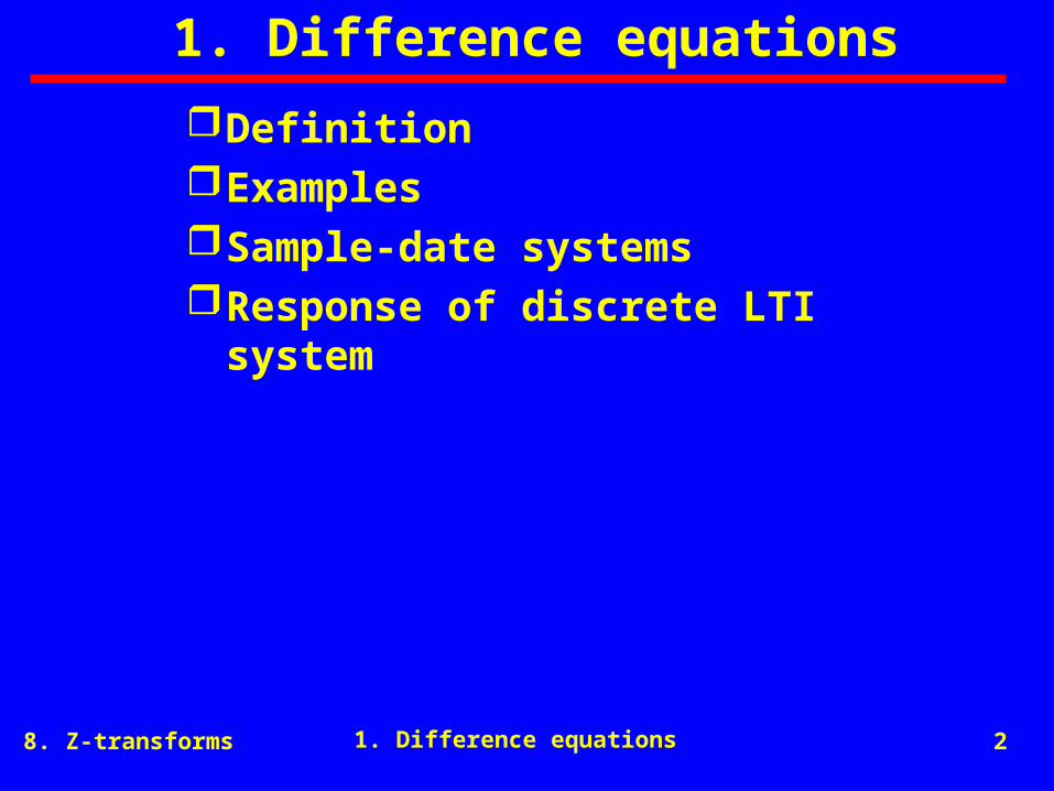
1. Difference equations
DefinitionExamplesSample-date systemsResponse of discrete LTI system
1. Difference equations
8. Z-transforms 3
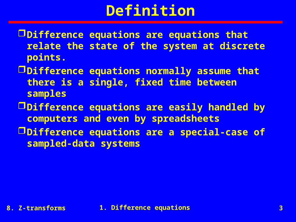
Definition
Difference equations are equations that relate the state of the system at discrete points.
Difference equations normally assume that there is a single, fixed time between samples
Difference equations are easily handled by computers and even by spreadsheets
Difference equations are a special-case of sampled-data systems
1. Difference equations

8. Z-transforms 4
Examples (1 of 4)
unitdelay
2
x[n] y[n]
y[n-1]
y[n] = 2 y[n-1] + x[n]y[n] - 2 y[n-1] = x[n]
A first-order, linear, time-invariant (LTI) difference equation
Example 1
1. Difference equations

8. Z-transforms 5
Examples (2 of 4)
unitdelay2
x[n] y[n]
q[n-1]
y[n] = q[n] + 4 q[n-1]q[n] = 2 q[n-1] + x[n]
4
q[n]
4 q[n-1] + q[n] = y[n] -2 q[n-1] + q[n] = x[n]
q[n-1] = 1/6(-x[n] + y[n]) q[n] = 1/3(2 x[n] + y[n])q[n-1] = 1/3(2 x[n-1] + y[n-1])
y[n] - 2 y[n-1] = x[n] + 4 x[n-1]
Example 2
1. Difference equations

8. Z-transforms 6
Examples (3 of 4)
unitdelay
2
x[n] y[n]
4
unitdelay
y[n] = 4 y[n-1] + 2 y[n-2] + x[n]
Example 3
y[n-1]y[n-2]
1. Difference equations

8. Z-transforms 7
Examples (4 of 4)
unitdelay
x[n] y[n]
1/3
unitdelay
y[n] = 1/3 (x[n] + x[n-1] + x[n-2])
1/3
1/3Example 4
x[n-1] x[n-2]
1. Difference equations

8. Z-transforms 8
Sample-data systems
A system that receives information intermittently
Sampling may be periodic, aperiodic, or random
State information is not available between samples
sampler
computerhold
circuitplant
x(t) e(t)
-+
y(t)
1. Difference equations

8. Z-transforms 9
Response of discrete LTI systemImpulse response• h[n] = T{[n]}
Arbitrary input
• x[n] = x[k] [n-k]Response to arbitrary input
• y[n] = T {x[n]} = T { x[k] [n-k] }
• = x[k] h[n-k]
• = convolution sum
k=-
k=-
k=-
1. Difference equations

8. Z-transforms 10
2. Z-transform
IntroductionZ transformationDefinitionTransformsExamples
2. Z-transforms

8. Z-transforms 11
IntroductionThe z-transform is the discrete-time
counterpart of the Laplace transformThe Laplace transform converts integro-
differential equations into algebraic equations.
The z-transform converts difference equations into algebraic equations
Properties of z-transforms parallel those of Laplace transforms, but there are important distinctions
2. Z-transforms

8. Z-transforms 12
Z transformation
lineardifference equation
timedomainsolution
z transformedequation
z transformsolution
time domain
summing
algebra
z transforminverse z transform
z domain orcomplex frequency domain
2. Z-transforms
8. Z-transforms 13
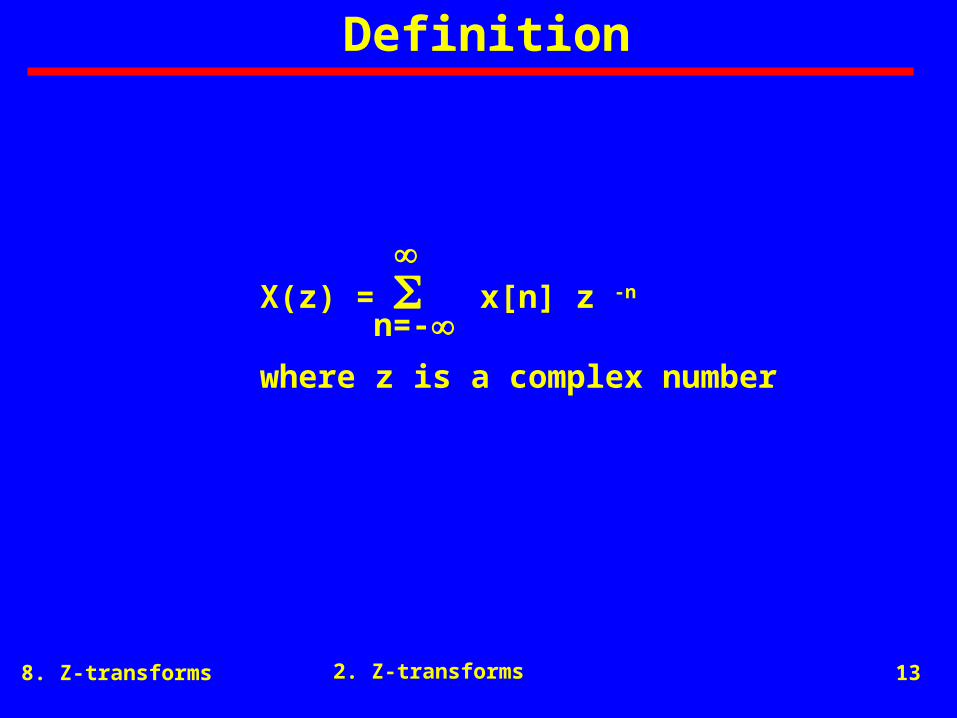
Definition
X(z) = x[n] z -n
where z is a complex number
n=-
2. Z-transforms
8. Z-transforms 14
Transforms (1 of 4)
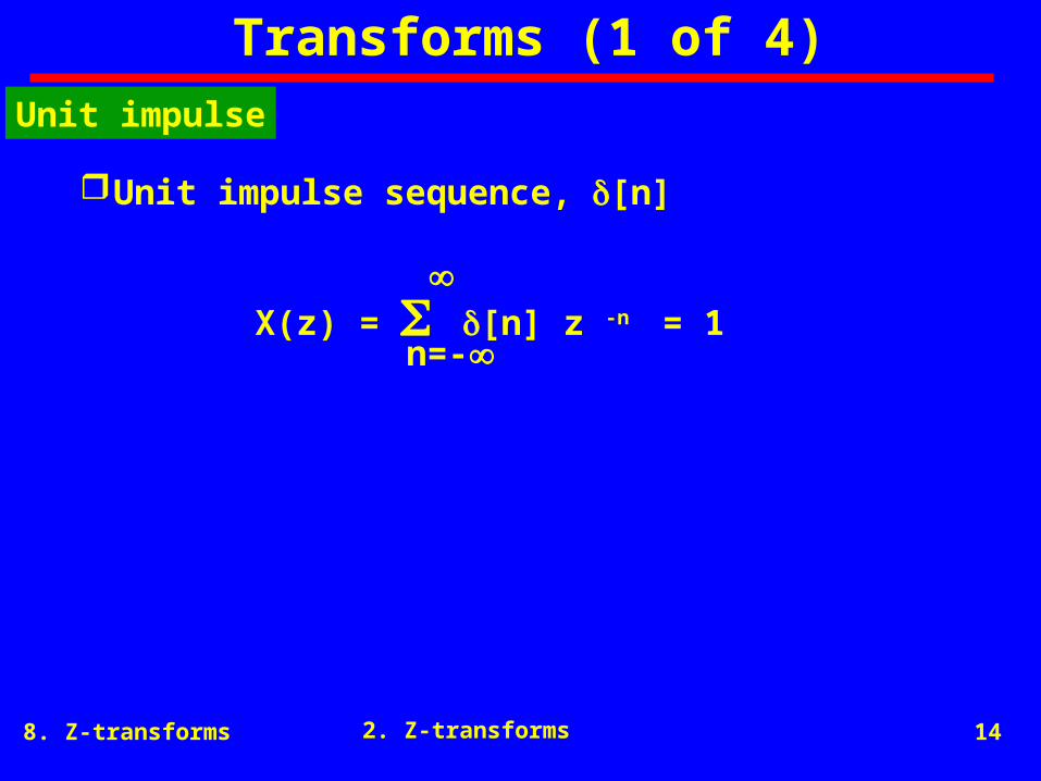
Unit impulse sequence, [n]
X(z) = [n] z -n = 1n=-
Unit impulse
2. Z-transforms

8. Z-transforms 15
Transforms (2 of 4)
Unit step sequence, u[n]
X(z) = u[n] z -n
= z -n
= 1/(1 - z-1)
= z/(z + 1)
n=-
0
Unit step
2. Z-transforms
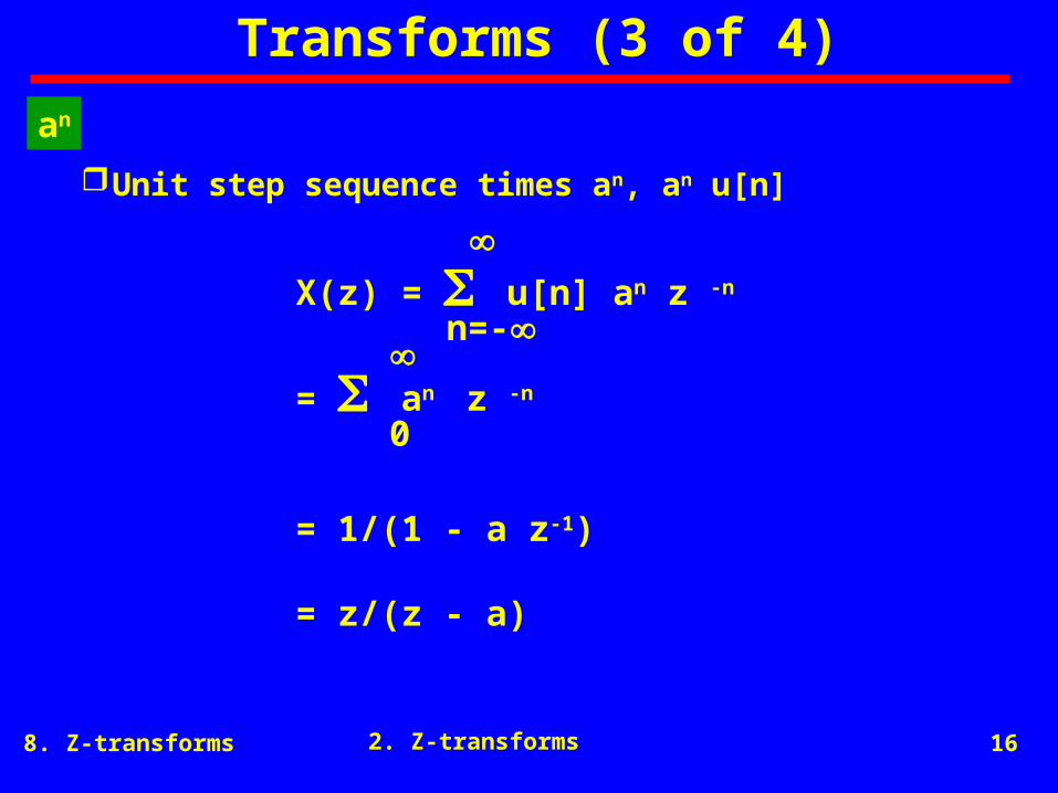
8. Z-transforms 16
Transforms (3 of 4)
Unit step sequence times an, an u[n]
X(z) = u[n] an z -n
= an z -n
= 1/(1 - a z-1)
= z/(z - a)
n=-
0
an
2. Z-transforms

8. Z-transforms 17
Transforms (4 of 4)
x1[n] x2[n]
x[n - m]
zon x[n]
z[-n]
x[n]
X1(z) ± X2(z)
z-m X(z)
X(z/zo)
X(1/z)
z/(z-1) X(z)
Linearity
Time shift
Multiplication by zon
Time reversal
Accumulation k=-
n
Properties
8. Z-transforms 18
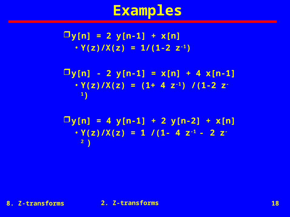
Examples
y[n] = 2 y[n-1] + x[n]• Y(z)/X(z) = 1/(1-2 z-1)
y[n] - 2 y[n-1] = x[n] + 4 x[n-1]• Y(z)/X(z) = (1+ 4 z-1) /(1-2 z-1)
y[n] = 4 y[n-1] + 2 y[n-2] + x[n]• Y(z)/X(z) = 1 /(1- 4 z-1 - 2 z-2 )
2. Z-transforms

8. Z-transforms 19
3. Discrete Fourier transform
DFTAliasingSampling theoremFrequency, resolution, and lengthLinear convolutionCircular convolutionBlock filteringFilteringWindowing
3. Discrete Fourier transform

8. Z-transforms 20
Inverse DFT
DFT
DFT (1 of 4)
X[k] = x [n] e -j(2/N)kn = x [n] WNkn
n=0
N-1
x[n] = 1/N X[k] e j(2/N)nk = 1/N X[k] WN-kn
k=0
N-1
n=0
N-1
k=0
N-1
WN = e -j(2/N)
Where
3. Discrete Fourier transform

8. Z-transforms 21
Matrix format
DFT (2 of 4)
X = DN x
1 1 1 1
1 WN1 WN
2 … WN(N-1)
1 WN2 WN
4 … WN2(N-1)
.
.
.
1 WN(N-1)(N-1) WN
(N-1)(N-1) … WN(N-1)(N-1)
X[0]
X[1]
X[2]
.
.
.
X[N-1]
=
x[0]
x[1]
x[2]
.
.
.
x[N-1]
3. Discrete Fourier transform
8. Z-transforms 22
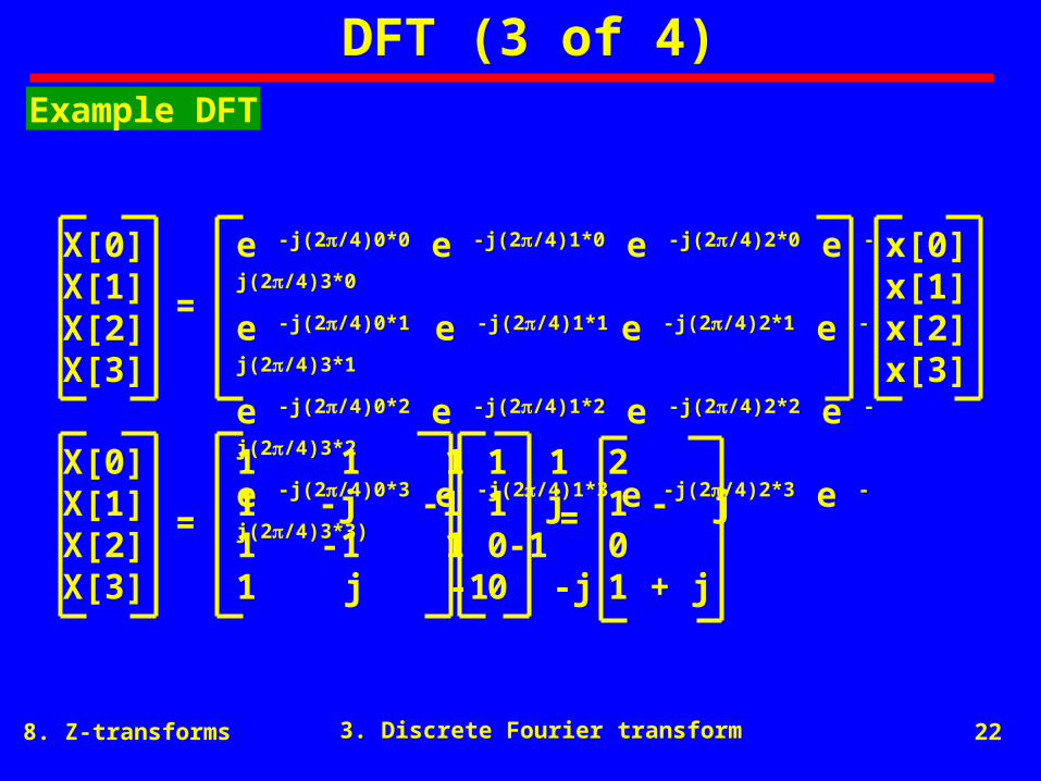
DFT (3 of 4)
e -j(2/4)0*0 e -j(2/4)1*0 e -j(2/4)2*0 e -j(2/4)3*0
e -j(2/4)0*1 e -j(2/4)1*1 e -j(2/4)2*1 e -j(2/4)3*1
e -j(2/4)0*2 e -j(2/4)1*2 e -j(2/4)2*2 e -j(2/4)3*2
e -j(2/4)0*3 e -j(2/4)1*3 e -j(2/4)2*3 e -j(2/4)3*3)
X[0]X[1]X[2]X[3]
=
x[0]x[1]x[2]x[3]
1 1 1 11 -j -1 j1 -1 1 -11 j -1 -j
X[0]X[1]X[2]X[3]
=
1100
=
21 - j01 + j
Example DFT
3. Discrete Fourier transform

8. Z-transforms 23
DFT (4 of 4)
e +j(2/4)0*0 e +j(2/4)1*0 e +j(2/4)2*0 e +j(2/4)3*0
e +j(2/4)0*1 e +j(2/4)1*1 e +j(2/4)2*1 e +j(2/4)3*1
e +j(2/4)0*2 e +j(2/4)1*2 e +j(2/4)2*2 e +j(2/4)3*2
e +j(2/4)0*3 e +j(2/4)1*3 e +j(2/4)2*3 e +j(2/4)3*3)
x[0]x[1]x[2]x[3]
=1/4
X[0]X[1]X[2]X[3]
1 1 1 11 +j -1 -j1 -1 1 -11 -j -1 j
x[0]x[1]x[2]x[3]
=1/4
21 - j01 + j
=
1100
Example DFT (continued)
3. Discrete Fourier transform
8. Z-transforms 24
Aliasing
The condition in which a continuous-time sinusoid of higher frequency acquires the identity of a lower-frequency sinusoid
3. Discrete Fourier transform

8. Z-transforms 25
Sampling theorem
The signal x(t) must be bandlimited such that its spectrum contains no frequencies above fmax.
The sampling rate fs must be chosen to be 2 fmax
2 fmax is the Nyquist rate
fs/2 is the Nyquist frequency or folding frequency
3. Discrete Fourier transform

8. Z-transforms 26
Frequency, resolution, & length (1 of 4)
f = 1/To = fs/N = 1/(NT) = 1/To
f = frequency resolution
fs = sampling frequency
To = record length
T = sampling interval
N = number of samples
Equations
3. Discrete Fourier transform
8. Z-transforms 27
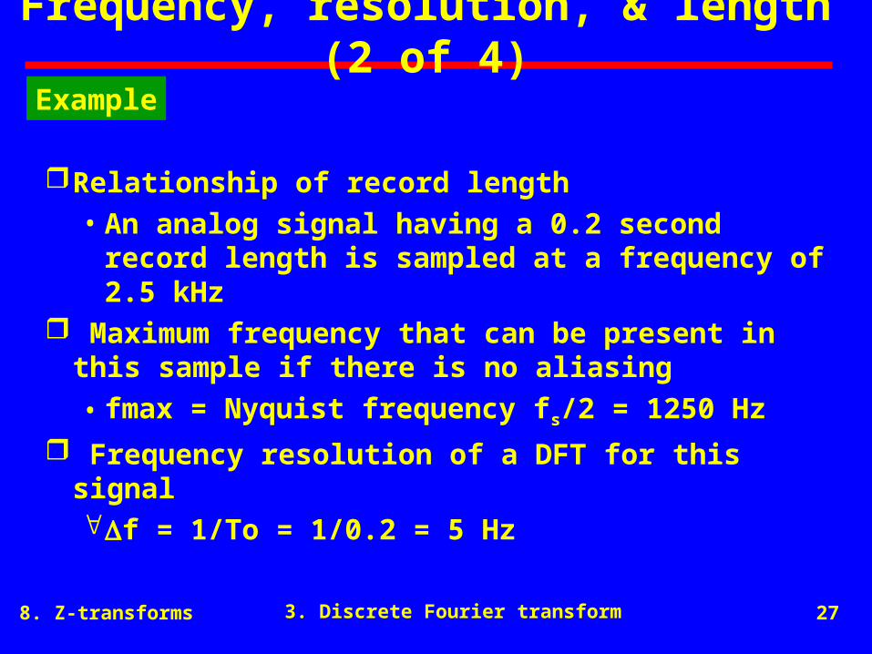
Frequency, resolution, & length (2 of 4)
Relationship of record length• An analog signal having a 0.2 second record
length is sampled at a frequency of 2.5 kHz Maximum frequency that can be present in
this sample if there is no aliasing
• fmax = Nyquist frequency fs/2 = 1250 Hz
Frequency resolution of a DFT for this signalf = 1/To = 1/0.2 = 5 Hz
Example
3. Discrete Fourier transform

8. Z-transforms 28
Frequency, resolution, & length (3 of 4)
Record length• N = To/T = 0.2/(1/2500) = 500 samples
Frequencies present• f = 0, 5, 10, … , 1250, -1245, -1240, … , -5
Example (continued)
3. Discrete Fourier transform

8. Z-transforms 29
Frequency, resolution, & length (4 of 4)
N T To f fmax
N 2T 2 To 0.5 f 0.5 fmax
2N 0.5 T To f 2 fmax
2N T 2 To 0.5 f fmax
Effect of changing numbers
3. Discrete Fourier transform

8. Z-transforms 30
Linear convolution (1 of 7)
h[n]x[n] y[n]
y[n] are determined by convolving x[n] and h[n]
Determining y[n] from x[n] and h[n]
3. Discrete Fourier transform

8. Z-transforms 31
Convolution by multiplication
Introduction to Signal Processing
Sophacles J. Orfanidis page 147
Introduction to Signal Processing
Sophacles J. Orfanidis page 147
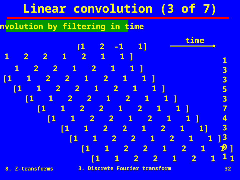
Linear convolution (2 of 7)
h[n] = [1 2 -1 1]x[n] = [1 1 2 1 2 2 1 1 ]y[n] = [1 3 3 5 3 7 4 3 3 0 1]
11=4+8-1
1 1 2 1 2 2 1 11 2 -1 1
1 1 2 1 2 2 1 1 2 2 4 2 4 4 2 2 -1 -1 -2 -1 -2 -2 -1 -1 1 1 2 1 2 2 1 1
1 3 3 5 3 7 4 3 3 0 1
3. Discrete Fourier transform
8. Z-transforms 32
Linear convolution (3 of 7)
[1 2 -1 1][1 1 2 2 1 2 1 1 ] 1
3353743301
[1 1 2 2 1 2 1 1 ][1 1 2 2 1 2 1 1 ]
[1 1 2 2 1 2 1 1 ][1 1 2 2 1 2 1 1 ]
[1 1 2 2 1 2 1 1 ][1 1 2 2 1 2 1 1 ]
[1 1 2 2 1 2 1 1][1 1 2 2 1 2 1 1 ]
[1 1 2 2 1 2 1 1 ][1 1 2 2 1 2 1 1 ]
time
Convolution by filtering in time
3. Discrete Fourier transform

8. Z-transforms 33
Linear convolution (4 of 7)
[1 1 2 1 2 2 1 1 ][1 -1 2 1] 1
3353743301
[1 -1 2 1][1 -1 2 1]
[1 -1 2 1][1 -1 2 1]
[1 -1 2 1][1 -1 2 1]
[1 -1 2 1][1 -1 2 1]
[1 -1 2 1][1 -1 2 1]
filter slideConvolution by sliding filter
3. Discrete Fourier transform

8. Z-transforms 34
Linear convolution (5 of 7)
h[n] = [1 2 -1 1] x[n] = [1 1 2 1 2 2 1 1 ]
Need to have sequences of same length, and length needs to be 4 + 8 -1 = 11 to avoid circular convolution
h[n] = [1 2 -1 1 0 0 0 0 0 0 0 0 0 0 0 0] x[n] = [1 1 2 1 2 2 1 1 0 0 0 0 0 0 0 0]
Convolution by DFT
3. Discrete Fourier transform

8. Z-transforms 35
Linear convolution (6 of 7)
X[k] = 11 1.3244 - 7.6583j-1.7071 - 0.2929j 1.2168 - 0.8210j - j-0.6310 - 0.5784j-0.2929 + 1.7071j 2.0898 + 0.5843j 1 2.0898 - 0.5843j-0.2929 - 1.7071j-0.6310 + 0.5784j + j 1.2168 + 0.8210j-1.7071 + 0.2929j 1.3244 + 7.6583j
H[k] = 3 2.5233 - 0.9821j 1.7071 - 1.1213j 1.5486 - 0.7580j 2 - j 1.8656 - 2.1722j 0.2929 - 3.1213j-1.9375 - 2.3964j-3-1.9375 + 2.3964j 0.2929 + 3.1213j 1.8656 + 2.1722j 2 + j 1.5486 + 0.7580j 1.7071 + 1.1213j 2.5233 + 0.9821j
Y[k]=X[k] H[k] = 33-4.1796 - 20.6253j-3.2426 + 1.4142j 1.2620 - 2.1937j -1 - 2j-2.4335 + 0.2916j 5.2426 + 1.4141j-2.6488 - 6.1400j-3-2.6488 + 6.1400j 5.2426 - 1.4141j-2.4335 - 0.2916j-1 + 2j 1.2620 + 2.1937j-3.2426 - 1.4142j-4.1796 +20.6253j
y[n]=1335 374330100000
3. Discrete Fourier transform

8. Z-transforms 36
Linear convolution (7 of 7)
MATLAB code for convolution by DFT
x = [1,1,2,1,2,2,1,1,0,0,0,0,0,0,0,0]h = [1,2,-1,1,0,0,0,0,0,0,0,0,0,0,0,0]X = fft(x)H = fft(h)Y = X.*Hy = ifft(Y)
Convolution by DFT (continued)
3. Discrete Fourier transform

8. Z-transforms 37
Circular convolution (1 of 4)
yc[n] = x[m] h[ <n-m>N]m=0
N-1
x[n] = [1 1 2 0], h[n] = [1 2 -1 1]
yc[0] = [1 1 2 0] [ 1 1 -1 2] = 0yc[1] = [1 1 2 0] [ 2 1 1 -1] = 5yc[2] = [1 1 2 0] [-1 2 1 1] = 3yc[3] = [1 1 2 0] [ 1 -1 2 1] = 4
Definition and example
3. Discrete Fourier transform

8. Z-transforms 38
Circular convolution (2 of 4)
yc[0]yc[1]yc[2]...yc[N-1]
h[0] h[N-1] h[N-2] … h[1]h[1] h[0] h[N-1] … h[2]h[2] h[1] h[0] … h[3]. . . … .. . . … .. . . … .h[N-1] h[N-2] h[N-3] … h[0]
x[0]x[1]x[2]...x[N-1]
=
Matrix format
3. Discrete Fourier transform
8. Z-transforms 39
Circular convolution (3 of 4)
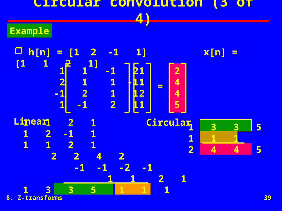
h[n] = [1 2 -1 1] x[n] = [1 1 2 1]
1 1 -1 2 2 1 1 -1-1 2 1 1 1 -1 2 1
1121
2445
1 1 2 11 2 -1 11 1 2 1 2 2 4 2 -1 -1 -2 -1 1 1 2 11 3 3 5 1 1 1
=
Linear Circular 1 3 3 51 1 12 4 4 5
Example
8. Z-transforms 40
Circular convolution (4 of 4)
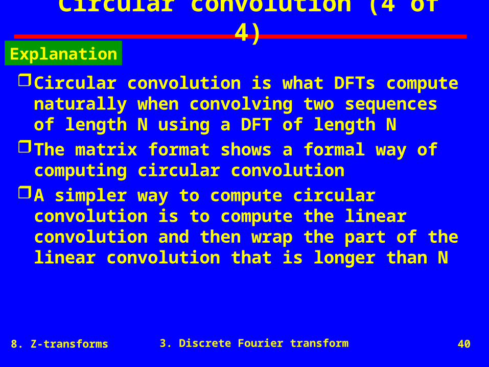
Circular convolution is what DFTs compute naturally when convolving two sequences of length N using a DFT of length N
The matrix format shows a formal way of computing circular convolution
A simpler way to compute circular convolution is to compute the linear convolution and then wrap the part of the linear convolution that is longer than N
Explanation
3. Discrete Fourier transform
8. Z-transforms 41
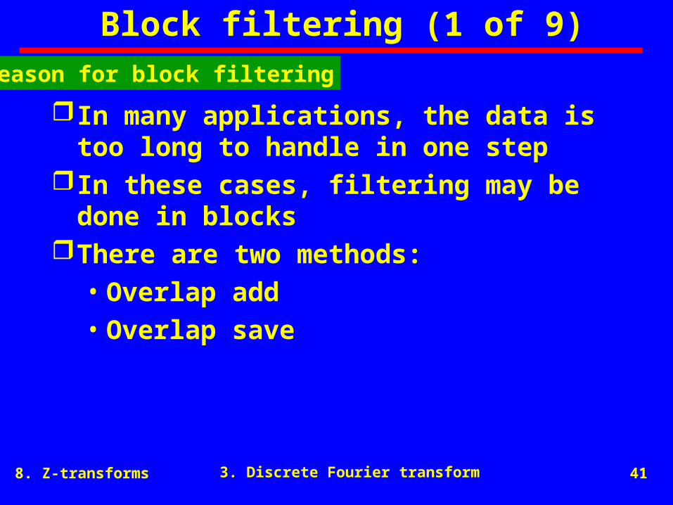
Block filtering (1 of 9)
In many applications, the data is too long to handle in one step
In these cases, filtering may be done in blocks
There are two methods:• Overlap add• Overlap save
Reason for block filtering
3. Discrete Fourier transform
8. Z-transforms 42
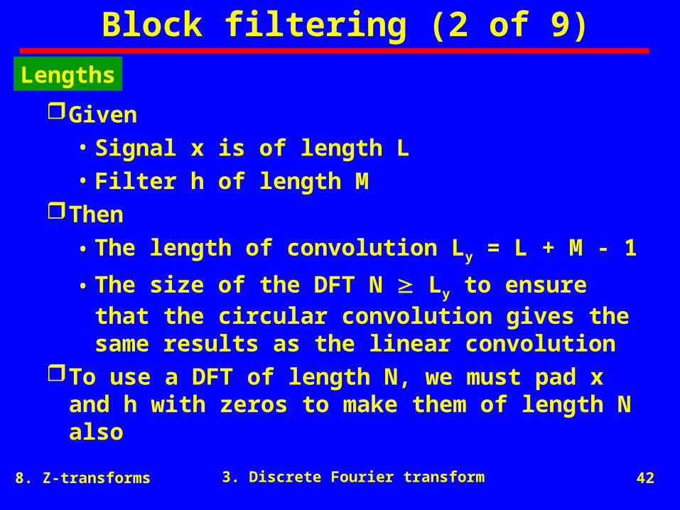
Block filtering (2 of 9)
Given• Signal x is of length L• Filter h of length M
Then
• The length of convolution Ly = L + M - 1
• The size of the DFT N Ly to ensure that the circular convolution gives the same results as the linear convolution
To use a DFT of length N, we must pad x and h with zeros to make them of length N also
Lengths
3. Discrete Fourier transform

8. Z-transforms 43
Block filtering (3 of 9)Overlap add
block xo block x1 block x2
L M
L M
L M
yo =
y1 =
y2 =
x =
L L L
ytemp
ytemp
ytemp
n=0 n=L n=2L n=3L
3. Discrete Fourier transform

8. Z-transforms 44
Block filtering (4 of 9)
h[n] = [1 2 -1 1] x[n] = [1 1 2 1 2 2 1 1 ]y[n] = [1 3 3 5 3 7 4 3 3 0 1]
x1[n] = [1 1 2], x2[n] = [1 2 2], x3[n] = [1 1]
1 2 -1 11 1 21 3 3 4 -1 2
1 2 -1 11 2 21 4 5 3 0 2
1 2 -1 11 11 3 1 0 1
1 3 3 4 -1 2 1 4 5 3 0 2 1 3 1 0 11 3 3 5 3 7 4 3 3 0 1
Divide input sequence into 3 parts
Overlap-add (continued)
3. Discrete Fourier transform

8. Z-transforms 45
Block filtering (5 of 9)
x = [1,1, 2, 0,0,0,0,0]h = [1,2,-1,1, 0,0,0,0]X = fft(x)H = fft(h)Y = X.*Hy = ifft(Y)
y[n] = [1 3 3 4 -1 2 0 0]
MATLAB code for convolution by DFT
3. Discrete Fourier transform

8. Z-transforms 46
Block filtering (6 of 9)Overlap save
x = M MM
block xo block x1 block x2 block x3
N-MM
N-MM
N-MM
N-MM
yo=
y1=
y2=
y3=
n=0 n=N n=2N n=3N3. Discrete Fourier transform

8. Z-transforms 47
Block filtering (7 of 9)
h[n] = [1 -1 -1 1]x[n] = [1,1,1,1,3,3,3,3,1,1,1,2,2,2,2,1,1,1,1]y[n] = [1,0,-1,0,2,0,-2,0,-2,0,2,1,0,-1,0,-1,0,1,0,-1,0,1]
Divide input sequence into sequences of length 8that overlap by 3
But first, attach 8-3 = 5 zeros to front of sequence
x[n] = [0,0,0,0,0,1,1,1,1,3,3,3,3,1,1,1,2,2,2,2,1,1,1,1]
Overlap save (continued)
3. Discrete Fourier transform
8. Z-transforms 48
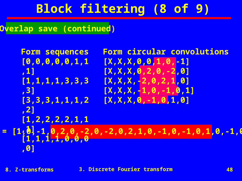
Block filtering (8 of 9)
Form sequences[0,0,0,0,0,1,1,1][1,1,1,1,3,3,3,3][3,3,3,1,1,1,2,2][1,2,2,2,2,1,1,1][1,1,1,1,0,0,0,0]
Form circular convolutions[X,X,X,0,0,1,0,-1][X,X,X,0,2,0,-2,0][X,X,X,-2,0,2,1,0][X,X,X,-1,0,-1,0,1][X,X,X,0,-1,0,1,0]
y[n] = [1,0,-1,0,2,0,-2,0,-2,0,2,1,0,-1,0,-1,0,1,0,-1,0,1]
Overlap save (continued)
3. Discrete Fourier transform
8. Z-transforms 49
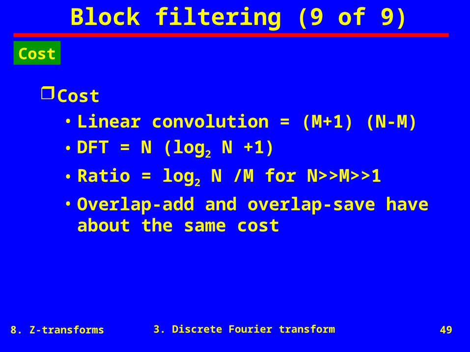
Block filtering (9 of 9)
Cost• Linear convolution = (M+1) (N-M)
• DFT = N (log2 N +1)
• Ratio = log2 N /M for N>>M>>1
• Overlap-add and overlap-save have about the same cost
Cost
3. Discrete Fourier transform

8. Z-transforms 50
Filtering (1 of 11)
Filter -- A filter is an algorithm that converts in input sequence into an output sequence
Linear, constant-coefficient difference equation (LCCDE)
y[n] = b[k] x[n-k] - a[k] y[n-k]k=0
q
k=1
p
Definition
3. Discrete Fourier transform

8. Z-transforms 51
Filtering (2 of 11)
Impulse response, h[n] -- h[n] is found by solving the LCDDE for x[n] = [n]
Impulse response
3. Discrete Fourier transform

8. Z-transforms 52
Filtering (3 of 11)
Infinite impulse response (IIR) filter -- A FIR is a filter in which the length of h[n] is infinite. It corresponds to an LCCDE in which not all the values of a[n-k] are zero• y[n] = -0.5 y[n-1] + 0.5 x[n]
IIR advantages• Useful for implementing analog filters in
digital format• Sometimes has fewer coefficients
IIR
3. Discrete Fourier transform

8. Z-transforms 53
Filtering (4 of 11)
Finite impulse response (FIR) filter -- A FIR is a filter in which the length of h[n] is finite. It corresponds to an LCCDE in which all the values of a[n-k] are zero• y[n] = 0.25 x[n] + 0.50 x[n-1] + 0.25 x[n-2]
FIR advantages• Simple• Always stable• Linear phase
FIR
3. Discrete Fourier transform
8. Z-transforms 54
Filtering (5 of 11)
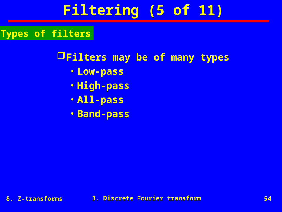
Filters may be of many types• Low-pass• High-pass• All-pass• Band-pass
Types of filters
3. Discrete Fourier transform

8. Z-transforms 55
Filtering (6 of 11)
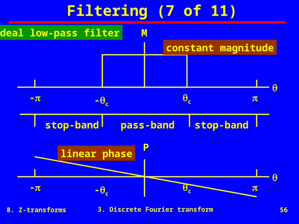
Ideal filter• Magnitude -- constant across pass-band• Phase -- linear across pass-band
Reason for ideal filter• The envelope of a signal will not be
distorted when passing through a filter with linear phase
Ideal filter
3. Discrete Fourier transform
8. Z-transforms 56
Filtering (7 of 11)
c-c
M
stop-band stop-bandpass-band
-
c-c
-
ideal low-pass filter
constant magnitude
linear phaseP
3. Discrete Fourier transform
8. Z-transforms 57
Filtering (8 of 11)
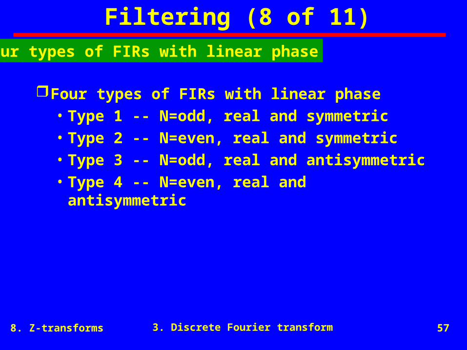
Four types of FIRs with linear phase• Type 1 -- N=odd, real and symmetric• Type 2 -- N=even, real and symmetric• Type 3 -- N=odd, real and antisymmetric• Type 4 -- N=even, real and antisymmetric
Four types of FIRs with linear phase
3. Discrete Fourier transform

8. Z-transforms 58
Filtering (9 of 11)
Linear phase -- An LTI system has linear phase if • H(e j ) = |H (e j )| e -j
Generalized linear phase -- An LTI has generalized linear phase if • H(e j ) = |H (e j )| e -j ( - )
Linear phase
3. Discrete Fourier transform

8. Z-transforms 59
Filtering (10 of 11)
type 1 type 2
type 3 type 4
Types (continued)
3. Discrete Fourier transform
8. Z-transforms 60
Filtering (11 of 11)
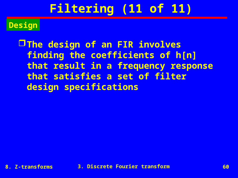
The design of an FIR involves finding the coefficients of h[n] that result in a frequency response that satisfies a set of filter design specifications
Design
3. Discrete Fourier transform
8. Z-transforms 61
Windowing (1 of 4)
Windowing -- The process of reducing the length of the original signal because we can take DFTs of unlimited size
Purpose• Reduces the frequency resolution• Introduces spurious frequency
components into the spectrum -- called frequency leakage
Equation
• xL [n] = x[n] w[n]
Definitions
3. Discrete Fourier transform
8. Z-transforms 62
Windowing (2 of 4)
0 5 10 15 20 25 30 350
0.1
0.2
0.3
0.4
0.5
0.6
0.7
0.8
0.9
1
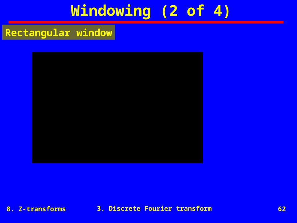
Rectangular window
3. Discrete Fourier transform

8. Z-transforms 63
Windowing (3 of 4)
0 5 10 15 20 25 30 35 400
0.1
0.2
0.3
0.4
0.5
0.6
0.7
0.8
0.9
1
Hanning window
3. Discrete Fourier transform

8. Z-transforms 64
Windowing (4 of 4)
0 5 10 15 20 25 30 350
2
4
6
8
10
12
14
16
0 5 10 15 20 25 30 350
1
2
3
4
5
6
7
8
9
Rectangular window withsidelobe at -13 dB
Hamming window withsidelobe at -40 dB
Comparison of effect of rectangular & Hamming windows
3. Discrete Fourier transform

8. Z-transforms 65
4. Power spectral density
Power spectrum (PS)Power spectral density (PSD)ExperimentUse of PSDEffect of linear system on PSD
4. Power spectral density

8. Z-transforms 66
Power spectrum (PS)
x2 = 1/2 Cn C*n
n=1
The mean square value of a periodic time function is the sum of the mean square value of the individual harmonic components present
The power spectrum G(fn) = 1/2 Cn C*n is the contribution to the mean square error in the frequency interval f
x2 = G(fn) n=1

8. Z-transforms 67
Power spectral density (PSD)
The power spectral density S(fn) is the power spectrum divided by the frequency interval f
S(fn) = G(fn) / f
x2 = S(fn) f n=1
4. Power spectral density

8. Z-transforms 68
Experiment
shaker accelerometer amplifier filterRMSmeter
f
420-580 Hz480-520 Hz495-505 Hz
f
160 Hz40 Hz10 Hz
meter
8g4g2g
G(fn)
64g2
16g2
4g2
S(fn)/ f
0.40g2/Hz0.40g2/Hz0.40g2/Hz
Theory of Vibration with Applications, William T. Thompson
4. Power spectral density
8. Z-transforms 69
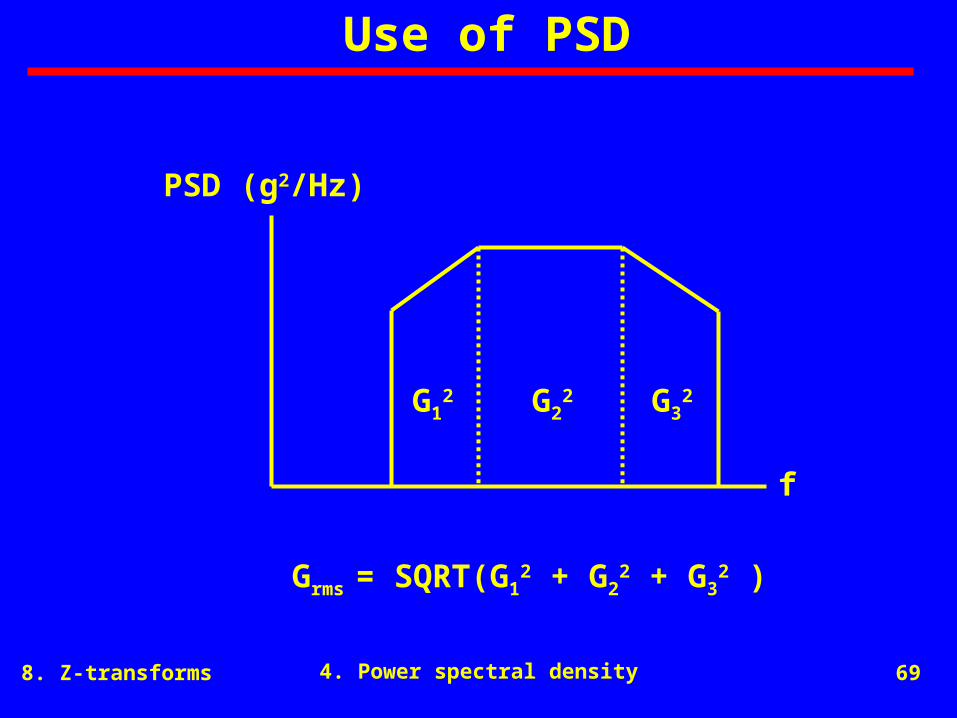
Use of PSD
G12 G2
2 G32
Grms = SQRT(G12 + G2
2 + G32 )
f
PSD (g2/Hz)
4. Power spectral density
8. Z-transforms 70
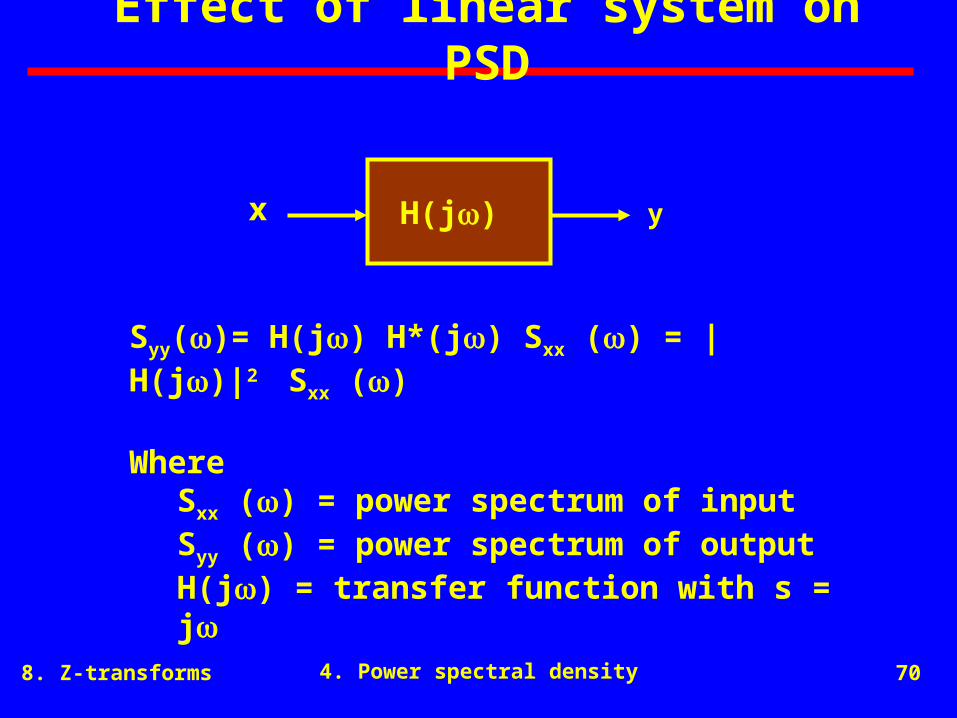
Effect of linear system on PSD
H(j)
Syy()= H(j) H*(j) Sxx () = |H(j)|2 Sxx ()
Where Sxx () = power spectrum of inputSyy () = power spectrum of outputH(j) = transfer function with s = j
x y
4. Power spectral density