8.044 Lecture NotesChapter 2: Probability for 8.044

Lecturer: McGreevy

Contents

2.1 One random variable . . . . . . . . . . . . . . . . . . . . . . . . . . . . . . . 2-1

2.1.1 A trick for doing the gaussian integral by squaring it . . . . . . . . . 2-11

2.1.2 A trick for evaluating moments of the gaussian distribution . . . . . . 2-11

2.2 Two random variables . . . . . . . . . . . . . . . . . . . . . . . . . . . . . . 2-16

2.3 Functions of a random variable . . . . . . . . . . . . . . . . . . . . . . . . . 2-28

2.4 Sums of statistically-independent random variables . . . . . . . . . . . . . . 2-32

2.5 Epilog: an alternate derivation of the Poisson distribution . . . . . . . . . . 2-47

2.5.1 Random walk in one dimension . . . . . . . . . . . . . . . . . . . . . 2-47

2.5.2 From binomial to Poisson . . . . . . . . . . . . . . . . . . . . . . . . 2-48

Reading: Notes by Prof. Greytak

How we count in 8.044: first one random variable, then two random variables, then 1024

random variables.

2.1 One random variable

A random variable (RV) is a quantity whose value can’t be predicted (with certainty)given what we know. We have limited knowledge, in the form of a probability distribution.

2-1

Two basic sources of uncertainty (and hence RVs) in physics:

1. quantum mechanics (8.04)

Even when the state of the system is completely specified, some measurement outcomescan’t be predicted with certainty. Hence they are RVs.

2. ignorance (8.044)

This happens when we have insufficient information to fully specify the state of thesystem, e.g. because there are just too many bits for us to keep track of. Suppose weknow P, V, T, E, S of a cylinder of gas – this determines the macrostate. ~x, ~p of the1024 molecules are not specified by this. So we will use RVs to describe the microstate.

Types of RVs:

• continuous: (e.g. position or velocity of gas atoms) real numbers.

• discrete: (e.g. number of gas atoms in the room) integers.

• mixed: both continuous and discrete components (e.g. energy spectrum of H atom hasdiscrete boundstate energies below a continuum)

2-2

Probability theory can be based on an ensemble of similarly prepared systems.

e.g. many copies of a cylinder of gas, all with the same P, V, T, E, S.all determined (i.e. macroscopic) are the same.

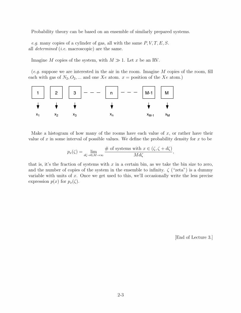
Imagine M copies of the system, with M � 1. Let x be an RV.

(e.g. suppose we are interested in the air in the room. Imagine M copies of the room, filleach with gas of N2, O2, ... and one Xe atom. x = position of the Xe atom.)

1

x1

2

x2

3

x3

n

xn

M-1

xM-1

M

xM

Make a histogram of how many of the rooms have each value of x, or rather have theirvalue of x in some interval of possible values. We define the probability density for x to be

px(ζ) = limdζ→0,M→∞

# of systems with x ∈ (ζ, ζ + dζ)

Mdζ,

that is, it’s the fraction of systems with x in a certain bin, as we take the bin size to zero,and the number of copies of the system in the ensemble to infinity. ζ (“zeta”) is a dummyvariable with units of x. Once we get used to this, we’ll occasionally write the less preciseexpression p(x) for px(ζ).

[End of Lecture 3.]

2-3

A simple example of assembling a probability distrbution: shoot arrows at a target.

x is horizontal displacement from bullseye (in some units, say millimeters).

Make a histogram of values of x: divide up the possible locations into bins of size dζ, andcount how many times the arrow has an x-position in each bin. Shoot M arrows.

In these plots, I am just showing raw numbers of hits in each bin on the vertical axis, andI am fixing the bin size. In the three plots I’ve taken M = 500, 5000, 50000.

Claim: [histogram]M→∞,dζ→0−→ [smooth distribution]

2-4

Properties of px:

• Prob(x between ζ and ζ + dζ) = px(ζ)dζ. (So the probability of hitting any particularpoint exactly is zero if p is smooth. But see below about delta functions.)

• p is real

• px(ζ) ≥ 0.

• Prob(x ∈ (a, b)) =∫ bapx(ζ)dζ

• The fact that the arrow always ends up somewhere means that the distribution isnormalized:∫∞−∞ px(ζ)dζ = 1.

• the units of px are 1units of x

. (e.g. 1 is dimensionless.)

2-5

The probability density is a way of packaging what we do know about a RV. Anotherconvenient package for the same info is:

Cumulative probability

P (ζ) ≡ Prob(x < ζ) =

∫ ζ

−∞dζ ′px(ζ

′).

(Note the serif on the capital P .) To get back the probability density:

px(ζ) =d

dζP (ζ).

The question we have to answer in this chapter of the course is: “Given p or P , what canwe learn?” How to determine p is the subject of 8.04 and the whole rest of 8.044. So in thenext few lectures, we’ll have to cope with Probability Densities from Outer Space, i.e. I’mnot going to explain where the come from.

2-6

Example of a discrete density:

Consider an atom bounces around in a cavity with a hole.

Prob(atom escapes after a given bounce) = a

for some small constant a.

p(n) ≡ Prob(atom escapes after n bounces)

is a probability, not a density. n = 0, 1, 2...

p(n) = (1− a)n︸ ︷︷ ︸ × a︸︷︷︸prob that it failed to escape n times and then escaped on the nth

Repackage:

pn(ζ) =∞∑n=0

p(n)δ(ζ − n) =∞∑n=0

(1− a)naδ(ζ − n).

(δ(x) here is the Dirac delta function, which has the propertythat it vanishes for any x 6= 0 but integrates to 1 around anyneighborhood of x = 0.) The point of this interlude is that allmanipulations can be done in the same formalism for discrete and continuum cases, we don’tneed to write separate equations for the discrete case.

(Note convention for sketching δ-functions.)

P always asymptotes to 1, since∫ALL

p = 1.

Check normalization:∑∞

n=0 a(1 − a)n = a 11−(1−a)

. You should get used to checking thenormalization whenever anyone gives you an alleged probability distribution. Trust no one!

This is called a ‘geometric’ or ‘Bose-Einstein’ distribution.

2-7

What to do with a probability density? p(x) is a lot of information. Here’s how to extractthe bits which are usually most useful.

Averages

Mean: 〈x〉 ≡∫ ∞−∞

xp(x)dx

Mean square: 〈x2〉 ≡∫ ∞−∞

x2p(x)dx

nth Moment: 〈xn〉 ≡∫ ∞−∞

xnp(x)dx

〈f(x)〉 ≡∫ ∞−∞

f(ζ)px(ζ)dζ =

∫ ∞−∞

f(x)p(x)dx

Meaning: make a histogram of f(x) instead of a histogram of x. What is the mean of thishistogram?

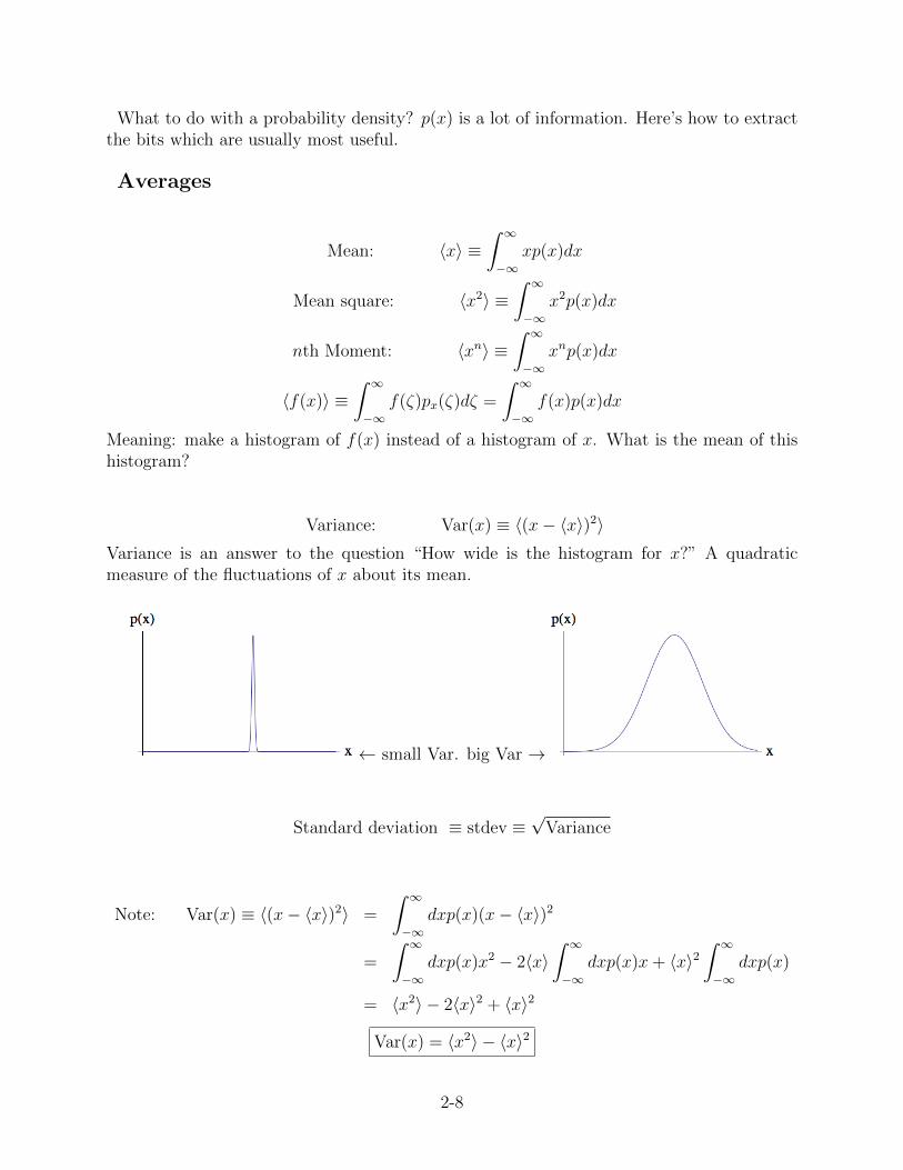
Variance: Var(x) ≡ 〈(x− 〈x〉)2〉Variance is an answer to the question “How wide is the histogram for x?” A quadraticmeasure of the fluctuations of x about its mean.

← small Var. big Var →

Standard deviation ≡ stdev ≡√

Variance

Note: Var(x) ≡ 〈(x− 〈x〉)2〉 =

∫ ∞−∞

dxp(x)(x− 〈x〉)2

=

∫ ∞−∞

dxp(x)x2 − 2〈x〉∫ ∞−∞

dxp(x)x+ 〈x〉2∫ ∞−∞

dxp(x)

= 〈x2〉 − 2〈x〉2 + 〈x〉2

Var(x) = 〈x2〉 − 〈x〉2

2-8

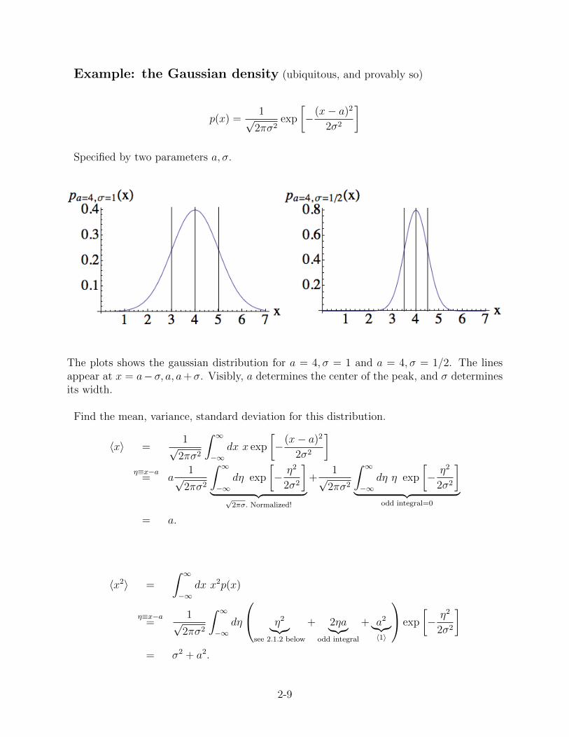
Example: the Gaussian density (ubiquitous, and provably so)

p(x) =1√

2πσ2exp

[−(x− a)2

2σ2

]

Specified by two parameters a, σ.

The plots shows the gaussian distribution for a = 4, σ = 1 and a = 4, σ = 1/2. The linesappear at x = a−σ, a, a+σ. Visibly, a determines the center of the peak, and σ determinesits width.

Find the mean, variance, standard deviation for this distribution.

〈x〉 =1√

2πσ2

∫ ∞−∞

dx x exp

[−(x− a)2

2σ2

]η≡x−a

= a1√

2πσ2

∫ ∞−∞

dη exp

[− η2

2σ2

]︸ ︷︷ ︸√

2πσ. Normalized!

+1√

2πσ2

∫ ∞−∞

dη η exp

[− η2

2σ2

]︸ ︷︷ ︸

odd integral=0

= a.

〈x2〉 =

∫ ∞−∞

dx x2p(x)

η≡x−a=

1√2πσ2

∫ ∞−∞

dη

η2︸︷︷︸see 2.1.2 below

+ 2ηa︸︷︷︸odd integral

+ a2︸︷︷︸〈1〉

exp

[− η2

2σ2

]= σ2 + a2.

2-9

Gaussian density, cont’d

Please see Prof. Greytak’s probability notes (page 13), and the subsections below, and yourrecitation instructors, for more on how to do the integrals. The conclusion here is that forthe gaussian distribution,

Var(x) = σ2, stdev(x) = σ.

Cumulative probability:

P (x) =1√

2πσ2

∫ x

−∞dζ e−

(ζ−a)2

2σ2 .

This is an example to get us comfortable with the notation, and it’s an example whicharises over and over. Soon: why it arises over and over (Central Limit Theorem).

2-10

2.1.1 A trick for doing the gaussian integral by squaring it

Consider the distribution

P (x1, x2) = C2e−x212s2 e−

x222s2

describing two statistically independent random variables on the real line, each of which isgoverned by the Gaussian distribution. What is C?

1 = C2

∫dx1dx2e

− x212s2 e−

x222s2 = C2

∫rdrdθe−

r2

2s2 = 2πC2

∫ ∞0

rdre−r2

2s2

This is the square of a single gaussian integral. Let u = r2

2s2, rdr = s2du:

1 = 2πC2s2

∫ ∞0

due−u = 2πC2s2(−e−u

)|∞0 = 2πC2s2

2.1.2 A trick for evaluating moments of the gaussian distribution

The key formula to use is: for any X ,∫ ∞−∞

dη η2e−Xη2

= − ∂

∂X

∫ ∞−∞

dη e−Xη2

.

2-11

Another example: Poisson density

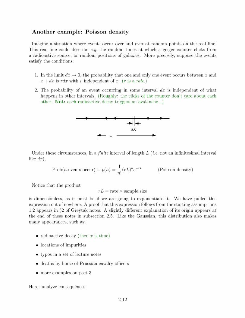
Imagine a situation where events occur over and over at random points on the real line.This real line could describe e.g. the random times at which a geiger counter clicks froma radioactive source, or random positions of galaxies. More precisely, suppose the eventssatisfy the conditions:

1. In the limit dx→ 0, the probability that one and only one event occurs between x andx+ dx is rdx with r independent of x. (r is a rate.)

2. The probability of an event occurring in some interval dx is independent of whathappens in other intervals. (Roughly: the clicks of the counter don’t care about eachother. Not: each radioactive decay triggers an avalanche...)

Under these circumstances, in a finite interval of length L (i.e. not an infinitesimal intervallike dx),

Prob(n events occur) ≡ p(n) =1

n!(rL)ne−rL (Poisson density)

Notice that the productrL = rate× sample size

is dimensionless, as it must be if we are going to exponentiate it. We have pulled thisexpression out of nowhere. A proof that this expression follows from the starting assumptions1,2 appears in §2 of Greytak notes. A slightly different explanation of its origin appears atthe end of these notes in subsection 2.5. Like the Gaussian, this distribution also makesmany appearances, such as:

• radioactive decay (then x is time)

• locations of impurities

• typos in a set of lecture notes

• deaths by horse of Prussian cavalry officers

• more examples on pset 3

Here: analyze consequences.

2-12

Poisson density, cont’d

Rewrite as a continuous density:

p(y) =∞∑n=0

p(n)δ(y − n).

To do: check normalization, compute mean and variance.

Normalize: 1!

=

∫ ∞−∞

dyp(y) =

∫ ∞−∞

dy

∞∑n=0

p(n)δ(y − n)

=∞∑n=0

p(n)

(∫ ∞−∞

dyδ(y − n)

)︸ ︷︷ ︸

=1

= e−rL∞∑n=0

1

n!(rL)n = e−rLerL = 1.

〈n〉 =

∫ ∞−∞

dyp(y)y =

∫ ∞−∞

dy∞∑n=0

p(n)δ(y − n)y =∞∑n=0

np(n)

= e−rL∞∑

n = 0︸ ︷︷ ︸n = 0 doesn’t contribute

n

n!(rL)n = e−rLrL

∞∑n=1

1

(n− 1)!(rL)n−1

︸ ︷︷ ︸erL

= rL.

or:∂

∂r

[erL =

∞∑n=0

1

n!(rL)n

]

=⇒ LerL =∞∑n=0

n

n!(rL)n︸ ︷︷ ︸

what we want

1

r.

2-13

Poisson density, cont’d

〈n2〉 = ... =∞∑n=0

n2p(n) = ... = (rL)(rL+ 1).

Differentiate erL twice. See Greytak notes for more of this.

=⇒ Var(n) = 〈n2〉 − 〈n〉2 = rL.

rL = 〈n〉.

The Poisson density has the same mean and variance. The std deviation is√rL.

Note that only the (dimensionless) combination rL appears in the distribution itself.

Rewrite:

p(n) =1

n!〈n〉ne−〈n〉.

Getting used to this abuse of notation is useful: n is the random variable.〈n〉 is a number.

2-14

rL = 〈n〉 = 1/2

rL = 〈n〉 = 3

rL = 〈n〉 = 25

As we increase rL the (envelope of the) distribution is visibly turning into a gaussian with〈n〉 = rL, Var(n) = rL, stdev = σ =

√rL. (This is an example of a more general phe-

nomenon which we’ll discuss soon, in 2.3.)

2-15

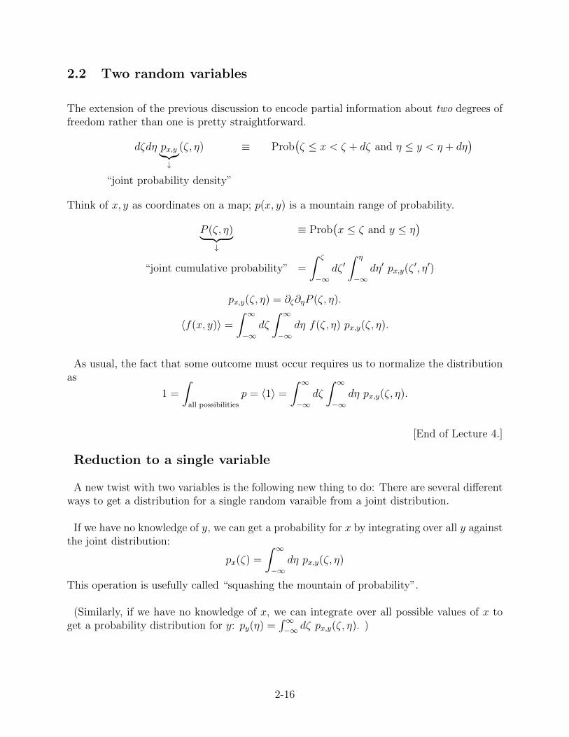
2.2 Two random variables

The extension of the previous discussion to encode partial information about two degrees offreedom rather than one is pretty straightforward.

dζdη px,y︸︷︷︸↓

(ζ, η) ≡ Prob(ζ ≤ x < ζ + dζ and η ≤ y < η + dη

)“joint probability density”

Think of x, y as coordinates on a map; p(x, y) is a mountain range of probability.

P (ζ, η)︸ ︷︷ ︸↓

≡ Prob(x ≤ ζ and y ≤ η

)“joint cumulative probability” =

∫ ζ

−∞dζ ′∫ η

−∞dη′ px,y(ζ

′, η′)

px,y(ζ, η) = ∂ζ∂ηP (ζ, η).

〈f(x, y)〉 =

∫ ∞−∞

dζ

∫ ∞−∞

dη f(ζ, η) px,y(ζ, η).

As usual, the fact that some outcome must occur requires us to normalize the distributionas

1 =

∫all possibilities

p = 〈1〉 =

∫ ∞−∞

dζ

∫ ∞−∞

dη px,y(ζ, η).

[End of Lecture 4.]

Reduction to a single variable

A new twist with two variables is the following new thing to do: There are several differentways to get a distribution for a single random varaible from a joint distribution.

If we have no knowledge of y, we can get a probability for x by integrating over all y againstthe joint distribution:

px(ζ) =

∫ ∞−∞

dη px,y(ζ, η)

This operation is usefully called “squashing the mountain of probability”.

(Similarly, if we have no knowledge of x, we can integrate over all possible values of x toget a probability distribution for y: py(η) =

∫∞−∞ dζ px,y(ζ, η). )

2-16

Example: “hockey puck” distribution

top view:

p(x, y) =

1π, for x2 + y2 ≤ 1

0, for x2 + y2 > 1

.

p(x) =

∫ ∞−∞

dy p(x, y) =

√1−x2∫

−√

1−x2dy 1

π= 2

π

√1− x2, for x ≤ 1

0, for x > 1

2-17

Here is a second way to get a probability distribution for one variable from a joint distri-bution for two. It is a little more delicate.

Conditional probability density

Suppose we do know something about y. For example, suppose we have a probabilitydistribution p(x, y) and suddenly discover a new way to measure the value of y; then we’dlike to know what information that gives us about x:

px(ζ|y)dζ ≡ Prob(ζ ≤ x < ζ + dζ given that η = y

)is a single-variable probability density for x; ζ is a dummy variable as usual. y is a parameterof the distribution px(ζ|y), not a random variable anymore. The operation of forming theconditional probability can be described as “slicing the mountain”: since we are specifyingy, we only care about the possibilities along the slice η = y in the picture.

This means that p(ζ|y) must be proportional to px,y(ζ, y). There is no reason for the latterquantity to be normalized as a distribution for ζ, however:

px,y(ζ, y)︸ ︷︷ ︸a slice: not normalized

= c︸︷︷︸to be determined

px(ζ|y)︸ ︷︷ ︸a normalized prob density for ζ

The condition that px(ζ|y) be normalized determines the constant c. As follows:

∫ ∞−∞

dζpx,y(ζ, y)︸ ︷︷ ︸py(η=y)

= c

∫ ∞−∞

dζpx(ζ|y)︸ ︷︷ ︸=1

=⇒ c = py(η = y).

px,y(ζ, y) = py(η = y)px(ζ|y)

2-18

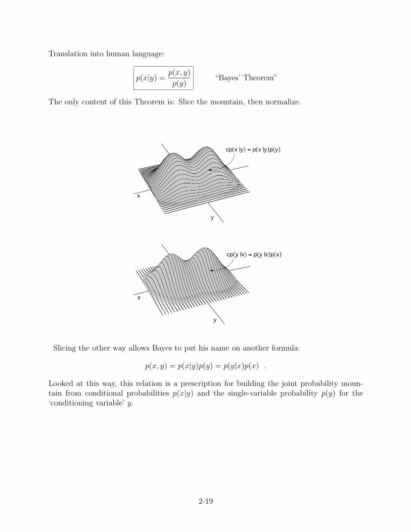
Translation into human language:

p(x|y) =p(x, y)

p(y)“Bayes’ Theorem”

The only content of this Theorem is: Slice the mountain, then normalize.

Slicing the other way allows Bayes to put his name on another formula:

p(x, y) = p(x|y)p(y) = p(y|x)p(x) .

Looked at this way, this relation is a prescription for building the joint probability moun-tain from conditional probabilities p(x|y) and the single-variable probability p(y) for the‘conditioning variable’ y.

2-19

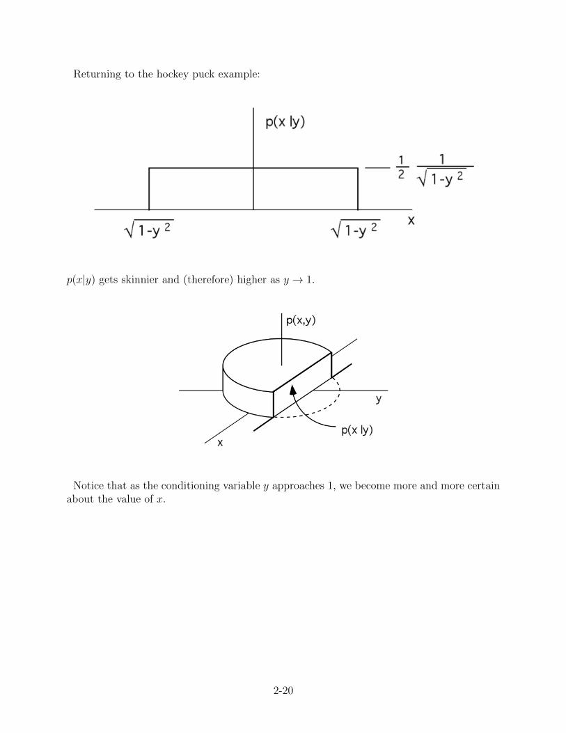
Returning to the hockey puck example:

p(x|y) gets skinnier and (therefore) higher as y → 1.

Notice that as the conditioning variable y approaches 1, we become more and more certainabout the value of x.

2-20

With these defs, we can make a useful characterization of a joint distribution:

Statistical Independence

Two random variables are statistically independent (SI) if the joint distribution factorizes:

px,y(ζ, η) = px(ζ)py(η)

or, equivalently, if

p(x|y) =p(x, y)

p(y)= p(x), independent of y

(in words: the conditional probability for x given y is independent of the choice of y. Tellingme y leaves me as ignorant of x as before.) and

p(y|x) =p(x, y)

p(x)= p(y), independent of x

So: for SI RVs, knowing something about one variable gives no additional information aboutthe other. You are still just as ignorant about the other as you were before you knew anythingabout the first one.

Hockey puck example: x and y are NOT SI.

Example: Deriving the Poisson density.

Now you have all the ingredients necessary to follow the discussion of the derivation ofthe Poisson density in Prof. Greytak’s notes. You have seen a different derivation of thisdistribution in recitation, which is reviewed in the final sub section of these notes (2.5).

2-21

Example: Jointly gaussian random variables

p(v1, v2) =1

2πσ2√

1− ρ2exp[−v

21 − 2ρv1v2 + v2

2

2σ2(1− ρ2)]

v1, v2: random variables. v is for ‘voltage’ as we’ll see later.ρ, σ: parameters specifying the density. They satisfy σ > 0;−1 ≤ ρ ≤ 1.

Start by analyzing the special case ρ = 0:

p(v1, v2) =1√

2πσ2e−

v212σ2

1√2πσ2

e−v222σ2 = p(v1) · p(v2),

a circularly symmetric gaussian mountain. In this case, v1 andv2 are SI, as demonstrated by the last equality above. Slicing agaussian mountain gives gaussian slices.

Now consider ρ 6= 0.

Start by plotting. Contours of constant probability are ellipsesin the (v1, v2) plane:

1

2 1

2

12

v

v

v = vv = −v

ρ = −1 + ε ρ = 0 ρ = 1− ε

2-22

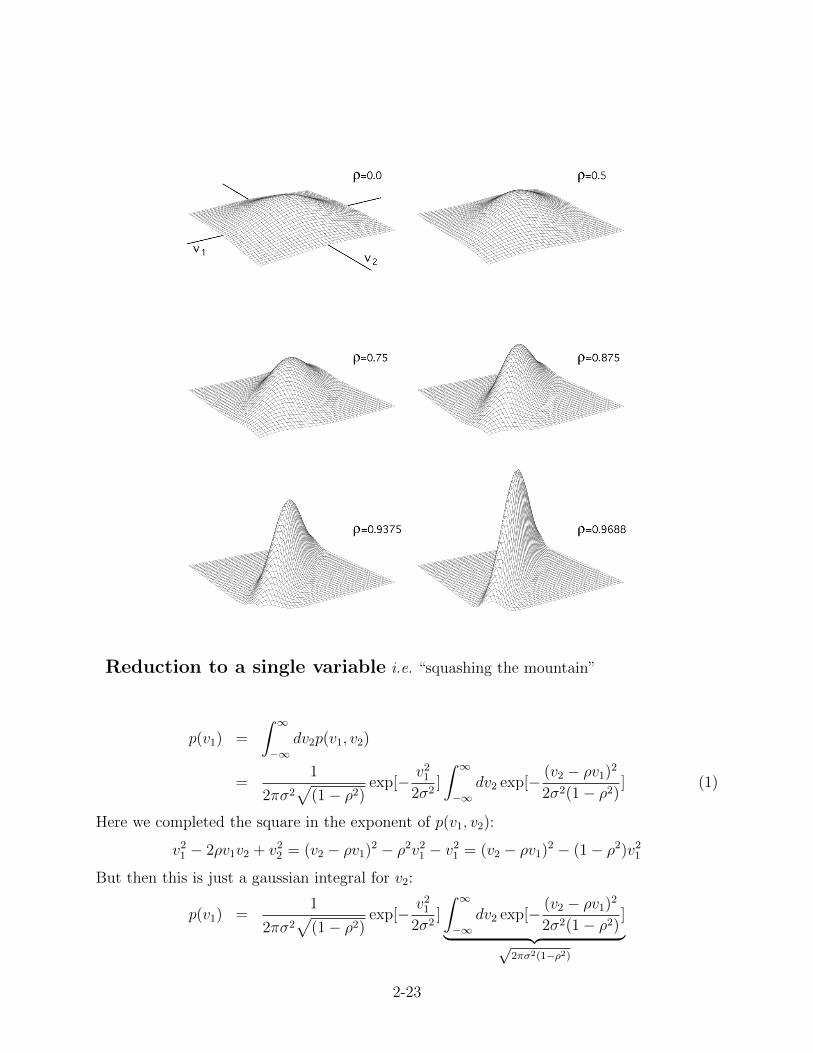
Reduction to a single variable i.e. “squashing the mountain”

p(v1) =

∫ ∞−∞

dv2p(v1, v2)

=1

2πσ2√

(1− ρ2)exp[− v2

1

2σ2]

∫ ∞−∞

dv2 exp[− (v2 − ρv1)2

2σ2(1− ρ2)] (1)

Here we completed the square in the exponent of p(v1, v2):

v21 − 2ρv1v2 + v2

2 = (v2 − ρv1)2 − ρ2v21 − v2

1 = (v2 − ρv1)2 − (1− ρ2)v21

But then this is just a gaussian integral for v2:

p(v1) =1

2πσ2√

(1− ρ2)exp[− v2

1

2σ2]

∫ ∞−∞

dv2 exp[− (v2 − ρv1)2

2σ2(1− ρ2)]︸ ︷︷ ︸√

2πσ2(1−ρ2)

2-23

=1√

2πσ2exp[− v2

1

2σ2] (2)

This is independent of ρ. Similarly for p(v2).

Statistical Independence? The distribution only factorizes if ρ = 0. If ρ 6= 0, not SI.

Information about the correlations between v1 and v2 (i.e. all data about the effect of ρ onthe joint distribution) is lost in the squashing process. This information is hiding in the ...

Conditional probability: (i.e. “slicing the mountain”)

p(v2|v1) =p(v1, v2)

p(v1)

=

√2πσ2

2πσ2√

1− ρ2exp

[−v

21 − 2ρv1v2 + v2

2

2σ2(1− ρ2)+

v21(1− ρ2)

2σ2(1− ρ2)

](3)

But now the same manipulation of completing the square as above shows that this is

p(v2|v1) =1√

2πσ2

1√1− ρ2

exp

[− (v2 − ρv1)2

2σ2(1− ρ2)

](4)

This is a probability density for v2 which is gaussian, with mean ρv1 (remember v1 is aparameter labelling this distribution for the random variable v2), with stdev = σ

√1− ρ2.

1v

v

v = v

1

2

1

1

2

2 v<v > = vρ

Look at the contour plots again. Pick a v1. This determines adistribution for v2 with 〈v2〉v1 = ρv1:

2-24

Plots of p(v2|v1) for various v1:

Note: as ρ→ 1, p(v2|v1)→ δ(v2 − ρv1).

2-25

Correlation function:

≡ 〈v1v2〉 =

∫ ∞−∞

dv1

∫ ∞−∞

dv2 v1v2p(v1, v2)

We could just calculate, but we’ve already done the hard part. Use Bayes here:

〈v1v2〉 =

∫ ∞−∞

dv1

∫ ∞−∞

dv2 v1v2p(v2|v1)p(v1)

〈v1v2〉 =

∫ ∞−∞

dv1v1p(v1)

∫ ∞−∞

dv2 v2p(v2|v1)︸ ︷︷ ︸conditional mean=ρv1

in our joint gaussian example

〈v1v2〉 = ρ

∫ ∞−∞

dv1v21p(v1)︸ ︷︷ ︸

=σ2

= ρσ2.

ρ > 0 : v1, v2 correlatedρ < 0 : v1, v2 anticorrelated

2-26

Whence this probability distribution?

Johnson noise: thermal noise in the voltage across an electric circuit with L,R,C (but nobatteries) at room temperature.

This is an attempt at a random curve with 〈v〉 = 0, 〈v2〉 − 〈v〉2 = σ2, something whichdepends on temperature, but with some excess power at a certain frequency (500 Hz). Tosee this excess power:

Define: v1 ≡ V (t), v2 ≡ V (t+ τ). What do we expect as τ varies?• For large τ : v1, v2 are uncorrelated =⇒ ρ→ 0. Each is gaussian. σ depends on T .• For τ → 0: v1 and v2 are highly correlated: ρ→ 1.• For intermediate τ , they can be (but need not be) anticorrelated:

e.g.:

Different circuits (different L,R,C in different arrangements) will have different functionsρ(τ).

〈v1v2〉 = 〈V (t)V (t+ τ)〉 ∝ ρ(τ)

is called the correlation function. It characterizes the noise in a circuit, and can be used todiagnose features of an unknown circuit. [Note: σ depends on temperature, but ρ does not.]

Why ρ < 0? Consider a circuit with a sharp resonance. The fluctuations can get a largecontribution from a particular resonant frequency ω. Then at τ = period

2= 2π

ω· 1

2, v1 > 0

means v2 < 0. Hence a negative correlation function: 〈v1v2〉 ∝ ρ < 0.

2-27

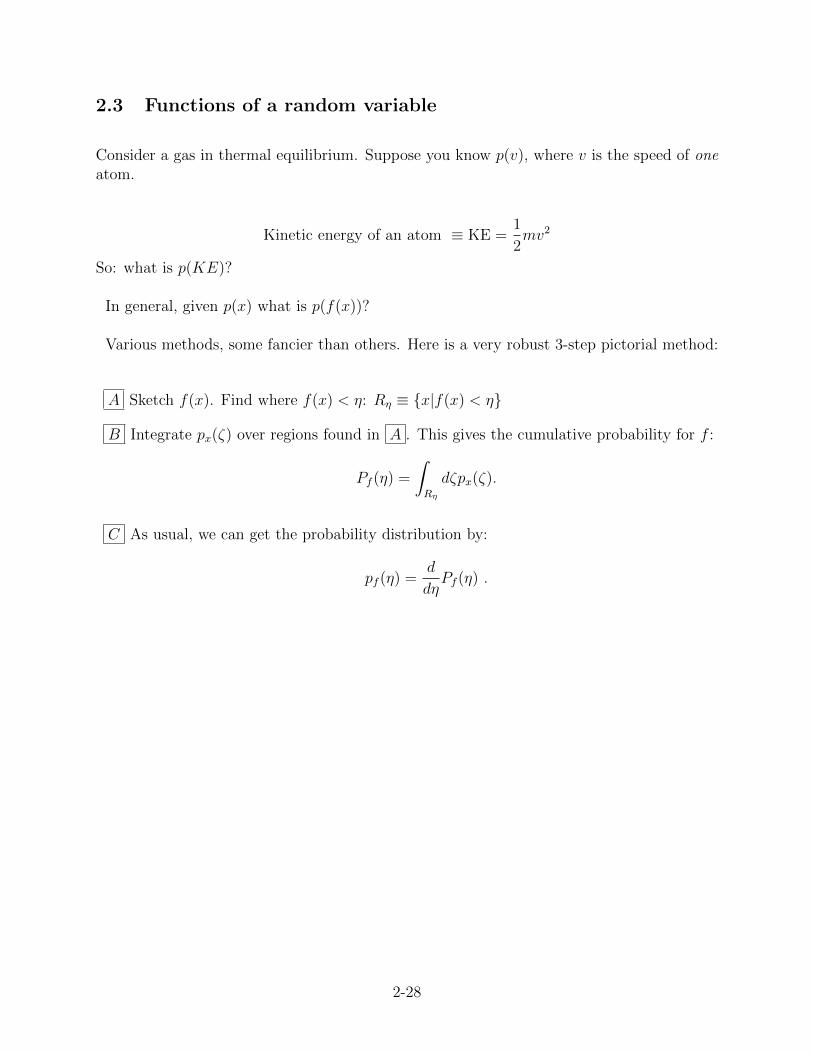
2.3 Functions of a random variable

Consider a gas in thermal equilibrium. Suppose you know p(v), where v is the speed of oneatom.

Kinetic energy of an atom ≡ KE =1

2mv2

So: what is p(KE)?

In general, given p(x) what is p(f(x))?

Various methods, some fancier than others. Here is a very robust 3-step pictorial method:

A Sketch f(x). Find where f(x) < η: Rη ≡ {x|f(x) < η}

B Integrate px(ζ) over regions found in A . This gives the cumulative probability for f :

Pf (η) =

∫Rη

dζpx(ζ).

C As usual, we can get the probability distribution by:

pf (η) =d

dηPf (η) .

2-28

Example 1: Kinetic energy of an ideal gas.

We’ll see much later in the course that a molecule or atom in an ideal gas has a velocitydistribution of the form:

p( vx︸︷︷︸x−component of velocity

) =1√

2πσ2exp[− v2

x

2σ2] with σ =

√kT/m

(same for vy, vz. let’s ignore those for now)

Define KEx ≡ 12mv2

x. What’s the resulting p(KEx)?

A Rη = [−√

2η/m,√

2η/m].

B

PKEx(η) =

√2η/m∫

−√

2η/m

pvx(ζ)dζ

And: DON’T DO THE INTEGRAL!

C

pKEx(η) =d

dηPKEx =

1√2mη

pvx(√

2η/m)− (− 1√2mη

)pvx(√

2η/m)

2-29

p(KEx) =

1√

πmσ2KExexp[−KEx

mσ2 ], for KEx > 0

0 for KEx < 0

Not gaussian at all! Completely different shape fromp(vx).

Whence the divergence? As v → 0, dvdKEx

→ ∞. =⇒Pileup at v = 0.

ΚΕ

v

dv

dKE

[End of Lecture 5.]

Note that pf (η) is in general a completely different function from px(ζ). This is the purposeof the pedantic notation with the subscripts and the dummy variables. A more concisestatement of their relationship is

pf (η) =

∫ ∞−∞

dζpx(ζ)δ(η − f(ζ)).

Unpacking this neat formula is what’s accomplished by the 3-step graphical method. Let’swork another example with that method.

2-30

Example 2: Hockey puck distribution again.

p(x, y) =

1π, for x2 + y2 ≤ 1

0, for x2 + y2 > 1

.

This the same as the paint droplet problem on pset 2.

Find p(r, θ).

A : pick some r, θ. Sketch the regionRr,θ ≡ {(r′, θ′)|r′ < r, θ′ < θ}.

B :

P (r, θ) =

∫Rr,θ

dxdyp(x, y) =

∫ r

0r′dr

∫ θ0dθ′ 1

π= 1

ππr2 θ

2πfor r < 1

θ2π

for r > 1.

It’s just the fraction of the area of the disc taken up by Rr,θ.

C :

p(r, θ) = ∂r∂θP (r, θ) =

{rπ

r < 1

0 r > 1

Check against pset 2:

p(r) =

∫ 2π

0

p(r, θ)dθ =

{2r r < 1

0 r > 1

p(θ) =

∫ 2π

0

p(r, θ)dr =r2

2π|10 =

1

2π

Note: p(r, θ) = p(r)p(θ). With this joint distribution r, θ are SI, although x, y are not.

2-31

2.4 Sums of statistically-independent random variables

Variables describing the macrostate of a gas in the thermodynamic limit = sums of 1023

variables describing the individual particles.

Energy ideal gas: E =∑1023

i=1 KEi

Claim: “all of thermodynamics is about sums of SI RVs”. (a more accurate claim: we canget all of the effects of thermodynamics from sums of SI RVs.)

Consider N SI RVs xi, i = 1..N . Let SN ≡∑N

i=1 xi. (Note: pxi(ζ) need not be independentof i.)

〈SN〉 =

∫dx1...dxN SN︸︷︷︸

=x1+x2+...+xN

p(x1, x2...xN)

=N∑i=1

∫dxixip(xi) =

N∑i=1

〈xi〉 (5)

All the other integrals are just squashing in N − 1 dimensions.Mean of sum is sum of means (whether or not RVs are SI).

Var(SN) = 〈(SN − 〈SN〉)2〉

= 〈(x1 − 〈x1〉+ x2 − 〈x2〉+ ...+ xN − 〈xN〉)2〉

=∑ij

〈(xi − 〈xi〉) (xj − 〈xj〉)〉

=∑ij

(〈xixj〉 − 〈xi〉〈xj〉)

=∑i 6=j

0︸︷︷︸by SI

+∑i=j

(〈x2

i 〉 − 〈xi〉2)

Var(SN) =N∑i=1

Var(xi) (6)

More on that crucial step:

〈xixj〉 =

∫dx1..dxN p(x1...xN)xixj

SI=

∫..p(xi)...p(xj)...xixj

2-32

= (

∫dxip(xi)xi)(

∫dxjp(xj)xj)

= 〈xi〉〈xj〉 (7)

Correlation functions of SI RVs factorize.

SO:Var(sum) = sum(Variances) if RVs are SI

Crucial note: where correlations, this statement is not true. Suppose given distributionsfor two variables (results of squashing): p(x1), p(x2).

example 1: Suppose perfect correlation: p(x1, x2) = δ(x1 − x2)p(x1) .In every copy of the ensemble, x1 = x2.Claim: then Var(sum) = 4 Var(x1).

example 2: Suppose perfect anticorrelation: p(x1, x2) ∝ δ(x1 + x2).The sum is always zero! So Var(x1 + x2) = 0.

“iid” RVs

Consider n SI RVs, x1..xn. If all p(xi) are the same, and the xi are SI, these are (naturally)called “independent and identically distributed” (“iid”). Let 〈xi〉 ≡ 〈x〉, Var(xi) ≡ σ2. Then

〈Sn〉 = n〈x〉, Var(Sn) = nσ2

As n→∞,〈Sn〉 ∝ n, Var(Sn) ∝ n, stdev(Sn) ∝

√n .

=⇒ stdev(Sn)

〈Sn〉∝ 1√

n. The distribution gets narrower as n→∞.

Notes:

• This statement is still true if the p(xi) are different, as long as no subset dominatesthe mean. (i.e. it’s not like: 1000 vars, 999 with 〈xi〉 = 1 and one with x? = 1052. )

• We assumed means and variances are all (nonzero and) finite.

• This applies for both continuous and discrete RVs.

• This is the basis of statements like: “The statistical error of the opinion poll was x”.That means that x2 people were polled.

2-33

Towards the central limit theorem.

So far we know 〈Sn〉,VarSn. What can we say about the shape of p(Sn)?

Answer first for two vars x, y. s ≡ x + y. Given px,y(ζ, η), what’s p(s)? One way to do itis:

p(s) =

∫dζdη px,y(ζ, η)δ(s− (ζ + η)).

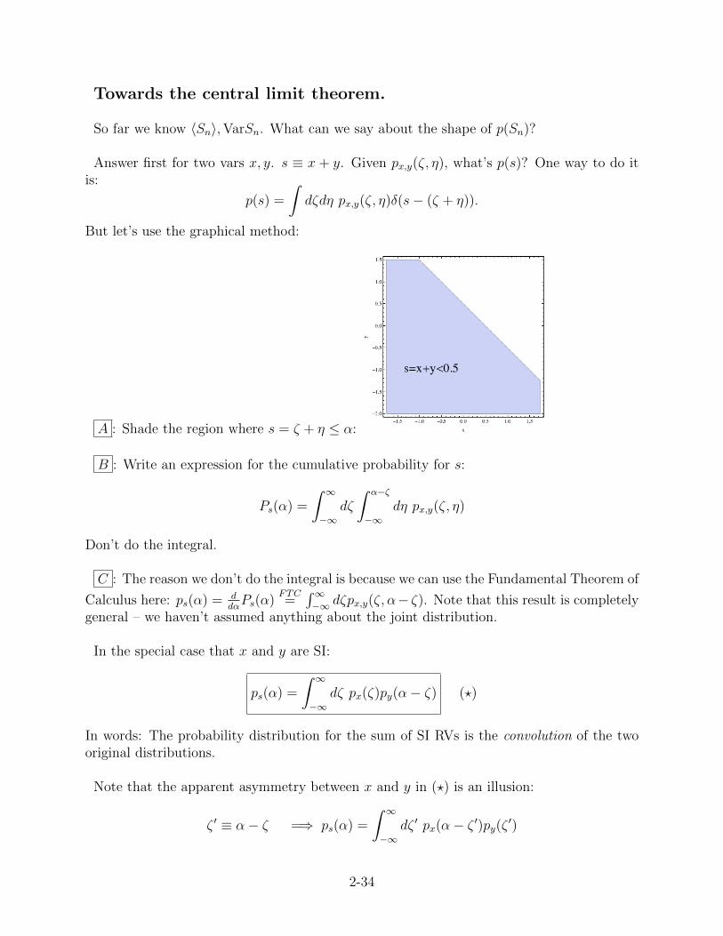
But let’s use the graphical method:

A : Shade the region where s = ζ + η ≤ α:

B : Write an expression for the cumulative probability for s:

Ps(α) =

∫ ∞−∞

dζ

∫ α−ζ

−∞dη px,y(ζ, η)

Don’t do the integral.

C : The reason we don’t do the integral is because we can use the Fundamental Theorem of

Calculus here: ps(α) = ddαPs(α)

FTC=∫∞−∞ dζpx,y(ζ, α− ζ). Note that this result is completely

general – we haven’t assumed anything about the joint distribution.

In the special case that x and y are SI:

ps(α) =

∫ ∞−∞

dζ px(ζ)py(α− ζ) (?)

In words: The probability distribution for the sum of SI RVs is the convolution of the twooriginal distributions.

Note that the apparent asymmetry between x and y in (?) is an illusion:

ζ ′ ≡ α− ζ =⇒ ps(α) =

∫ ∞−∞

dζ ′ px(α− ζ ′)py(ζ ′)

2-34

[Mathy aside on convolutions: given two functions f(x), g(x), their convolution is definedto be

(f ⊗ g)(x) ≡∫ ∞−∞

dzf(z)g(x− z).

A few useful properties of this definition that you can show for your own entertainment:

f ⊗ g = g ⊗ f

f ⊗ (g + h) = f ⊗ g + f ⊗ h

f ⊗ (g ⊗ h) = (f ⊗ g)⊗ h

Fourier transform of convolution is multiplication. ]

2-35

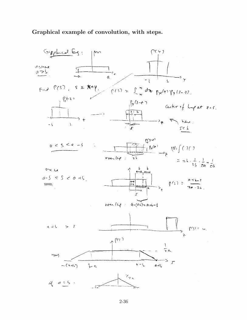
Graphical example of convolution, with steps.

2-36

Lessons

Lesson 1: convolution changes the shape.Lesson 2: convolution makes the result more gaussian.If you don’t believe it, do it again:

See Greytak for more details on p(sum of 4 RVs).

Three famous exceptions to lessons:

1) Gaussians: Consider two gaussian RVs:

px(x) =1√

2πσ2x

e− (x−a)2

2σ2x , py(y) =1√

2πσ2y

e− (y−b)2

2σ2y .

Claim [algebra, Greytak]: p(s = x+ y) = (px ⊗ py)(s) is gaussian. By our previous analysisof SI RVs, we know its 〈s〉,Var(s). So if it’s gaussian:

p(s) =1√

2π (σ2x + σ2

y)︸ ︷︷ ︸Vars add

exp[−(s− (a+ b))2

2(σ2x + σ2

y)]

2-37

2) Poisson: Claim [algebra, Greytak]: Sum of two SI Poisson RVs is also Poisson distributed.with mean = sum of means = variance. (Recall that a Poisson distribution is fully specifiedby the mean.)

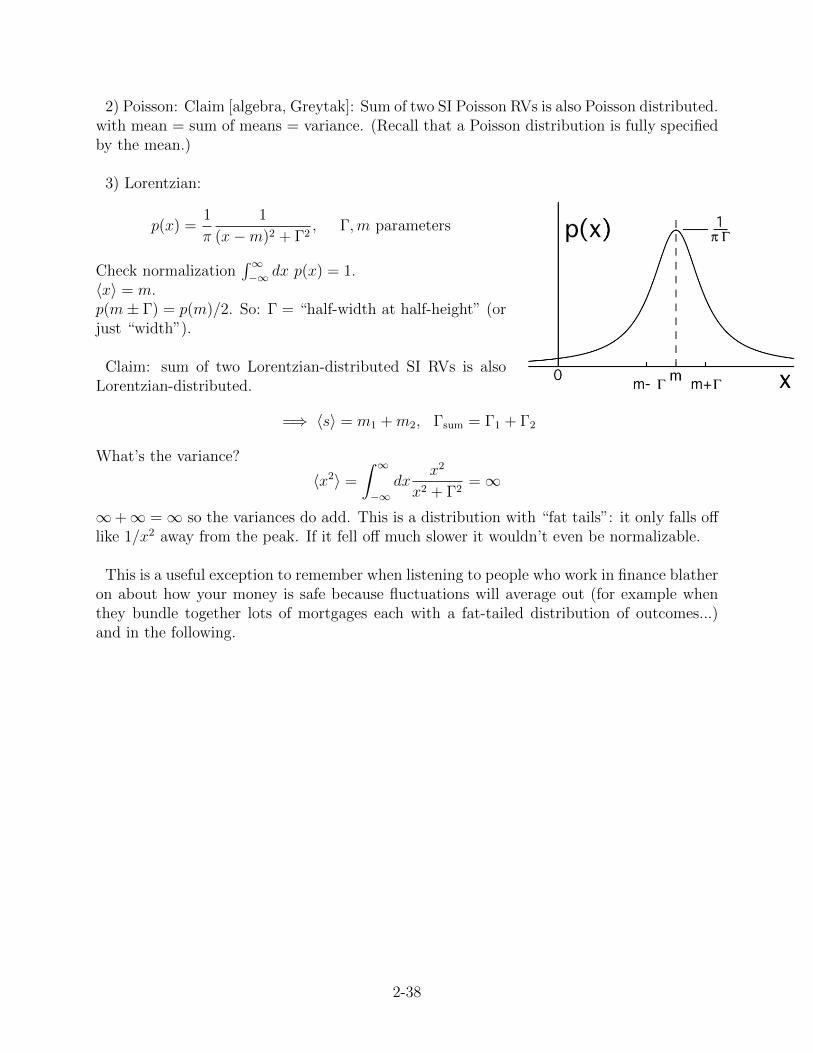
3) Lorentzian:

p(x) =1

π

1

(x−m)2 + Γ2, Γ,m parameters

Check normalization∫∞−∞ dx p(x) = 1.

〈x〉 = m.p(m± Γ) = p(m)/2. So: Γ = “half-width at half-height” (orjust “width”).

Claim: sum of two Lorentzian-distributed SI RVs is alsoLorentzian-distributed.

=⇒ 〈s〉 = m1 +m2, Γsum = Γ1 + Γ2

What’s the variance?

〈x2〉 =

∫ ∞−∞

dxx2

x2 + Γ2=∞

∞+∞ =∞ so the variances do add. This is a distribution with “fat tails”: it only falls offlike 1/x2 away from the peak. If it fell off much slower it wouldn’t even be normalizable.

This is a useful exception to remember when listening to people who work in finance blatheron about how your money is safe because fluctuations will average out (for example whenthey bundle together lots of mortgages each with a fat-tailed distribution of outcomes...)and in the following.

2-38

Central Limit Theorem (CLT)

Let sn = sum of n SI RVs, which are identically distributed (so: iid) (?)with mean 〈x〉 and variance σ2

x (which must be finite (??)).For large n (? ? ?),p(sn) can often be well-represented by (? ? ??)a gaussian, with mean n〈x〉, and variance nσ2

x.

i.e. p(sn) ≈︸︷︷︸can be well-rep. by

1√2πnσ2

x

exp[−(sn − n〈x〉)2

2nσ2x

]

Fine print

(?): The theorem also works if not identical, as long as no subset dominates s.

(??): Think of Lorentzians. Convolving many distributions with fat tails gives anotherdistribution with fat tails, i.e. the fluctuations about the mean are still large.

(? ? ?): The mathematicians among us would like us to say how large n has to be in orderto achieve a given quality of approximation by a guassian. This is not our problem,because n ∼ 1023 gives an approximation which is good enough for anyone.

(????): The reason for vagueness here is an innocent one; it’s so that we can incorporate thepossibility of discrete variables. For example, flip a coin 1000 times. The probabilitydistribution for the total number of heads looks like a gaussian if you squint just alittle bit: the envelope of the histogram is gaussian. This is what we mean by “can bewell-represented by”. (More on this next.)

This is why we focus on gaussians.

An example: consider a sum of many independent Poisson-distributed variables. I alreadyclaimed that convolutions of Poissons is again Poisson. How is this consistent with theCLT which says that the distribution for the sum of Poisson-distributed SI RVs should begaussian? When we sum more such (positive) RVs the mean also grows. The CLT meansthat (the envelope for) the Poisson distribution with large mean must be gaussian. (Lookback at Poisson with 〈n〉 = rL = 25 and you’ll see this is true.)

We will illustrate the origin of the CLT with an example. We’ll prove (next) that it worksfor many binomially-distributed SIRVs.

[End of Lecture 6.]

2-39

Flipping a coin (pset 1) A discrete example.

N = 1000 flips pN(n) ≡ Prob(n heads). 〈n〉 = 500 = N/2.

pset 1: pN(n) =1

2N︸︷︷︸total # of possible outcomes

× N !

n!(N − n)!︸ ︷︷ ︸# of ways to get n heads

Claim: This (binomial distribution) becomes a gaussian in the appropriate circumstances.More precisely, it becomes a comb of δ-functions with a Gaussian envelope.

Let n = N2

+ ε. ε ≡ deviation from mean. Since the distribution only has support whenε� N/2, we will make this approximation everywhere below.

p

(N

2+ ε

)=

1

2NN !(

N2

+ ε)!(N2− ε)!

The log of a function is always more slowly-varying than the function itself; this means thatit is better-approximated by its Taylor series; for this reason let’s take the log of both sides.

Use Stirling’s approximation (lnN !N�1≈ N lnN −N , valid for N � 1):

ln p

(N

2+ ε

)N�1≈ N ln 1/2 +N lnN −N

−(N2

+ ε)

ln(N2

+ ε)

+N/2 + ε

−(N2− ε)

ln(N2− ε)

+N/2− ε

2-40

Now expand about the mean (which is also the maximum) of the distribution ε = 0, using

ln(N/2± ε) ≈ lnN/2± 2ε/N − (2ε/N)2/2 +O(εN

)31

ln p

(N

2+ ε

)ε�N/2,N�1≈ N lnN/2

−(N/2 + ε)

(lnN/2 + 2ε/N − 1

2(2ε/N)2

)−(N/2− ε)

(lnN/2− 2ε/N − 1

2(2ε/N)2

)(8)

Collect terms by powers of ε:

ln p

(N

2+ ε

)ε�N/2,N�1≈ ε0

(N lnN/2− N

2lnN/2− N

2lnN/2

)+ ε1

(− lnN/2 + lnN/2 +

2ε

N

N

2− 2ε

N

N

2

)+ ε2

(− 4

N+

1

2

(2

N

)2N

2+

1

2

(2

N

)2N

2

)+ ε3

(...

1

N2

)

Therefore:

ln p

(N

2+ ε

)≈ −2ε2

N

(1 +O

( εN

)).

Comments: First, the reason that the order-ε terms cancel is that we are expanding aroundthe maximum of the distribution. The statement that it is the maximum means that thederivative vanishes there – that derivative is exactly the linear term in the Taylor expansion– and that the second derivative is negative there; this is an important sign. Second, thenontrivial statement of the Central Limit Theorem here is not just that we can Taylorexpand the log of the distribution about the maximum. The nontrivial statement is thatthe coefficients of terms of higher order than ε2 in that Taylor expansion become small asN →∞. It is crucial here that the terms we are neglecting go like ε3

N2 .

Therefore: the probability distribution is approximately Gaussian:

p

(N

2+ ε

)≈ exp

(− ε2

N/2

).

These expressions are valid for ε small compared to the mean, but indeed the mean is

1(by O (x)3I mean “terms of order x3 which we are ignoring”)

2-41

N/2� 1.

p (n) ≈ exp

(−(n−N/2)2

N/2

)= N︸︷︷︸

fixed by normalization

exp

−(n− 〈n〉)2

2 σ2N︸︷︷︸

VarN (n)

It’s a gaussian with mean N/2 and variance VarN(n) = σ2

N = N/4.

This is consistent with the CLT quoted above. For one coin flip, 〈n〉 = 1/2, σ21 = Var(n) =

1/4.

The variance of the distribution of n after N flips is σ2n = Nσ2

1 = N/4 (Variance adds forIID RVs).

On pset 4 you’ll look at where the half-maximum occurs:

1

2= e−

(n−N/2)2N/2

ln 1/2 = −(n−N/2)2

N/2

n−N/2 =√N/2 ln 2 =

√log 2/2

√N =

√0.3466N.

and compare with your approximate treatment on pset 1 which gave√

0.333N .

2-42

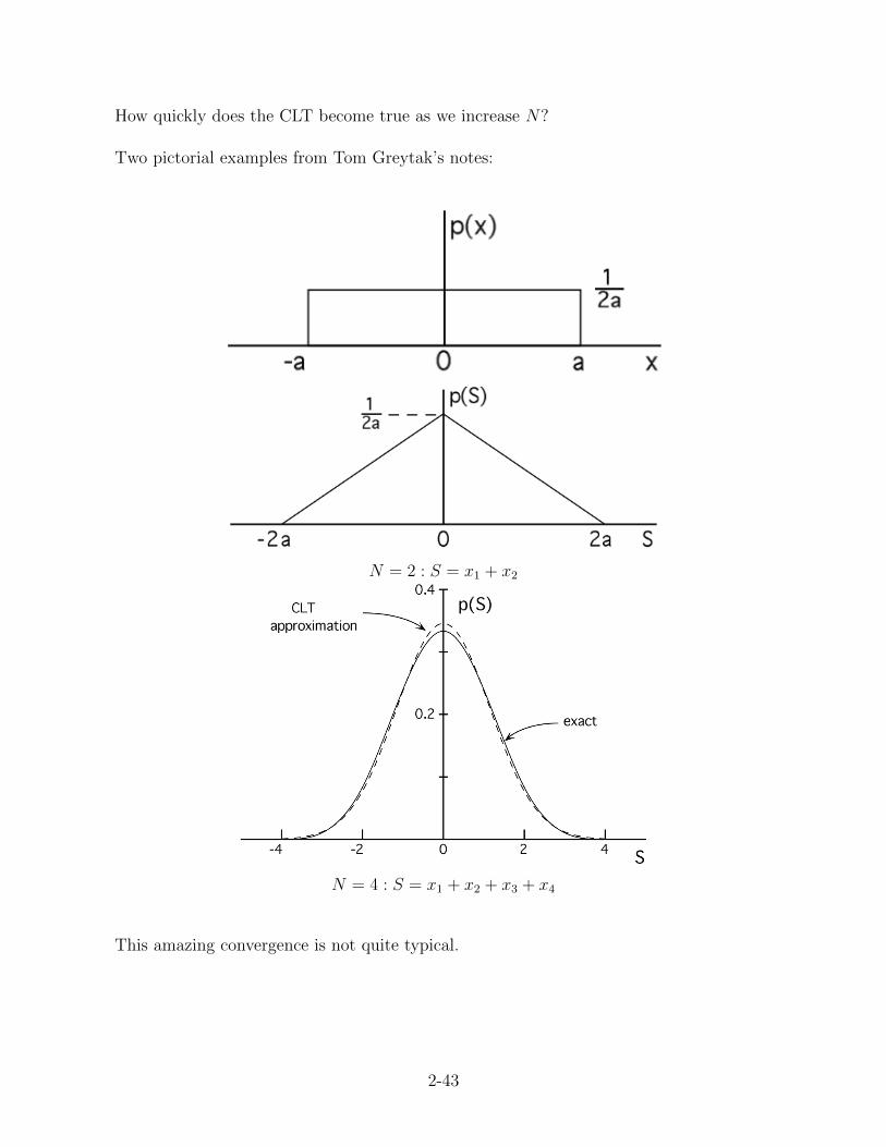
How quickly does the CLT become true as we increase N?

Two pictorial examples from Tom Greytak’s notes:

N = 2 : S = x1 + x2

N = 4 : S = x1 + x2 + x3 + x4

This amazing convergence is not quite typical.

2-43

Some more convolutions, in Tom Greytak’s notes. Consider the one-variable distribution:

p(x) =

1ae−x/a, for x ≥ 0

0, for x < 0

Let S =∑n

i=1 xi where each xi is governed by the density p(x). For simplicity, set a = 1.

Claim [do convolutions]:

pn(S) =

Sn−1e−S

(n−1)!, for S ≥ 0

0, for S < 0

2-44

An example from physics: energy of molecules in ideal gas

Previously we considered the distribution for ‘kineticenergy of one atom due to motion in the x direction’:

p(KEx) =1√

πmσ2KEx

e−KExmσ2 σ2 = kT/m

We’ll derive this in a few weeks. For now, it’s our startingpoint. On pset 4 you’ll play with this distribution and inparticular will show that

〈KEx〉 =1

2kT Var(KEx) =

1

2(kT )2 .

Consider N such atoms in a (3-dimensional) room, each atom with this distribution for itsKEx,KEy,KEz. We ignore interactions between the atoms.

Energy of N atoms in 3d: E = (KEx + KEy + KEz)atom 1+(KEx + KEy + KEz)atom 2 +...

Assume: each of these variables is statistically independent from all the others. (That is,(KEx)atom 1 and (KEy)atom 1 are SI AND (KEx)atom 1 and (KEx)atom 2 are SI and so on....)Then we have for sums of RVs that the means add:

〈E〉 =∑〈each KE〉 = 3N · 1

2kT =

3

2NkT

And for sums of SI RVs that the variances add as well:

Var(E) =3

2N(kT )2.

Then the CLT tells us what the whole distribution for E is:

p(E) =1√

2π 32N(kT )2

exp

[−

(E − 32NkT )2

2 · 32N(kT )2

]

This is with N = 105 (in units where 32kT = 1).

2-45

Very small fluctuations about the mean!

width

mean∼√

Var

mean=kT√

32N

32N

∼ 1√N∼ 10−25/2.

Our discussion of the CLT here assumed that the vars we were summing were SI. The CLTactually still applies, as long as correlations are small enough.

Atoms in a real fluid are not SI. An occasion where correlations lead to important fluctu-ations is at a critical point. See 8.08 or 8.333.

2-46

2.5 Epilog: an alternate derivation of the Poisson distribution

Here is a discussion of an origin of the Poisson distribution complementary to the carefulone in Prof. Greytak’s notes.

2.5.1 Random walk in one dimension

A drunk person is trying to get home from a bar at x = 0, and makes a series of stepsof length L down the (one-dimensional) street. Unfortunately, the direction of each step israndom, and uncorrelated with the previous steps: with probability p he goes to the rightand with probability q = 1 − p he goes to the left. Let’s ask: after N steps, what’s hisprobability P(m) of being at x = mL?

Note that we’ve assumed all his steps are the same size, which has the effect of makingspace discrete. Let’s restrict ourselves to the case where he moves in one dimension. Thisalready has many physical applications, some of which we’ll mention later.

What’s the probability that he gets |m| > N steps away? With N steps, the farthest awayhe can get is |m| = N , so for |m| > N , P (m) = 0.

Consider the probability of a particular, ordered, sequence of N steps, xi = L or R:

P (x1, x2...xN) = P (x1)P (x2) · · ·P (xN) = pnRqnL .

In the second step here we used the fact that the steps are statistically independent, so thejoint probability factorizes. nR is the number of steps to the right, i.e. the number of the xiwhich equal R. Since the total number of steps is N , nL + nR = N , the net displacement(in units of the step length L) is

m = nR − nL = 2NR −N.

Note that m = N mod two.

In asking about the drunk’s probability for reaching some location, we don’t care aboutthe order of the steps. There are many more ways to end up near the starting point thanclose by. For example, with N = 3, the possibilities are

LLL m = −3

RLL,LRL,LLR m = −1

RRL,RLR,LRR m = 1

RRR m = 3

2-47

What’s the number of sequences for a given nL, nR? The sequence is determined if we saywhich of the steps is a R, so we have to choose nR identical objects out of N . The numberof ways to do this is (

NnR

)=

N !

nR!nL!=

(NnL

).

A way to think about this formula for the number of ways to arrange N = nR + nL ofwhich nR are indistinguishably one type and nL are indistinguishably another type, is: N !is the total number of orderings if all the objects can be distinguished. Redistributing thenR R-steps amongst themselves doesn’t change the pattern (there are nR! such orderings),so we must divide by this overcounting. Similarly redistributing the nL L-steps amongstthemselves doesn’t change the pattern (there are nL! such orderings).

So

P (nL, nR) =N !

nR!nL!pnRqnL .

Note that the binomial formula is

(p+ q)N =N∑n=0

N !

n!(N − n)!pnqN−n.

Since we have p+ q = 1, this tells us that our probability distribution is normalized:

N∑nR=0

N !

nR!(N − nR)!pnRqN−nR = 1N = 1.

The probability for net displacement m is

P (m) =N !(

N+m2

)!(N−m

2

)!pN+m

2 qN−m

2

for N ±m even, and zero otherwise.

2.5.2 From binomial to Poisson

We have shown that the probability that an event with probability p occurs n times in N(independent) trials is

WN(n) =N !

n!(N − n)!pn(1− p)N−n ;

this is called the binomial distribution. 1 − p here is the probability that anything elsehappens. So the analog of ”step to the right” could be ”a particular song is played on youripod in shuffle mode” and the analog of ”step to the left” is ”any other song comes on”.

2-48

For example, suppose you have 2000 songs on your ipod and you listen on shuffle by song;then the probability of hearing any one song is p = 1

2000. Q: If you listen to N = 1000 songs

on shuffle, what’s the probability that you hear a particular song n times?

The binomial distribution applies. But there are some simplifications we can make. First,p itself is a small number, and N is large. Second, the probability will obviously be verysmall for n ∼ N , so let’s consider the limit n � N . In this case, we can apply Sterling’sformula to the factorials:

WN(n) ≈ 1

n!

NN

(N − n)N−npn(1− p)N−n

We can use N − n ∼ N except when there is a cancellation of order-N terms:

WN(n) ≈ 1

n!

NN

(N)N−npn(1− p)N−n =

1

n!Nnpn(1− p)N−n

Now we can taylor expand in small p, using ln(1− x) ≈ −x+ x2/2− x3/3 + ...

WN(n) ≈ 1

n!(Np)ne(N−n) ln(1−p) ≈ 1

n!(Np)ne−Np.

This is called the Poisson distribution,

Poissonµ(n) =1

n!µne−µ.

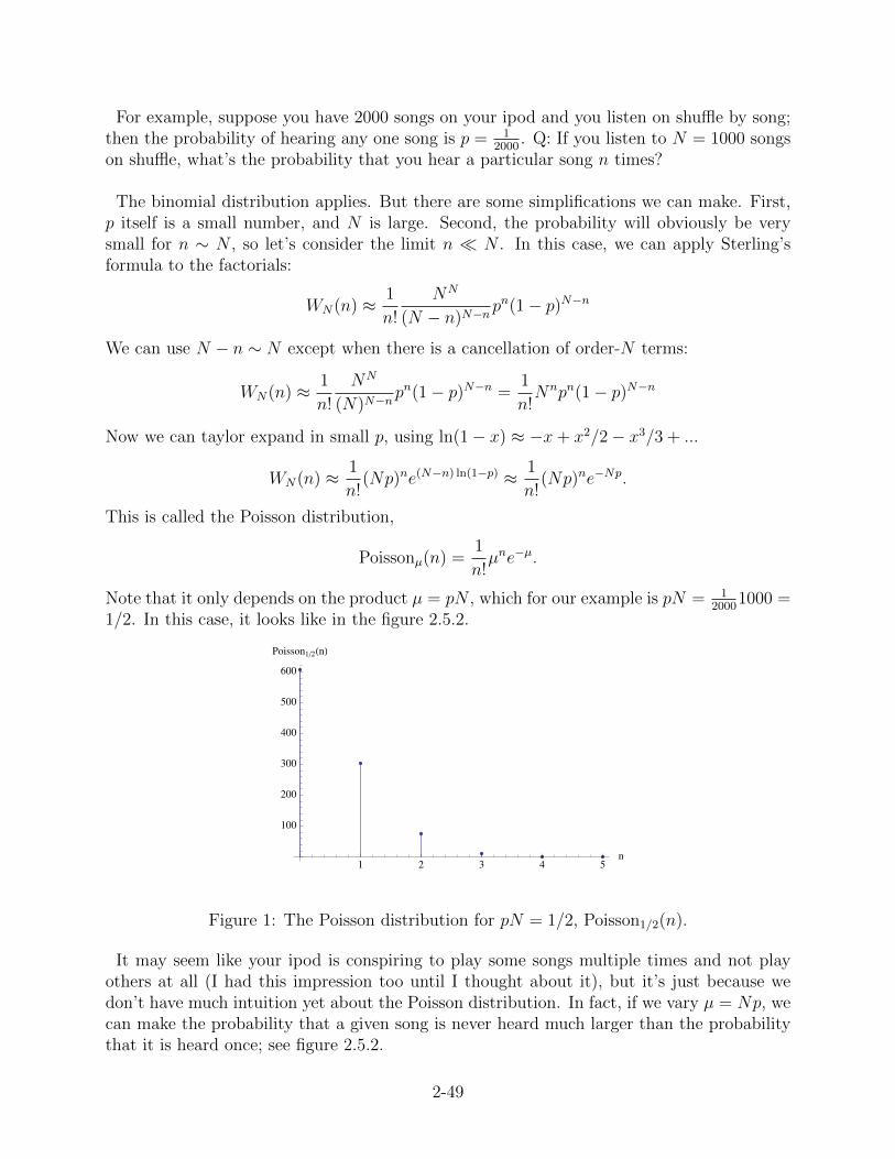
Note that it only depends on the product µ = pN , which for our example is pN = 12000

1000 =1/2. In this case, it looks like in the figure 2.5.2.

1 2 3 4 5n

100

200

300

400

500

600

Poisson1�2HnL

Figure 1: The Poisson distribution for pN = 1/2, Poisson1/2(n).

It may seem like your ipod is conspiring to play some songs multiple times and not playothers at all (I had this impression too until I thought about it), but it’s just because wedon’t have much intuition yet about the Poisson distribution. In fact, if we vary µ = Np, wecan make the probability that a given song is never heard much larger than the probabilitythat it is heard once; see figure 2.5.2.

2-49

1 2 3 4Μ

0.5

1.0

1.5

Poisson H0L

Poisson H1L

Figure 2: The ratio of the poisson distribution at n = 0 to n = 1 as we vary the parameterµ. (Note that this figure is not a probability distribution.)

2-50