82286 16 solution - cengage 35,000 rework 70,000 correcting imperfections 6,250 rework due to vendor...

SOLUTIONS TO EVEN-NUMBERED PROBLEMS

CHAPTER 8

2. The general conclusion that can be reached for Imagimatrix from inspecting thedata is that costs for internal and external failure are larger than they should be(totaling 47% of quality costs). Improvements that have been made to date haveprobably involved increasing prevention and appraisal costs that now stand atmore than 50% of the total quality costs. Since appraisal costs are a large per-centage of costs, and internal failures are a larger percentage than external fail-ures, it is likely that quality is being “inspected in,” and many defective itemsare being taken out and reworked after being caught by inspection. Moremoney and time needs to be invested in prevention, which will reduce defectsand costs in other areas in a fairly short time.

4. An Excel chart can be constructed to show details on Product B sales and costof quality presented in the problem, along with information on the percentageof total quality cost attributable to each cost category (external, internal,appraisal, and prevention). This problem contains time-phased data, unlikeproblem 1. Thus it is possible to calculate an index base and quarterly indicesfor the various cost categories. The data show that the external and internal fail-ure indices, as well as the appraisal index, are declining, while the preventionindex is increasing. The overall quality cost index as a percent of sales is alsodeclining. This is an ideal situation in which managers of the B product line arecontinuing to put more emphasis on prevention and attempting to reduce costsin other categories.

6. The data can be rearranged as follows:

Type of Cost Cost Category $ Cost % of COQ

Inspection and retest Appraisal 340,000 38.9Scrap Int. failure 330,000 37.8Customer returns Ext. failure 90,000 10.3Repair Int. failure 80,000 9.2Quality equipment design Prevention 25,000 2.9Supplier quality surveys Prevention 8,000 0.9

$ Costs % of COQ

Internal failure 410,000 47.0External failure 90,000 10.3Appraisal 340,000 38.9Prevention 33,000 3.8

873,000

Although scrap is part of the process, Smith Company needs to minimize theamount of scrap produced, just as if it were making a product. The total cost ofquality is $873,000. Although the categories are not completely clear, theassumed categories are listed in the revised table above. Internal failure (scrapand repair) total 47% of quality costs, and external failure in the form of cus-tomer returns adds another 10.3%. Only 3.8 % of total costs are being applied toprevention. Apparently, based on high internal failure and appraisal costs, thisorganization is attempting to screen out bad product and scrap or repair it.

Solutions to Even-Numbered Problems S-1

82286_16_Solution.qxd 12/12/06 4:54 PM Page S-1

Also, on this batch, they didn’t accomplish their goal of 60% of book value goalbecause (1,700,000 – 873,000)/1,700,000 = 48.65 %.

8. Miami Valley Aircraft Service Company’s data show rapidly decreasing totalquality costs (except for a slight rise in the 4th quarter), possibly due to a con-certed quality effort. The decrease in both internal and external quality costs, asa percentage of total quality and labor costs, while the prevention costs per-centage is rising, is good. The only recommendation would be to increase pre-vention costs even more rapidly, while holding the line on appraisal costsHowever, the caution is that doing so may increase total quality costs in theshort run, as may have happened in the 2nd quarter.

Percentages Quarterly Quality/Labor Costs

1 Qtr. 2 Qtr. 3 Qtr. 4 Qtr.

External failure 5.13 4.74 4.52 3.82Internal failure 17.95 17.11 14.29 11.58Appraisal 4.62 6.32 5.48 4.53Prevention 2.05 2.63 2.62 4.21Total Quality/Labor Cost 29.74 30.79 26.90 24.13

10. Spreadsheet data and the Pareto chart for Repack Solutions, Inc. show that thecompany is spending too much on appraisal and internal failure cost and toolittle on prevention. Checking boxes, machine downtime, and packaging wasteneed immediate improvement to have the greatest impact on quality costsbecause they constitute almost 82% of quality costs. However, it should be donewith caution because “checking boxes” represents appraisal costs designed toscreen out poor quality and prevent it from reaching the customer.

Repack Solutions, Inc. Quality Cost & Percentages

Quality Cost

Percent Cumulative % Cost ($) Category

Checking boxes 48.80 48.80 710,000 AppraisalMach. downtime 27.84 76.63 405,000 Int. Fail.Pkg. waste 5.15 81.79 75,000 Int. Fail.Income. insp. 4.12 85.91 60,000 AppraisalOther waste 3.78 89.69 55,000 Int. Fail.Cust. complaints 2.75 92.44 40,000 Ext. Fail.Error corrn. 2.75 95.19 40,000 Int. Fail.Qual. train. assoc. 2.06 97.25 30,000 Prevent.Improv. proj. 1.37 98.63 20,000 Prevent.Typo corrn. 0.69 99.31 10,000 Int. Fail.Quality planning 0.69 100.00 10,000 Prevent.Total 1,455,000

Note that costs could also be classified by aggregating them into the four cate-gories of internal and external failure, prevention, and appraisal costs, insteadof the categories listed in the table.

12. For HiTeck Tool Company, the largest costs are internal failure (56.6%) andappraisal (27.1%). More must be done in quality training, a component of pre-vention (currently 7.8%), if failure, appraisal, and overall quality costs are to becontrolled. External failure costs are 8.6% of quality costs, so screening methodsare working fairly well. Note that the proportions are fractions of the total qualitycosts of $247,450.

S-2 Solutions to Even-Numbered Problems


Quality Cost Categories

Cost Elements Costs ($) Subtotal Proportion

APPRAISALIncoming test & inspection 7,500Inspection 25,000Test 5,000Laboratory testing 1,250Design of Q.A. equipment 1,250Material testing & insp. 1,250Insp. equipt. & calibration 2,500Formal complaints to vendors 10,000Setup for test & inspection 10,750Laboratory services 2,500

$67,000 0.271

PREVENTIONQuality training 0Quality audits 2,500Maintenance of tools and dies 9,200Quality control admin. 5,000Writing proced. & instr. 2,500

$19,200 0.078INTERNAL FAILURE COSTSScrap 35,000Rework 70,000Correcting imperfections 6,250Rework due to vendor faults 17,500Problem solving—prod. engrs. 11,250

$140,000 0.566EXTERNAL FAILURE COSTSAdjustment cost of complaints 21,250

$21,250 0.086

Total costs $247,450

14. The data for Beechcom Software Corporation show that the three categories ofrejected disks (loaded), returns, and system downtime account for 74.64 percentof the defects. These appear to be completely under the control of the firm, sosteps should be taken to analyze root causes for these problem areas in order tocorrect them as quickly as possible.

Beechcom Software Corporation Quality Costs and Percentages

Percent Cumulative % Cost ($)

Rej. disks (load.) 39.34 39.34 360,000Returns 20.22 59.56 185,000Sys. Downtime 15.08 74.64 138,000Rej. disks (blank) 9.73 84.37 89,000Trng./sys. improve. 7.32 91.69 67,000Rework costs 3.28 94.97 30,000Insp.—Out 3.06 98.03 28,000Insp.—In. 1.97 100.00 18,000

Total Costs 915,000



16. This is a very challenging problem, even for advanced students. Although youmay fit a linear regression equation to the set of data given in the problem, fit-ting a curvilinear model would provide a higher R-squared value. This requiresa more complex solution process. There is no “cut and dried” answer to whatlevel of additional quality improvement effort would be best, of course.

A number of “what if” questions and scenarios could be raised. Some ofthese might include the following:1. What if the sample of hotel guests was not representative of the general popu-

lation of guests?2. What if the site manager was simply interested in reducing, rather than

“eliminating,” dissatisfied customers? 3. What if her objective was to eliminate the competition, then go back to the

previous level of quality?4. What are the disadvantages of fitting a linear model to the data? (Note: In using

Excel 4.0 when this solution was developed, it appears that there is a “bug” inthe module that calculates the equation for the graph. Therefore, the “add-in”Excel model was used to get the equation and the R-squared value, as follows.)

Excelsior Inn—Return on Quality

Svc. Improvemt. Percent of Customers— Predicted

Effort—$ 000 Dissatisfied Y—Regression Line

0 0.200 0.107550 0.150 0.1046

150 0.100 0.0987260 0.076 0.0922290 0.067 0.0905300 0.059 0.0899450 0.052 0.0811600 0.045 0.0723750 0.040 0.0635900 0.035 0.0547

1050 0.031 0.04591200 0.027 0.03711350 0.024 0.02831500 0.021 0.01951650 0.017 0.01071800 0.014 0.00191950 0.010 −0.00702100 0.007 −0.0158

Partial Summary Output

Excel Regression Analysis

Regression Statistics

Multiple R 0.795781742R Square 0.633268581Adjusted R Square 0.610347868Standard Error 0.031875396Observations 18

Coefficients

Intercept 0.107507099X Variable 1 –5.87234E-05



Equation: y = 0.10751 − .0000587 xi

Assume that we use the calculated value of y = 0 (no dissatisfied customers).The model tells us that we will have:

0 = 0.10751 − 0.0000587 xi

So xi = 0.10751/0.0000587 = $1831.5 thousand

We can calculate the net present value, using standard present value tablefigures of:

Year PV Factor for 10% Cost Present Value ($000)

1 0.909 1831.5 1664.832 0.826 1831.5 1512.823 0.751 1831.5 1375.46

Total Net Present Value 4553.11

The return on quality of: ROQ = Annual profit increase/discounted presentvalue of investment

ROQ = (2.5 points − market share increase × $600)/4553.11 = 32.9%, which is avery healthy return on investment

CHAPTER 10

2. The defect rate is 65/1000 = 0.065. This is the same as: 0.065 × 1,000,000 = 65,000dpmo. From Table 10.1, we see that this is slightly better than 3 sigma with offcentering of 1.5 sigma.

4. We use 3/1054 to get the number of defects per unit (DPUs). However, there are2 opportunities per injection (wrong drug, wrong dosage) to make an error.They must be considered to calculate dpmo.

dpmo = (3/1054) × 1,000,000/2 = 1423.1, which is slightly less than 4.5 sigmawith off centering of 1.5 sigma.

6. To calculate the overall dpmo and sigma level, we have:

dpmo = (6/5000) × 1,000,000/5 = 240, which is approximately 5 sigma with off-centering of 1.5 sigma.

But for the one characteristic, we have:

dpmo = (2/5000) × 1,000,000 = 400, which is still good, but somewhat less than5 sigma with off centering of 1.5 sigma.

A Six Sigma project should be launched to determine root causes for the defectsfrom this one characteristic.

CHAPTER 11

2. The following results were obtained from the Staunton Steam Laundry Data



Column1

Mean 34.280Standard Error 3.241Median 25.500Mode 19.000Standard Deviation 32.412Sample Variance 1050.507Kurtosis 3.847Skewness 1.756Range 169.000Minimum 1.000Maximum 170.000Sum 3428.000Count 100.000Largest(1) 170.000Smallest(1) 1.000Confidence Level(95.0%) 6.431

The conclusion that can be reached from looking at the summary statistics andthe histogram is that these data are exponentially distributed, with descendingfrequencies. These data may show errors, by category, which are best repre-sented by a histogram.

4. Descriptive statistics for the Harrison Metalwork foundry are shown in thefollowing chart:

Descriptive Statistics

Mean 38.6320Standard Error 0.0444Median 38.6000Mode 38.4000Standard Deviation 0.4436Sample Variance 0.1967Range 2.6000Minimum 37.3000Maximum 39.9000Sum 3863.2000Count 100.0000


0

5

10

15

20

25

30

35

40

15 30 45 60 75 90 105 More

Measures

Fre

qu

en

cy

Frequency

Frequency Histogram


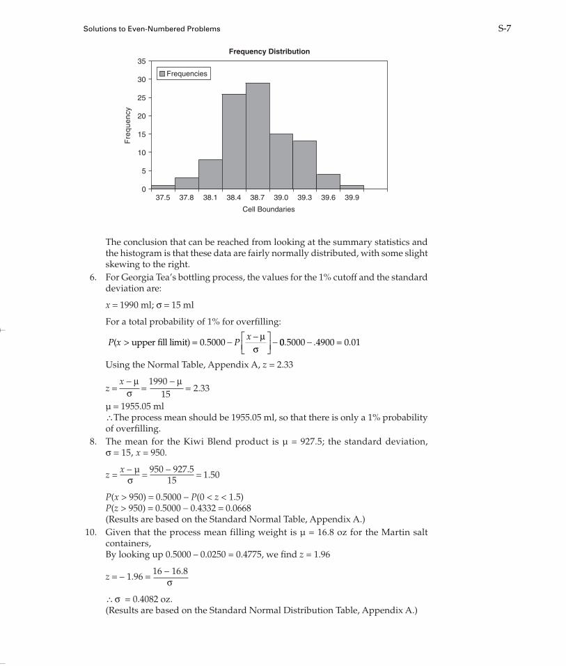
The conclusion that can be reached from looking at the summary statistics andthe histogram is that these data are fairly normally distributed, with some slightskewing to the right.

6. For Georgia Tea’s bottling process, the values for the 1% cutoff and the standarddeviation are:

x = 1990 ml; σ = 15 ml

For a total probability of 1% for overfilling:

Using the Normal Table, Appendix A, z = 2.33

z =x − µ

=1990 − µ

= 2.33σ 15µ = 1955.05 ml∴The process mean should be 1955.05 ml, so that there is only a 1% probabilityof overfilling.

8. The mean for the Kiwi Blend product is µ = 927.5; the standard deviation, σ = 15, x = 950.

z = x − µ = 950 − 927.5 = 1.50σ 15

P(x > 950) = 0.5000 − P(0 < z < 1.5)P(z > 950) = 0.5000 − 0.4332 = 0.0668(Results are based on the Standard Normal Table, Appendix A.)

10. Given that the process mean filling weight is µ = 16.8 oz for the Martin saltcontainers, By looking up 0.5000 – 0.0250 = 0.4775, we find z = 1.96

z = − 1.96 = 16 − 16.8σ

∴ σ = 0.4082 oz.(Results are based on the Standard Normal Distribution Table, Appendix A.)

P x Px

( > u fill limit)pper = − −

−0 5000.µ

σ00 5000 4900 0 01. . .− =


0

5

10

15

20

25

30

35

37.5 37.8 38.1 38.4 38.7 39.0 39.3 39.6 39.9

Cell Boundaries

Fre

qu

en

cy

Frequencies

Frequency Distribution


12. Adj. Cell

Midpoints Frequencies fx fx2

Cell 1 37.35 1 37.35 1395.02Cell 2 37.65 3 112.95 4252.57Cell 3 37.95 8 303.60 11521.62Cell 4 38.25 23 879.75 33650.44Cell 5 38.55 25 963.75 37152.56Cell 6 38.85 23 893.55 34714.42Cell 7 39.15 10 391.50 15327.23Cell 8 39.45 6 236.70 9337.82Cell 9 39.75 1 39.75 1580.06

3858.90 148931.73

b. Answer may be found in Problem 11-3.c. A normal probability plot shows that the data are approximately normally

distributed, with an R square value of 0.947.

a.fx

n3858.90

10038.589 (vs. 38.670 frox = ∑ = = mm the data in problem 11-3)

sfx

nfx= ∑

−− ∑2

1( )22 2

1148931 73

993858 9 100

99

0 4572

/ /nn −

= −

=

. ( . )

. ((versus 0.4556 from the spreadsheet data)


37

38

39

40

41

0 20 40 60 80 100

Sample Percentile

Y

Normal Probability Plot

14. Specification for answer time for the Tessler utility is:

H0: Mean response time: µ1 ≤ 0.10H1: Mean response time: µ1 > 0.10x−1 = 0.1023, s1 = 0.0183

and the t-test is:

Specification for service time is: H0: Mean service time: µ2 ≤ 0.50H1: Mean response time: µ2 > 0.50x−2 = 0.5290, s2 = 0.0902and the t-test is:

tx

s n2

0 50 0 529 0 500 0902 30

0 0290 0165

= − = − =. . ..

../

== =1 761 1 69929 05. , .,.t

t

xs n

10 10 0 1023 0 10

0 0183 300 00230 0

= − = − =. . ..

.

./ / 00330 697 1 69929 05= =. , .,.t


Because t29,.05 = 1.699, we cannot reject the null hypothesis for t1, but we canreject the hypothesis for t2. Therefore, there is no statistical evidence that themean response time exceeds 0.10 for the answer component, but the statisticalevidence does support the service component.

Note: Problems 15–19 address sample size determination and refer to theorycovered in the Bonus Material for this chapter as contained on the studentCD-ROM.

16. Thesizeof thepopulation is irrelevant to thiscustomersatisfactionsurvey,althoughit is good to know that it is sizable. Therefore, make the following calculations:

n = (zα/2)2 p(1 − p)/E2 = (1.96)2 (0.04)(0.96)/(0.02)2 = 368.79, use 369

18. Using the formula: n = (zα/2)2 p(1 − p)/E2, the engineer at the Country Squire

Hospital can solve for zα/2 as follows:

800 = (zα/2)2 (0.10)(0.90)/(0.02)2

800 = (zα/2)2 (225)

(zα/2)2 = 800/225

(zα/2)2 = √3.556 = 1.886; use 1.87

From the Standard Normal Distribution table, Appendix A, we find a proba-bility of 0.4693 for z = 1.87. Because it is only one tail of the distribution, wemultiply the area by 2 to get the confidence level of 0.9386. Thus, the man-agement engineer can only be almost 94% confident of her results based onthis sample size.

20. The process engineer at Sival Electronics can calculate the main effects as follows:SignalHigh (18 + 12 + 16 + 10)/4 = 14 Low (8 + 11 + 7 + 14)/4 = 10High – Low = 4MaterialGold (18 + 12 + 8 + 11)/4 = 12.25Silicon (16 + 10 + 7 + 14)/4 = 11.75Gold – Silicon = 12.25 – 11.75 = 0.5TemperatureLow (18 + 16 + 8 + 7)/4 = 12.25 High (12 + 10 + 11 + 14)/4 = 11.75Low – High = 12.25 – 11.75 = 0.5

The main effects of the “signal” far outweigh the effects of material and tem-perature, indicating that these factors are insignificant. Therefore, interactioneffects will be negligible.

CHAPTER 12

2. With the new data given for Fingerspring’s potential customers, a partial Houseof Quality for the design of the PDA can be built. Note that there are strong rela-tionships between customer requirements and associated technical require-ments of the PDA design.

The inter-relationships of the roof may be sketched in. For example, theywould show a strong inter-relationship between size and weight.



The analysis suggests that Fingerspring should try to position itself betweenSpringbok and Greenspring in price and features. It should build on the strengthof the customer’s reliability concern, keeping battery life near 35 hours and use aproven operating program, such as PalmOS. Enough features (10) should beoffered to be competitive. If Fingerspring can design a high-value PDA and sell itat an attractive price (say, $350 or less), it should be a very profitable undertaking.

4. With the new data given for Bertha’s customers, a partial House of Quality forthe design of the burritos can be built. Note that the relationships between cus-tomer requirements (flavor, health, value) and associated technical require-ments (% fat, calories, sodium, price) of the burrito design are strong.

The inter-relationships of the roof may be sketched in. For example, theywould show a strong inter-relationship between fat and calories.

Bertha’s Big Burritos technical requirements must be placed on a more equalbasis, which would best be shown as units/ounce, except for the percent fatvalue. These are shown in the following:

Company Price/oz Calories/oz Sodium/oz % Fat

Grabby’s $0.282 80 13.63 13Queenburritos $0.300 85 12.67 23Sandy’s $0.292 90 13.33 16

Although Bertha’s is low in price per ounce, calories, and percent fat, this analy-sis suggests that Bertha’s should try to increase its size and visual appeal, whilecontinuing to reduce the cost per ounce. At the same time, it should build on thestrength of the nutrition trend by keeping the sodium and percent fat low, as didGrabby’s, and slightly reducing the number of calories per ounce to be even morecompetitive. If Bertha’s can design a flavorful, healthy, 7-oz burrito and sell it atan attractive price (say, $1.85 or less), it should be a very profitable undertaking.

6. The following table can be used to sketch the reliability function.

Failure Rate Curve—Problem 12-6

Cumulative Failures Hours Lambda = Cum. Failures/Hrs.

20 10 2.00028 20 1.40029 30 0.96729.5 40 0.73830 50 0.60035 60 0.58340 70 0.57150 80 0.62565 90 0.72290 100 0.900

8. a. P(x > 875) = 0.5 − P(750 < × < 875)

Therefore, P(x > 875) = 0.5 − 0.4332 = 0.0668 or 6.68% should survivebeyond 875 days.

b. ( < 700) = <650 750

50( <P x P z P z

−

= −− 2.0)

P x P z P(750 < < 875) =875 750

50= (0< −

< < 1.5) = 0.4332z



d. Let xw be the limit of the warranty period.

P(x < xw) = 0.10; z = −1.28, for z = x − 750 = −1.28, 50

xw = 686 hours for the warranty limit.

10. Massive Corporation’s motors have a failure rate of:

12. The MTTF is θ = 1; so, θ = 40000

λR(T) = e−T/θ = e−15000/40000 = e−0.375 = 0.687 or 68.7% probability of surviving

14. Supplier 1: RaRbc = (0.97) [1 – (1 – 0.85)(1 – 0.95)] = 0.963Supplier 2: RaRbc = (0.92) [1 – (1 – 0.90)(1 – 0.93)] = 0.914Supplier 3: RaRbc = (0.95) [1 – (1 – 0.90)(1 – 0.88)] = 0.939Therefore, choose Supplier 1.

16. a. RaRbRc = (0.98)(0.95)(0.93) = 0.866b. RaRbc = (0.98) (0.95) [1 – (1 – 0.90)(1 – 0.90)] = 0.922Yes, this will provide better than the minimum required system reliability.

18. Spreadsheets for descriptive statistics can be used to structure details for thissolution.

Accuracy of: Scale A Scale B

Scale A is more accurate.

The frequency distribution, taken from the Excel printout, shows that Scale B ismore precise than Scale A.

100114

1140 035 100

115 92× − = ×Abs[113.96 ] Abs[. %

. −− =114114

1 685]

. %

λ =

× + + += =3

3 600 100 175 3503

24250 001237

[( ) ]. faillures/hour


X = 875X = 750 σ = 50

Therefore, P(x < 880) = 0.5 – 0.4772 = 0.0228 or 2.28% should survive less than650 days.

c. This distribution looks approximately like:


20. Detailed calculations for the first operator are as follows:–x1 = (ΣΣMijk)/nr = 48.48/30 = 1.616–R1 = (ΣMij)/n = 1.33/10 = 0.133

Use this method to calculate values for the second operator:–x2 = 46.74/30 = 1.558;

–R2 = 1.58/10 = 0.158

Also, use this method to calculate values for the third operator:

R R= ( )/m = (0.133 + 0.158 + 0.061)/3 = 0iΣ ..117

= 2.574; = = (2.574) (0.14 R 4D UCL D R 117) = 0.3012, all ranges below

= 3.05;1K K22

1

= 3.65 (from Table 12.3)

= = (3.05EV K R )) (0.117) = 0.3569

= ( ) /2 D2AV K x EV nr− =( )2 00 1424

0 38432 2

.

( ) ( ) .RR EV AV= + =

x R3 347.05/30 = 1.568; = 0.610/10 = 0.061=

xx x xD i imax { } – min { } = 1.616 – 1.558 = 0= ..058


SCALE A FREQUENCY TABLE FOR PROBLEM 12-18(a)

Upper Cell

Boundaries Frequencies Standard Statistical Measures

Cell 1 112.00 3 Mean 113.96Cell 2 112.67 0 Median 114.00Cell 3 113.33 5 Mode 114.00Cell 4 114.00 9 Standard deviation 1.14Cell 5 114.67 0 Variance 1.29Cell 6 115.33 6 Max 116.00Cell 7 116.00 2 Min 112.00

Range 4.00

SCALE B FREQUENCY TABLE FOR PROBLEM 12-18(b)

Upper Cell

Boundaries Frequencies Standard Statistical Measures

Cell 1 114.00 3 Mean 115.92Cell 2 115.33 5 Median 116.00Cell 3 116.00 10 Mode 116.00Cell 4 117.33 5 Standard deviation 1.12Cell 5 118.00 2 Variance 1.24

Max 118.00Min 114.00Range 4.00

Scale B is a better instrument because it is likely that it can be adjusted tocenter on the nominal value of 0.


Equipment variation = 100(0.3569/0.40) = 89.23% Operator variation = 100(0.1424/0.40) = 35.60%R & R variation = 100(0.3843/0.40) = 96.08%

Note that the range in sample 7 exceeded the control limit of 0.301 by for thefirst operator. This point could have been due to a misreading of the gauge.If so, this sample should be thrown out, another one taken, and the valuesrecomputed.


Repeatability (EV) 0.3579Reproducibility (AV) 0.1423

Repeatability and Reproducibility (R&R) 0.3851Control limit for individual ranges 0.3020

Note: Any ranges beyond this limit may be the resultof assignable causes. Identify and correct. Discardvalues and recompute statistics.

Toleranceanalysis

89.47%35.58%96.28%

Average range 0.117X-bar range (x–D) 0.058

∴ The recommendation is to concentrate on reducing equipment variation.Note also that the calculator values, shown in the detailed calculations, andcomputer values do not match precisely because a greater number of decimalplaces are used by the computer to carry out calculations. All formulas areidentical, however.

22. The Taguchi Loss Function for Partspalace’s part is: L(x) = k(x – T)2

$10 = k(0.025)2

k = 16000

∴ L(x) = k(x – T)2 = 16000(x – T)2

24. The Taguchi Loss Function is: L(x) = k(x – T)2

a. $5 = k(0.025)2

k = 8000

∴ L(x) = k(x – T)2 = 8000(x – T)2

b. L(x) = 8000(x – T)2

∴ L(0.015) = 8000(0.015)2 = $1.80

26. For a specification of 180 ± 5 ohms:

a. L(x) = k(x – T)2

$100 = k(5)2

k = 4

b. EL(x) = k(σ2 + D2) = 4(22 + 02) = $16

28. For a specification of 2.000 ± .002 mm and a $5 scrap cost:

Analysis of the dataset for problem 12–29 provides the following statistics:–x = 2.00008; D = 2.00008 – 2.00 = 0.00008

σ = 0.00104


a. L(x) = k(x – T)2

$5 = k(0.002 )2 ; ∴ k = 1,250,000

b. EL(x) = k(σ2 + D2) = 1,250,000 (0.001042 + 0.000082) = $1.36

30. a) The Taguchi Loss function is: L(x) = k(x – T)2

300 = k(30)2

k = 0.333

So, L(x) = 0.333 (x – T)2

b) $2.25 = 0.333 (x – 120)2

6.76 = (x – 120)2

(x – T)Tolerance = √6.76 = 2.60 volts

∴ x = 122.60

32. For the AirPort 778 plane parts:

Specifications are 24 ± 3 mm

L(x) = 60,000 (x – T)2

For a typical calculation:

∴ L(0.21) = 60,000(0.21 – 0.24)2 = $54.00

Weighted loss = 0.12 × $54.00 = $6.48

Problem 12-32

AirPort Airplane Co.

Calculation of Taguchi Loss Values

Process P Weighted Process Q Weighted

Value Loss ($) Probability Loss ($) Probability Loss ($)

0.20 96.00 0 0.00 0.02 1.920.21 54.00 0.12 6.48 0.03 1.620.22 24.00 0.12 2.88 0.15 3.600.23 6.00 0.12 0.72 0.15 0.900.24 0.00 0.28 0.00 0.30 0.000.25 6.00 0.12 0.72 0.15 0.900.26 24.00 0.12 2.88 0.15 3.600.27 54.00 0.12 6.48 0.03 1.620.28 96.00 0 0.00 0.02 1.92Expected Loss 20.16 16.08

Therefore, Process Q incurs a smaller loss than Process P, even though someoutput of Q falls outside specifications.

34. For sample statistics of: –x = 0.5750; σ = 0.0065 and a tolerance of 0.575 ± 0.007

Cp = UTL – LTL = 0.582 – 0.568 = 0.359; not capable, unsatisfactory6σ 6(0.0065)

36. a. Data set 1: –x = 1.7446; s = 0.0163; 3s = 0.0489Data set 2: –x = 1.9999; s = 0.0078; 3s = 0.0234Data set 3: –x = 1.2485; s = 0.0052; 3s = 0.0156

Part 1 will not consistently meet the tolerance limit because its ± 3s value isgreater than the tolerance limit. Parts 2 and 3 are well within their tolerancelimits because their ± 3s values are smaller than the stated tolerances.



b)

Process limits: 4.9930 ± 3(0.0188) or4.9366 to 5.0494 vs. specification limits of4.919 to 5.081 for a confidence level of 0.9973.The parts will fit within their combined specification limit with a 0.9973 con-fidence level.

38. a.

Conclusion: The process is centered on the mean, but it does not have adequatecapability at this time.Cpk= min (Cpl, Cpu) = 0.903

Because of the shift away from the target, capability is lower.

Conclusion: The process is skewed and still does not have adequate capabilityat this time.

c. σ2new = 0.4 (1.44) = 0.576

∴ σnew = 0.759

Cp = UTL – LTL = 28.25 – 21.75 = 1.4276σ 6(0.759)

C Cpmodified2/ mean target) / /= + − = +1 1 427 12[( ] .σ [[( . . ) . ] .25 0 25 0 0 759 1 4272 2− =/

C

C

pu

pl

= − = − =

= −

UTL x3

x LTL

σ28 25 23 0

3 1 21 458

. .( . )

.

33,

σ= − = =23 0 21 75

3 1 20 347

. .( . )

. ; min(C C Cpk pl pu)) .= 0 347

b.

UTL LTL

x

Cp

= =

= − = −

23 1 2

628 25 21 75

6

; .

. .

σ

σ (( . ).

1 20 903= This result has not changged.

/ 1 [(mean target) /modified2C Cp= + − σ2 ] == + − =0 903 1 23 0 25 0 1 2 0 5842 2. / [( . . ) . ./

x

Cp

= =

= − = − =

25 0 1 2

625 0 21 75

6 1 2

. ; .

. .( . )

UTL LTL

σ

σ00 903

1 0 903 12

.

[( ] . [C Cm p= + − = +/ mean target) / /2 σ (( . . ) . ] .

.

25 0 25 0 1 2 0 903

28 25

2 2− =

= − = −

/

UTL3

Cx

pu σ221 75

3 1 20 903

325 0 21 75

3 1

.( . )

.

. .(

=

= − = −C

xpl

LTLσ .. )

.2

0 903=

x s s sT Estimated Process= = + +

=

4 9930 12

22

32. ; σ

00 0163 0 0078 0 0052 0 01882 2 2. . . .+ + =



If there is no shift away from the target, capability is equal to Cp.

Reducing the variance brings the Cpl and Cpu to the point of adequacy, providedthe process can remain centered.

CHAPTER 13

2. The important quality characteristics for this drive-through window are themachinery, materials, methods, and people (manpower). The machinery mustwork well (e.g., most important is the speaker system by which the order istransmitted and received), the bell and its operating system must work well, themenu sign must be readable and conveniently placed, the order computer/cashregister must be working properly to give the total bill, and all the necessaryequipment in the food preparation area must also be working properly. The“materials” used in order taking are few. However, the sign must be kept up-to-date with the latest prices and selection of menu items. The method currentlybeing used is shown on the flowchart (Figure 13.23), and possible improve-ments are discussed in the next paragraph. The people who take the order mustbe trained to be courteous, friendly, accurate, and knowledgeable, or thesystem’s quality will suffer.

Possible improvements to the system might include installation of a secondwindow, so that the order is taken at the first window, money is collected there,and the pickup is made at the second window. A radio transmit/receive unitlinking the customer at the sign to the employee wearing a headset couldincrease the ability of the employee to hear the order and to move around toassemble the order while the customer is driving through. Automatic orderentry of standard selections might be built into the menu board with push but-tons (similar to an automated teller machine in a drive-through banking opera-tion). This would probably need to be coupled with personal assistance fromemployees for special orders via a speaker system.

4. a. The C-E diagram for this process analysis shows that possible major causesrelating to client dissatisfaction (the effect) may be classified into three cate-gories: employees, processing method, and client procedures.

b. The supervisor might use flowcharts, check sheets, and Pareto analysis toclassify the types of defects and their frequencies. Then, training, cross-checking for errors, and work redesign might be done in order to remove

40.UTL LTL

TherCp = − = = − =6

2 05 80 5 00

60 86σ σ σ

.. . .

; eefore,

UTL3 3

Th

σ

σ σ

=

= − = − =

0 0667

5 802 0

.

.. ;C

x xpu eerefore, we get:

LTL3

x

Cx x

pl

=

= − = −

5 4

5 003

.

.σ σ

== =2 0 5 4. ; .Therefore, we get: x

C

C

pu

pl

= − =

= −

28 25 25 03 0 759

1 427

25 0 21 753

. .( . )

.

. .(( . )

.

min( , ) .

0 7591 427

1 427

=

= =C C Cpk pl pu



those error causes. Once the process is under control, control charts mightbe used to “hold the gains.”

6. The scatter diagram shows that the employees’ accuracy improves for approxi-mately the first 25 weeks. After that, it basically levels off. The differences don’tappear to be significant after about 30 weeks.

8. The scatter diagram shows the packing time for a standard size package is lowestfor the first group of 20 packers, who average 13.85 minutes, although Packers #20and 21 are considerably higher than the “lower” time group members. The pack-ing time for a standard size package is higher for the second group of 20 packers,who average 19.25 minutes, which is considerably longer. This suggests that someworkers are able to perform the task much faster than the norm (mean of 16.55). Ifthe output quality is the same for the faster group, as well as the slower one, thenthe production coordinator should attempt to find the root cause, by observing themethods of both groups, as well as testing to see if there are any significant differ-ences in abilities between the group members. If the methods used by the firstgroup can be taught to the slower group members, this could increase productiv-ity, reduce cost, and perhaps even improve quality, simultaneously.

10. It is obvious from the table and Pareto chart that may be constructed that thefirst two categories, accounting for 68% of the errors, need improvement.

Ace Printing Company

Quality Errors and Percentages

Percent Cumulative % Frequency

Setup delays 37.40 37.40 245No press time 30.53 67.94 200No paper 12.21 80.15 80Design delays 9.16 89.31 60Order info error 4.43 93.74 29Cust. chg, delays 3.05 96.79 20Lost order 3.21 100.00 21Total 655

12. The medication administration process offers numerous possibilities for error atevery step. The physician may not write legibly (probably the most frequentsource of physician error), or even specify the wrong drug or dosage. The sec-retary may not transcribe the order correctly. The reviewing nurse may approvean order that is not correct. The pharmacist may not read or interpret the pre-scription correctly, or may mix up orders. And the attending nurse may give thewrong medication, or the wrong amount, to the patient.

A Medication Error Committee at one hospital identified the highest rankedproblemsthatweredeemedtobethemostcritical incausingsevereerrorsasfollows:

• Having lethal drugs available on floor stocks.• Mistakes in math when calculating doses.• Doses or flow rates calculated incorrectly.• Not checking armbands (patient identity) before drug administration.• Excessive drugs in nursing floor stock.

To reduce possible critical errors at the point of medication, these poka-yokescould be applied:

• Remove lethal and excessive drugs from floor stock.• Standardize infusion rates and develop an infusion handbook• Educate nurses to double-check rates, protocols, and doses



14. From the Pareto diagram that can be constructed, we can conclude that 55% of theproblems are with long delays and another 25.2% are due to shipping errors, for atotal in the top two categories of 80.2%. These categories should be improved first.

DOT.COM Apparel House

Quality Errors and Percentages

Percent Cumulative % Frequency

Long delays 54.98 54.98 5372Shipping errors 25.18 80.16 2460Delivery errors 7.69 87.85 752Electronic charge errors 6.65 94.50 650Billing errors 5.50 100.00 537Total 9771

16. The data on the syringes that may be graphed show a suspicious pattern thatindicates that the process may be unstable. Ten values, from samples 20 to 29,are alternating above and below the average, indicating that some instabilitymay be found in the system, if it is carefully investigated.

CHAPTER 14

2. Results from 50 samples of 5 for Mount Blanc Hospital’s customer service projectshow that the R chart is obviously out of control. On the x– chart, means for sam-ples 6 and 7 are on, or almost on, their control limits. Assignable causes shouldbe determined and eliminated, and control limits should be recalculated. For the Center Lines, CLx

– : x= = 22.62; CLR: R– = 1.94

Control limits for the x–- chart are: x= ± A2 R–

UCLx– = x= + A2 R

– = 22.62 + (0.577) 1.94 = 23.74

LCLx– = x= – A2 R

– = 22.62 – (0.577) 1.94 = 21.49

For the R-chart: UCLR = D4 R– = (2.114) 1.94 = 4.11

LCLR = D3 R– = 0

4. a. Descriptive statistics for Babbage Chips, Inc., based on all 50 samples, areshown in the following. The histogram, when drawn, shows the “classic”bell-shaped curve.

Descriptive Statistics for Problem 14-4

Mean 9.046Standard Error 0.070Median 9.011Mode 9.215Standard Deviation 1.103Sample Variance 1.218Kurtosis –0.323Skewness 0.071Range 5.716Minimum 6.341Maximum 12.057Sum 2261.440Count 250.000Conf. Level(95.0%) 0.137



b. Results from first 30 samples of 5 for Babbage show that both the x– and Rcharts are apparently in control.

For the Center Lines, CLx– : x= = 9.170; CLR: R– = 2.543

Control limits for the x–- chart are: x= ± A2 R–

UCLx– = x= + A2 R– = 9.170 + (0.577) 2.543 = 10.64

LCLx– = x= – A2 R– = 9.170 – (0.577) 2.543 = 7.70

For the R-chart:

UCLR = D4 R– = (2.114) 2.543 = 5.38

LCLR = D3 R– = 0

c. Using these control limits to monitor the last 20 samples, there is one unusualoccurrence, with seven out of the last eight samples below the centerline,indicating a probable out-of-control condition. Note to instructors: The tem-plates for the x– and R charts had to be modified to show the control limits,based only on the first 30 samples, and the data for the additional 20 sampleswere then added to the table and as shown as follows.

6. For the Quality Service Company’s center lines, CLx– = x= = 8.0; CLR : R– = 2.0

Control limits for the x––chart are:

x= ± A2 R– = 8.0 ± (0.483) 2.0 = 7.03 to 8.97

For the R-chart: UCLR = D4 R– = 2.004(2.0) = 4.01

LCLR = D3 R– = 0

Estimated σ = R–/d2 = 2.0/2.534 = 0.79

8. We can see from the initial control charts [labeled as x-bar chart (A) and R-chart(A)], for the Hertz Company that there are two out-of-control points, one on thex–-chart and one on the R-chart. We must throw out outliers #16, #23, and revisethe chart to yield the results shown in part b.

For the Center Lines, CL x– : x= = 402.92; CLR : R– = 33.20

Control limits for the x–-chart are:

x= ± A2 R– = 402.92 ± 1.023(33.20) = 368.96 to 436.88


LCLR = D3 R– = 0

For the revised x–- chart:

x= ± A2 = 400.29 ± 1.023(30.96) = 368.62 to 431.96

For the revised R-chart: UCLR = D4 R– = 2.574 (30.96) = 79.69

LCLR = D3 R– = 0

10. For 50 samples of 5 given for Beta Sales Corp., we obtain the following controllimits. We can conclude from the x–- and R charts that the process is probably incontrol because the points seem to be randomly distributed in both charts.

For the Center Lines, CLx– : x= = 0.011; CLR: R– = 1.372


x= ± A2 R– = 0.011 ± 0.577 (1.372) = 0.78 to 0.80

For the R-chart: UCLR = D4 R– = 2.11 (1.3718) = 2.89

LCLR = D3 R– = 0



12. Interpretation of each of the control charts reveals:

a. Two points outside upper control limit.b. Process is in control.c. Mean shift upward in second half of control chart.d. Points hugging upper and lower control limits.

14. a. Center Lines, CLx– : x= = 5.100; CLR : R– = 1.083


x= ± A2 R– = 5.100 ± 0.729 (1.083) = 4.31 to 5.89


LCLR = D3 R– = 0

b. We can see from the x–-chart that points 19 and 21 are out of control and theR-chart shows point 18 is out of control on the range. We obtain the fol-lowing control limits and related charts after dropping these 3 points:

New Center Lines: Center Lines, CLx– : x= = 5.037; CLR : R– = 1.057

Control limits for the x–- chart are:

x= ± A2 R– = 5.037 ± 0.729(1.057) = 4.266 to 5.808


LCLR = D3 R– = 0

The x– and R-charts now show that the process is in control.c. The additional data from the database show that the process is still operating

within control limits. 16. a. CLx : x– = 0.1115; CLR : R– = 0.0124

(with a 4-period moving average)

Estimated σ =R–/d2 =0.0124/2.059=0.0060;actual σ=0.0055,close to theestimate.

x– ± 3 σest = 0.1115 ± 3 (0.0060) = 0.0935 to 0.1295;

for x– ± 3 σ = 0.1115 ± 3 (0.0055) = 0.0950 to 0.1280

These limits apply to individual items only. Individual items can only be plot-ted on x–-charts. See the following chart on individuals and the previous prob-lem for a more thorough discussion.

b. The detailed comparisons of process capability using estimated σ can be seenin a table on the spreadsheet template.Although individual values must be plotted on x–-charts, as shown earlier,students need to understand their relationship to x–-chart and R-chart resultsfor comparison with the charts for individuals.For the x–-chart:

x= ± A2 R– = 0.1115 ± 0. 0.729(0.0092) = 0.1048 to 0.1182


LCLR = D3 R– = 0

These limits apply to sample groups of 4 items each.



c. The calculations of process capability using the estimated σ value are shownon the following table.

Estimated σ = R–/d2 = 0.0124/2.059 = 0.0060; actual σ = 0.0055, as shown in parta, above.

18. For the Center Lines, CL x– : x= = 69.147; CLR : R– = 21.920


x= ± A2 R– = 69.147 ± 0.577 (21.920) = 56.50 to 81.80


LCLR = D3 R– = 0

These limits apply to sample groups of 5 items each.

Estimated σ = R–/d2 = 21.920/2.326 = 9.423

The problem asks that students perform a process capability analysis. This isonly justified if the process is in control. The fact that the process is thought tobe normally distributed does not establish that it is in control. The x–-chartshows that the process is, in fact, out of control because 4 out of 5 sampleswithin samples 6–10 are on one side of the center line. The % outside calculationcan be performed as follows. Note the warning, however.Percent outside Specification Limits (45 to 95)

Therefore, the percent outside is calculated as 0.83% Although the % outside calculations seem to show that the process has a rel-

atively small % outside specifications, it should be noted that the x–-bar chartshows that the process is not in control. Hence, the % outside calculation isgoing to generate questionable results.

20. With data from Problem 14 and using USL = 6.75, LSL = 3.25, from the templatespreadsheet we see:

%

..

.

Below LSL: zLSL= − =

= − = −

x

z

σ

45 69 1479 423

2 56;; . ) ( . . )

.

P z( <

that

− = −

=

2 56 0 5 0 4948

0 0052 iitems will exceed lower limit

% Above USL : USL

( > 2.74

z x

z P z

= − =

= − =95 69 1479 423

2 74.

.. ; ))

that items will e

= −

=

( . . )

.

0 5 0 4969

0 0031 xxceed upper limit


Average 0.1115 Cp 1.1190

Standard Deviation 0.0092 Cpu 1.0071

Cpl 1.2309

Cpk 1.0071

Nominal specification 0.110

Upper tolerance limit 0.125

Lower tolerance limit 0.095


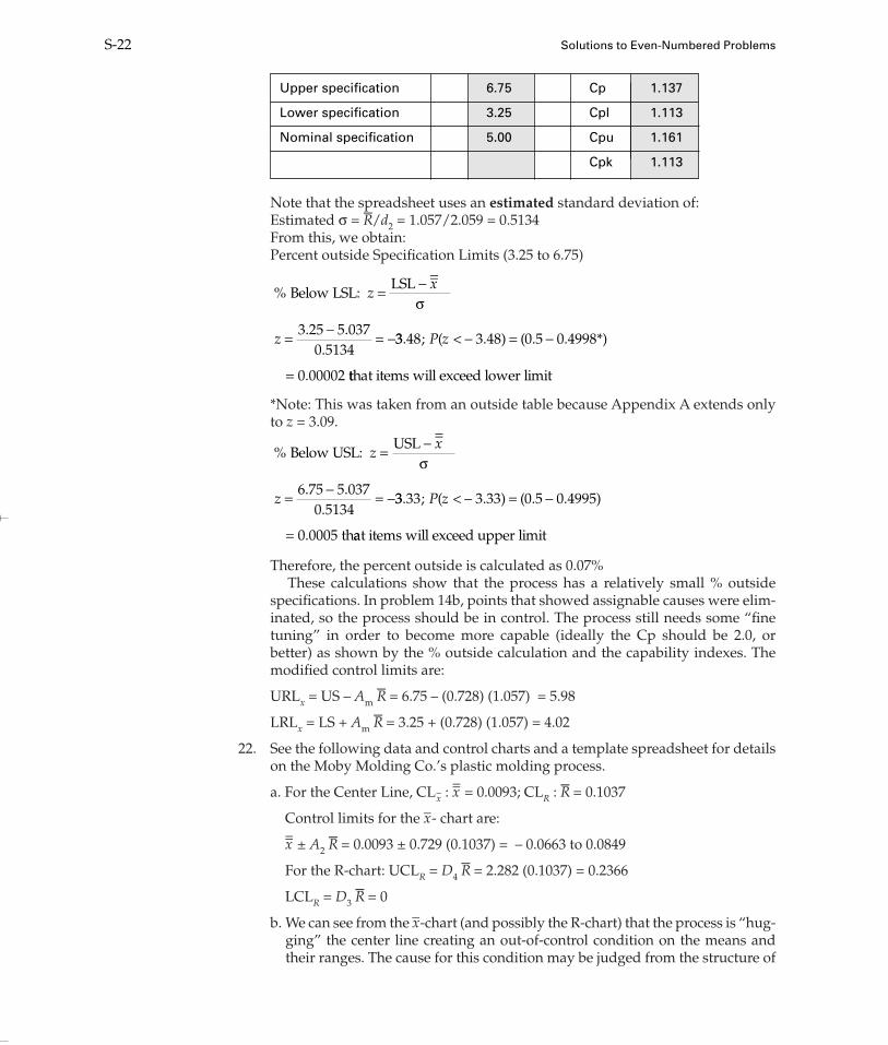
Note that the spreadsheet uses an estimated standard deviation of: Estimated σ = R–/d2 = 1.057/2.059 = 0.5134From this, we obtain:Percent outside Specification Limits (3.25 to 6.75)

*Note: This was taken from an outside table because Appendix A extends onlyto z = 3.09.

Therefore, the percent outside is calculated as 0.07% These calculations show that the process has a relatively small % outside

specifications. In problem 14b, points that showed assignable causes were elim-inated, so the process should be in control. The process still needs some “finetuning” in order to become more capable (ideally the Cp should be 2.0, orbetter) as shown by the % outside calculation and the capability indexes. Themodified control limits are:

URLx = US – Am R– = 6.75 – (0.728) (1.057) = 5.98

LRLx = LS + Am R– = 3.25 + (0.728) (1.057) = 4.02

22. See the following data and control charts and a template spreadsheet for detailson the Moby Molding Co.’s plastic molding process.

a. For the Center Line, CLx– : x= = 0.0093; CLR : R– = 0.1037

Control limits for the x–- chart are:

x= ± A2 R– = 0.0093 ± 0.729 (0.1037) = – 0.0663 to 0.0849


LCLR = D3 R– = 0

b. We can see from the x–-chart (and possibly the R-chart) that the process is “hug-ging” the center line creating an out-of-control condition on the means andtheir ranges. The cause for this condition may be judged from the structure of

%

. ..

Below USL:USL

zx

z

= − =

= − = −

σ

6 75 5 0370 5134

33 33 0 4995. ; .P z( < 3.33) (0.5 )

0.0005 th

− = −

= aat items will exceed upper limit

%

. ..

Below LSL:LSL

zx

z

= − =

= − = −

σ

3 25 5 0370 5134

33 48 0 4998. ; . *P z( < 3.48) (0.5 )

0.00002

− = −

= tthat items will exceed lower limit


Upper specification 6.75 Cp 1.137

Lower specification 3.25 Cpl 1.113

Nominal specification 5.00 Cpu 1.161

Cpk 1.113


the data. It appears that each of the heads on the molding machine has a sep-arate distribution of data. Thus, control charts should be prepared for eachhead, rather than treating the data as if it came from the same population.

24. See control charts for Wilmer Machine Co. and template spreadsheet for details.a. For the center line, CL x

– : = 3.526; CLs : s– = 0.359Control limits for the x–-s charts are:x= ± A3 s– = 3.526 ± 1.954 (0.359) = 2.825 to 4.227For the s-chart: UCLs = B4 s

– = 2.568 (0.359) = 0.922

LCLs = B3 s– = 0

The x– chart shows an out-of-control condition, with points 11 through 18 belowthe center line. Causes must be investigated and the process must be broughtunder control before x–-s charts can be used for process monitoring.

26. The data and control charts from the template spreadsheet show that.For the Hertz Co. data from problem 14-7, the center line, CLx

–:

x= = 400.290; CLs : s– = 16.404

Control limits for the x–- s charts are:

x= ± A3 s– = 400.290 ± 1.954(16.404) = 368.263 to 432.344

For the s-chart: UCLs = B4 s– = 2.089 (16.404) = 42.127

LCLs = B3 s– = 0

Because the revised data from problem 14-7 (b) with 23 samples was used, theprocess is under control, with no apparent problems.

28. Using data from problem 14, Slobay Co. as individual measures, with 5 samplemoving ranges, the calculations for the x-chart for individuals and R-chart show:From the data shown below, : x– = 0.0762; R– = 0.0050Control Limits on x:

UCLx = x– + 3 (R–/d2) = 0.0762 + 3 (0.0050)/2.326 = 0.0827

LCLx = x– – 3 (R–/d2) = 0.0762 – 3 (0.0050)/2.326 = 0.0698

Control limits on R: UCLR = D4R– = 2.114(0.0050) = 0.0106

LCLR = D3 R– = 0(0.0050) = 0

The process is probably out of control, with points 25–36 “hugging” the centerline on the x-chart and points 33–60 on the Moving Range Chart above thecenter line. Reasons for the out-of-control condition need to be sought out andcorrected.

30. Control limits for Yummy Candy Company are as follows:

Control limits:

UCLp = p– + 3 sp–

UCLp = 0.0333 + 3(0.0207) = 0.0954

CL

s p p n

s

p

p

p

= =

= −

=

75 2250 0 0333

1

0 0333

/

/

.

[( )( )]

( . ))( . )/ .0 9667 75 0 0207=



LCLp = p– – 3 sp–

LCLp = 0.0333 – 3(0.0207) = – 0.0288, use 032. The data and control chart for Quality Printing Company’s plant from the tem-

plate spreadsheet show:

CLp– = 0.06

Control limits:

UCLp = p– + 3 sp = 0.06 + 3(0.0336) = 0.1608

LCLp = p– – 3 sp = 0.06 – 3(0.0336) = – 0.0408 use 0

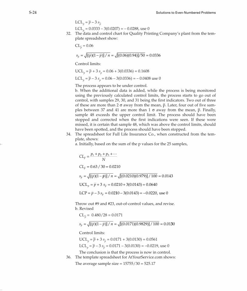
The process appears to be under control.b. When the additional data is added, while the process is being monitoredusing the previously calculated control limits, the process starts to go out ofcontrol, with samples 29, 30, and 31 being the first indicators. Two out of threeof these are more than 2 σ away from the mean, p–. Later, four out of five sam-ples between 37 and 41 are more than 1 σ away from the mean, p–. Finally,sample 48 exceeds the upper control limit. The process should have beenstopped and corrected when the first indications were seen. If these weremissed, it is certain that sample 48, which was above the control limits, shouldhave been spotted, and the process should have been stopped.

34. The spreadsheet for Full Life Insurance Co., when constructed from the tem-plate, shows:a. Initially, based on the sum of the p values for the 25 samples,

Throw out #9 and #23, out-of-control values, and revise.b. Revised

CLp– = 0.480/28 = 0.0171

Control limits:

UCLp = p– + 3 sp– = 0.0171 + 3(0.0130) = 0.0561

LCLp = p– – 3 sp– = 0.0171 – 3(0.0130) = −0.0219, use 0

The conclusion is that the process is now in control.36. The template spreadsheet for AtYourService.com shows:

The average sample size = 15755/30 = 525.17

s p p np = − = =[( )( )]/ [( . )( . )]/ .1 0 0171 0 9829 100 0 01330

CLp p p

N

CL

s p

p

p

p

= + + +

= =

= −

1 2 3

0 63 30 0 0210

1

�

. / .

[( )( pp n

pp

)]/ [( . )( . )]/ .= =

= +

0 0210 0 979 100 0 0143

3UCL . ( . ) .

.

s

p s

p

p

= + =

= − =

0 0210 3 0 0143 0 0640

0 02LCP 3 110 3 0 0143 0 0220− = −( . ) . , use 0

s p p np = − = =[( )( )]/ [( . )( . )] .1 0 06 0 94 50 0 0336/



CLp– = 202/15755 = 0.0128

UCLp = p– + 3 sp– = 0.0128 + 3(0.0049) = 0.0275

LCLp = p– – 3 sp– = 0.0128 – 3(0.0049) = – 0.0019, use 0

All points fall within the control limits.38. The template spreadsheet, using data from problem 14–34, can be used to con-

struct the np-chart for the Full Life Insurance Company, yielding the followingresults:

CLnp– = n p– = 100(0.021) = 2.1

Control limits:

UCL np– = np– + 3 snp

– = 2.1 + 3(1.434) = 6.402

LCL np– = np– – 3 snp

– = 2.1 – 3(1.434) = −2.202, use 0

As was shown in the previous control chart for problem 14-34, values for sam-ples 9 and 23 are out of limits. Eliminating these points, we get revised controllimits shown for the final control chart (follows). Note that the two values of 6or more were dropped.

Problem 38—Revised

So, CLnp– = np– = 100 (0.0171) = 1.71

Control limits:

UCLnp– = np– + 3 snp

– = 1.71 + 3(1.296) = 5.598

LCL np– = np– – 3 snp

– = 1.71 – 3(1.296) = −2.178, use 0

40. Center line for the c-chart: c– = 1000/40 = 25

42. Data for defects per pizza in a new store being opened by Rob’s Pizza Palaces isused to construct a c-chart. The chart shows:Number defective = 84; number of samples = 25Center Line for the c-chart: c– = 84/25 = 3.36

The process appears to be in control.44. For the c-chart: Center Line: c– (average number of defects) = 18

c c± 3 18 3(4.24) 18 12.72 5.28 to= ± = ± = 30 72.

c c± 3 3.36 3 3.36 = 3.36 5.50

= 2.14

= ± ±

− tto 8.86, use 0 for lower control limit.

c c± = ± = ± =3 to30 3 25 30 15 15 45

s n p pnp = − = =[ ( )( )] ( . )( . ) .1 100 0 0171 0 9829 1 296

s n p pnp = − = =[ ( )( )] ( . )( . ) .1 100 0 021 0 979 1 434

s p np = − = =[( )( )]/ [( . )( . )]/ .1 0 0128 0 9872 525 17 0p ..0049



46. The appropriate sample size for detecting shifts in means is simply an exercise inreading values from the curves to fit required conditions.a. For a 1 σ shift and a 0.80 probability, use n = 15 (if rounded to next higher value).b. For a 2 σ shift and a 0.95 probability, use n = 8 (rounded to next higher value).c. For a 2.5 σ shift and a 0.90 probability, use n = 3 (rounded to next higher value).

48. The stabilized p-chart diagram, based on the post office example, plots the“transformed z statistic” instead of p, and it shows the process is in control. Toverify calculations from the spreadsheet, for example, the first data point is:

Note that p– (1 – p–) is not divided by n because this is the estimated process stan-dard deviation, not the sample standard deviation. Thus variations in sampleand lot sizes can be tolerated here, where they might cause problems with thestandard p-chart.

50. The control chart for the EMWA versus observed values shows that, with anα = 0.8, the process is under control, and the EMWA estimate fairly closely antic-ipates the next observed value. The conclusion is that a better “forecast” of futurevalues may be obtained for volatile values such as these if a larger α value isused to give greater weight to more recent values.For problems 52 through 54, see the Statistical Foundations of Control ChartsSection in the Bonus Materials folder on the CD-ROM.

52.

Therefore, z0.02 = 1.64 or 1.65 because it is equidistant (0.4495 and 0.4505, respec-tively) between the closest table values to 0.4500.

54. Using the binomial formula:

Probability (acceptance) andx

n

= ==

∑ f x f xn

( ) (0

)) ( ) ( )

( . ) .

= −

= =

−x p px n x

in a row

1

11 0 5 0 0411 99

111110

0 5 0 5 11 0 510 1

%

( . ) ( . ) ( . )of 11 =

= 111

9 2

0 539

9119

0 5 0 5 55

=

=

=

. %

( . ) ( . ) (of 11 00 5 2 695

8118

0 5 0 5

11

8 3

. ) . %

( . ) ( . )

=

=

of 11 == =

=

165 0 5 8 085

7117

0 5

11

7

( . ) . %

( . ) (of 11 00 5 330 0 5 16 174 11. ) ( . ) . %= =

∴ 9 out of 11 pointss are statistically significant (p < 0.05)..

α2

0 102

0 05= =.. ; From the normal probability ttable, )P z( .= 0 4500

zp p

p

= − = − =σ

0 03 0 0220 1467

0 0545. .

..

p p p= = − = − =0 022 0 022 1 0 022 0 146. . ( . ) .σprocess

(1 ) 77



82286 16 solution - cengage 35,000 rework 70,000 correcting imperfections 6,250 rework due to vendor...

Documents