9 implications of air pollutant emissions from producing ......272 | 2016 billion-ton report 9.2...
TRANSCRIPT

2016 Billion-Ton Report | 269
9Implications of Air Pollutant Emissions from Producing Agricultural and Forestry Feedstocks
Ethan Warner,1 Yimin Zhang,1 Danny Inman,1 Annika Eberle,1 Alberta Carpenter,1 Garvin Heath,1 and Dylan Hettinger1
1 National Renewable Energy Laboratory, Golden, CO 80401-3305, USA

ImPlIcAtIons oF AIr PollutAnt EmIssIons From ProducIng AgrIculturAl And ForEstry FEEdstocks
270 | 2016 Billion-Ton Report
9.1 IntroductionMinimizing human health impacts is one tenet of sustainability. Human health problems associated with air pollution are not confined to urban areas. In fact, agricultural production is one of the largest contributors to the emissions of particulate matter and ozone precursors, which are regulated by the U.S. Environmental Protection Agency (EPA) due to their significant health (e.g., respiratory) and environmental (e.g., visibility, vegetation damages) impacts (EPA 2016c). Not surprisingly, across the biofuel supply chain, biomass production is one of the largest contributors to the emission of particulate matter and ozone precursors (Nopmongcol et al. 2011; Hill et al. 2009; Cook et al. 2011). In the context of air pollution, the magnitude combined with the spatial and temporal distribution are key to assessing the human health risks associated with a given emission source. Be-cause biomass production and supply systems vary spatially, temporally, and by the types of biomass used, the potential expansion of biomass supply systems to meet large-scale bioenergy demands could lead to substantial changes in air pollutant concentrations across the United States (DOE 2016; Hill et al. 2009; Cook et al. 2011; Tessum, Marshall, and Hill 2012; Andersen 2013; Yu et al. 2013; Tessum, Hill, and Marshall 2014; Zhang et al. 2016).
Air emissions from biomass production have been modeled previously (e.g., Andersen 2013; Nopmongcol et al. 2011; Hill et al. 2009; Tessum, Marshall, and Hill 2012; Tessum, Hill, and Marshall 2014; Tsao et al. 2011; Huo, Wu, and Wang 2009; Cook et al. 2011). However, modeling in the literature is limited with regard to assessing potential large-scale deployment of biomass supply systems envisioned for the near-term and long-term future (Andersen 2013). Only in the last few years have small-scale studies of emissions from potential future bio-mass-collection and -transportation systems been performed (e.g., Yu et al. 2013). Most studies evaluate current or past feedstock-supply systems (Nopmongcol et al. 2011; Andersen 2013; Hill et al. 2009; Tessum, Marshall, and Hill 2012; Tessum, Hill, and Marshall 2014); the exceptions being Tsao et al. (2011) and Huo, Wu, and Wang (2009)—both of which considered scenarios that are representative of future feedstock-supply systems. In addition to not representing anticipated future conditions for biomass production, many studies are limited in terms of the feedstocks evaluated, emissions assessed, and spatial resolution modeled.
Across the biomass supply chain, multiple operations emit air pollutants; however, the type and source of emissions varies by feedstock. Characteristics of emission sources, their locations, and their time signatures are essential pieces of information for air-quality and human health impact modeling. This analysis develops an emissions inventory of emission sources associated with biomass production and supply, which can serve as a foundation for a subsequent air pollutant concentration and human health impact analysis. Our analysis also allows for the identification of key factors that contribute to emissions, which can inform the development of mitigation options. However, our analysis does not evaluate potential change in ambient air quality that may result from the emissions associated with increased biomass feedstock production and supply.
2016 Billion-Ton Report | 271
The objectives of this analysis of air pollutant emis-sions implications from potential biomass production and logistics from the three BT16 scenarios (see chapter 2) are to:
• Quantify air pollutant emissions associated with select scenarios of potential biomass produc-tion, harvest, transportation, and preprocessing that align with the select scenarios described in chapter 2 of this volume and compare emissions among feedstocks
• Estimate the spatial distribution of modeled air emissions and assess how these changes could potentially impact local air quality
• Identify opportunities to minimize potential ad-verse impacts, given that the design of the entire supply chain for primarily cellulosic biomass is still in its infancy.
Assessing the change to air pollutant emissions attributed to future potential biomass production requires the estimation of emissions for both a future scenario and a reference scenario, as well as the difference between the two. The scenarios analyzed in this study are consistent with those in the rest of BT16 volume 2. However, in the context of this study, the reference scenario would need to include emissions from local agricultural and forestry sourc-es, as well as other important sources of emissions, such as transportation. BT16 lacks the detailed char-acterization of such a reference scenario; therefore, we report estimates of mass emissions for the scenar-ios evaluated and compare our results to EPA’s most recent National Emissions Inventory (NEI) of U.S. air pollutant emissions (EPA 2016d).
The methods employed to achieve the stated ob-jectives expand on those developed in Zhang et al. (2016) for estimating inventories of air pollutant emissions from potential biomass production. Key
enhancements to the Zhang et al. methods are that we developed a method to estimate air emissions associated with biomass feedstock transportation and preprocessing. We also included new feedstock types and adopted crop budgets at higher spatial resolu-tion than were available in the previous databases from Zhang et al. We updated assumptions regarding biomass production and harvest to ensure consistency with those in BT16 volume 1. BT16 focuses on the supply chain stages of producing biomass and sup-plying a subset of that biomass to the reactor throat of a biorefinery; biomass conversion to energy (e.g., biofuels) and biofuel combustion in vehicles are not a part of this analysis. This chapter does not take land management change results from BT16 volume 1 and chapter 3 and estimate net changes in emissions.
Our inventory approach allows for an assessment of potential biomass feedstock production and logistics scenarios as compared to a set of baseline conditions. In particular, this chapter focuses exclusively on esti-mating air emissions from biomass supply systems to
• Understand how emissions differ among various biomass feedstocks and by location (i.e., coun-ties in the contiguous United States), and how these emissions may evolve over time under different scenarios
• Identify the major emission contributors along the biomass supply chain in order to inform emission-mitigation strategies
• Compare the magnitude of feedstock-related emissions to county-level emissions (derived from EPA’s NEI) to identify geographic areas at higher risk for potential negative air quality impacts, for instance, for those counties current-ly not in compliance with National Ambient Air Quality Standards (NAAQS) as of 2015.

ImPlIcAtIons oF AIr PollutAnt EmIssIons From ProducIng AgrIculturAl And ForEstry FEEdstocks
272 | 2016 Billion-Ton Report
9.2 MethodsCounty-level air pollutant emissions are estimated from anthropogenic sources for each of the three BT16 scenarios described in table 9.1 and section 9.2.1. These scenarios are for 2017 (agricultural base case yield growth [BC1] and the moderate housing–low wood energy [ML] forestry scenarios combined: BC1&ML 2017) and 2040 (BC1&ML 2040, high-yield growth [HH3] and the high housing–high wood energy [HH] scenarios combined: HH3&HH 2040). The air pollutants analyzed are carbon monoxide (CO), particulate matter (PM2.5, PM10), oxides of nitrogen (NOX),1 oxides of sulfur (SOX),2 volatile or-ganic compounds (VOCs),3 and ammonia (NH3). Air pollutants emitted from fuel used by equipment (e.g., agricultural machinery, transport vehicles); fertilizer and pesticide (collectively referred to as “chemicals”) applications; soil and plant matter disturbance by mechanical force (e.g., wheels); and feedstock-drying processes (if applicable) are quantified.
Our analysis is focused on modeling direct, local air pollutant emissions. Indirect upstream emissions associated with fuel and chemical production are not included in this analysis, but they are discussed in section 9.3.4.1 in reference to the estimated emis-sions inventory. In addition, biogenic pollutants such as VOCs from biomass vegetation and cutting of biomass during harvest are not included, with one exception—VOC emissions from feedstock prepro-cessing and drying are included as they are biogenic emissions induced through an anthropogenic indus-trial process. Furthermore, we do not assess avoided emissions due to displacing production and extraction of fossil fuel (the part of the fossil fuel supply chain equivalent to biomass production). These limitations are discussed further in sections 9.3.4 and 9.4.2.
9.2.1 Scope of the AnalysisOur analysis is focused on developing air pollutant emissions inventories for three potential biomass production and harvest (hereafter referred to as “production”) scenarios and three potential biomass feedstock transportation and preprocessing (hereafter referred to as “supply logistics”) scenarios that align with the select scenarios evaluated in other chapters of this volume; complete scenario descriptions can be found in chapter 2. These scenarios are based on biomass production and supply logistics from BT16 volume 1, and they include BC1&ML 2017 (near-term supply logistics to deliver bales or wood chips to the biorefinery), BC1&ML 2040 (long-term supply logistics to transform raw biomass to a pelletized commodity), and HH3&HH 2040 (long-term supply logistics). Each biomass production scenario corre-sponds to a supply logistics scenario, but energy crop production in the potential biomass production sce-nario for 2017 is expected to be zero because BT16 volume 1 had reported that no crops were established in 2017, and the supply of conventional crops (e.g., corn grain) to biorefineries was not modeled. Volume 1 had reported that no crops were established in 2017 and the supply of conventional crops (e.g., corn grain) to biorefineries was not modeled.
Model inputs to estimate air emissions for these scenarios include three sets of data: (1) regional equipment use and chemical application budgets for biomass production; (2) county-level biomass production data; and (3) supply logistics data for the subset of produced biomass supplied to biorefineries (including equipment, biomass transportation dis-tance, and quantity of biomass). In a given county, potential biomass produced (e.g., all wheat straw and corn grain) may not be used for biofuel production in the BT16 scenarios used in this chapter. The data sets are derived from BT16 volume 1 or are in agreement
1 This includes nitric oxide and nitrogen dioxide.2 This primarily includes sulfur dioxide, but it also includes other oxides of sulfur, such as sulfur monoxide and sulfur trioxide.3 The list of VOCs accounted for from EPA methods and data sources are documented by EPA (2015a).
2016 Billion-Ton Report | 273
Figure 9.1 | Potential Biomass Production and Supply Logistics Scenarios from BT16 Volume 1 Evaluated in This Chapter
Feedstock TypeSegment of the Supply Chain
BC1&MLa HH3&HHb
2017 2040 2040
Corn Grain
Biomass ProductionUp to $60/dry ton (dt)
Up to $60/dt Up to $60/dt
Biomass Supply Logistics, Near-Term
NMc NM NM
Biomass Supply Logistics, Long-Term
NM NM NM
Cellulosic Agricultural Residues, Energy
Crops, Whole-Tree Biomass and
Logging Residues
Biomass Production Up to $60/dt Up to $60/dt Up to $60/dt
Biomass Supply Logistics, Near-Term
Up to $100/dtd
NM NM
Biomass Supply Logistics, Long-Term
NMUp to $100/
dtd Up to $100/dtd
a BC1&ML scenarios assume 1% yield growth per year.b HH3&HH scenario assume 3% yield growth per year.c Not modeled (NM) as a part of BT16.d Includes the cost to produce and supply the biomass.
with assumptions and inputs used to generate results in volume 1 (refer to section 9.2.2). Emissions for each scenario are estimated for all counties within the contiguous United States.
Table 9.2 presents the potential availability of bio-mass at a mean market clearing price of $60 per dry ton (dt) for years 2017 and 2040. We estimate emissions that would occur for biomass from the agriculture and forestry sectors listed in table 9.2. In this chapter we evaluate all cellulosic feedstocks po-tentially produced in 2017 and about 90% of cellulos-ic feedstocks potentially produced in 2040. In 2040 we do not evaluate the following: biomass sorghum, energy cane, eucalyptus, pine, poplar, or willow. We consider corn grain (Zea mays L.) because it is currently the most commonly used conventional
crop for biofuel production in the United States; it is used as a point of comparison for all other biomass feedstocks assessed in this study. For the purposes of this analysis, we aggregate some feedstocks into a single category based on equipment similarities and low production volume as indicated in table 9.2. For example, corn stover and sorghum stubble are aggre-gated into the “stover” category, whereas corn grain, switchgrass, and miscanthus are all kept as separate categories.
The dimensionality in equipment and chemical application budgets for whole-tree forestry biomass (hereafter referred to as “whole-tree biomass”) and logging residues vary by wood type, location, stand type, etc. (DOE 2016). Whole-tree biomass and log-ging residues are tracked separately because residue
4 For example, this includes fertilizer and pesticide application rates, equipment types, equipment operation type (e.g., harvest), equipment hours of operation per unit of biomass or acre, and equipment horsepower.
ImPlIcAtIons oF AIr PollutAnt EmIssIons From ProducIng AgrIculturAl And ForEstry FEEdstocks
274 | 2016 Billion-Ton Report
Table 9.2 | Potential Biomass-Production Levels (in dt) Evaluated in This Chapter
budgets only include chipping and loading of the bio-mass at the roadside. To simplify our results within a county across budget dimensionality, we aggregated the emissions for all stand types and wood types, such as hardwoods, softwoods, and mixedwoods, into whole-tree biomass and logging residues categories for each county.
Biomass production scenarios represent total poten-tial production at a mean market clearing price of $60 per dt regardless of use (i.e., includes biomass for all markets). Biomass supply responds to economic signals from several markets, and thus, biomass for biofuel is but one potential market for the biomass
grown. Biomass supply logistics scenarios repre-sent the potential supply of a subset of the biomass produced at a cost of up to $60 per dt that meets an average cost of up to $100 per dt delivered to biore-fineries for biofuel production.
Potential agricultural residues and energy crop biomass production would increase from 2017 to 2040. However, due to the BT16 assumption that no additional land will be used for forestry and that there will be no expansion of planted forest into “natural” forestland, logging residues biomass production would decrease from 2017 to 2040.
Biomass Feedstock Description
Biomass Feedstock Categories in This Chapter
BC1&MLa (million dt yr-1)
HH3&HHb (million dt yr-1)
2017 2040 2040
Conventional Agricultural Crop
Corn grain Corn grain 390 450 510
Subtotal 390 450 510
Agricultural Residuesc
Corn stoverStover
89 150 160
Sorghum stubble 0.71 1.1 1.5
Wheat straw
Straw
13 21 37
Barley straw 0.41 0.57 0.48
Oats straw 0.0049 0.0081 0.0066
Subtotal 100 180 200
Energy Cropsd
Miscanthus Miscanthus 0 160 370
Switchgrass Switchgrass 0 160 190
Subtotal 0 320 560
2016 Billion-Ton Report | 275
Biomass Feedstock Description
Biomass Feedstock Categories in This Chapter
BC1&MLa (million dt yr-1)
HH3&HHb (million dt yr-1)
Forestry Biomass
Hardwood Trees
Whole-Tree Biomass
39 25 18
Softwood Trees 28 33 20
Mixedwood Trees 2.8 2.4 2.4
Hardwood Residues
Logging Residues
6.9 8.0 7.9
Softwood Residues 6.8 10 9.6
Mixedwood Residues 4.2 2.7 2.4
Subtotal 88 81 61
Grand Total 590 1,000 1,300
a BC1&ML scenarios assume 1% yield growth per year.b HH3&HH scenarios assume 3% yield growth per year.c Agriculture residues include current feedstocks with production quantities available as bioenergy feedstocks.d Dedicated energy crops are feedstocks that are not currently in production but are expected to be available as bioenergy feed-
stocks in the future.
9.2.2 Description of Feedstock Production Emissions to Air Model (FPEAM)The National Renewable Energy Laboratory’s (NREL’s) FPEAM (fig. 9.1) is developed in Python v2.7.11 (Python Software Foundation 2016) and joins data and models from many disparate sources, dis-cussed below, to estimate anthropogenic air emissions from the sources and supply chain stages described in the previous section. FPEAM uses input and output data from the Policy Analysis System (POLYSYS) model, Forest Sustainable and Economic Analysis Model (ForSEAM), and the Supply Characterization Model (SCM) to estimate air pollutant emissions of CO, PM2.5, PM10, NOX, SOX, VOCs, and NH3. FPEAM uses regional equipment and chemical application data that are inputs to these models, biomass pro-duction estimates that are outputs from POLYSYS and ForSEAM, and biomass supply to the biorefin-
ery estimates that are outputs from SCM. Input and output data from POLYSYS, ForSEAM, and SCM are generated externally and provided as model inputs to FPEAM simulations. Section 9.2.2.1 provides an over-view of the scope of included emissions and emission sources. Section 9.2.2.2 describes FPEAM emission estimation methods, with details included in appendix 9-A section 9A.1, and section 9.2.2.3 summarizes the FPEAM outputs.
FPEAM’s core methods for estimating emissions inventories are based on Zhang et al. (2016). However, FPEAM was expanded and improved for this chapter’s analyses by including additional biomass feedstocks (e.g., miscanthus, whole-tree biomass) and emissions from the biomass supply logistics system. In this chapter, we reproduce documentation of many of the methods in Zhang et al. (2016) to ensure they are clear, as there have been many small changes to FPEAM to both update datasets and better align our analysis with the BT16 study.
ImPlIcAtIons oF AIr PollutAnt EmIssIons From ProducIng AgrIculturAl And ForEstry FEEdstocks
276 | 2016 Billion-Ton Report
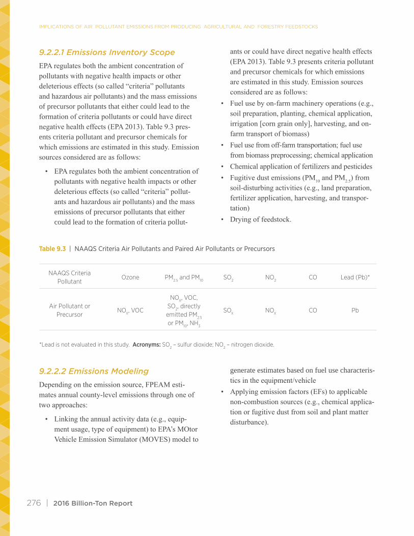
Table 9.3 | NAAQS Criteria Air Pollutants and Paired Air Pollutants or Precursors
9.2.2.1 Emissions Inventory Scope
EPA regulates both the ambient concentration of pollutants with negative health impacts or other deleterious effects (so called “criteria” pollutants and hazardous air pollutants) and the mass emissions of precursor pollutants that either could lead to the formation of criteria pollutants or could have direct negative health effects (EPA 2013). Table 9.3 pres-ents criteria pollutant and precursor chemicals for which emissions are estimated in this study. Emission sources considered are as follows:
• EPA regulates both the ambient concentration of pollutants with negative health impacts or other deleterious effects (so called “criteria” pollut-ants and hazardous air pollutants) and the mass emissions of precursor pollutants that either could lead to the formation of criteria pollut-
ants or could have direct negative health effects (EPA 2013). Table 9.3 presents criteria pollutant and precursor chemicals for which emissions are estimated in this study. Emission sources considered are as follows:
• Fuel use by on-farm machinery operations (e.g., soil preparation, planting, chemical application, irrigation [corn grain only], harvesting, and on-farm transport of biomass)
• Fuel use from off-farm transportation; fuel use from biomass preprocessing; chemical application
• Chemical application of fertilizers and pesticides• Fugitive dust emissions (PM10 and PM2.5) from
soil-disturbing activities (e.g., land preparation, fertilizer application, harvesting, and transpor-tation)
• Drying of feedstock.
NAAQS Criteria Pollutant
Ozone PM2.5 and PM10 SO2 NO2 CO Lead (Pb)*
Air Pollutant or Precursor
NOX, VOC
NOX, VOC, SO2, directly emitted PM2.5
or PM10, NH3
SOX NOX CO Pb
*Lead is not evaluated in this study. Acronyms: SO2 – sulfur dioxide; NO2 – nitrogen dioxide.
9.2.2.2 Emissions Modeling
Depending on the emission source, FPEAM esti-mates annual county-level emissions through one of two approaches:
• Linking the annual activity data (e.g., equip-ment usage, type of equipment) to EPA’s MOtor Vehicle Emission Simulator (MOVES) model to
generate estimates based on fuel use characteris-tics in the equipment/vehicle
• Applying emission factors (EFs) to applicable non-combustion sources (e.g., chemical applica-tion or fugitive dust from soil and plant matter disturbance).

2016 Billion-Ton Report | 277
Figure 9.1 | FPEAM Model (orange shade) summary of the linkages between primary inputs (blue shade), emission estimation models and methods (gray boxes) used in or with FPEAM (orange boxes), and analysis results (green shades)
INPUTS
RESULTS
FPEAM
POLYSYS and ForSEAMinputs and outputs
Biomass Production budgets, production,
and harvest areas
Mass emission per dry ton feedstock
Production activityCounty-level equipment use and
fertilizer application
Non-point emissionsChemical application
and fugitive dust
On-roadFuel-use emissions
Non-roadFuel-use emissions
Point emissionsWoody biomass drying
and preprocessing
Supply logisitics activityCounty-level equipment use
Other data sources
Corn grain irrigation statistics, EPA guidance and technical
reports, and literature
Source contributions to total emission
SCM inputs and outputs
Biomass supply logistics budgets and supply to
biorefineries
Comparison to NEI and attainment status
County-level mass-emission density maps
EPA NONROAD model
Emission factor-based calculation
Emission factor-based calculation
EPA MOVES model
Figure 9.1 summarizes the interlinkages between the primary FPEAM inputs and air pollutant estimation methods to generate model outputs (i.e., county-level air emissions). Table 9.4 builds on this by summa-rizing the sources and scope of the core elements of
FPEAM’s methods for estimating emissions. See below for a brief description of table 9.4. See appen-dix 9-A section 9A.1.1 for more details on estimating annual activity and see appendix 9-A section 9A.1.2 for greater details on EFs and total emissions estimation.

ImPlIcAtIons oF AIr PollutAnt EmIssIons From ProducIng AgrIculturAl And ForEstry FEEdstocks
278 | 2016 Billion-Ton Report
Annual activity of equipment (e.g., hours of opera-tion per year) and chemical application that would be associated with each county under each scenario are estimated based on BT16 volume 1. These data are based on the biomass production and supply logistics budgets used as inputs to POLYSYS, ForSEAM, and SCM. They are also based on POLYSYS and ForSEAM estimates of potential harvested area and biomass production, and SCM estimates of poten-tial biomass supply (DOE 2016). Our method also considers the use of irrigation equipment for corn grain-based irrigation based on data from the U.S. Department of Agriculture (USDA) (USDA 2009).
In alignment with BT16 budget data, product-pur-pose-based allocation is assumed for allocating emissions among multi-product production systems, such as those generating residues as byproducts (Johnson et al. 2004; Wang, Huo, and Arora 2011). Equipment operations associated with biomass pro-duction are entirely attributed to grain or wood rather than residues; in agriculture, harvest activities are allocated between the crop and agricultural residue; and additional chemical and nutrient applications (to compensate for nutrient loss) are attributed to stover, straw, or logging residues.
Switchgrass and miscanthus are perennial crops with 10- and 15-year production cycles, respectively; each with differing equipment budgets for each rotation year. To compare them to annual crops, we annu-alize emissions from equipment use and chemical application over all rotation years for these crops by assuming 10% of total switchgrass and 6.67% of miscanthus acres are in production in each rotation year in each county. Year-to-year emissions may be more variable depending on where the crops are in the rotation cycle.
For air pollutant emissions that would be generated by mobile and non-mobile equipment, emissions are estimated in FPEAM by using EPA’s MOVES Model version 2014a (EPA 2016a). For non-road equipment, the MOVES Model relies on the submodel NON-
ROAD 2008a (EPA 2016b; hereafter referred to as NONROAD) to compute county-level air pollutant emissions for machinery like combines, tractors, and chippers. In addition, the main MOVES Model uses county-level EFs to compute county-level air pollut-ant emissions from on-road machinery such as trucks. While MOVES estimates CO, NOX, SOX, PM10, PM2.5, NH3, and VOCs emissions directly, NON-ROAD only calculates CO, NOX, SOX, PM10, and total hydrocarbon (THC) emissions. As a result, for NONROAD equipment, we estimate the emissions of NH3, PM2.5, and VOCs using EPA EFs based on fuel consumption, THCs, and PM10, respectively (see appendix 9-A section 9A.2.1 for further details).
Transportation distance for potential biomass sup-plied to biorefineries is determined using the SCM (DOE 2016). While on-road transportation emissions are being estimated at a county level, we do not have the necessary pathing (i.e., course routing) data for specific biomass streams. As a result, all on-road transportation emissions are allocated to the county producing the biomass.
NH3 and NOX (in the form of NO) emissions from the application of nitrogen (N) fertilizers are estimated based on EFs specific to each fertilizer and pollutant (EPA 2015d; Hall and Matson 1996; Veldkamp and Keller 1997; Goebes, Strader, and Davidson 2003). For the pollutants examined, no EFs for the appli-cation of potassium and phosphorus fertilizers were found, so this analysis excludes emissions that would be generated by these fertilizers.
Fugitive dust is PM2.5 and PM10 that is emitted from the mechanical disturbance of granular material (typ-ically soil and plant matter) exposed to the air and from mechanical systems preprocessing operations (chipper, hogs, tubs, etc.) (USDA 2011; EPA 2006). This kind of dust is called “fugitive” because it is not created in a confined flow stream. Typical sources of fugitive dust include unpaved roads, agricultural tilling operations, aggregate storage piles, and heavy construction operations. Dust is typically generated

2016 Billion-Ton Report | 279
by two basic physical phenomena: (1) pulverization and abrasion of surface materials by applying me-chanical force with implements (wheels, blades, etc.); and (2) entrainment of dust particles by the action of turbulent air currents, such as the wind erosion of an exposed surface. No methods for estimating fugitive dust from forestry activities were found, so we assume fugitive dust emissions are zero. There is evidence that this gap may not have a significant impact on our results because research has shown that vegetation in forested areas can potentially remove 80%–100% of particulate emissions (Pace 2005). Fugitive dust from preprocessing equipment was assumed to be zero because of the dust collection systems included in both near-term and long-term supply logistics designs (INL 2013; INL 2014).
Drying woody biomass is the main approach for lowering the moisture content of the biomass in both near-term and long-term supply logistics designs (INL 2013; INL 2014). During the drying process, biogenic VOC emissions would be expected to be emitted to the air (EPA 2002), and they are account-ed for in our emissions inventory. Due to the limits of the available data on herbaceous feedstocks (e.g., EPA 1996), we assume there are no VOC emissions from herbaceous feedstock drying. We do not include other biogenic related air pollutant emissions, for
instance, from the growth of herbaceous or woody feedstocks.
Logging residues are sometimes piled and burned. The use of this practice varies based on a number of factors, including ownership, location, type, regen-eration, and forest productivity. Because we did not have access to spatial data on specific logging residue management practices, this analysis does not estimate any credits from the offsetting of burning logging residues.
Although we do not include upstream emissions in the study, we do discuss potentially large sources of upstream emissions and present example estimates that could be expected, such as upstream emissions from biomass preprocessing equipment that con-sumes electricity. These results are presented and discussed in sections 9.3.4.1 and 9.3.4.2, respectively. Emissions from electricity use would not be local, and even the general location of their release would be difficult to pinpoint. In section 9.3.4.3, we discuss a sensitivity estimate of emissions assuming 99%, rather than 100% dust collection and compare it to other sources of PM emissions. In section 9.4.2, we discuss other important shortcomings of our approach and methods, such as the limitations in evaluating fugitive dust emissions and biogenic emissions from forestry and open burning of whole-tree biomass.

ImPlIcAtIons oF AIr PollutAnt EmIssIons From ProducIng AgrIculturAl And ForEstry FEEdstocks
280 | 2016 Billion-Ton Report
Table 9.4 | FPEAM Model Summary and Documentation of Methods
PurposeFPEAM
Modeling Method
Emission Species
Spatial Resolution
Estimation Methods/Data Sources
Details in Appendix Section
Annual Equipment Usage and Chemical
Application
Equipment and Chemical Application
Budgetsa
CO, NOX, SOX, PM2.5, PM10, VOCs, NH3
Agriculture 13 regional budgets
Forestry 5 regional budgets
Supply Logistics National
Corn Grain Irrigation State
POLYSYS, ForSEAM, and SCM
modeling inputs (DOE 2016)
Corn Grain Irrigation
USDA (2007)
9A.1.1
Harvest Area and Biomass Production
CO, NOX, SOX, PM2.5, PM10, VOCs, NH3
County
POLYSYS, ForSEAM, and SCM
modeling output (DOE 2016)
9A.1.1
Emission Factors (EFs)
For Estimating
Annual Emissions
Off-Road Fuel Use
CO, NOX, SOX, PM2.5, PM10, VOCs, NH3
State EFsNONROAD
(EPA 2016b)9A.1.2.1
On-Road Fuel Use
CO, NOX, SOX, PM2.5, PM10, VOCs, NH3
State EFsMOVES
(EPA 2016a)9A.1.2.2
Preprocessing Fuel Use
CO, NOX, SOX, PM2.5, PM10, VOCs, NH3
State EFsNONROAD
(EPA 2016b)9A.1.2.3
Chemical Application
NOx, VOCs National EFs
EPA (2015c) ANL 2015
USDA (2010) Davidson et al. 2004
Huntley (2015)
9A.1.2.4
Fugitive Dust PM2.5 and PM10
EFs based on a com-bination of state and
national data
Agriculture Harvest and Non-Harvest
CARB (2003), Gaffney and Yu (2003)
Forestry No methodology or data could
be found
Transportation EPA (2006)
Preprocessing None due to dust-collection
equipment (INL 2013; INL 2014)
9A.1.2.5
Drying and Preprocessing
VOCs National EFs
Herbaceous: Assumed to be zero
Woody: EPA (2002)
9A.1.2.6
a Budgets include additional dimensions not described here (e.g., budgets by tillage type, rotation year for energy crops, and forestry land type).

2016 Billion-Ton Report | 281
9.2.2.3 Emission Metrics
Three metrics were used in this study to provide insights about the differences in emissions from potential feedstock production, sources of emissions, and the comparison to historic emissions:
• Air pollutant emissions per unit of biomass pro-duced or supplied, which are used to compare corn grain and cellulosic feedstocks (section 9.2.2.3.1)
• Percent contribution of emissions by activity type to identify the activities that contribute most to the emissions of each pollutant (section 9.2.2.3.2)
• Ratios of emissions from BT16 scenarios and current national emissions inventories, specif-ically the 2011 NEI and NAAQS 2015 attain-ment status (section 9.2.2.3.3).
9.2.2.3.1 Emission By Feedstock
The metric of air pollutant emissions per unit of biomass produced or supplied is calculated as a ratio. For biomass produced in BT16 scenarios, the numera-tor is the sum of county-level mass emissions associ-ated with the production of a given feedstock, and the denominator is calculated based on the county-level feedstock produced. For biomass supplied to biorefin-eries in BT16 scenarios, the numerator is the sum of county-level mass emissions associated with the sup-ply of a given feedstock, and the denominator is the mass of a given feedstock supplied in a given county.
9.2.2.3.2 Contribution of Emissions by Activity Category
For each feedstock, we estimate and compare the relative contribution of each of five activity catego-ries (described below) to the total aggregated emis-sions from biomass production. Relative contribution is determined at a county level and displayed as national distributions of county-level emissions for each feedstock and pollutant. This metric provides
insight into which activities are major contributors to certain air pollutant emissions, which can help focus future research on mitigation strategies, as well as the variability of contribution which can suggest mitiga-tion strategies. Below, we detail how emissions are aggregated for each of the five categories:
• Non-Harvest Emissions:5 ▪ Fuel use-related emissions from machinery
operations associated with chemical applica-tion and field preparation (e.g., cultivating, discing, plowing, and irrigation)
▪ Fugitive dust emissions from non-harvest equipment usage.
• Chemical Application Emissions:6
▪ NH3 and NOX from nitrogen fertilizer appli-cation
▪ VOC emissions from pesticide application.
• Harvest Emissions: ▪ Fuel use and fugitive dust emissions from
machinery operations (e.g., mower, rake, baler) associated with feedstock harvesting
▪ Fuel use and fugitive dust emissions from equipment used to transport feedstock to a temporary on-farm storage facility
▪ Fuel use emissions from loading biomass for on-road transportation
▪ Fuel use emissions from preprocessing equipment used at the site of harvest (e.g., wood chipper).
• On-Road Transport Emissions: Fuel use and fugitive dust emissions from transporting feed-stocks to biorefineries by truck from the farm to the depot and/or biorefinery depending on the type of logistics system.
• Preprocessing Emissions: VOC emissions from preprocessing and drying at the facility.
For biomass produced, equation 9.1 calculates the contribution of each individual biomass production activity (non-harvest, chemical application, and har-
5 No methods for estimating fugitive dust from forestry activities were found so we assume fugitive dust emissions are zero.6 Note that for fertilizer and chemical applications, the fuel use and fugitive emissions associated with applying the fertilizers/chem-
icals are accounted for in the non-harvest activity category.

ImPlIcAtIons oF AIr PollutAnt EmIssIons From ProducIng AgrIculturAl And ForEstry FEEdstocks
282 | 2016 Billion-Ton Report
Equation 9.2:
Production Activity Contributionp = Σ emissions by activity
∑ emissions across biomass production activities
Production and Transporation Contributionp = Σ emissions by activity
∑ emissions across all activities
vest) to the overall emissions from potential biomass production. The ratio is computed by pollutant (p) and by feedstock, for each county, which produces a given feedstock.
As stated in section 9.2.1, only a subset of biomass produced would be supplied to biorefineries in the
scenarios examined as a part of BT16. Therefore, in a given county, potential biomass produced may not be used for biofuel production (DOE 2016). For biomass, which is produced and supplied to biore-fineries, equation 9.2 calculates the contribution of each individual activity to overall emissions from all feedstock production and supply-related activities.
Equation 9.1:
9.2.2.3.3 Comparison to NEI and Attainment Status for NAAQS
Our air pollutant emissions inventory is compared to the county-level NEI for 2011 to illustrate the mag-nitude of emissions from BT16 biomass production and supply logistics scenarios relative to inventoried emissions in a county. The NEI is a comprehensive and detailed estimate of air emissions of criteria pol-lutants, criteria precursors, and hazardous air pollut-ants from air emissions sources (EPA 2016d). Every 3 years, EPA publishes a NEI of air pollutant emis-sions for regulatory and air quality-modeling pur-poses (EPA 2016d). The NEI is based primarily upon data provided by state, local, and tribal air agencies for sources in their jurisdictions and supplemented by data developed by the EPA (EPA 2016d). The NEI for 2011 was the most recent at the time of the analysis for this report. Emissions in the NEI are provided
at the county level and categorized broadly as point (PT) or nonpoint (NP) for stationary sources, and on-road (OR) or non-road (NR) for mobile sources (EPA 2016d):
• PT sources include larger sources that are locat-ed at a fixed, stationary location.
• NP sources include emissions estimates for sources that individually are too small in magni-tude to report as point sources.
• OR sources include emissions from on-road ve-hicles that use gasoline, diesel, and other fuels.
• NR sources include off-road mobile sources that use gasoline, diesel, and other fuels.
Emissions from non-harvest and harvest activities belong to the NP and NR categories. Emissions from chemical-application emissions fall under the NP category. For biomass supplied to biorefineries, emis-

2016 Billion-Ton Report | 283
sions from on-road transportation fall under the OR category, while emissions from preprocessing belong to the PT category.
We construct ratios (R) that represent comparisons of the total mass of relevant direct and/or precursor emissions of criteria air pollutants from the scenarios (see table 9.3) to 2011 emissions of the same pollut-ants (from the 2011 NEI) and term these “emission ratios.” Estimated ratios (equations 9.3–9.8) from mass emissions are intended solely as comparisons to show how the magnitudes of criteria air pollutant (or precursors to criteria air pollutant) emissions from the BT16 scenarios compare to the baseline emissions. The emission ratios do not account for the temporal profiles and chemical speciation for each emission source that are necessary to understand potential changes in air quality. Therefore, these ratios are not meant to predict changes in ambient air quality (e.g., ozone, PM2.5 concentrations). However, because man-aging air quality must start with controlling emis-sions from the sources, these ratios could be useful in identifying areas of concern for local air quality management. See section 9.4.2 for further discussion of the limitations of our results to predict impacts on air quality.
Some criteria air pollutants are emitted directly by sources (e.g., CO); some are formed in the atmo-sphere (like ozone) through chemical reactions of pollutants directly emitted (called precursor pol-lutants); and some are generated both directly and indirectly (e.g., PM2.5, PM10, and SOX). The emission ratios for precursors to ozone, PM2.5/PM10, as well as sulfur dioxide (SO2), nitrogen dioxide (NO2), and
CO emissions are calculated using equations 9.3–9.8, respectively, and are reported in maps for all counties with cellulosic biomass feedstocks produced.
Emissions from non-harvest and harvest activities belong to the NP and NR categories. Emissions from chemical-application emissions fall under the NP category. For biomass supplied to biorefineries, emis-sions from on-road transportation fall under the OR category while emissions from preprocessing belong to the PT category.
The Clean Air Act requires EPA to set NAAQS for pollutants considered harmful to public health and the environment and identifies two types of these stan-dards. Primary standards provide public health pro-tection, including protecting the health of “sensitive” populations such as asthmatics, children, and the elderly. Secondary standards provide public welfare protection, including protection against decreased visibility and damage to animals, crops, vegetation, and buildings.
It can also be useful to place air pollutant emission estimates within the context of counties that are cur-rently not in compliance with the NAAQS for criteria pollutants, as determined and published by EPA (EPA 2015d; EPA 2016c) and labeled as nonattainment areas (NAAs).7 The concentrations of certain crite-ria pollutants are affected by emissions upwind, so we visually display all counties with emission ratios alongside those counties currently in nonattainment for applicable NAAQS. The locations of NAAs for 8-hr ozone, PM2.5, SO2, and PM10 NAAQS in 2016 are overlaid on the maps of the emission ratios in
7 A nonattainment area is defined as any area that does not meet (or that contributes to ambient air quality in a nearby area that does not meet) the national primary or secondary ambient air quality standard for the pollutant (EPA 2016d; EPA 2016c).

ImPlIcAtIons oF AIr PollutAnt EmIssIons From ProducIng AgrIculturAl And ForEstry FEEdstocks
284 | 2016 Billion-Ton Report
Equation 9.4:
Equation 9.5:
Equation 9.6:
Equation 9.7:
Equation 9.8:
Equation 9.3:
∑(NOx,SOx, NH3, PM2.5, and VOC)all activities
∑(NOx,SOx,NH3, and PM2.5)NEI NR +NP+OR + ∑(VOC)NEI NR +NP+OR+PT
∑(NOx,SOx, NH3, PM10, and VOC)all activities
∑(NOx,SOx,NH3, and PM10)NEI NR +NP+OR + ∑(VOC)NEI NR +NP+OR+PT
RPM2.5 Precursor Emissions =
RPM10 Precursor Emissions =
∑(SOx)all activities
∑(SOx)NEI NR +NP+OR
∑(NOx)all activities
∑(NOx)NEI NR +NP+OR
∑(CO)all activities
∑(CO)NEI NR +NP+OR
RSO2 =
RSO2 =
RSO2 =
∑ (NOx and VOC)all activities
∑ (NOx)NEI NR +NP+OR + ∑ (VOC)NEI NR +NP+OR+PT
R Ozone Precursor Emissions =

2016 Billion-Ton Report | 285
section 9.3.3. Maps of SO2 emission ratios are only included in appendix 9-A because SO2 is not typ-ically a mobile pollutant that will impact upwind counties. Emission ratios in NAAs are discussed in section 9.3.3. No counties were in nonattainment for NO2 and CO NAAQS in 2016 (EPA 2016d); thus, we do not compare our results to the NAAQS for those pollutants.
9.3 ResultsThe estimated county-level air pollutant emissions for the scenarios by feedstock and activity category are documented in sections 9.3.1 and 9.3.2, respectively, focusing on the BC1&ML 2040 scenario. The results of emissions for each feedstock and activity category do not differ significantly among the BC1&ML 2017, BC1&ML 2040, and HH3&HH 2040 scenarios because equipment budgets and chemical application rates do not change across these scenarios; thus, the insights gained from analysis of the BC1&ML 2040 scenario show the same relative emissions for all feedstocks for all other BT16 scenarios.
County-level emission ratios for BC1&ML 2017 and 2040 are discussed in section 9.3.3. In the HH3&HH 2040 scenario, the emission ratios of criteria air pollutant emissions from biomass production would be similar in magnitude and location to those for the BC1&ML 2040 scenario. The benefit of the HH3&HH 2040 scenario relative to the BC1&ML 2040 scenario is additional biomass production with relatively small increases in mass emissions. Since estimated emissions from biomass logistics are in part a function of the quantity of biomass supplied, biomass supply logistics in the HH3&HH 2040 sce-nario where more biomass is supplied to biorefineries could lead to large increases (>1.5x) in NO2 and SO2 emissions. However, most of these changes are in rural areas. See appendix 9-A section 9A.2.2 for visu-
alization of results for the HH3&HH 2040 scenario in comparison to the BC1&ML 2040 scenario.
Section 9.3.4 documents supplemental discussion of criteria air pollutant emissions and includes compar-isons of emissions from biomass crops to emissions from crude oil, discussion of upstream emissions, and potential changes to fugitive dust emissions from preprocessing equipment.
9.3.1 Comparison of Emissions per dt of Biomass by Feedstocks
9.3.1.1 Biomass Production
Figure 9.2 shows the variation in county-level air pol-lutant emissions in pounds (lb) per unit of potential biomass produced. Figure 9.2 illustrates emissions generated during biomass production from all coun-ties and does not include emissions from the biomass supply logistics system.
Corn grain production generally requires greater inputs of fossil energy and agricultural chemicals than does the production of the cellulosic feedstocks evaluated in this chapter (EISA 2007; USDA 2013). As a result, it is not surprising that corn grain has the highest median air pollutant emissions for all pollutants examined, except for PM10 and PM2.5 (fig. 9.2). For agriculture, this is largely attributable to residues not having emissions associated with field preparation (other than fertilizer compensation), and energy crops as perennials, for example, require only initial field preparation (not annual as for corn) and use lower quantities of fertilizers and pesticides. Corn also has wider ranges for all emissions compared to agricultural cellulosic feedstocks. This is primarily due to county-level variation in corn grain yield and irrigation requirements. However, the variability in regional corn grain chemical inputs, machinery operations, and tillage practices is also larger than for other feedstocks, based on BT16 budget data.

ImPlIcAtIons oF AIr PollutAnt EmIssIons From ProducIng AgrIculturAl And ForEstry FEEdstocks
286 | 2016 Billion-Ton Report
PM10 and PM2.5 emissions from straw residues are estimated to be larger than those of corn grain due to fugitive dust emissions. While corn grain produces a larger absolute amount of fugitive dust, the yield would be much lower for residues on a per-acre basis. Furthermore, the most applicable fugitive dust EFs we could find for wheat straw (see appendix 9-A, section 9A.2.5) are based on the activities associated with wheat production. Therefore, if we had evalu-ated a conventional straw-producing crop, such as wheat, using the same methodology that was used for estimating fugitive dust from wheat straw, then the fugitive dust emissions from wheat would be higher than that of wheat straw because wheat straw does not require field establishment and preparation.
Figure 9.2 also shows that criteria air pollutant emissions would be higher for agricultural residues than for energy crops for all emission species except VOCs. The fossil fuel inputs and chemical applica-tion rates for energy crops are generally higher than for the agricultural residues, but the harvest yields for the energy crops are much higher, so emissions normalized by unit of biomass produced would be lower (DOE 2016). Variations in emissions for the agricultural cellulosic feedstocks are mostly attribut-able to differences in estimated county-level yields and chemical application. Agricultural residues are estimated to have lower VOC emissions than energy crops due to the lack of a need for pesticide applica-tion associated with residues (DOE 2016).
However, lower VOC emissions would not neces-sarily translate to lower air quality and human health impacts because fuel combustion, chemical (e.g., herbicide) application, and biomass drying emit very different VOC species and therefore may result in varying impacts on air quality. Given a lack of data
(e.g., EPA’s NEI reports non-speciated VOC emis-sions for herbicide applications), it is beyond the scope of this work to estimate speciated VOC emis-sions for these emission sources.
Unlike agriculture where one budget is assumed for each county for each crop, in forestry, several bud-gets are used in each county for whole-tree biomass from multiple wood types and forestry land types. Variation in whole-tree biomass emissions is due to variability in estimated county-level yields in each county, as well as variability in the equipment oper-ations for establishment and harvest in each county (DOE 2016).
Among the feedstocks evaluated and shown in figure 9.2, logging residues would be estimated to have the lowest air pollutant emissions per unit of biomass for NH3, NOX, VOC, PM2.5, and PM10. However, it is important to note that PM2.5 and PM10 emissions from logging residues and whole-tree biomass are not di-rectly comparable to those of other feedstocks due to the lack of data on potential fugitive dust emissions for forestry activities. Still, these other emissions from logging residues are lowest among the types of feedstock due to the assumptions that no chemicals will be applied to compensate for the loss of nutrients from logging residue removal (EISA 2007) and that logging residues are ready for collection at the forest landing (i.e., no additional machinery operation is re-quired for harvesting logging residues) (DOE 2016). Emissions of the remaining air pollutants, CO and SOX, are higher for logging residues than for energy crops due to their relatively lower yields compared to agricultural cellulosic feedstocks.
With regard to whole-tree biomass, CO and SOX emissions would be higher than other cellulosic feed-

2016 Billion-Ton Report | 287
SOx
1e-05
0.0001
0.001
0.01
0.1
1
10
100
1e-05
0.0001
0.001
0.01
0.1
1
10
100
CO
NOx
CG SR SW SG MS LR TB
VOC
1e-05
0.0001
0.001
0.01
0.1
1
10
100PM2.5
PM10
1e-05
0.0001
0.001
0.01
0.1
1
10
100NH3
(n) 1,7111,7901,7111,2956571,1382,633
CG SR SW SG MS LR TB
1,7111,7901,7111,2956571,1382,633
Emis
sion
s (l
b/dt
)Em
issi
ons
(lb/
dt)
Emis
sion
s (l
b/dt
)Em
issi
ons
(lb/
dt)
Acronyms: dt – dry ton; lb – pounds; CO – carbon monoxide; NH3 – ammonia; NOx – oxides of nitrogen; PM – particulate matter; SOx – oxides of sulfur; VOC – volatile organic compounds; CG – corn grain; LR – logging residues; MS – miscanthus; SG – switchgrass; SR – stover; SW – straw; TB – whole-tree biomass
Figure 9.2 | Distribution of county-level estimates (number of counties = n) of air pollutant emissions per unit of potential biomass produced in the BC1&ML 2040 scenario. Box and whisker plots represent minimum, 25th percen-tile, median, 75th percentile, and maximum.

ImPlIcAtIons oF AIr PollutAnt EmIssIons From ProducIng AgrIculturAl And ForEstry FEEdstocks
288 | 2016 Billion-Ton Report
stocks due to the higher overall fuel consumption by equipment to establish, harvest, and chip whole-tree biomass. However, NH3 and NOX emissions would be lower relative to other cellulosic feedstocks. Only a small subset of softwood whole-tree biomass would require chemical inputs; in most counties, there were few acres established as plantations and therefore did not require chemical applications (DOE 2016). On average, whole-tree biomass has the highest annual per-acre yields relative to the other cellulosic feed-stocks we have evaluated in this chapter (DOE 2016).
9.3.1.2 Biomass Supply Logistics
Figure 9.3 shows the estimated variation in coun-ty-level air pollutant emissions in pounds per unit of potential biomass produced and supplied to a biore-finery in the BC1&ML 2040 scenario. As noted in section 9.2.1, only a subset of feedstocks and coun-ties (number of counties = n in the figure) are used in the logistics component of the biomass supply scenarios. For example, no corn grain or wheat straw is supplied to biorefineries in any of the biomass supply scenarios (DOE 2016). Despite this limita-tion, we examined the total emissions generated from potential biomass production and supply logistics for those counties and feedstocks that were represented in the biomass supply scenarios. All on-road trans-portation emissions are allocated to the biomass-sup-plying county, so these results should be considered as potentially over-estimating emissions in a county with long transportation distances.
Figure 9.3 illustrates estimated air-pollutant emis-sions from the BC1&ML 2040 scenario when including both production and the later supply chain elements of on-road transportation and preprocessing for several air pollutants. The most noticeable change across air pollutants is that the inclusion of on-road transportation and preprocessing would significantly
increase the variability in emissions across coun-ties. This increased variability is attributable to the distances traveled by biomass produced in a given county.
On-road transportation emissions estimated in FPEAM on a per dt basis are a major source of NOX, CO, and SOX emissions (see section 9.3.2), so the differences between emissions from cellulosic feed-stocks become small. The most noticeable remaining difference between cellulosic feedstocks is that NOX, CO, and SOX emissions from logging residues would be higher than from other biomass feedstocks. High emissions from on-road transportation of logging res-idues are due to two factors: longer travel distances and lower truck fuel economy. Logging residues are a relatively low-cost cellulosic feedstock to produce and use at biorefineries (DOE 2016). Because of low production costs, logging residues could travel longer distances (i.e., increased transportation costs) and still fall within the $100 per unit of biomass cutoff for the supply logistics scenario. On average, a dt of logging residues priced at less than $100 per dt would travel 3–4 times farther than other cellulosic feedstocks. In the BT16 supply budget data, the trucks transporting any woody biomass have a nearly 15% lower fuel efficiency than trucks used for other biomass feed-stocks.
VOC emissions by agriculture residues and herba-ceous energy crops per dt would not be significantly changed with the accounting of on-road transport because VOC emissions from pesticides dominate emissions. The inclusion of preprocessing emissions significantly increases VOC emissions for potential logging residues and additional whole-tree biomass because pesticides are only applied to softwoods in some counties.

2016 Billion-Ton Report | 289
1e-05
0.0001
0.001
0.01
0.1
1
10
100
SR SG MS LR TB
1e-05
0.0001
0.001
0.01
0.1
1
10
100
1e-05
0.0001
0.001
0.01
0.1
1
10
100
1e-05
0.0001
0.001
0.01
0.1
1
10
100
SR SG MS LR TB
(n) 2101,5471,4071,0345742101,5471,4071,034574
Emis
sion
s (l
b/dt
)Em
issi
ons
(lb/
dt)
Emis
sion
s (l
b/dt
)Em
issi
ons
(lb/
dt)
SOx
CO
NOx
VOC
PM2.5
PM10
NH3
Figure 9.3 | Distribution of county-level estimates (number of counties = n) of air pollutant emissions per unit of potential biomass that is both produced and supplied to biorefineries8 for BC1&ML 2040 scenario. Box and whisker plots represent minimum, 25th percentile, median, 75th percentile, and maximum.
Acronyms: dt – dry ton; lb – pounds; CO – carbon monoxide; NH3 – ammonia; NOx – oxides of nitrogen; PM – particulate matter; SOx – oxides of sulfur;.VOC – volatile organic compounds; CG – corn grain; LR – logging; MS – miscanthus; SG – switchgrass; SR – stover; SW – straw; TB – whole-tree biomass.
8 Only a subset of biomass produced is being supplied to biorefineries in the scenarios examined as a part of BT16 and therefore, in a given county, potential biomass produced may not be used for biofuel production (DOE 2016). For example, wheat straw and corn grain are not supplied to biorefineries in the scenarios.

ImPlIcAtIons oF AIr PollutAnt EmIssIons From ProducIng AgrIculturAl And ForEstry FEEdstocks
290 | 2016 Billion-Ton Report
Emissions from transportation comprise a large por-tion of the estimated total emissions for whole-tree biomass. Relative to biomass production only, ac-counting for on-road transportation and preprocessing did not lead to significant changes in NH3, PM2.5, and PM10 emitted per unit of biomass by each feedstock. Logging residues and whole-tree biomass emissions noticeably increase when accounting for transporta-tion and preprocessing due to the low emission from biomass production. Emissions from biomass produc-tion are low because of the limited chemical applica-tion and the lack of fugitive dust emission estimates in the forestry sector for this analysis.
9.3.2 Emissions Contribution by Activity Category
9.3.2.1 Biomass Production
Figure 9.4 shows the distribution of each activity category’s relative contribution to the projected total mass of emitted air pollutants, per pollutant and feed-stock. Figure 9.4 evaluates the relative contribution of emissions by activity category for biomass produc-tion from all counties and does not include emissions from biomass supply logistics.
Figure 9.4 shows that virtually all NH3 emissions would be attributable to nitrogen fertilizer for agri-cultural feedstocks, with minimal contribution from fuel use. Nitrogen fertilizer application is also the major contributor to NOX emissions from agricultur-al feedstocks. NH3 and NOX emissions for logging residues from chemicals are zero because fertilizer inputs are not required. Many counties producing whole-tree biomass do not require nitrogen fertilizer inputs, and therefore, NH3 and NOX emissions would be much more variable, depending on whether or not nitrogen fertilizer is applied to whole-tree biomass in a given county.
The use of pesticides for corn grain, miscanthus, switchgrass, and whole-tree biomass on softwoods in some counties in BT16 scenarios would contribute to the majority of VOC emissions from those counties, as shown in figure 9.4. However, variability is wide for corn grain because of considerable variation in pesticide usage among corn-producing counties. Vari-ability in VOC emissions from whole-tree biomass is also high relative to other cellulosic feedstocks be-cause only softwoods in some counties are assumed to require pesticides as per the budget data (DOE 2016). For stover and straw, all VOC emissions are attributable to machinery operations; this is because pesticide application is not attributed to residues but instead attributed to the conventional crop such as corn grain and wheat when using product purpose allocation.
The primary emission sources for PM10 and PM2.5 are identical, so they are discussed collectively as “PM.” For agricultural feedstocks, the two contributing sources of PM emissions are (1) equipment’s fuel usage; and (2) fugitive dust emissions, with the latter dominating. Field preparation and tillage, planting crop maintenance, harvest, and off-road transporta-tion all generate fugitive dust. For corn grain, harvest activities are the major contributor to PM emissions because the process of harvest and collection gener-ates large amounts of fugitive dust. For stover and straw, fugitive dust emissions are attributable to harvest because fugitive dust from agricultural tilling (e.g., cultivating, fertilizer application) is allocated exclusively to grains (e.g., corn). Switchgrass and miscanthus are assumed to be rain-fed and require much-less-intensive tillage on a 10-year rotation, and thus, PM emissions are split between non-harvest and harvesting activities (DOE 2016). A method for estimating fugitive dust emissions for whole-tree biomass was not found in the literature; all PM emis-sions are from equipment fuel use. This data gap is discussed further in section 9.4.2.3.

2016 Billion-Ton Report | 291
CG SR SW SG MS LR TB
SOx
CG SR SW SG MS LR TB
PM2.5
CG SR SW SG MS LR TB
PM1.0
CG SR SW SG MS LR TB
NOx
CG SR SW SG MS LR TB
VOC
CG SR SW SG MS LR TB
CO
CG SR SW SG MS LR TB
Non
-Har
vest
Har
vest
Non
-Har
vest
Har
vest
Chem
ical
App
licat
ion
0%
20%
40%
60%
80%
100%
0%
20%
40%
60%
80%
100%
0%
20%
40%
60%
80%
100%
0%
20%
40%
60%
80%
100%
0%
20%
40%
60%
80%
100%
NH3
CG SR SW SG MS LR TB(n) 1,7111,7901,7111,2956571,1382,633
Figure 9.4 | Distribution of county-level estimates (number of counties = n) of the fraction of aggregated emis-sions from three categories of emitting activities. Estimates are for potential biomass produced for the BC1&ML 2040 scenario. Blanks indicate no emissions from that activity category for that feedstock and pollutant. Box and whisker plots represent minimum, 25th percentile, median, 75th percentile, and maximum.
Acronyms: CO – carbon monoxide; NH3 – ammonia; NOx – oxides of nitrogen; PM – particulate matter; SOx – oxides of sulfur; VOC – volatile organic com-pounds; CG – corn grain; LR – logging; MS – miscanthus; SG – switchgrass; SR – stover; SW – straw; TB – whole-tree biomass.
ImPlIcAtIons oF AIr PollutAnt EmIssIons From ProducIng AgrIculturAl And ForEstry FEEdstocks
292 | 2016 Billion-Ton Report
Equipment fuel use accounts for all CO and SOX emissions across all feedstocks. Corn grain emissions are highly variable, reflecting the regional variabili-ty in fuel type used by irrigation equipment (USDA 2009). Switchgrass and miscanthus require establish-ment only once in their multiyear rotations and do not require irrigation. As a result, harvest is respon-sible for most CO and SOX emissions compared to non-harvest activities for those feedstocks. CO and SOX emissions associated with non-harvest activities are exclusively allocated to the primary products (e.g., corn grain) rather than agricultural residues. Logging residues do not have non-harvest activities, and most CO and SOX emissions from whole-tree biomass are attributable to harvest activities.
9.3.2.2 Biomass Supply Logistics
Figure 9.5 shows the distribution of each activity cat-egory’s relative contribution to the total mass of air pollutants, per pollutant and feedstock, emitted in the BC1&ML 2040 scenario. Figure 9.5 illustrates the relative contribution of emissions by activity catego-ry for both biomass production and biomass supply logistics but only for the subset of biomass-supplying counties (number of counties = n in the figure) that were evaluated in the BT16 supply-logistics scenar-ios. For example, no corn grain or wheat straw is supplied to biorefineries in any of the BT16 biomass supply scenarios in this report. We examined the total emissions generated from production and supply logistics for those counties and feedstocks that were represented in the biomass supply scenarios. All on-road transportation emissions are allocated to the biomass-supplying county, so these results should be considered as potentially overestimating emissions in a county with long transportation distances.
Figure 9.5 shows that relative to other sources, on-road transportation would be a major source of many emissions—except for NH3, PM10, and PM2.5—for ag-ricultural cellulosic biomass. The application of pes-ticides was often the most important source of VOC emissions that we evaluated, but NOX emissions from
transportation were often larger for a single bio-mass-supplying county than emissions from fertilizer. On-road transportation is the major contributor to SOX and CO emissions. Fugitive dust from agricul-tural biomass harvest activities remains the major contributor to overall PM10 and PM2.5 emissions, and fertilizer application remains the major contributor to overall NH3 emissions from biomass production and supply activities.
Relative to other sources of emissions, on-road transportation emissions would be a major, if not the major, source of all emissions for logging residues and whole-tree biomass in the scenarios evaluated. PM and VOCs are the exceptions because fugitive dust from whole-tree biomass was not evaluated and chemical application in the forestry sector was limited to softwoods based on the BT16 budget data. The major source of VOC emissions from logging residues and trees are drying and preprocessing, but conclusions from these results should be constrained as noted in section 9.4.2.1 because of the limits of available, robust emission rate data.
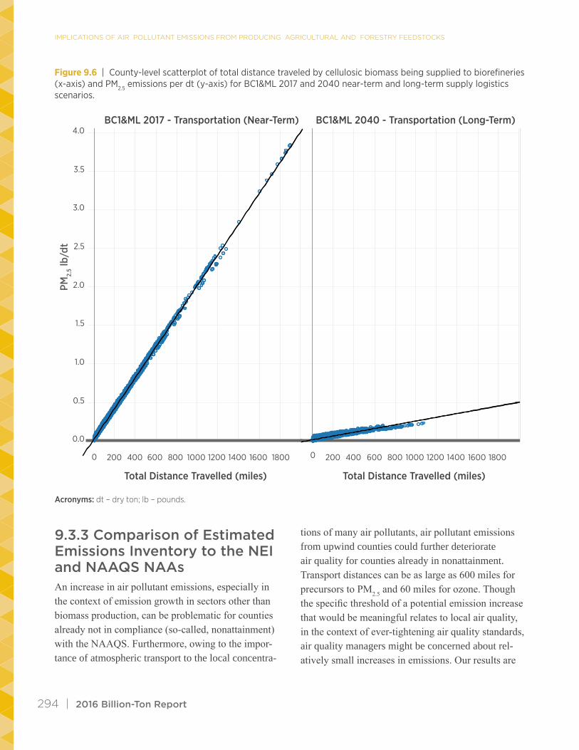
Figure 9.6 shows county-level scatter plots of total distance traveled by stover to supply biorefineries and the emissions that would be generated per unit of biomass for transporting that biomass. As distance increases, emissions generally increase, as indicated by trends in figure 9.6. This figure also indicates that relative to the near-term system, the long-term feed-stock supply logistics system reduces emissions for the same distance traveled through biomass densifi-cation. A regression line was fit to the data in figure 9.6. The regression shows a good fit (R-squared = 98%) for the near-term logistics system and a less good fit (R-squared = 78%) for the long-term sys-tem. Increased variability in the long-term logistics system reflects reduced emissions from fuel use and increased importance of more variable fugitive dust emissions. Fugitive dust emissions are highly vari-able due to the variability in assumptions about local conditions (e.g., climate, on-road traffic, silt loading) for fugitive dust estimates.

2016 Billion-Ton Report | 293
Non
-Har
vest
Har
vest
On-
Road
Tr
ansp
ort
Chem
ical
App
licat
ion
Prep
roce
ssin
g
0%
50%
100%
0%
50%
100%
0%
50%
100%
Non
-Har
vest
Har
vest
On-
Road
Tr
ansp
ort
0%
50%
100%
0%
50%
100%
0%
50%
100%
0%
50%
100%
0%
50%
100%
PM2.5
NOxVOCNH3
SR SG MS LR TB SR SG MS LR TB
SR SG MS LR TB
SR SG MS LR TB
SR SG MS LR TB
PM10
SR SG MS LR TB
CO
SR SG MS LR TB
SOx
SR SG MS LR TB(n) 2101,5471,4071,034574
Figure 9.5 | Distribution of county-level estimates (number of counties = n) of the fraction of aggregated mass emissions from five categories of emitting activities. Estimates are for potential biomass produced and supplied9 for the BC1&ML 2040 scenario. Blanks indicate no emissions from that activity category for that feedstock and pollutant. Box and whisker plots represent minimum, 25th percentile, median, 75th percentile, and maximum.
9 Only a subset of biomass produced is being supplied to biorefineries in the scenarios examined as a part of BT16 and therefore, in a given county, potential biomass produced may not be used for biofuel production (DOE 2016). For example, wheat straw and corn grain are not supplied to biorefineries.
Acronyms: CO – carbon monoxide; NH3 – ammonia; NOx – oxides of nitrogen; PM – particulate matter; SOx – oxides of sulfur; VOC – volatile organic com-pounds; CG – corn grain; LR – logging; MS – miscanthus; SG – switchgrass; SR – stover; SW – straw; TB – whole-tree biomass.
ImPlIcAtIons oF AIr PollutAnt EmIssIons From ProducIng AgrIculturAl And ForEstry FEEdstocks
294 | 2016 Billion-Ton Report
Figure 9.6 | County-level scatterplot of total distance traveled by cellulosic biomass being supplied to biorefineries (x-axis) and PM2.5 emissions per dt (y-axis) for BC1&ML 2017 and 2040 near-term and long-term supply logistics scenarios.
BC1&ML 2017 - Transportation (Near-Term) BC1&ML 2040 - Transportation (Long-Term)
0 200 400 600 800 1000 1200 1400 1600 1800
Total Distance Travelled (miles)
0 200 400 600 800 1000 1200 1400 1600 1800
Total Distance Travelled (miles)
0.0
0.5
1.0
1.5
2.0
2.5
3.0
3.5
4.0
PM2.
5 lb/
dt
Acronyms: dt – dry ton; lb – pounds.
9.3.3 Comparison of Estimated Emissions Inventory to the NEI and NAAQS NAAs An increase in air pollutant emissions, especially in the context of emission growth in sectors other than biomass production, can be problematic for counties already not in compliance (so-called, nonattainment) with the NAAQS. Furthermore, owing to the impor-tance of atmospheric transport to the local concentra-
tions of many air pollutants, air pollutant emissions from upwind counties could further deteriorate air quality for counties already in nonattainment. Transport distances can be as large as 600 miles for precursors to PM2.5 and 60 miles for ozone. Though the specific threshold of a potential emission increase that would be meaningful relates to local air quality, in the context of ever-tightening air quality standards, air quality managers might be concerned about rel-atively small increases in emissions. Our results are

2016 Billion-Ton Report | 295
reported in a way that is intended to help inform air quality managers about air emissions from poten-tial biomass production that could be translated into locally relevant decision factors.
The first panels in figures 9.7–9.9 display distribu-tions of the emission ratios comparing the inventory to the 2011 NEI for each NAAQS criteria air pollut-ant based on mass air pollutant emissions estimated for the BT16 scenarios. Results are presented for pre-cursors to ozone, PM2.5, and PM10 (table 9.3), as well as for SO2, NO2, and CO emissions. Distributions are shown for counties in attainment or nonattainment with the NAAQS. Any increase in emissions has the potential to contribute to air quality degradation in or upwind of a county, but of particular interest are those counties whose emission ratios are potentially greater than a threshold (Zhang et al. 2016). An emis-sion ratio above 1% is suggested as a threshold that any county might consider as potentially significant. An emission ratio greater than 1% does not indi-cate that air quality degradation will occur, but that emissions in those counties warrant further analysis by air quality managers in the context of a reference scenario to determine the potential for air quality degradation in or upwind of that county. Counties in nonattainment whose emission ratios are above the suggested threshold of 1% are considered among the most at-risk for potential air quality degradation.
The maps in figures 9.7–9.9 display the emission ratios for each NAAQS criteria air pollutant along with locations of NAAs for these pollutants as of 2015 (EPA 2016d). NAAs are designated based on the currently enforced primary standards 10 for ozone (8-hour standard), PM2.5 (24-hour and 1-year), PM10 (24-hour), SO2 (1-hour), NO2 (1-hour and 1-year), and CO (8-hour and 1-hour) NAAQS. Increases in emissions even in counties in attainment for NAAQS could impact NAAs downwind, owing to atmospher-ic transport.
This chapter focuses discussion on emission ratios for ozone, PM2.5, and PM10 in the context of counties in NAAs. No county is out of compliance with the current NO2 and CO NAAQS (EPA 2016b). SO2 is not transported upwind, so we only discuss emission ratios for SO2 in NAAs. For additional results for SO2, NO2, and CO, please refer to appendix 9-A, section 9A.3.1.
9.3.3.1 Counties Upwind from NAAs
Figures 9.7–9.9 show that in the BC1&ML 2017 and 2040 scenarios, about 25% of the total number of counties evaluated (~3,000) in attainment with the NAAQS for ozone, PM2.5 and PM10 have emis-sion ratios greater than 1% for each pollutant. In the BC1&ML scenarios, the upper quartile of county-lev-el emission ratios for ozone range from 0.8% to 10% in 2017 and 0.7% to 8% in 2040. In the BC1&ML scenarios, the upper quartile of county-level emis-sion ratios for PM2.5 range from 0.9% to 10% in 2017 and 2% to 10% in 2040 with many counties having emission ratios above 1% in both years. In the BC1&ML scenarios, the upper quartile of county-lev-el emission ratios for PM10 range from 0.9% to 8% in 2017 and 2% to 11% in 2040. We visually display all counties with emission ratios alongside those counties currently in nonattainment with applicable NAAQS because air quality in any location could be affected by emissions upwind.
Figure 9.7 shows areas in nonattainment with ozone NAAQS that are upwind (on the order of 60 miles) of multiple counties with ozone precursor emission ratios greater than 1% in BC1&ML 2017 and 2040 scenarios. In 2017, these areas include the city of Chicago, Illinois (eleven counties); Cincinnati, Ohio (nine counties); and Columbus, Ohio (six counties). In 2040, areas with nonattainment counties adjacent to multiple attainment counties with emission ratios greater than 1% include the city of Chicago, Illinois
10 There are also secondary standards intended to provide public welfare protection against decreased visibility and damage to animals, crops, vegetation, and buildings rather than health. These secondary standards are not considered in our analysis.

ImPlIcAtIons oF AIr PollutAnt EmIssIons From ProducIng AgrIculturAl And ForEstry FEEdstocks
296 | 2016 Billion-Ton Report
(eleven counties); St. Louis, Missouri (eight coun-ties); and Memphis, Arkansas (three counties). The majority of these counties have potential agricultural residue production in 2017 and 2040 scenarios and energy crop production in the 2040 scenario. As a re-sult, the emission ratios above 1% are largely attrib-utable to NOX and VOC emissions from fertilizer and pesticide application as well as NOX emissions from transportation.
Figures 9.8 and 9.9 show areas in nonattainment with PM2.5 and PM10 NAAQS that are upwind (on the order of 600 miles) of multiple counties with PM2.5 and PM10 precursor emission ratios greater than 1% in BC1&ML 2017 and 2040 scenarios. For PM2.5 es-timated for the 2017 scenario, these upwind counties are located around the city of Louisville, Kentucky (four counties); Lane and Klameth Counties, Oregon; Lincoln County, Montana; and Shoshone County, Idaho. For PM2.5 in 2040 these upwind counties are located around the city of St. Louis, Missouri (eight counties); the city of Louisville, Kentucky (four counties); the city of Cleveland, Ohio (two counties); and Lincoln County, Montana. For PM10 estimated in 2017, the upwind county is Lane County, Oregon. For PM10 in 2040, upwind counties include Shoshone County, Idaho, and five counties in northwest Mon-tana. The high PM2.5 and PM10 emission ratios in these areas are largely attributable to three sources: (1) the application of fertilizers and pesticides, which contribute to changes in PM precursor emissions (NH3, NOX, and VOC); (2) fugitive dust emissions from the use of agricultural equipment, which contribute to PM2.5; and (3) NOX and SOX emissions from transportation of any biomass, which are PM precursor emissions (table 9.3).
If future biomass production sources of air pollutants are additional and do not displace current biomass production sources (see section 9.4), air pollutant emissions from these sources may pose challenges for compliance with the NAAQS in these select-ed areas. The emission estimates provided in this study could help inform long-term air quality plan-
ning, such as state implementation plans, which are required to consider new emission sources for future scenarios.
9.3.3.2 Counties in NAAs
Figure 9.7 shows how the locations of counties in nonattainment for ozone with emission ratios great-er than 1% for ozone precursors differ by year for the BC1&ML 2017 and 2040 and HH3&HH 2040 scenarios. For the BC1&ML 2017 scenario, the nonattainment counties with emission ratios esti-mated to be greater than 1% are Kings and Tulane counties in California, Madison and Knox counties in Ohio, and Kane County in Illinois. The emissions in 2017 would be primarily concentrated in coun-ties with agricultural residue production, with the exception being Knox County, Ohio, where forestry biomass would be a major contributor to ozone pre-cursor emissions (VOC and NOX). However, for the BC1&ML 2040 scenario, the non-attainment coun-ties with ozone precursor emission ratios greater than 1% have shifted to St. Claire and Monroe counties, Illinois; and Crittenden County, Arkansas. In the HH3&HH 2040 scenario, the additional counties in NAA estimated to have ozone emission ratios greater than 1% are Grundy and Kendall counties in Illinois; and Madison, Clinton, Fairfield, and Knox counties, Ohio; Crittenden County, Arkansas; and Hamilton County, Texas.
Similarly, figure 9.8 shows how the locations of counties in NAAs for PM2.5 with emission ratios greater than 1% for PM2.5 vary by year for the BC1&ML scenarios. In 2017, these areas are in Kings, Tulare, and Merced counties, California; Lin-coln County, Montana; and Shoshone County, Idaho. However, in the BC1&ML 2040 scenario, non-attain-ment counties with PM2.5 emission ratios higher than 1% are Monroe, St. Claire, and Randolph counties in Illinois, as well as Franklin County in Missouri. In the HH3&HH 2040 scenario, no additional counties in NAAs are estimated to have PM2.5 emission ratios greater than 1%.
2016 Billion-Ton Report | 297
Shifts in both ozone precursors as well as primary and secondary PM2.5 emissions from 2017 to 2040 scenarios are due to a combination of several factors. In 2040, decreased whole-tree biomass production (e.g., Knox and Lincoln counties), higher agricultural residue yields (e.g., Kings, Monroe, and St. Claire counties), and decreases in the average distance of biomass on-road transportation using the long-term logistics system (most counties) would reduce the ozone and PM2.5 emission ratios in non-attainment counties with ratios greater than 1% in 2017 to less than 1% in 2040. Increased potential energy crop production in combination with continuing agricul-tural residue production, in the nonattainment coun-ties in 2040 would lead to ozone and PM2.5 precursor emission ratios greater than 1% in a different set of counties relative to 2017. Additional differences in emission ratios between the BC1&ML 2040 and the HH3&HH 2040 scenario are due to additional transportation to biorefineries of potential additional biomass produced.
Figure 9.9 shows how the locations of counties in NAAs for PM10 with emission ratios greater than 1% for PM10 vary by year for the BC1&ML and HH3&HH scenarios. In 2017, these areas are in Lin-coln County, Montana, and Shoshone County, Idaho. However, in the BC1&ML 2040 scenario, Flathead County, Montana, is the only nonattainment county with a PM10 with an emission ratio higher than 1% and Flathead County, Montana, and Power County, Idaho are nonattainment counties with a PM10 emis-sion ratios higher than 1% in the HH3&HH scenari-os. Changes in the emission ratio across these scenar-ios reflect decreased forestry biomass use for energy (e.g., in Montana and Idaho) and increased fugitive dust from agricultural residues, in particular straw, in Power County, Idaho.
The emissions that would be generated in counties with emission ratios greater than 1% for ozone and PM10 can generally be attributed to a few primary sources. Emissions from counties with high quanti-
ties of agricultural-residue production and emission ratios greater than 1% for ozone would be largely attributable to NOX and VOC emissions from chem-ical application and on-road biomass transportation. Greater than 1% PM10 emission ratios would be attributable mostly to fertilizer and pesticide applica-tions, contributing to PM precursor emissions (NH3, NOX, and VOC), fugitive dust emissions from the use of agricultural equipment that contribute to PM10, as well as NOX and SOX emissions from biomass on-road transportation. In addition, emissions from whole-tree biomass are largely attributable to on-road biomass transportation.
The results for emission ratios in NAAs for SO2 differ from those for ozone and PM. For SO2, only partial counties are in NAAs, so local air quality and transportation modeling would be needed to understand biomass transportation through NAAs in the county. For the BC1&ML 2017 scenario, only Muscatine County, Iowa, has an emission ratio that is greater than 1% for SO2. For the BC1&ML 2040 sce-nario, in Muscatine County, Iowa, and Pike County, Indiana, emission ratios are greater than 1%. In the 2040 HH3&HH scenario, Muscatine County, Iowa; Pike County, Indiana; and Tazewell, Illinois, the NEI ratio is greater than 1%. The emission ratios in Muscantine, Pike, and Tazewell counties are large-ly attributable to transporting stover (i.e., up to 20 miles) and miscanthus to surrounding counties (i.e., up to 80 miles), respectively.

ImPlIcAtIons oF AIr PollutAnt EmIssIons From ProducIng AgrIculturAl And ForEstry FEEdstocks
298 | 2016 Billion-Ton Report
Figure 9.7 | BC1&ML 2017 and 2040 scenarios’ county-level distributions of emission ratios for ozone in BC1&ML 2017 and 2040 scenarios (top frame).11 Maps of emission ratios and non-attainment counties at the end of 2015 ex-ceeding NAAQS standards for ozone (primary, 8-hour) (EPA 2016d)12 are displayed in red in the 2017 (middle frame) and 2040 (bottom frame) maps. Box and whisker plots represent minimum, 25th percentile, median, 75th percen-tile, and maximum. BC1&ML
2017 2040
Counties in Attainment
Whole or Partial Counties in Non-Attainment
Whole or Partial Counties in Non-Attainment
Counties inAttainment
Emis
sion
Rat
io -
Ozo
ne P
recu
rsor
Em
issi
ons
0.000001%
0.000010%
0.000100%
0.001000%
0.010000%
0.100000%
1.000000%
10.000000%
100.000000%
11 See text for a complete list of nonattainment counties with emission ratios above 1%.12 Includes NAA designations for the 2008 NAAQS that are still in force.

2016 Billion-Ton Report | 299

ImPlIcAtIons oF AIr PollutAnt EmIssIons From ProducIng AgrIculturAl And ForEstry FEEdstocks
300 | 2016 Billion-Ton Report
Figure 9.8 | BC1&ML 2017 and 2040 scenarios’ county-level distributions of emission ratios for PM2.5 (top frame).13 Maps of emission ratios and non-attainment counties at the end of 2015 exceeding NAAQS standards for PM2.5 (pri-mary, 24-hour and 1-year) (EPA 2016d)14 are displayed in red in the 2017 (middle frame) and 2040 (bottom frame) maps. Box and whisker plots represent minimum, 25th percentile, median, 75th percentile, and maximum.
BC1&ML
2017 2040
Counties in Attainment
Whole or Partial Counties in Non-Attainment
Whole or Partial Counties in Non-Attainment
Counties inAttainment
0.000001%
0.000010%
0.000100%
0.001000%
0.010000%
0.100000%
1.000000%
10.000000%
100.000000%
Emis
sion
Rat
io -
PM
2.5 P
recu
rsor
Em
issi
ons
13 See text for a complete list of nonattainment counties with emission ratios above 1%.14 Includes NAA designations for the 1997, 2006, and 2012 NAAQS that are still in force.

2016 Billion-Ton Report | 301

ImPlIcAtIons oF AIr PollutAnt EmIssIons From ProducIng AgrIculturAl And ForEstry FEEdstocks
302 | 2016 Billion-Ton Report
Figure 9.9 | BC1&ML 2017 and 2040 scenarios’ county-level distributions of emission ratios for PM10 (top frame).15 Maps of emission ratios and non-attainment counties at the end of 2015 exceeding NAAQS standards for PM10 (pri-mary, 24-hour) (EPA 2016d)16 are displayed in red in the 2017 (middle frame) and 2040 (bottom frame) maps. Box and whisker plots represent minimum, 25th percentile, median, 75th percentile, and maximum.
BC1&ML
2017 2040
Counties in Attainment
Whole or Partial Counties in Non-Attainment
Whole or Partial Counties in Non-Attainment
Counties inAttainment
0.000001%
0.000010%
0.000100%
0.001000%
0.010000%
0.100000%
1.000000%
10.000000%
100.000000%
Emis
sion
Rat
io -
PM
10 P
recu
rsor
Em
issi
ons
15 See text for a complete list of nonattainment counties with emission ratios above 1%.16 Includes NAA designations for the 1987 and 2012 NAAQS that are still in force.

2016 Billion-Ton Report | 303

ImPlIcAtIons oF AIr PollutAnt EmIssIons From ProducIng AgrIculturAl And ForEstry FEEdstocks
304 | 2016 Billion-Ton Report
9.3.4 Additional DiscussionIn addition to comparing estimated emissions from the BT16 scenarios to emissions in the NEI, we qualitatively discuss significant upstream emissions associated with potential biomass feedstock produc-tion and briefly discuss emissions from biomass and petroleum fuel production.
9.3.4.1 Life-Cycle Assessments
Zhang et al. (2016) compared the Greenhouse Gases, Regulated Emissions, and Energy Use in Transporta-tion (GREET) Model’s (ANL 2015) national aver-age life-cycle air pollutant emissions to FPEAM’s spatially explicit inventory of emissions for biomass feedstocks. Direct comparisons are limited by the systems boundary of GREET, which also quantifies upstream emissions, and FPEAM, which estimates only direct local emissions. In addition, GREET does not include fugitive dust emissions, NH3 emissions, or VOC emissions from pesticides or biomass prepro-cessing and drying. Fleet age and turnover, as well as other assumptions about equipment in the MOVES/NONROAD models that are used by FPEAM, also differ from GREET assumptions.
To identify potentially significant sources of upstream emissions, which could motivate future analysis, we qualitatively compared the results of our analysis of direct, anthropogenic emissions from feedstock pro-duction and logistics to life-cycle criteria air pollutant emissions from GREET. We reviewed GREET for activities that emit air pollutant emissions per unit of biomass of a similar or larger magnitude as direct emissions sources analyzed in this chapter.
Based on the GREET model (ANL 2015), three potentially large sources of upstream emissions should be modeled in a spatially explicit fashion on a county-level basis (ANL 2015). GREET estimated that fertilizer manufacturing (primarily N-based) and transportation-related emissions are about as high as our estimated emissions from direct use of the fertilizer (ANL 2015). Other potentially large
sources of upstream emissions are agricultural and forestry equipment manufacturing and maintenance (ANL 2015). This topic requires further research as GREET’s equipment modeling only includes the capability to model one equipment type for biomass feedstocks, and the amortization of those emissions over the life of the equipment are not well aligned with our analysis (i.e., MOVES 2014a assumptions).
9.3.4.2 Crude Oil
Because biofuel is considered an alternative to petroleum-based gasoline and diesel fuels, anoth-er potential point of comparison is crude oil. The GREET model estimates that life-cycle air pollutant emissions from crude oil production and transport are lower than from biomass feedstocks (ANL 2015). A detailed comparison between GREET and FPEAM is not made because of the differences in system boundaries noted above. An inventory assessment of crude oil is a potential alternative that we can com-pare our assessment to. Existing assessments, such as one by Tessum, Hill, and Marshall (2014), also indicate that crude oil production generally emits fewer air pollutant emissions than biomass feedstocks on the basis of miles traveled using the fuel. How-ever, studies (e.g., Tessum, Marshall, and Hill 2012) have shown that biofuels could have lower life-cycle criteria air pollutant emissions than their counterpart petroleum-based fuels. This is primarily attributable to the benefits of coproducts considered in life-cycle assessments (LCAs), such as electricity produced from the biofuel conversion process, displacing prod-ucts derived from fossil fuels.
A detailed and specific analysis of crude oil is beyond the scope of this chapter. A more constrained in-ventory assessment of crude oil produced, supplied, and used in the United States would be feasible, but it would be misleading to compare that to biomass without taking a life-cycle approach because the emission sources in the biofuel life-cycle differ sig-nificantly from those in the petroleum fuel life-cycle. In addition, in order to understand “net” impacts of

2016 Billion-Ton Report | 305
biofuel compared to petroleum, an integrated analysis would be needed to estimate when, where, and how much fuel might be displaced. Although a limited emissions inventory of only crude oil and the associ-ated integrated analysis would not allow for a com-plete comparison between biomass and crude oil, it would help identify counties where air quality could improve because of reduced production of domestic crude oil and transportation of that oil. One benefit of biomass production for biofuels is that emissions from feedstock production and transportation, as well as emissions from biorefineries, are likely located in rural counties. U.S. petroleum refineries are large-ly located in or near urban areas, and therefore the exposure of populations and resulting health effects could change, depending on the fuel’s supply chain. Consequently, there could be a complex and new pattern of air quality considerations when consider-ing net emissions from a high biofuels penetration scenario.
9.3.4.3 Preprocessing Emissions Resulting from Electricity Usage
To test the significance of excluding upstream emis-sions from the BT16 air pollutant emissions inventory, we performed a sensitivity analysis to estimate emis-sion rates resulting from the electricity use of biomass preprocessing equipment. Other than the on-site wood chipper for processing whole-tree biomass, preprocess-ing equipment exclusively uses electricity. It is import-ant to note that emissions from the generation of the electricity used in the preprocessing would, in general, not be emitted near the point of use. In addition, because the source of generated electrons is not known, we cannot specifically pinpoint the location of the upstream electricity generation emissions.
Table 9.5 summarizes air pollutant emission rates from electricity used with preprocessing equipment, assum-ing a U.S. grid mix; regional grid mixes are further discussed in the appendix section 9A.2.3. Emission estimates are based on the sum of preprocessing equip-
ment electricity use from equipment budgets used in BT16 volume 1 and the methodology documented in appendix section 9A.2.3. The long-term supply logistics system uses more than four times as much electricity as the near-term system. Thus, upstream emissions from electricity generated to supply power to preprocessing equipment used in 2040 would be far higher than those associated with 2017 feedstock preprocessing. How-ever, while electricity consumption is much higher for long-term logistics systems than near-term ones, the net effects across the life cycle could ameliorate or neutral-ize any effect on increased air emissions because air emissions at the biorefinery should decrease owing to reduced preprocessing requirements (at the biorefinery) and more efficient conversion of feedstocks to fuels, etc.
Comparing table 9.5 to figures 9.2 and 9.3 indicates that the use of electricity in preprocessing equipment leads to large, non-local SOX emissions because of a higher share of electricity generated from oil and coal compared to natural gas or renewable energy sources (see EFs in table 9A.6). If coal or oil plants are located in or near NAAs, it is possible that these areas will face increased challenges to comply with SO2 NAAQS. However, with decreased use of coal and oil for electricity generation by 2040 (EIA 2016), upstream CO and SOX emissions associated with electricity generation would be expected to decrease. If preprocessing is occurring on the site of cellulos-ic biorefineries, lignin could be burned to produce electricity. The use of lignin for electricity would have tradeoffs in local emissions (e.g., NOX, PM, GHGs, SO2) at the biorefinery, as compared to non-local emissions from electricity generation at power plants. Upstream NOX emissions from the use of electricity in preprocessing equipment in long-term systems would be relatively low, but the emissions are higher than emissions from whole-tree biomass production due to the lack of chemical application for most whole-tree biomass. Finally, upstream VOC, PM10, and PM2.5 emissions from electricity generation would be lower than those from biomass production in the lowest emitting county.17
17 This excludes forestry residues and biomass due to the lack of quantification of fugitive dust emissions.
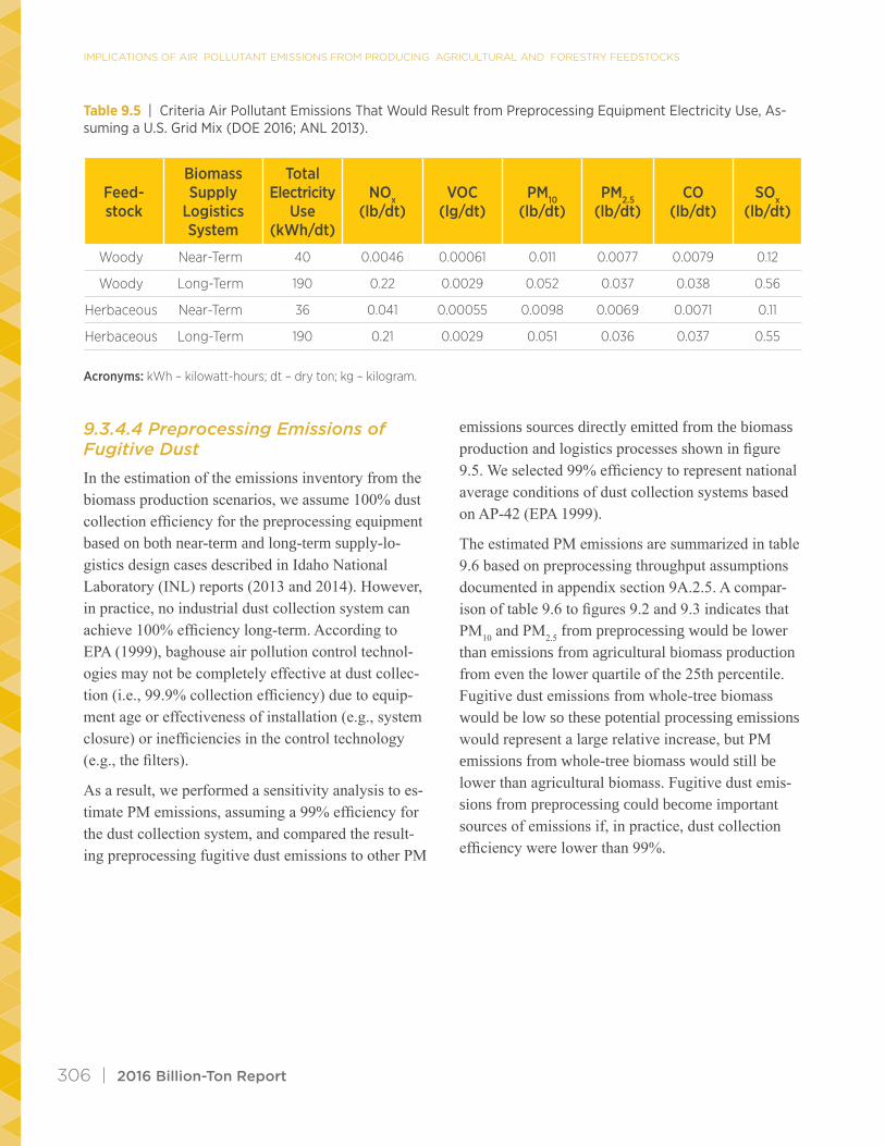
ImPlIcAtIons oF AIr PollutAnt EmIssIons From ProducIng AgrIculturAl And ForEstry FEEdstocks
306 | 2016 Billion-Ton Report
Table 9.5 | Criteria Air Pollutant Emissions That Would Result from Preprocessing Equipment Electricity Use, As-suming a U.S. Grid Mix (DOE 2016; ANL 2013).
Feed-stock
Biomass Supply
Logistics System
Total Electricity
Use (kWh/dt)
NOx (lb/dt)
VOC (lg/dt)
PM10 (lb/dt)
PM2.5 (lb/dt)
CO (lb/dt)
SOx (lb/dt)
Woody Near-Term 40 0.0046 0.00061 0.011 0.0077 0.0079 0.12
Woody Long-Term 190 0.22 0.0029 0.052 0.037 0.038 0.56
Herbaceous Near-Term 36 0.041 0.00055 0.0098 0.0069 0.0071 0.11
Herbaceous Long-Term 190 0.21 0.0029 0.051 0.036 0.037 0.55
Acronyms: kWh – kilowatt-hours; dt – dry ton; kg – kilogram.
9.3.4.4 Preprocessing Emissions of Fugitive Dust
In the estimation of the emissions inventory from the biomass production scenarios, we assume 100% dust collection efficiency for the preprocessing equipment based on both near-term and long-term supply-lo-gistics design cases described in Idaho National Laboratory (INL) reports (2013 and 2014). However, in practice, no industrial dust collection system can achieve 100% efficiency long-term. According to EPA (1999), baghouse air pollution control technol-ogies may not be completely effective at dust collec-tion (i.e., 99.9% collection efficiency) due to equip-ment age or effectiveness of installation (e.g., system closure) or inefficiencies in the control technology (e.g., the filters).
As a result, we performed a sensitivity analysis to es-timate PM emissions, assuming a 99% efficiency for the dust collection system, and compared the result-ing preprocessing fugitive dust emissions to other PM
emissions sources directly emitted from the biomass production and logistics processes shown in figure 9.5. We selected 99% efficiency to represent national average conditions of dust collection systems based on AP-42 (EPA 1999).
The estimated PM emissions are summarized in table 9.6 based on preprocessing throughput assumptions documented in appendix section 9A.2.5. A compar-ison of table 9.6 to figures 9.2 and 9.3 indicates that PM10 and PM2.5 from preprocessing would be lower than emissions from agricultural biomass production from even the lower quartile of the 25th percentile. Fugitive dust emissions from whole-tree biomass would be low so these potential processing emissions would represent a large relative increase, but PM emissions from whole-tree biomass would still be lower than agricultural biomass. Fugitive dust emis-sions from preprocessing could become important sources of emissions if, in practice, dust collection efficiency were lower than 99%.

2016 Billion-Ton Report | 307
Table 9.6 | PM10 and PM2.5 Emissions from Preprocessing Equipment, Assuming a 99% Efficiency of the Dust Collec-tion System (DOE 2016; Krause and Smith 2006; WLA Consulting 2011; Davis et al. 2013)
FeedstockBiomass Supply Logistics System
Preprocessing Throughput
(dt/hr)
PM10 (lb/dt)
PM2.5 (lb/dt)
Woody Near-Term 8.5a 0.21 0.035
Woody Long-Term 8.5a 0.21 0.035
Herbaceous Near-Term 5 0.35 0.059
Herbaceous Long-Term 6.5 0.27 0.046
a Two processing steps with a maximum throughput of 17 dt per 2 hours from SCM budget data (DOE 2016).
Acronyms: dt – dry ton; lb – pounds.
9.4 DiscussionThe objectives of this analysis are (1) to estimate the air pollutant emissions for selected biomass produc-tion, harvest, transportation, and preprocessing sce-narios; (2) to determine spatially where these emis-sions would occur and how these emissions could potentially impact air quality; and (3) to identify potential opportunities to minimize potential adverse impacts.
9.4.1 Implication of ResultsFuture air pollutant emissions resulting from large-scale deployment of production and supply logistics as depicted in the BT16 scenarios, if realized and additional (rather than displacing other agriculture or forestry activities), could yield increases in emissions that could pose challenges for areas to attain the NAAQS. The implications of air emission estimates presented in this chapter are discussed in this section in regard to feedstock comparison, potential areas where emissions might increase, sources of emis-sions, and opportunities for emission mitigation.
9.4.1.1 Feedstock Comparison
For biomass production on a per-unit-of-biomass ba-sis, agricultural residues are likely to lead to lower air
pollutant emissions than agricultural crops because of tillage and field establishment activities (other than fertilizer application) not being allocated to the residues. However, because harvest and collection of agricultural residues are additional activities beyond those required for growing and harvesting grains, the emissions from these “extra” activities are more likely than energy crops to represent additional emis-sions. The production of residues requires that the primary crop be grown.
While switchgrass and miscanthus have higher emissions than agricultural residues, the production of these two energy crops is estimated to generate lower emissions than corn grain (the most commonly used feedstock for biofuel at present) on a per-unit of biomass basis due to their greater yield. Relative to agricultural residues, growing energy crops may replace corn grain and other conventional crops, and therefore the “net” change in air emissions will be much smaller than the emissions resulting from growing and harvesting the energy crops. In fact, if switchgrass and miscanthus replace annual crops, it is possible that this displacement would lead to reduc-tions in air emissions.
For biomass production, logging residues and whole-tree biomass are estimated to produce NH3, NOX, and VOC emissions that are similar to or lower than agri-

ImPlIcAtIons oF AIr PollutAnt EmIssIons From ProducIng AgrIculturAl And ForEstry FEEdstocks
308 | 2016 Billion-Ton Report
cultural biomass feedstocks (on a per-unit-of-biomass basis) because of overall lower chemical application. Total PM emissions from logging residues and trees are not comparable to those for other feedstocks because the fugitive dust emissions from whole-tree biomass are not quantified. However, equipment use leads to CO and SOX emissions from whole-tree bio-mass that are similar per dt to agricultural feedstocks (with logging residues leading to fewer emissions owing to the allocation assumptions). Since BT16 volume 1 assumes that the land base for forestry does not change in BT16 scenarios, the equipment for whole-tree biomass is the same as that for conven-tional forestry, so changes from conventional uses to energy uses are less likely to change emissions from the production of whole-tree biomass.
On a per-unit-of-biomass basis, on-road transporta-tion is a major source of NOX, CO, and SOX emis-sions, so the differences between various cellulosic feedstocks for a pollutant would shrink because emissions vary by transportation distance rather than feedstock type. The most noticeable remaining dif-ference between emissions from different cellulosic feedstocks is that NOX, CO, and SOX off-site trans-portation emissions from logging residues are higher than emissions from other biomass feedstocks. Low logging residue production costs allow for longer dis-tances (i.e., increased transportation costs) and still fall within the $100 per dt cutoff for the supply lo-gistics scenario. Relative to biomass production only, NH3, PM2.5, and PM10 emitted per unit of biomass by each feedstock remains similar across feedstocks when accounting for on-road transportation and pre-processing. Relative to biomass production, whole-tree biomass NH3, PM2.5, and PM10 emissions would increase because of the limited chemical application and the lack of fugitive dust emission estimates for whole-tree biomass production in this analysis.
9.4.1.2 Potential Areas Where Emissions Might Occur
This analysis identifies counties in attainment with NAAQS for ozone, PM2.5, and PM10 that are estimat-ed to have emission ratios greater than 1%. About 25% of the counties evaluated for ozone, PM2.5, and PM10 would have emission ratios above 1% with emission ratios reaching about 10% and 11% in BC1&ML 2017 and 2040 scenarios, respectively. An emissions ratio above 1% is suggested as a threshold that any county might consider a potentially signifi-cant increase in emissions that would warrant further attention by air quality managers in anticipating po-tential air quality degradation or degradation upwind of that county. Counties in nonattainment whose emission ratios are above the suggested threshold of 1% are considered among the most at risk for sub-stantial air quality degradation.
Another important consideration for contextualizing the results of this analysis is that long transport dis-tances could result in precursor pollutants being emit-ted upwind of counties without significant cellulosic feedstock production. These transportation emissions could impact the emissions in upwind counties. For instance, the emissions from many Midwest and Corn Belt counties, despite largely being in compliance with the NAAQSs, could contribute to concentrations of PM2.5 or ozone in other states downwind. The emissions inventory developed here can be further utilized for air quality modeling by creating temporal profiles and chemical speciation for each emission source. This would help determine the air quality and human health impacts of potential biomass feedstock production. Alternatively, the emissions inventory can be coupled with an air quality screening tool such as EPA’s Co-Benefits Risk Assessment (COBRA) screening model to evaluate important changes in emission concentrations and potential changes in human health (EPA 2015b).18
18 Other potential screening tools include InMAP (Intervention Model for Air Pollution) (Tessum et al. 2016), APEEP/AP2 (Air Pollu-tion Emission Experiments and Policy analysis model) (Muller and Mendelsohn 2011), and EASIUR (Estimating Air pollution Social Impact Using Regression) (Heo and Adams 2016).

2016 Billion-Ton Report | 309
The estimated air pollutant emissions inventory indi-cates that the potential changes in ozone and PM2.5 precursor emissions (i.e., 2011 NEI ratio) from BT16 cellulosic biomass production and supply in nonat-tainment counties are greater than 1% of the NEI in a few counties. Specifically in the BC1&ML 2017 scenario, there are nine counties in nonattainment for ozone, PM2.5, PM10, or SO2 NAAQSs located in California, Ohio, Illinois, Iowa, Montana, and Idaho. Also in the BC1&ML 2040 scenario, there are eight counties in nonattainment for ozone, PM2.5, or SO2 NAAQSs located in Arkansas, Iowa, Illinois, Mis-souri, Indiana, and Montana. In the HH3&HH 2040 scenario, there are 17 counties in nonattainment for ozone, PM2.5, or SO2 NAAQSs located in Arkansas, Illinois, Missouri, Ohio, Iowa, Indiana, Texas, Mon-tana, and Idaho. Emission ratios in these counties that are greater than 1% of NEI emissions indicate that there could be increased challenges for these counties to meet NAAQS under the scenarios. When comparing the 2017 scenario to the 2040 scenario, counties that may experience a greater increase in air emissions would shift geographically because of the change in county-wide biomass production (such as the type and quantity of biomass feedstocks produced).
9.4.1.3 Sources of Emissions and Opportunities for Emission Mitigation
The results of the inventory indicate several potential improvements that could mitigate risks to NAAs. The emissions estimated here for cellulosic biomass feedstocks could be further mitigated through the application of several emission reduction strategies. A comparison of the BC1&ML 2040 and HH3&HH 2040 scenarios indicates that much more biomass could be produced with only a marginal increase of about 1%–2% in emission ratios nationwide.
The use of more efficient equipment or equipment that requires fewer passes in NAAs could reduce the risk of changing local air quality by decreasing emis-
sions per acre planted or harvested, as well as per unit of biomass produced or supplied. This is important as potential equipment improvement from 2017 to 2040 is not captured in BT16. For example, this analysis il-lustrates that the long-term feedstock supply logistics system itself could also reduce emissions per mile traveled through feedstock densification. In addition, using biomass more locally or using more fuel-effi-cient long-distance transportation methods (e.g., rail) could potentially decrease emissions from long-dis-tance truck transport.
The use of less-intensive tillage practices for conven-tional agricultural crops such as corn grain would, in part, offset additional emissions from the harvest, collection, and transport of agricultural residues in NAAs. Furthermore, while the use of waste biomass (e.g., yard wastes and construction and demolition wastes) was not examined in this chapter, its use could also lower estimated emissions based on its lack of chemical application, tillage, and harvest activities.
Finally, constraining biomass grown or the types of biomass grown or collected (e.g., crop residues) in counties in NAAs or geographically near counties at risk for being in nonattainment is another potential mitigation strategy for potential future biomass pro-duction and supply. For example, agricultural residues are more likely to lead to emissions that are in addition to emissions from corn grain cultivation than energy crops that might replace conventional crops. Anoth-er option is that for some pollutants, such as PM, an option to prevent emissions moving upwind could be establishing buffer vegetation near agricultural lands. For example, research has shown that vegetation in forested areas can potentially remove 80%–100% of particulate emissions (Pace 2005).
9.4.2 Limitations of This StudyBT16 volume 1 estimates potential biomass pro-duction in the future. There is inherent uncertainty associated with evaluating feedstocks not currently
ImPlIcAtIons oF AIr PollutAnt EmIssIons From ProducIng AgrIculturAl And ForEstry FEEdstocks
310 | 2016 Billion-Ton Report
produced at a commercial scale. As a result, the estimates of potential improvements to current crops and the comparative analysis across feedstocks could also change in the future. While our modeling of the practices and inputs for cellulosic feedstock produc-tion uses the best available information, the lack of long-term, commercial-scale production of cellulosic feedstocks (especially dedicated energy crops like switchgrass) leads to uncertainty in our results.
In addition, the focus of this analysis is on air pollut-ant emissions potentially resulting from the increased biomass production and supply under particular BT16 scenarios. We do not model changes in emis-sions relative to a reference scenario or the impacts of these emissions on local or regional air quality. In the context of these limitations, our analysis should be revisited as experience with and data for bio-mass feedstocks improve and as the development of emission-estimating methods matures. Hence, results presented here should not be interpreted as predic-tions of changes in air pollutant concentrations within certain counties as the consequence of the potential biomass production and supply scenarios analyzed. Instead, the results of this study are intended to illus-trate potential impacts of increased biomass produc-tion and to motivate further study when deemed ap-propriate relative to potential changes in other source categories and to NAAQS attainment strategies.
The following sections cover an important but not exhaustive set of limitations associated with this analysis.
9.4.2.1 Limitations of the Scenarios and the Inventory Approach
The estimated air pollutant emissions inventory only includes emissions based on three scenarios of potential biomass production and supply modeled at specific farmgate, roadside, and delivered prices for 2017 and 2040. These scenarios are neither optimized for yield increases nor for mitigating air pollutant emissions. Hence, opportunities exist to minimize air emissions from biomass production and supply.
A lack of data on the shares of cellulosic biomass feedstocks used for different markets (e.g., power, biofuel, export) at subnational levels (county- or state-level) limits county-level comparisons of trans-portation emissions from biomass production. Future assessments of feedstock allocation by end use at a subnational level are critical for more accurate estimates of local and regional air pollutant emissions from cellulosic feedstock production.
Changes in the allocation approach could significant-ly affect the estimated emissions for multi-product feedstock production systems. While we consider product-purpose allocation to be the most appropriate approach for analyzing residues due to a current lack of a commercial market for these residues (Wang, Huo, and Arora 2011), alternate allocation methods might become more relevant if residues become a commodity in the future and play a role in farmers’ crop selection. In addition, our study employs an attributional LCA approach, which tracks the phys-ical flows directly associated with the system being investigated, and hence, does not include emissions (or avoided emissions) outside of the system bound-aries. Examples of emissions outside the system boundaries include changes in biogenic emissions associated with land management changes or the use of biomass, such as logging residues, which would otherwise be burned.
Direct modeling of future changes in air quality re-sulting from potential large-scale biomass production requires the estimation of criteria air pollutant emis-sions in a business-as-usual scenario relative to the high-potential biomass production scenario. Although the inventory approach for evaluating cellulosic biomass feedstocks allows us to gain some insights about the large-scale deployment of these feedstocks, there is uncertainty associated with actual changes in emissions, due to the lack of a business-as-usual scenario for emissions sources in agriculture or other local industries contributing to local emissions.

2016 Billion-Ton Report | 311
The EPA AP-42 emissions calculation methodolo-gy that we used to evaluate fugitive dust from road transportation (EPA 2006) also has some uncertain-ties associated with calculations. The fugitive dust equations are empirically developed, and the range of source conditions on which the equations are based align well with evaluating scenario transport on both paved and unpaved roads. However, the equations require data on silt loading, and state average values are utilized due to lack of other available data. This analysis also does not include the precipitation cor-rection factor, as it has not been rigorously verified by EPA. Please refer to the appendix section 9A.2.5 for more details on the underlying assumptions for these fugitive dust equations.
9.4.2.2 Geographic Resolution
The geographic resolution of the air pollutant emis-sions inventory is limited in several key respects. Biomass production and supply data from POLY-SYS, ForSEAM, and SCM runs are reported on a county basis. However, data sources and methods for estimating EFs and emissions are often not highly spatially resolved. Many EFs are estimated based on measured data for the United States or U.S. regions. The ability to estimate emissions nationwide using county-level MOVES runs is constrained by com-puting limitations (i.e., length of a MOVES run for a single county) and data at the county level.
NOX emissions from the soil are primarily produced as part of the nitrogen cycle. Many factors impact this cycle, and the estimate of the net NOX emission attributable to nitrogen fertilizer application is highly variable and depends on soil temperature, moisture content, pH, N availability, organic matter content, type of nitrogen fertilizer, application method, and type of vegetation. For this analysis, we assume that anhydrous ammonia, ammonium nitrate, urea, am-monium sulfate, and N solutions are applied to corn grain, stover, and straw, and the shares of these five nitrogen fertilizers are estimated based on USDA’s
survey data (USDA 2010; USDA 2011). We further assume that EFs do not vary by locations and soil conditions. This assumption has limitations because EFs could vary significantly. A recent study (Oikawa et al. 2015) finds that NOX EFs in high temperature agricultural systems are higher than the values com-monly used (typically between 1% and 2%). Oikawa et al. estimate that the NOX EFs range from 1.8% to 6.6% in the Imperial Valley in California, regardless of fertilizer type and application method. We ac-knowledge that our estimates of N-fertilizer-induced NOX emissions are highly uncertain. Although it is beyond the scope of this work, improvement can be made when better data (e.g., field-specific data) and tools are available for developing spatially explicit NOX emission estimates.
NH3 is released into the atmosphere following the application of nitrogen fertilizers. Similar to NOX emissions induced by nitrogen fertilizers, the vol-atilization of NH3 depends on the type of fertilizer used, soil properties, and meteorological conditions. Based on EPA’s method, we used the mean value of the EF specific to a given type of nitrogen fertilizer in our calculation. However, it is worth noting that these average EFs do not reflect the variations in local conditions. Including uncertainty in the analysis could provide additional insights into how soil prop-erties and meteorological conditions would affect the magnitude of NH3 emissions due to nitrogen fertilizer application.
Agricultural fugitive dust emissions were determined based on work by the California Air Resources Board (CARB) (2003) and Gaffney and Yu (2003). Emis-sions factors were developed for different activities and crops. These estimated emissions factors come from a study done by the University of California, Davis in the San Joaquin Valley that measured PM10 emissions for harvest operations occurring from 1994–1998. The study performed a total of 149 tests across different operations, crops, soils, equipment, and time of year. Measurements of similar types of

ImPlIcAtIons oF AIr PollutAnt EmIssIons From ProducIng AgrIculturAl And ForEstry FEEdstocks
312 | 2016 Billion-Ton Report
operations were averaged to produce composite emis-sions factors. This methodology does not account for variability outside of California, and assumptions used to translate emissions to crops not covered in this study contribute to the uncertainty of the results. Data collected are also relevant to equipment that is almost 20 years old, and the data do not include updates in equipment. In addition, emissions factors were not determined for all crops, so proxies were recommended. It is assumed that harvest activities are unique to a crop, so all operations associated with the harvest of each crop were combined into a single emissions factor.
Biomass preprocessing and drying are another important source of VOC emissions from woody feedstocks. The EFs available from EPA (2002) are not designed for application to a specific set of county-level conditions, but rather for application to specific pieces of equipment for some limited mixtures of wood. A county-level analysis of VOC emissions would require knowing emissions factors for particular wood mixes, as well as for equipment used in each locality. These methodologies are also based on conventional uses of wood, and therefore, the specifications for drying equipment do not match the INL design reports (2013 and 2014) and are likely overestimated given the higher temperatures used for these equipment types in AP-42 (EPA 2002).
Air pollutant emissions from the transportation of biomass were all allocated to the originating county of potential biomass production. This assumption was made because short transportation distances located within a single originating county were common and pathing data for longer transportation distances was unknown. The results of these assumptions are that emissions from transportation in some counties are likely highly inflated, and emissions from surround-ing counties are lower than they would be if pathing data were available. The spatial resolution of trans-portation fugitive dust is also limited because road conditions at a county level are not well specified, so
we used data at either the state or national level. See section 9A.2.5 for further discussion of uncer-tainties around transport fugitive dust.
9.4.2.3 Major Gaps in Emission Sources for Further Research
Several important data and methods gaps in our criteria air pollutant emissions inventory for biomass feedstocks require further research and development. The fugitive dust generated during forestry activities was not included due to a lack of data. The trans-port to and from the logging sites is covered in the chapter, but fugitive dust emissions from logging and other feedstock management activities is not includ-ed in this analysis. We contacted the Consortium for Research on Renewable Industrial Materials (COR-RIM), which has done extensive research on impacts from the logging industry, and to CARB, which has done extensive research on fugitive dust emissions. At this time, neither organization had any documen-tation or information about research on fugitive dust from logging industry activities. However, this gap may not have a significant impact on our results be-cause research has shown that vegetation in forested areas can potentially remove 80%–100% of particu-late emissions (Pace 2005).
Emissions from biomass burning were omitted from this analysis due to a combination of a lack of spatially resolved, business-as-usual burning con-ditions assumed in the BT16 analysis and barriers to developing county-specific emission estimates. Open combustion of whole-tree biomass produces large amounts of smoke that is composed of vari-able amounts of carbon, tars, liquids, and numerous gases. The exact composition of the smoke released from whole-tree biomass combustion is related to the temperature of the fire (rate of heat release), as well as the composition of the biomass (i.e., conifer vs. hardwood), and how the biomass was treated and/or gathered. This is particularly evident for PM emis-sions. PM size distributions from prescribed forest

2016 Billion-Ton Report | 313
burning have been described in Radke et al. (1990) and Ward and Hardy (1984). The main emissions from open burning of whole-tree biomass are PM, CO, and VOCs. The ranges for emissions vary from 6 to 16 g/kg for PM2.5, 28 to 226 g/kg for CO, and 1 to 9 g/kg for methane VOCs (Ward and Hardy 1984; Sandberg and Ottmar 1983).
This study did not include the biogenic emissions attributed to the agricultural and whole-tree biomass feedstocks assessed. For example, VOC emissions related to the growing and/or cutting of biomass were excluded from this analysis. Biogenic emissions are those pollutants that are emitted from natural sourc-es such as trees and other plants, including crops. Biogenic emissions vary depending on a number of physiological plant attributes such as leaf size and density, growth characteristics, and aerial distribu-tion. Accounting for biogenic emissions requires high-resolution spatiotemporal data. CARB has begun to support empirical research aimed at de-veloping such a database for the State of California (CARB 2013).
Only anthropogenic emissions are tracked in our analysis. Studies (Shapouri et al. 2010; Eller et al. 2011) have shown that cultivation of agricultural feedstock crops used for biofuel (e.g., switchgrass, short rotation coppice) generates biogenic VOC emissions and could result in changes in surface ozone and secondary organic aerosol concentrations, which in turn would have an impact on local air quali-ty. Biogenic emissions from feedstock production and harvest could be considered in future research. Such analysis should consider the net change to biogenic emissions if biofuel feedstocks are grown on lands previously used for another purpose, as well as any emissions associated with the change from one land type to another. Accounting for biogenic air emissions from biomass crops would require such detailed data for both the biomass crop and the crop or vegetation being replaced. Future efforts may consider accounting for such emissions sources pending data availability.
9.5 Summary and Future WorkCounty-level air emission inventories were developed for seven non-GHG, regulated air pollutants19 under scenarios in which agricultural biomass production and whole-tree biomass production are expanded. Emissions were estimated for the BC1&ML 2017, BC1&ML 2040, and HH3&HH 2040 scenarios. These inventories consider emissions from field preparation through harvest, including chemical application and on-farm (or on-forest) transporta-tion, along with transportation for a selected portion of feedstock to the biorefinery. The results of this analysis indicate that although the estimated air pol-lutant emissions per unit of biomass vary by county and pollutant, they are generally lower for cellulosic feedstocks than for corn grain. However, this study also shows that the emissions that would result from increased biomass feedstock production could pose challenges for local compliance with air quality regulations. Upstream air emissions (e.g., emissions associated with fertilizer production) and air emis-sions avoided by displacing other products or fuels with biomass-derived products or fuels were beyond the scope of this study. However, emissions reduc-tions from displacement or upstream emission may be substantial and should be the focus of future study.
Based on the scenarios and assumptions employed, producing cellulosic feedstocks would emit low-er quantities of six evaluated pollutants (all except particulate matter) per dt of feedstock in the majority of U.S. counties, as compared to producing corn grain. As summarized in table 9.7, for agricultural feedstock production, chemical application is a major source of emissions. The majority of NH3 and NOx emissions would be attributable to nitrogen fertilizer application, and VOC emission would be attributable to pesticide application, respectively. For logging res-idues and whole-tree biomass, the major sources of NH3 and NOx are generally harvest and non-harvest
19 NH3, NOx, VOCs, PM2.5, PM10, CO, and SOx.

ImPlIcAtIons oF AIr PollutAnt EmIssIons From ProducIng AgrIculturAl And ForEstry FEEdstocks
314 | 2016 Billion-Ton Report
fuels use, and the major source of VOC emissions is preprocessing. The two contributing sources of PM emissions for all feedstocks are fuel combustion and fugitive dust emissions. SOx and CO emissions are emitted primarily by equipment used to harvest all feedstocks. When off-site transportation and pre-processing activities are included, they become the major source of many emissions—all except for NH3, PM10, and PM2.5—for all feedstocks.
The variability in county-level emissions estimates suggests that certain practices and production lo-cations would result in much lower emissions than others. Higher yields, lower tillage requirements, and lower fertilizer and chemical inputs are import-ant factors that contribute to lower air emissions. A comparison of the BC1&ML 2040 and HH3&HH 2040 scenarios indicates that much more biomass could be produced with only a marginal increase of about 1%–2% in the emission ratio comparing the inventory to the 2011 baseline emissions from the NEI. The use of either more efficient equipment or equipment that requires fewer passes would reduce emissions from fuel use and fugitive dust from soil disturbance. The application of emission reduction strategies (e.g., higher yielding seed varieties, energy crops with high nutrient use efficiency, more efficient farm engines, and wider adoption of less intensive tillage practices) could mitigate the potential in-crease in emissions from BT16 scenario activities. This analysis illustrates that the long-term feedstock supply logistics system itself could reduce emissions per mile traveled through feedstock densification. In addition, using biomass more locally or using more fuel-efficient long-distance transportation methods (e.g., rail) could potentially decrease emissions from long-distance truck transport.
Future air pollutant emissions, if realized and addi-tional (rather than displacing other agriculture or for-estry activities), represent increases in emissions that could challenge certain areas in attaining the Clean Air Act’s NAAQS. For the BT16 scenarios analyzed,
about 25% of the counties currently in attainment for ozone, PM2.5, and PM10 NAAQS are estimated to emit direct and precur sor criteria pollutant mass emissions around 1% to 10% of the 2011 NEI. Emissions in areas currently in attainment could pose challenges in the future or for surrounding areas. Emissions in ar-eas currently in attainment could also pose challenges for surrounding areas. For example, long-distance transport of ozone, PM2.5, and PM10 direct and precur-sor emissions means that downwind counties without significant cellulosic feedstock production could be affected by biomass production from upwind coun-ties. For instance, emissions from Midwest and Corn Belt counties that are in compliance with the NAAQS could contribute to increased concentrations of PM or ozone in downwind counties that struggle to comply with the NAAQS.
Table 9.7 summarizes nonattainment counties for relevant NAAQS where the total potential mass emissions from biomass were above 1% of the NEI for a county. While the absolute increase in mass emissions under BT16 scenarios is estimated to be small in these areas (a few percent of the current NEI baseline emissions, see discussion above) relative to current attainment counties, these emissions are more likely to pose challenges to meeting the Clean Air Act’s NAAQS in the context of population and economic growth.
The emission estimates provided in this study could help inform future air-quality planning, such as state implementation plans, which are required to consid-er new emission sources for future scenarios. They could also be coupled with air-quality screening tools to evaluate potential changes in emissions concentra-tions, to assess potential human health impacts, and to develop constraints (i.e., excluded lands) for future scenarios related to biomass production. Beyond air quality assessments this research can help identify locations where constraints on or emission mitigation strategies for biomass production and supply could be explored in future modeling.

2016 Billion-Ton Report | 315
NAAQS Primary
Standards
BC1&ML 2017 NAA
w/ Emission Ratios >1%
BC1&ML 2040 NAA
w/ Emission Ratios >1%
HH3&HH 2040 NAA
w/ Emission Ratios >1%
NAAs Upwind of Counties
with Emission Ratios >1%a
Across Scenarios
Major Emission Source(s)
2008 Ozone
(8-hour)
Kings, CA Tulane, CA
Madison, OH Knox, OH Kane, IL
St. Claire, IL Monroe, IL
Crittenden, AR
Grundy, IL Kendall, IL Monroe, IL
St. Claire, IL Madison, OH Clinton, OH Fairfield, OH
Knox, OH Crittenden, AR Hamilton, TX
Chicago, IL (11 counties)
St. Louis, MO (8 counties)
Memphis, AR (3 counties)
Cincinnati, OH (9 counties)
Columbus, OH (6 counties)
Chemicals Transportation
1997, 2006, and 2012
PM2.5 (24-hour
and 1-year)
Kings, CA Tulane, CA Lincoln, MT Merced, CA
Shoshone, ID
St. Claire, IL Monroe, IL
Randolph, IL Franklin, MO
St. Claire, IL Monroe, IL
Randolph, IL Franklin, MO
St. Louis, MO (8 counties)
Louisville, KY (4 counties)
Cleveland, OH (2 counties)
Lincoln, MT
Lane County, OR
Klameth County, OR
Shoshone County, ID
Chemicals
Fugitive Dust
Transportation
1987 and 2012 PM10
(24-hr and 1-year)
Lincoln, MT Shoshone, ID
Flathead, MTFlathead, MT
Power, ID
Northwest Montana
(5 counties)
Lane County, OR
Shoshone County, ID
Chemicals
Fugitive Dust
Transportation
1971 and 2010 SO2
b
(1-hour)Muscantine, IA
Muscantine, IA
Pikes, IN
Muscantine, IA
Pike, IN
Tazewell, IL
N/A Transportation
Table 9.7 | NAAs Where Total Mass Emissions Relevant to Certain NAAQS Could Increase Relative to a 2011 Baseline from the NEI as a Result of BT16 Potential Biomass Production and Supply Logistics Scenarios.
a Additional air quality assessment tools would be needed to determine if these counties might be impacted by adjacent emissions.
b For the SO2 NAAQS, only partial counties are in nonattainment, so local air quality and transportation modeling would be needed to understand if transportation would be through NAAs.

ImPlIcAtIons oF AIr PollutAnt EmIssIons From ProducIng AgrIculturAl And ForEstry FEEdstocks
316 | 2016 Billion-Ton Report
9.6 ReferencesAndersen, O. 2013. Unintended Consequences of Renewable Energy: Problems to be Solved. London: Spring-
er-Verlag. doi:10.1007/978-1-4471-5532.
Argonne National Laboratory (ANL). 2013. Updated Greenhouse Gas and Criteria Air Pollutant Emission Factors of the U.S. Electric Generating Units in 2010. Lemont, IL: Systems Assessment Section, Energy Systems Division, Argonne National Laboratory. https://greet.es.anl.gov/publication-electricity-13.
———. 2015. GREET Model 2015. Accessed June 2016. https://greet.es.anl.gov/.
CARB (California Air Resources Board). 2003. “Section 7.5 – Agricultural Harvest Operations.” Accessed June 2016. http://www.arb.ca.gov/ei/areasrc/fullpdf/full7-5.pdf.
———. 2013. “Biogenic Emissions Inventory.”CARB. http://www.arb.ca.gov/ei/biogenicei.htm.
Cook, R., S. Phillips, M. Houyoux, P. Dolwick, R. Mason, C. Yanca, M. Zawacki, K. Davidson, H. Michaels, C. Harvey, J. Somers, and D. Luecken. 2011. “Air quality impacts of increased use of ethanol under the United States’ Energy Independence and Security Act.” Atmospheric Environment 45 (40): 7714−24. doi:10.1016/j.atmosenv.2010.08.043.
Davidson, Cliff, Peter Adams, Ross Strader, Rob Pinder, Natalie Anderson, Marian Geobes, and Josh Ayers. 2004. CMU Ammonia Emission Inventory for the Continental United States, version 3.6. Pittsburgh, PA: The Environmental Institute, Carnegie Mellon University. http://www.cmu.edu/ammonia/.
Davis, R., L. Tao, E. C. D. Tan, M. J. Biddy, G. T. Beckham, C. Scarlata, J. Jacobson, K. Cafferty, J. Ross, J. Lu-kas, D. Knorr, and P. Schoen. 2013. Process Design and Economics for the Conversion of Lignocellulosic Biomass to Hydrocarbons: Dilute-Acid and Enzymatic Deconstruction of Biomass to Sugars and Biologi-cal Conversion of Sugars to Hydrocarbons. National Renewable Energy Laboratory: Golden, CO. NREL/TP-5100-60223. http://www.nrel.gov/docs/fy14osti/60223.
DOE (U.S. Department of Energy). 2016. U.S. Billion-Ton Report: Advancing Domestic Resources for a Thriv-ing Bioeconomy, Volume 1: Economic Availability of Feedstocks. Oak Ridge, TN: Oak Ridge National Laboratory. ORNL/TM-2016/160. http://energy.gov/sites/prod/files/2016/07/f33/2016_billion_ton_re-port_0.pdf.
EIA (U.S. Energy Information Administration). 2016. Annual Energy Outlook 2016. Washington, DC: U.S. De-partment of Energy, Office of Energy Analysis, EIA. http://www.eia.gov/forecasts/aeo/.
Eller, A. S. D., K. Sekimoto, J. B. Gilman, W. C. Kuster, J. A. de Gouw, R. K. Monson, M. Graus, E. Crespo, C. Warneke, and R. Fall. 2011. “Volatile Organic Compound Emissions from Switchgrass Cultivars Used as Biofuel Crops.” Atmospheric Environment 45 (19): 3333–7. doi:10.1016/j.atmosenv.2011.03.042.
EISA (Energy Independence and Security Act). 2007. US Public LAW-110-140. https://www.gpo.gov/fdsys/pkg/PLAW-110publ140/pdf/PLAW-110publ140.pdf.
EPA. 1996. “Food and Agricultural Industries.” Chap. 9 in AP 42: Compilation of Air Emission Factors, Fifth Edition, Volume 1. https://www3.epa.gov/ttn/chief/ap42/ch09/.

2016 Billion-Ton Report | 317
——— (U.S. Environmental Protection Agency). 1999. “Air Pollution Control Technology Fact Sheet,” EPA. EPA-452/F-03-025. https://www3.epa.gov/ttnchie1/mkb/documents/ff-pulse.pdf.
———. 2002. “Chapter 10: Wood Products Industry.” In AP 42: Compilation of Air Emission Factors, Fifth Edition, Volume 1. https://www3.epa.gov/ttnchie1/ap42/ch10/.
———. 2006. “Chapter 13: Miscellaneous Sources.” In AP 42: Compilation of Air Emission Factors, Fifth Edi-tion, Volume 1. https://www3.epa.gov/ttnchie1/ap42/ch13/.
———. 2013. “The Clean Air Act in a Nutshell: How It Works.” EPA. https://www.epa.gov/sites/production/files/2015-05/documents/caa_nutshell.pdf.
———. 2015a. “MOVES2014a 2-Day Hands-On Training Course for New MOVES Users.” EPA, MOVES Training Sessions. https://www.epa.gov/moves/moves-training-sessions#training.
———. 2015b. “Co-Benefits Risk Assessment (COBRA) Screening Model.” EPA, Climate and Energy Resources for State, Local, and Tribal Governments. https://www.epa.gov/statelocalclimate/co-bene-fits-risk-assessment-cobra-screening-model.
———. 2015c. 2011 National Emissions Inventory, version 2, Technical Support Document. Research Triangle Park, NC: EPA, Office of Air Quality Planning and Standards, Air Quality Assessment Division, Emis-sions Inventory and Analysis Group. https://www.epa.gov/sites/production/files/2015-10/documents/nei2011v2_tsd_14aug2015.pdf.
———. 2015d. EPA’s 2011 National-Scale Air Toxics Assessment, Technical Support Document. Research Tri-angle Park, NC: EPA, Office of Air Quality Planning and Standards. https://www.epa.gov/sites/production/files/2015-12/documents/2011-nata-tsd.pdf.
———. 2016a. MOVES (MOtor Vehicle Emission Simulator). Accessed June 2016. https://www.epa.gov/moves.
———. 2016b. “Modeling and Inventories: NONROAD Model (Nonroad Engines, Equipment, and Vehicles).” https://www.epa.gov/moves/nonroad-model-nonroad-engines-equipment-and-vehicles.
———. 2016c. “2011 National Emissions Inventory (NEI) Data.” https://www.epa.gov/air-emissions-invento-ries/2011-national-emissions-inventory-nei-data.
———. 2016d. Nonattainment Areas for Criteria Pollutants (Green Book). https://www.epa.gov/green-book.
Gaffney, Patrick, and Hong Yu. 2003. “Computing Agricultural PM10 Fugitive Dust Emissions Using Process Specific Emission Rates and GIS.” Paper presented at the U.S. EPA Annual Emission Inventory Confer-ence, San Diego, CA. Accessed June 2016. www.epa.gov/ttnchie1/conference/ei12/fugdust/yu.pdf.
Goebes, Marian Diaz, Ross Strader, and Cliff Davidson. 2003. “An Ammonia Emission Inventory for Fertil-izer Application in the United States.” Atmospheric Environment 37 (18): 2539–50. doi:10.1016/S1352-2310(03)00129-8.
Hall, Sharon J., and Pamela A. Matson. 1996. “NOx Emissions from Soil: Implications for Air Quality Model-ing in Agricultural Regions.” Annual Review of Energy and the Environment 21: 311–46. doi:10.1146/annurev.energy.21.1.311.

ImPlIcAtIons oF AIr PollutAnt EmIssIons From ProducIng AgrIculturAl And ForEstry FEEdstocks
318 | 2016 Billion-Ton Report
Heo, Jinhyok, and Peter Adams. 2016. Estimating Air Pollution Social Impact Using Regression (EASIUR) Model. http://barney.ce.cmu.edu/~jinhyok/easiur/.
Hill, Jason, Stephen Polasky, Erik Nelson, David Tilman, Hong Huo, Lindsay Ludwig, James Neumann, Ha-ochi Zheng, and Diego Bonta. 2009. “Climate Change and Health Costs of Air Emissions from Biofu-els and Gasoline.” Proceedings of the National Academy of Sciences 106 (6): 2077−82. doi:10.1073/pnas.0812835106.
Huntley, R. 2015. 2011 National Emissions Inventory (NEI) methodology documentation. Research Triangle Park, NC: Emission Inventory and Analysis Group, EPA. https://www.epa.gov/air-emissions-invento-ries/2011-nei-technical-support-document.
Huo, Hong, Ye Wu, and Michael Wang. 2009. “Total versus urban: Well-to-wheels assessment of criteria pollutant emissions from various vehicle/fuel systems.” Atmospheric Environment 43(10): 1796−804. doi:10.1016/j.atmosenv.2008.12.025.
INL (Idaho National Laboratory). 2013. Feedstock Supply System Design and Economics for Conversion of Lig-nocellulosic Biomass to Hydrocarbon Fuels – Conversion Pathway: Biological Conversion of Sugars to Hydrocarbons – “The 2017 Design Case.” Idaho Falls, ID: INL, Bioenergy Program. INL/EXT-13-30342. https://inldigitallibrary.inl.gov/sti/6013245.pdf.
———. 2014. “” Feedstock Supply System Design and Economics for Conversion of Lignocellulosic Biomass to Hydrocarbon Fuels – Conversion Pathway: Fast Pyrolysis and Hydrotreating Bio-oil Pathway – “The 2017 Design Case.” Idaho Falls, ID: INL, Bioenergy Program. INL/EXT-14-31211. https://inldigitalli-brary.inl.gov/sti/6038147.pdf.
Johnson, Leonard R., Bruce Lippke, John D. Marshall, and Jeffrey Comnick. 2004. CORRIM: Phase I – Module A: Forest Resources Pacific Northwest and Southeast. Seattle, WA: Consortium for Research on Renew-able Industrial Materials. http://www.corrim.org/pubs/reports/2005/Phase1/Module_A_Final.pdf.
Krause, Mike, and Steve Smith. 2006. “Final – Methodology to Calculate Particulate Matter (PM) 2.5 and PM 2.5 Significance Thresholds.” Diamond Bar, CA: South Coast Air Quality Management District. nitrogen fertilizer
Muller, N., and R. Mendelsohn. 2011. Air Pollution Emission Experiments and Policy Analysis Model (APEEP). https://sites.google.com/site/nickmullershomepage/home/ap2-apeep-model-2.
Nopmongcol, Uarporn, W. Michael Griffin, Greg Yarwood, Alan M. Dunker, Heather L. MacLean, Gerard Mansell, and John Grant. 2011. “Impact of dedicated E85 vehicle use on ozone and particulate matter in the U.S.” Atmospheric Environment 45(39): 7330–40. doi:10.1016/j.atmosenv.2011.07.057.
Oikawa, P. Y., C. Ge, J. Wang, J. R. Eberwein, L. L. Liang, L. A. Allsman, D. A. Grantz, and G. D. Jenerette. 2015. “Unusually high soil nitrogen oxide emissions influence air quality in a high-temperature agricultur-al region.” Nature Communications 6 (8753). doi:10.1038/ncomms9753.
Pace, Thompson G. 2005. “Methodology to Estimate the Transportable Fraction (TF) of Fugitive Dust Emis-sions for Regional and Urban Scale Air Quality Analyses.” U.S. Environmental Protection Agency. http://www.nrc.gov/docs/ML1321/ML13213A386.pdf.

2016 Billion-Ton Report | 319
Python Software Foundation. 2016. “Python Software Foundation.” https://www.python.org/psf/.
Radke, Lawrence F., Jamie H. Lyons, Peter V. Hobbs, Dean A. Hegg, David V. Sandberg, and Darold E. Ward. 1990. Airborne Monitoring and Smoke Characterization of Prescribed Fires on Forest Lands in Western Washington and Oregon: Final Report, Gen. Tech. Rep. PNW-GTR-251. Portland, OR: USDA Forest Service, Pacific Northwest Research Station. 81 p. http://www.fs.fed.us/pnw/pubs/pnw_gtr251.pdf.
San Joaquin Valley Air Pollution Control District. 2012. 2012 Area Source Emissions Inventory Methodology: 810 Civilian Aircraft. San Joaquin Valley Air Pollution Control District. https://www.valleyair.org/Air_Quality_Plans/EmissionsMethods/MethodForms/Current/CivilianAircraft2012.pdf.
Sandberg, D. V., and R. D. Ottmar. 1983. “Slash burning and fuel consumption in the Douglas-fir subregion.” In Proceedings of the Seventh Conference on Fire and Forest Meteorology, Ft. Collins, CO, American Mete-orological Society, Boston, MA. 90–93.
Shapouri, H., Paul W. Gallagher, Ward Nefstead, Rosalie Schwartz, Stacey Noe, and Roger Conway. 2010. 2008 Energy Balance for the Corn-Ethanol Industry. U.S. Department of Agriculture, Office of the Chief Econ-omist and Office of Energy Policy and New Uses. Agricultural Economic Report No. 846. http://www.usda.gov/oce/reports/energy/2008Ethanol_June_final.pdf.
Tessum, Christopher W., Jason D. Hill, and Julian D. Marshall. 2014. “Life cycle air quality impacts of conven-tional and alternative light-duty transportation in the United States.” Proceedings of the National Academy of Sciences 111 (52): 18490–5. doi:10.1073/pnas.1406853111.
Tessum, Christopher W., Julian D. Marshall, and Jason D. Hill. 2012. “A Spatially and Temporally Explicit Life Cycle Inventory of Air Pollutants from Gasoline and Ethanol in the United States.” Environmental Science & Technology 46 (20): 11408−17. doi:10.1021/es3010514.
Tsao, C-C., J. E. Campbell, M. Mena-Carrasco, S. N. Spak, G. R. Carmichael, and Y. Chen. 2011. “Increased estimates of air-pollution emissions from Brazilian sugar-cane ethanol.” Nature Climate Change 2: 53−7. doi:10.1038/nclimate1325.
USDA (U.S. Department of Agriculture). 2009. “2008 Farm and Ranch Irrigation Survey.” USDA Census of Agriculture. http://www.agcensus.usda.gov/Publications/2007/Online_Highlights/Farm_and_Ranch_Irri-gation_Survey/index.php.
———. 2010. “Table 4: U.S. consumption of selected nitrogen materials.” Fertilizer Use and Price. USDA, Eco-nomic Research Service. http://www.ers.usda.gov/webdocs/DataFiles/Fertilizer_Use_and_Price__17978//fertilizeruse.xls.
———. 2011. 2010 Corn, Upland Cotton and Fall Potatoes –Pesticide Use. USDA, National Agricultural and Statistics Service. https://www.nass.usda.gov/Data_and_Statistics/Pre-Defined_Queries/2010_Corn_Up-land_Cotton_Fall_Potatoes/.
———. 2013. “Table 5: U.S. Consumption of nitrogen, phosphate, and potash.” Fertilizer Use and Price. USDA, Economic Research Service. http://www.ers.usda.gov/webdocs/DataFiles/Fertilizer_Use_and_Price__17978//fertilizeruse.xls.

ImPlIcAtIons oF AIr PollutAnt EmIssIons From ProducIng AgrIculturAl And ForEstry FEEdstocks
320 | 2016 Billion-Ton Report
Veldkamp, Edzo, and Michael Keller. 1997. “Fertilizer-induced nitric oxide emissions from agricultural soils.” Nutrient Cycling in Agroecosystems 48 (1): 69–77. doi:10.1023/A:1009725319290.
Wang, Michael, Hong Huo, and Sail Arora. 2011. “Methods of dealing with co-products of biofuels in life-cycle analysis and consequent results within the U.S. context.” Energy Policy 39 (10): 5726–36. doi:10.1016/j.enpol.2010.03.052.
Ward, Darold E., and Colin C. Hardy. 1984. “Advances in the characterization and control of emissions from prescribed broadcast fires of coniferous species logging slash on clearcut units. EPA DW12930110-01-3/DOE DE-A179-83BP12869. U.S.F.S., Seattle, WA. Accessed June 2016: https://www.frames.gov/docu-ments/smoke/serdp/ward_hardy_1984.pdf
WLA Consulting. 2011. 2011 Updated Facility Design Prevention of Significant Deterioration Air Quality Construction Permit Application. Prepared for Abengoa Bioenergy Biomass of Kansas, LLC. http://www.kdheks.gov/bar/abengoa/ABBK_PSD_App.pdf.
Yu, T. Edward, Burton C. English, James A. Larson, Joshua S. Fu, Daniel De La Torre Ugarte, Jeongran Yun, Jimmy Calcagno III, and Bradly Wilson. 2013. “Modeling Air Quality Impacts of Feedstocks Transpor-tation for Cellulosic Biofuel Production in Tennessee.” Presented at the Transportation Research Board 92nd Annual Meeting, Washington, DC, January 13–16. Paper #13-1650. https://trid.trb.org/view.aspx-?id=1241104.
Zhang, Yimin, Garvin Heath, Alberta Carpenter, and Noah Fisher. 2016. “Air Pollutant Emissions Inventory of Large-Scale Production of Selected Biofuels Feedstocks in 2022.” Biofuels, Bioproducts & Biorefining 10 (1): 56–69. doi:10.1002/bbb.1620.

2016 Billion-Ton Report | 321
Appendix 9-AFigure 9.1 and table 9.4 in section 9.2.2 of the chapter 9 summarize the main components of the Feedstock Pro-duction Emissions to Air Model (FPEAM), which we use to estimate the air pollutant emissions reported in this chapter. FPEAM was first described in Zhang et al. (2016), and appendix sections 9A.1 and 9A.2 explain the basic assumptions, equations, and input data that we used to generate the results reported in this chapter. These appendix sections also describe several updates and improvements that we made to the model, including the development of methods to evaluate additional feedstocks and new methods for estimating transportation and preprocessing emissions.
9A.1 Key Equipment Activity AssumptionsFPEAM uses the same equipment and chemical application budgets used in BT16 volume 1 (see section 9.2.1). Where applicable, FPEAM retains the following dimensions to BT16 volume 1 budget data for use in our mod-eling, and as such, these data elements are not discussed in the following sections:
• Year (i.e., 2017 and 2040)• Scenario (i.e., BC1&ML and HH3&HH1)• County (i.e., Federal Information Processing Standard code)• Feedstock (e.g., switchgrass or miscanthus)• Tillage type (e.g., conventional)• Near-term and long-term biomass supply logistics.
9A.1.1 Biomass Production – Agricultural Sector
FPEAM uses the following data elements from the agricultural biomass production budgets (DOE 2016):
• Equipment type (e.g., tractor)• Fuel type (e.g., diesel)• Equipment horsepower (hp)• Rates of equipment usage (hr/ac)• Rates of chemical application (lb/ac for crops and lb/dt for residues).
For agricultural residues, the product-purpose allocation approach (Wang, Huo, and Arora 2011) is used to esti-mate emissions associated with residue harvesting because residues are a byproduct of crop production. In other words, only additional inputs exclusively attributable to residue removal are allocated to residues. As a result, additional fertilizer application (assumed to be applied using the same equipment pass required for fertilizing the grain) is the only non-harvest activity associated with agricultural residues. No additional equipment is modeled for non-harvest activity associated with agricultural residues.
For corn grain, FPEAM incorporates additional equipment for irrigation, which are not included in the BT16 volume 1 equipment data. The irrigation equipment data is based on the U.S. Department of Agriculture’s (US-DA’s) Farm and Ranch Irrigation Survey (USDA 2009) which is administered every five years and covers all
1 BC1&ML scenario is the agricultural base case yield growth (BC1) and the moderate housing–low wood energy (ML) forestry scenarios combined. HH3&HH scenario is the high-yield growth (HH3) and the high housing–high wood energy (HH) scenarios combined.
ImPlIcAtIons oF AIr PollutAnt EmIssIons From ProducIng AgrIculturAl And ForEstry FEEdstocks
322 | 2016 Billion-Ton Report
farms that produce $1,000 or more of agricultural products. Farms and ranches in the United States use gasoline, diesel, liquefied petroleum gas (LPG), compressed natural gas (CNG), and electricity to operate their irrigation systems. This applies to both well and surface water sources, as well as pressure and gravity irrigation systems. Although the dominant energy sources for irrigation systems are electricity (60%) and diesel (27%) (USDA 2009), the energy mix can vary by state. Since emissions from electricity may not be local, and the location of their release is difficult to determine, we only estimate the irrigation-related emissions associated with fuel use and exclude electricity.
The following tables from the 2008 survey were used to estimate state-level irrigation pumping requirements for corn grain (USDA 2009):
• Table 15 – Irrigation Wells Used on Farms: 2008 and 2003• Table 16 – Characteristics for Irrigation Wells Used on Farms: 2008 and 2003• Table 18 – Irrigation Pumps on Farms for Wells: 2008 and 2003• Table 19 – Irrigation Pumps on Farms Other Than for Wells: 2008 and 2003• Table 20 – Energy Expenses for On-Farm Pumping of Irrigation Water by Water Source and Type of Ener-
gy: 2008 and 2003• Table 28 – Estimated Quantity of Water Applied and Primary Method of Distribution by Selected Crops
Harvested: 2008 and 2003.
For each state, the following data were extracted:
• Crop (corn only)• State• Irrigation method (well, non-well, discharge, reservoir, and boost)• Irrigated acres• Amount of water used for irrigation per acre (uH2O, acre-ft/acre)• Fuel type (gasoline, diesel, LPG, natural gas, or electricity2)• Percentage of acres by fuel type and irrigation method• Average flow (q, in gallons per minute [gpm])• Static water depth (d, ft)• Load factor of engine (lf, %)• Pump efficiency (pe, %)• Gear drive efficiency (gde, %)• System pressure (p, in pounds per square inch [psi])• Friction head (FH, ft)• Velocity head (VH, ft)• Pressure head (PH, ft).
2 Upstream emissions from electricity use are not included, but the data on the percent of equipment using electricity is used.
2016 Billion-Ton Report | 323
County-level data were derived from the state data using county-level acreage of corn grain. Equipment activity (hr/ac) and power (hp) are calculated from USDA (2009) using equations 9A.1 and 9A.2, respectively (CARB 2006).
Equation 9A.1:
hrsac
uH20q= *
32585160
Equation 9A.2:
q * (d + PH + FH + VH)3960
1gde * pe
1lf
hp = * *
Where the following are defined as true:
• 325,851 gal/ac-ft converts from acre-feet of water to gallons of water.• 60 converts from hours to minutes.• 3,960 converts minute-gallons of water to feet, where (2.31 ft/psi)*(7.48 gal/ft^3)*(60 sec/min)*(550 (lb*ft/
sec)/hp)*(psi/144 (lb/ft^2)).• FH is the friction head, which is assumed to be 2.54 ft.• VH is the velocity head, which is assumed to be negligible.• PH is the pressure head, which equals the pressure times 2.31 ft/psi.
9A.1.2 Biomass Production – Forestry Sector
FPEAM uses the following data elements from the forestry biomass production budgets (DOE 2016):
• Equipment type (e.g., skidder or chainsaw)• Fuel type (e.g., diesel)• Equipment horsepower (hp)• Rates of equipment usage (hr/dt)• Rates of chemical application (lb/ac for whole biomass).
Since logging residue collection occurs in conjunction with pre-existing logging operations (DOE 2016), a prod-uct-purpose allocation is applied to logging residues. Thus, only activities at the landing are considered in our inventory; all activities involved in getting the logging residues to the landing is attributed to the harvested logs. Since the logging residues are already assumed to be transported to the forest landing during log harvesting, the equipment list for logging residues consists only of a chipper and a loader.
ImPlIcAtIons oF AIr PollutAnt EmIssIons From ProducIng AgrIculturAl And ForEstry FEEdstocks
324 | 2016 Billion-Ton Report
9A.1.3 Biomass Supply Logistics
Biomass supply logistics include transportation and preprocessing of agricultural biomass at the farm gate and chipped wood collected at the roadside. FPEAM uses the following data elements from the biomass supply logistics (DOE 2016):
• Equipment type (e.g., truck)• Fuel type (e.g., diesel)• Equipment horsepower (hp)• Rates of equipment usage (dt/hr)• Electricity use (kWh/dt)• Vehicle capacities (dt/trip)• Vehicle fuel economy (mile/gal).
No deviations from the biomass supply logistic budget were made.
9A.2 Key Emission Modeling AssumptionsFPEAM uses the U.S. Environmental Protection Agency’s (EPA’s) Motor Vehicle Emission Simulator (MOVES) version 2014a to estimate criteria and other air pollutant emissions generated by most mobile sources of fuel use (EPA 2016a).
Consistent with BT16 volume 1, switchgrass is produced in a 10-year rotation cycle, and miscanthus is pro-duced in a 15-year rotation cycle, with different equipment being used for establishment and maintenance years. Because switchgrass and miscanthus are perennials, our emissions analysis assumes that 1/10 and 1/15 of any county’s switchgrass or miscanthus production occurs in a single year of the 10-year rotation and 15-year rota-tion, respectively. For simplicity, for a given year (e.g., 2040), the emissions of a given pollutant, P, are summed up over acres in each year of the production cycle using equation 9A.3.
Equation 9A.3:
A × Ei
REP, feed, c =
R
i=1Σ
Where the following are defined as
• EP,feed,c are the emissions of pollutant P in county c (lb/yr) for feedstock, feed• A is total harvested acres in a county in a given year (DOE 2016)• Ei is the sum of all emissions from one acre of switchgrass or miscanthus production in a given year (i) of
the 10-year or 15-year cycle (Ei varies by year due to different activities and chemical requirements)• R is rotation years.

2016 Billion-Ton Report | 325
9A.2.1 Non-Road Fuel Use Emission Estimates
Harvest and non-harvest activities require the operation of machinery for activities such as discing, tilling, and baling in the agriculture sector, and felling, delimbing, and bucking in the forestry sector. The operation of these types of equipment generates air pollutant emissions from fuel use. For agricultural and forestry non-road (or off-road) equipment, the fuel use emissions estimated by MOVES 2014a are mostly computed using EPA’s NONROAD 2008a model (EPA 2016b, hereafter referred to as NONROAD). Airplanes used in one agriculture region for corn grain production (DOE 2016) are not included in NONROAD and instead use an alternative data source (San Joaquin Valley Air Pollution Control District 2012).
NONROAD was selected because the model generates emission inventories for individual counties, covers all the major air pollutants of interest (carbon monoxide [CO], oxides of nitrogen [NOX], oxides of sulfur [SOX], particulate matter [PM10], and total hydrocarbons [THCs]) except for ammonia [NH3] (which is calculated sepa-rately based on fuel consumption and emission factors [EFs]), and takes into account emission controls required by regulations over time (from 1970 to 2050) (EPA 2005b). In particular, the NONROAD model is designed to account for the effect of the federal emissions regulations. However, it does not cover any California emissions standards or any proposed federal emissions standards.
In addition to estimating emissions from combustion exhaust, NONROAD also estimates evaporative emissions. Evaporative emissions refers to hydrocarbons released into the atmosphere when gasoline, or other volatile fuels, evaporate from equipment (EPA 2010g). The types of evaporative emissions covered in the NONROAD model include diurnal, tank permeation, hose permeation, hot soak, and running losses (EPA 2010g).
The NONROAD model uses equation 9A.4 (EPA 2010b) to calculate combustion exhaust emissions and evap-orative emissions associated with each of the six pollutants listed above (i.e., CO, SOX, NOX, CO2, PM10, and THC). These emissions, EP,NONROAD,feed,c (in lb/yr), are calculated for each feedstock, feed, each pollutant, P, and each county, c.
Equation 9A.4:
EP, NONROAD, feed, c = POPfeed, c * Power * LF * Ac* EFP
Where the following are defined as
• POPfeed,c is equipment population, or the number pieces of equipment in each equipment category in county c in a given year for feedstock, feed (calculated using the activity rate from the equipment budgets and the production data (DOE 2016); see details below)
• Power is the average horsepower (hp) of the machinery (DOE 2016)• LF is the load factor or fraction of available power (%) (EPA 2010b)• Ac is the average annual activity of single piece of equipment in county c each year (hr/yr/piece of equip-
ment) (EPA 2010b)• EF is the emission factor (lb/(hp*hr)) (EPA 2010b).

ImPlIcAtIons oF AIr PollutAnt EmIssIons From ProducIng AgrIculturAl And ForEstry FEEdstocks
326 | 2016 Billion-Ton Report
In NONROAD, the equipment population in each county can be specified by the user and includes age distri-butions that vary with equipment type and scenario year (EPA 2010c). Since the type and number of machinery required for an activity varies by feedstock type, the equipment populations also vary by feedstock. We used crop budgets as described in appendix sections 9A.1.1 and 9A.1.2 and biomass production and harvested area estimates from BT16 volume 1 to compute the number and type of tractors and other equipment required by each feedstock in each county. For each feedstock, feed, the population of each type of non-road equipment in county, c, POPfeed,c (number of pieces of equipment), is given by equation 9A.5.
Equation 9A.5:
1
APOPfeed, c = HPAfeed, c * Harvfeed, c *
Where the following are defined as
• HPAfeed,c is the number of hours that the equipment is used per acre in county c for feedstock, feed (hr/ac) (DOE 2016)
• Harvfeed,c is the number of feedstock acres harvested per year in county c for feedstock, feed (ac/yr) (DOE 2016)
• A is the average hourly activity of a single piece of this type of equipment used per year (hr/piece of equip-ment/yr) and varies with equipment type (EPA 2010b; see usage rate in table 9A.1).
The NONROAD program uses source classification codes to distinguish the different engine types and horse-power (hp) ranges. Table 9A.1 summarizes the non-road equipment categories in NONROAD that correspond to equipment used in the BT16 volume 1 agriculture and forestry budgets. It is important to note that the program does not model specific pieces of equipment, but engines of varying power ranges (EPA 2005a). For example, a 135 hp tractor is modeled in a 100–175 hp range. More information on how the NONROAD model calculates these emissions may be found in the model’s technical documentation (EPA 2010b).
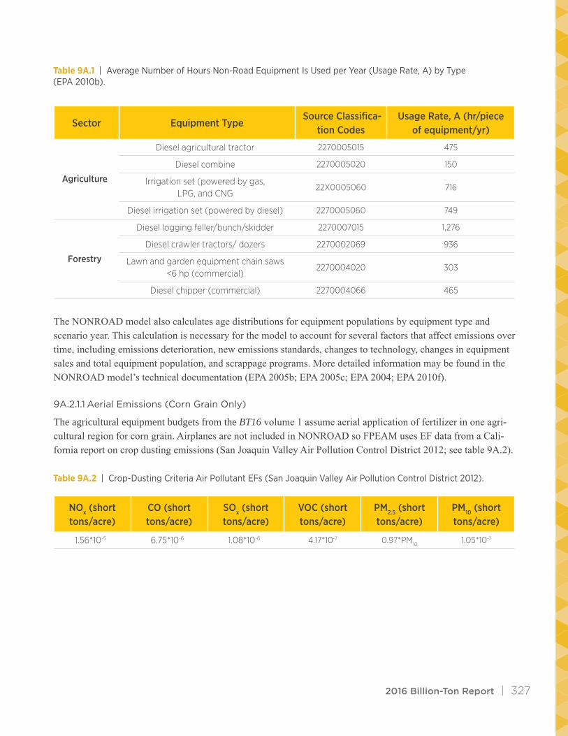
2016 Billion-Ton Report | 327
Table 9A.1 | Average Number of Hours Non-Road Equipment Is Used per Year (Usage Rate, A) by Type (EPA 2010b).
Table 9A.2 | Crop-Dusting Criteria Air Pollutant EFs (San Joaquin Valley Air Pollution Control District 2012).
Sector Equipment Type Source Classifica-
tion CodesUsage Rate, A (hr/piece
of equipment/yr)
Agriculture
Diesel agricultural tractor 2270005015 475
Diesel combine 2270005020 150
Irrigation set (powered by gas, LPG, and CNG
22X0005060 716
Diesel irrigation set (powered by diesel) 2270005060 749
Forestry
Diesel logging feller/bunch/skidder 2270007015 1,276
Diesel crawler tractors/ dozers 2270002069 936
Lawn and garden equipment chain saws <6 hp (commercial)
2270004020 303
Diesel chipper (commercial) 2270004066 465
The NONROAD model also calculates age distributions for equipment populations by equipment type and scenario year. This calculation is necessary for the model to account for several factors that affect emissions over time, including emissions deterioration, new emissions standards, changes to technology, changes in equipment sales and total equipment population, and scrappage programs. More detailed information may be found in the NONROAD model’s technical documentation (EPA 2005b; EPA 2005c; EPA 2004; EPA 2010f).
9A.2.1.1 Aerial Emissions (Corn Grain Only)
The agricultural equipment budgets from the BT16 volume 1 assume aerial application of fertilizer in one agri-cultural region for corn grain. Airplanes are not included in NONROAD so FPEAM uses EF data from a Cali-fornia report on crop dusting emissions (San Joaquin Valley Air Pollution Control District 2012; see table 9A.2).
NOx (short tons/acre)
CO (short tons/acre)
SOx (short tons/acre)
VOC (short tons/acre)
PM2.5 (short tons/acre)
PM10 (short tons/acre)
1.56*10-5 6.75*10-6 1.08*10-6 4.17*10-7 0.97*PM10 1.05*10-7

ImPlIcAtIons oF AIr PollutAnt EmIssIons From ProducIng AgrIculturAl And ForEstry FEEdstocks
328 | 2016 Billion-Ton Report
Table 9A.3 | Conversion Factors for Computing Emissions of NH3, PM2.5, and VOCs Using NONROAD Estimates, which Include PM10 and THCs. LHV Is the Lower Heating Value of the Fuel andNH3 Is the EF for NH3.
The total amount of combustion exhaust emissions, Eaerial,p,cg,c (in lb/yr), for pollutant (P) in each county (c) for corn grain, cg, are given by equation 9A.6.
Equation 9A.6:
Ep, aerial,c,g,c = EFp * Harvc,g,c * 2000
Where the following are defined as
• EFP is the pollutant-specific emission factor from table 9A.2• Harvcg,c is the number of corn grain acres harvested per year in county c (ac/yr)• 2000 converts tons to pounds.
9A.2.1.2 NH3, PM2.5, and Volatile Organic Compound (VOC) Emissions
Since NONROAD does not compute the emissions of NH3, particulate matter under 2.5 micrometers in diameter (PM2.5), or VOCs, we computed these emissions separately using EPA conversion factors (see table 9A.3).
PM2.5
LHV (Btu/gallon)
EF NH3 (g/mm BTU)
VOC
Diesel 0.97*PM10a 128,490c 0.68d 1.053*THCe
Gasoline 0.92*PM10b 116,090c 1.01d 0.933*THCe
LPG 1.0*PM10b 84,450c (not reported) 0.995*THCe
CNG 1.0*PM10b 20,160c (not reported) 0.004*THCe
a EPA 2010d
b EPA 2010e
c DOE 2012
d EPA 2015b
e EPA 2010a
2016 Billion-Ton Report | 329
Emissions of NH3 (ENH3,c,feed in lb/yr for feedsock, feed, in county c) are estimated based on fuel consumption and are given by equation 9A.7.
Equation 9A.7:
ENH3,feed,c = FCfeed * LHV * EFNH3 * 0.0022
Where the following are defined as
• FC is the amount of fuel consumed by the equipment used for feedstock, feed, per year (estimated from NONROAD)
• LHV is the lower heating value of the fuel (Btu/gal) given in table 9A.3• EFNH
3 is the EF for NH3 (g/mmBtu) given in table 9A.3
• 0.0022 is the conversion from grams to pounds.
The size distribution of the particulate matter is given in NONROAD technical documentation (EPA 2010d; EPA 2010e). As shown in table 9A.3, PM2.5 emissions are derived from PM10 and are distinguished by fuel type (EPA 2010c).
The NONROAD program adds THC to oxygenated compounds (alcohols and aldehydes commonly found in engine exhaust) then subtracts the methane and ethane components to get VOC (EPA 2010a). The definition of VOC excludes methane, ethane, acetone, and compounds not commonly found in large quantities in engine ex-haust, like chlorohydrocarbons. Although acetone is not subtracted, it is present in smaller quantities compared to methane and ethane, and will have a negligible effect on the results (EPA 2010a; EPA 2010g). The THC to VOC conversion factors are shown in table 9A.3.
9A.2.2 On-Road Fuel Use Emission Estimates
In consultation with experts at Oak Ridge National Laboratory, we assume that all on-road (off-farm) transpor-tation (i.e., transport of the feedstock from the farm to the depot and the depot to the biorefinery in the long-term logistics case, and transport from the farm to the biorefinery in the near-term case) will occur via a combination short-haul truck (DOE 2016). Although the exact route of travel is unknown, for our modeling purposes, we assume that it would occur within the biomass source county (see limitations discussion in chapter 9, section 9.4.2.2). FPEAM uses EPA’s MOVES model, version 2014a, to estimate the emissions generated during trans-portation using a vehicle of this type (EPA 2016a).
In order to compute the total emissions generated in each county, FPEAM runs MOVES on the county level using the rates mode. This approach allows us to run MOVES once per state and year to compute the emission rates for the county producing the most cellulosic biomass in each state and year. The results are then post-pro-cessed on the county level by combining the appropriate state-level emission rates with the county-level trans-portation data. This approach allows us to compute the total emissions for each feedstock at the county level, while saving valuable computation time by running MOVES only once per state and year for all feedstocks.
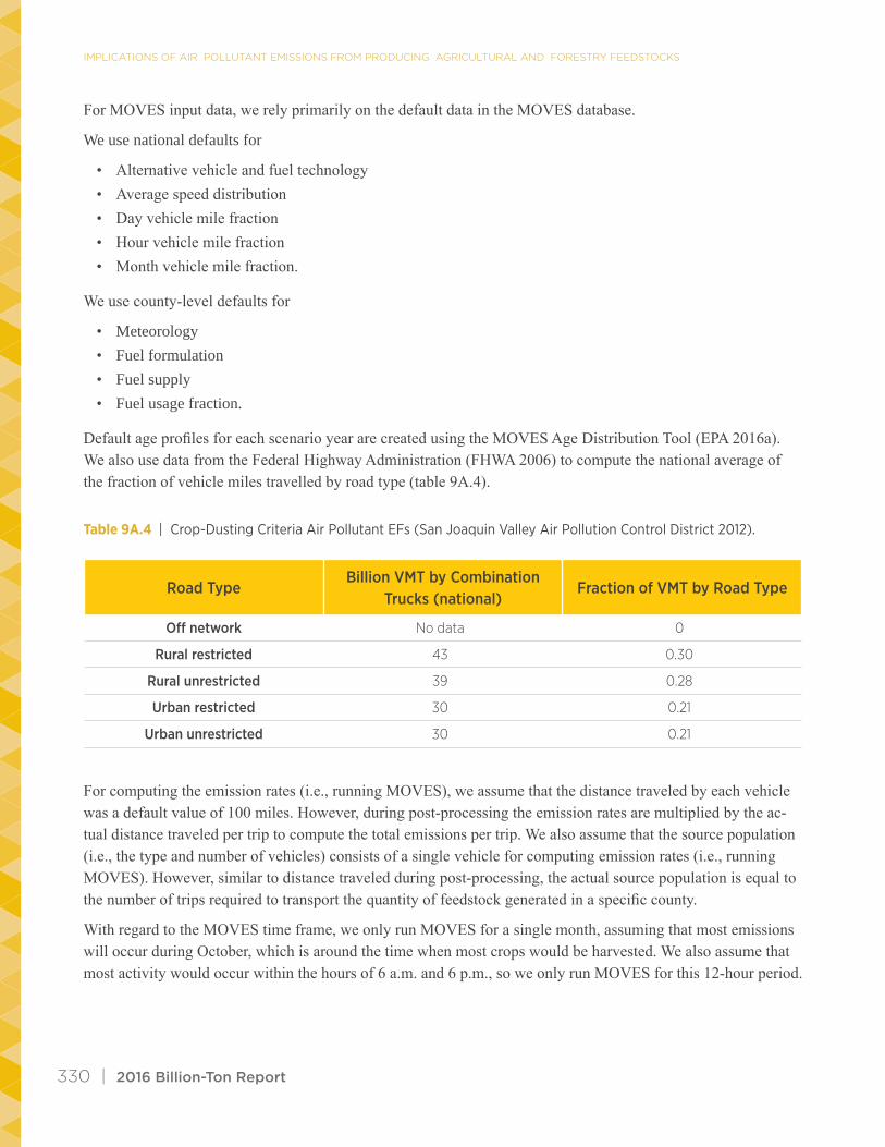
ImPlIcAtIons oF AIr PollutAnt EmIssIons From ProducIng AgrIculturAl And ForEstry FEEdstocks
330 | 2016 Billion-Ton Report
For MOVES input data, we rely primarily on the default data in the MOVES database.
We use national defaults for
• Alternative vehicle and fuel technology• Average speed distribution• Day vehicle mile fraction• Hour vehicle mile fraction• Month vehicle mile fraction.
We use county-level defaults for
• Meteorology• Fuel formulation• Fuel supply• Fuel usage fraction.
Default age profiles for each scenario year are created using the MOVES Age Distribution Tool (EPA 2016a). We also use data from the Federal Highway Administration (FHWA 2006) to compute the national average of the fraction of vehicle miles travelled by road type (table 9A.4).
Table 9A.4 | Crop-Dusting Criteria Air Pollutant EFs (San Joaquin Valley Air Pollution Control District 2012).
Road TypeBillion VMT by Combination
Trucks (national)Fraction of VMT by Road Type
Off network No data 0
Rural restricted 43 0.30
Rural unrestricted 39 0.28
Urban restricted 30 0.21
Urban unrestricted 30 0.21
For computing the emission rates (i.e., running MOVES), we assume that the distance traveled by each vehicle was a default value of 100 miles. However, during post-processing the emission rates are multiplied by the ac-tual distance traveled per trip to compute the total emissions per trip. We also assume that the source population (i.e., the type and number of vehicles) consists of a single vehicle for computing emission rates (i.e., running MOVES). However, similar to distance traveled during post-processing, the actual source population is equal to the number of trips required to transport the quantity of feedstock generated in a specific county.
With regard to the MOVES time frame, we only run MOVES for a single month, assuming that most emissions will occur during October, which is around the time when most crops would be harvested. We also assume that most activity would occur within the hours of 6 a.m. and 6 p.m., so we only run MOVES for this 12-hour period.

2016 Billion-Ton Report | 331
We use the emission rates generated by MOVES (EPA 2015a) to compute the total emissions (EP,f,feed,c in lb/yr) generated by the transportation of each feedstock, feed, in each county, c, according to equation 9A.8.
Equation 9A.8:
EP,f,feed,c =∑h ∑proc ([VP,proc,h,st + PP,proc,h,st+∑r ∑s[DP,r,s,h,proc,st *Sr, s, h * VMTfeed,c,r]]) (Tfeed,c)*2204
Where the following are defined as
• VP,proc,h is the rate per vehicle (in metric tons per vehicle) computed by MOVES for each pollutant, P, pol-lutant process, proc, and hour, h, for the state-level representative county, st, producing the most cellulosic biomass in the state where county, c, resides
• PP,proc,h is the rate per profile (in metric tons per hour)3 computed by MOVES for each pollutant, P, pollut-ant process, proc, and hour, h, for the state-level representative county, st, producing the most cellulosic biomass in the state where county, c, resides
• DP,r,s,h,proc is the rate per distance (in metric tons per vehicle mile travelled) computed by MOVES for each pollutant, P, road type, r, speed bin, s, hour, h, and pollutant process, proc, for the state-level representative county, st, producing the most cellulosic biomass in the state where county, c, resides
• Sr,s,h is the average fractional amount of time that a combination short-haul truck spends traveling on road type, r, in speed bin, s, during hour, h, of a weekday (MOVES default value)
• VMTfeed,c,r is the number of vehicle miles a truck must travel per trip for feedstock, feed, in county, c, on road type, r (DOE 2016)
• Tfeed,c is the number of trips per year required to transport all of feedstock, feed, supplied in county, c (computed from data in DOE 2016)
• 2204 converts from metric tons to pounds.
9A.2.3 Preprocessing Fuel Use and Electricity Emission Calculations
For biomass supply logistics, the only piece of equipment that uses diesel (DOE 2016) is the wood chipper, which is only used for woody feedstocks. We use the NONROAD model (EPA 2010b) to calculate combus-tion exhaust emissions from wood chipping following the same general methods outlined in appendix section 9A.2.1. The exception to these methods are that the population of the wood chipper, POPfeed,c (number of pieces of equipment used for feedstock, feed, in county c), is given by equation 9A.9 rather than by equation 9A.5.
Equation 9A.9:
1
DTPHfeed
1
APOPfeed, c = Supplyfeed, c **
3 Since we are using only diesel powered trucks, and MOVES assumes diesel fuel generates no resting evaporative emissions, the rate per profile is zero.

ImPlIcAtIons oF AIr PollutAnt EmIssIons From ProducIng AgrIculturAl And ForEstry FEEdstocks
332 | 2016 Billion-Ton Report
Other preprocessing equipment uses electricity instead of diesel. Electricity use creates non-local criteria air pollutant emissions upstream of where the electricity is used. As noted in chapter 9, section 9.2.2, we do not evaluate criteria air pollutant emissions from sources upstream of equipment or fertilizer production. However, preprocessing equipment’s primary electricity use is potentially a source of non-local emissions from primary energy use. For discussion, we provide a rough estimate of emissions from electricity use in two counties: an agricultural biomass producing county and a whole-tree biomass producing county. We compare these emissions from electricity use to other emission sources in chapter 9, section 9.3.4.3.
For a single county, c, and for each feedstock category, FC (woody or herbaceous), the emission rate of pollut-ant, P, generated from all preprocessing activities (ERelec,P,FC,c in lb per dt) are calculated by summing emissions over all fuel combustion technologies, such that we have equation 9A.10.
Equation 9A.10:
Eelec,P,FC,c = ∑ Mtech * EFP,tech, * EPHFC,c * 0.0022
Where the following are defined as
• Mtech is the percentage of electricity in the United States supplied by a given technology (see table 9A.5)• EFP,tech are technology specific EFs (g/kWh) (see table 9A.6) • EPHFC,c is the electricity used to process a dt of feedstock category, FC, in county, c (kWh/dt)• 0.0022 is the conversion from grams to pounds.
Table 9A.5’s electricity generation mix provides a general indication of the potential regional variability in these emission estimates.

2016 Billion-Ton Report | 333
Table 9A.5 | Electricity Generation Mix in 2016 of Combustion and Non-Combustion Technologies in the Eight Contiguous North American Electric Reliability Corporation Regions (ANL 2015)
Table 9A.6 | National Electricity Criteria Air Pollutant EFs in 2010 (ANL 2013)
Fuel
Uni
ted
Stat
es
Flor
ida
Relia
bilit
y
Coor
dina
ting
Coun
cil
Mid
wes
t Rel
iabi
lity
Org
aniz
atio
n
Nor
thea
st P
ower
Co
ordi
natin
g Co
unci
l
Relia
bilit
y Fi
rst
Corp
orat
ion
SER
C Re
liabi
lity
Corp
orat
ion
Sout
hwes
t Pow
er P
ool
Texa
s Re
liabi
lity
Entit
y
Wes
tern
Ele
ctric
ity
Coor
dina
ting
Coun
cil
Residual oil 0.6% 1.7% 0.2% 1.4% 0.2% 0.4% 1.3% 0.1% 0.2%
Natural gas 26.4% 60.2% 2.6% 50.1% 15.9% 18.8% 22.7% 41.3% 32.5%
Coal 40% 23.3% 61.8% 2.6% 51.3% 49.3% 56.0% 36.0% 25.4%
Biomass 0.3% 0.5% 0.6% 0.6% 0.1% 0.4% 0.0% 0.2% 0.2%
Non-combustion technologies
32.8% 14.2% 34.7% 45.3% 32.4% 31.0% 20.0% 22.3% 41.7%
Fuel TechnologyNOx
(g/kWh)SOx
(g/kWh)PM10
(g/kWh)PM2.5
(g/kWh)CO
(g/kWh)VOC
(g/kWh)
OilSteam turbine
4.4825 7.6442 0.1797 0.1395 0.1676 0.0216
Natural gasCombined
cycle0.1175 0.0041 0.0009 0.0009 0.098 0.0018
CoalSteam turbine
1.141 3.1998 0.2836 0.1994 0.1221 0.0147
BiomassSteam turbine
0.9267 0.603 2.814 1.9763 4.7546 0.1349
Non-combustion technologies
0 0 0 0 0 0

ImPlIcAtIons oF AIr PollutAnt EmIssIons From ProducIng AgrIculturAl And ForEstry FEEdstocks
334 | 2016 Billion-Ton Report
Table 9A.7 | Share of N Fertilizers, by Type (from USDA 2010), for Each Feedstock.
9A.2.4 Emissions from Chemical Application
The application of fertilizers and pesticides results in the emission of several types of air pollutants, including NH3, NOX, and VOCs. The sections below describe the methods that FPEAM uses to calculate air pollutant emissions from each of these sources.
9A.2.5 Fertilizer Emissions
Our estimates of air pollutant emissions from fertilizer application are limited to the emissions associated with nitrogen fertilizer because no studies have yet reported the emissions of NOX, VOC, SO2, PM2.5, PM10, NH3, or CO from the application of potassium and phosphorus fertilizers. However, fugitive dust emissions from apply-ing these fertilizers are accounted for as described in appendix section 9A.2.5.
Since we do not have information about the exact type of nitrogen fertilizer that is applied to each feedstock, we consider a distribution of the five most commonly used nitrogen fertilizers: anhydrous ammonia, ammonium nitrate, urea, ammonium sulfate, and nitrogen solutions (USDA 2013). We assume these five nitrogennitrogen fertilizers are used for corn grain, stover, straw, switchgrass, and miscanthus.
Because each nitrogen fertilizer type emits different levels of NOX and NH3, we assume the share of each nitro-gen fertilizer among total N usage is identical to that in 2010 (USDA 2010). For switchgrass and miscanthus, N solutions will likely be the primary fertilizers used in the model year (Turhollow 2011) and are assumed to be the only nitrogen fertilizers applied to switchgrass and miscanthus in this analysis. No additional nitrogen fertilizer is assumed necessary for feedstocks from the forestry sector. The fractional share of nitrogen fertilizer applied to each crop is listed in table 9A.7.
Type of FertilizerFractional Share of nitrogen
Fertilizer (Nshare) for CG, CS, and WSFractional Share of nitrogen
Fertilizer (Nshare) for SG and MS
Anhydrous ammonia 0.34 0
Ammonium nitrate 0.03 0
Urea 0.25 0
Ammonium sulfate 0.03 0
Nitrogen solutions 0.35 1
Acronyms: CG = corn grain; CS = corn stover; WS = wheat straw; SG = switchgrass; and MS = miscanthus.

2016 Billion-Ton Report | 335
For all feedstocks, the fertilizer-specific EF, in pounds of NO or NH3 per pound of N (lb pollutant/lb N) applied, are given by equation 9A.11 and equation 9A.12.
Equation 9A.11:
%VNO
100
30
14EFNO,F = ( () )
Equation 9A.12:
%VNH3
100
17
14EFNH3,F
= ( () )Where the following are defined as
• F is the type of fertilizer• % VNO or NH3 is the percentage of N in the fertilizer that is volatized as NO or NH3 (100% * lb pollutant/lb
N provided in table 9A.8)• The factors 30/14 and 17/14, respectively, convert the amount of N to NO and NH3 via the molecular
weight of the pollutant versus that of N.
Table 9A.8 | N content (EPA 2015b) and the Amount of N Volatilized as Nitric Oxide (% VNO from EPA 2015b and ANL 2015) and NH3 (% VNH3 )from EPA 2015b and Davidson et al. 2004) for Five Types of Commonly Used N Fertilizers.
Type of Fertilizer N Content (%) %VNO %V NH3
Anhydrous ammonia 82 0.79 4.0
Ammonium nitrate 36 3.8 1.91
Urea 46 0.9 15.8
Ammonium sulfate 22 3.5 9.53
Nitrogen solutions 29 0.79 8.0

ImPlIcAtIons oF AIr PollutAnt EmIssIons From ProducIng AgrIculturAl And ForEstry FEEdstocks
336 | 2016 Billion-Ton Report
For stover and straw, the amount of emissions of pollutant, P, from fertilizer, F, for feedstock, feed, in county, c, (in lb/yr) is given by equation 9A.13.
Equation 9A.13:
EP,F,feed,c = Prodfeed,c * Napp,feed,c * Nshare,F * EFP,F
Where the following are defined as
• Prodfeed,c is the amount of feedstock, feed, produced in dt in county, c, per year• Napp,feed,c is the amount of N applied in pounds per dt of feedstock, feed, in county, c• Nshare,F is the share of N in fertilizer, F, as compared to all fertilizers in pounds of N in F per pound of N in
all fertilizers (given in table 9A.7)• EFP,F is the emission factor for pollutant, P, from fertilizer, F, in pounds of pollutant per pound of N in F
(given by the equation 9A.11 and equation 9A.12).
For corn grain, switchgrass, and miscanthus the amount of emissions E_(P,F,c) (in lb/yr) generated by pollutant, P, from fertilizer, F, in county, c, is given by equation 9A.14.
Equation 9A.14:
EP,F,feed,c = Harvfeed,c * Napp,feed,c * Nshare,F * EFP,F
Where the following are defined as
• Harvfeed,c is the amount acreage of feedstock, feed, harvested in acres per year in county, c (DOE 2016)• Napp,feed,c is the amount of N applied in county, c, in pounds per harvested acre of feedstock, feed (DOE
2016)• Nshare,F is the share of N in fertilizer, F, as compared to all fertilizers in pounds of N in F per pound of N in
all fertilizers (given in table 9A.7)• EFP,F is the emission factor for pollutant, P, from fertilizer, F, in pounds of pollutant per pound of N in F
(given by the equation 9A.11 and equation 9A.12).
For each type of feedstock, the total amount of emissions of pollutant, P, associated with feedstock, feed, in county, c, EP,fert,feed,c (in lb/year), from all fertilizer application is calculated by summing emissions over all five types of fertilizers, such that we have equation 9A.15.
Equation 9A.15:
EP, fert, feed, c = ∑EP, Fi , feed, c
5
i=1

2016 Billion-Ton Report | 337
Where the following are defined as
• EP,Fi,feed,c is the amount of emissions of pollutant, P, from fertilizer, Fi, associated with feedsock, feed, in county, c, given by equation 9A.13 or 9A.14
• F1 is anhydrous ammonia• F2 is ammonium nitrate• F3 is urea• F4 is ammonium sulfate• F5 is N solutions.
9A.2.6 Pesticide Emissions
The application of pesticides (e.g., herbicides, insecticides, and fungicides) results in the emission of VOCs. The estimation of emissions from pesticides is challenging due to the wide range of formulations (e.g., emulsi-fiable concentrate, aerosol, solution, flowable, granule), application equipment, and application type (e.g., band, broadcast, serial, spot). Although the Emission Inventory Improvement Program (EIIP) describes the preferred methodology for computing the amount of emissions generated by pesticide application (EPA 2001), this methodology requires a large amount of information that was unavailable for this study. As a result, we used the method used in the 2011 National Emission Inventory (Huntley 2015). According to this method, the total pesti-cide emissions, Epest,feed,c (in lb of VOC per year in county, c), by feedstock, feed, are given by equation 9A.16.
Equation 9A.16:
Epest, feed, c = Harv feed, c * R feed, c * ER * CVOC
Where the following are defined as
• Harvfeed,c is the harvested acreage of feedstock, feed, in county, c• Rfeed,c is the amount of pesticide applied to feedstock, feed, per harvested acre in county, c (lb pesticide/acre)
(DOE 2016)• ER is the evaporation rate (ratio; default value = 0.9)• CVOC is the VOC content (lb VOC/lb active ingredient; default value = 0.835).
9A.2.7 Fugitive Dust Emissions
We assume that there are no fugitive dust emissions from preprocessing equipment at the biorefinery in the near-term system or at the depot in the long-term system because the design cases that serve as the basis for equipment preprocessing assumptions used in Supply Characterization Model (SCM) modeling (DOE 2016) have a baghouse or other emission control system in place (INL 2013; INL 2014). Although whole-tree biomass and residue chipping are likely to generate fugitive emissions, no EFs for fugitive dust were identified for the operation.
ImPlIcAtIons oF AIr PollutAnt EmIssIons From ProducIng AgrIculturAl And ForEstry FEEdstocks
338 | 2016 Billion-Ton Report
After reviewing the literature and having discussions with regulatory experts at EPA, the California Air Resourc-es Board (CARB), and researchers at the Consortium for Research on Renewable Industrial Materials (COR-RIM), we concluded that data and methods are not currently available for estimating fugitive dust from forestry sector biomass production (chapter 9, section 9.4.2.3).
9A.2.7.1 Agriculture Harvest and Non-Harvest Activities
Agricultural activities include airborne soil PM emissions produced during the preparation of agricultural lands for planting, harvesting, and other activities. For example, dust emissions are produced by the mechanical distur-bance of the soil by the implement used and the tractor pulling it (WRAP 2006).
According to research performed at the University of California, Davis, and summarized by CARB (Gaffney and Yu 2003; CARB 2003), the EFs for all types of agricultural land preparation (non-harvest) activities can be classified into one of five categories (table 9A.9). Additional EFs were also reported (by feedstock type) for harvest activities associated with three crop types (CARB 2003; table 9A.10).
Table 9A.9 | EFs for Fugitive Emissions of PM Generated by Agricultural Non-Harvest Activities (Gaffney and Yu 2003).
Table 9A.10 | EFs for Fugitive Emissions of PM Associated with Harvesting Cotton, Wheat, and Almonds (CARB 2003).
Category Emission Factor (lbs PM10/acre-pass)
Root cutting 0.3
Discing, tilling, chiseling 1.2
Ripping, subsoiling 4.6
Land planning and floating 12.5
Weeding 0.8
Harvest Operation Emission Factor (lbs PM10/acre)
Cotton picking 1.7
Cotton stalking 1.7
Cotton total 3.4
Wheat combining 5.8
Wheat total 5.8
Almond shaking 0.37
Almond sweeping 3.7
First almond pickup 36.7
Almond total 40.8

2016 Billion-Ton Report | 339
In consultation with agricultural experts, CARB (2003) used scaling factors to expand its analysis and approxi-mate EFs for other crops (see table 9A.11 for scaling factors associated with FPEAM feedstocks). Since harvest EFs tend to be fairly unique for each crop, all harvest operations were combined into a single factor that includ-ed all relevant operations (CARB 2003). As a result, harvest EFs are reported per acre rather than per acre-pass. Although the scaling factors for corn grain and wheat came directly from CARB (2003), switchgrass and corn stover were not included so we assumed that these crops would be similar to corn grain (table 9A.11).
Table 9A.11 | EFs for Fugitive Emissions of PM Generated by Agricultural Harvest Activities Associated with FPEAM Feedstocks (Derived from CARB 2003).
Feedstock Type Scaling Factor Crop ProxyEmission Factor (lbs PM10/acre)
Corn grain 0.5a Cotton total 1.7
Corn stover 0.5b Cotton total 1.7
Wheat straw 1a Wheat total 5.8
Switchgrass 0.5b Cotton total 1.7
Miscanthus 0.5b Cotton total 1.7
a CARB 2003
b Assumed similar to corn grain
We classified each of the non-harvest activities into the categories outlined in table 9A.9. We then used these EFs for each category to compute the fugitive dust emissions for each type of machinery in pounds of PM10 per acre of feedstock (see tables 9A.12–9A.16). By summing the estimated emissions generated from all field activities, we evaluated the total fugitive dust emissions associated with harvest and non-harvest activities for all feedstock types (see table 9A.17). Due to the product-purpose allocation approach that we use for corn stover and wheat straw, there are no non-harvest fugitive dust emissions associated with these two crops. We only incorporate the additional emissions that would result from additional crop harvesting activities for corn stover and wheat straw.

ImPlIcAtIons oF AIr PollutAnt EmIssIons From ProducIng AgrIculturAl And ForEstry FEEdstocks
340 | 2016 Billion-Ton Report
Table 9A.12 | EFs for Fugitive Emissions of PM for Non-Harvest Activities Associated with Switchgrass (Derived from Gaffney and Yu 2003 and National Crop Budgets in Zhang et al. 2016).
Table 9A.13 | EFs for Fugitive Emissions of PM for Non-Harvest Activities Associated with Conventional Till Corn Grain (Derived from Gaffney and Yu 2003 and National Crop Budgets in Zhang et al. 2016).
Category Field Activity Passes Over FieldFugitive Dust
Emissions (lbs PM10/acre)
Establishment – Year 1
Discing, tilling, chiseling Offset disk 2 2.4
Weeding Fertilizer and lime spreader 2 1.6
Weeding Boom sprayer 3 2.4
Discing, tilling, chiseling No-till drill 1 1.2
Maintenance – Years 2–10
Discing, tilling, chiseling Reseeding (year 2 only) 1 1.2
Weeding Fertilizer and lime spreader 1 0.8
Weeding Boom sprayer, 50 ft (year 5 only) 1 0.8
Category Field Activity Passes Over FieldFugitive Dust
Emissions (lbs PM10/acre)
Weeding Dry fertilizer spreader 1 0.8
Weeding Chemical applicator GE 30ft 1 0.8
Weeding Chemical applicator GE 30ft 1 0.8
Weeding Fertilizer applicator 1 0.8
Discing, tilling, chiseling Eight-row planter 1 1.2
Discing, tilling, chiseling Field cultivator 1 1.2
Discing, tilling, chiseling Tandem disk 1 1.2
Discing, tilling, chiseling Moldboard plow 1 1.2

2016 Billion-Ton Report | 341
Table 9A.14 | EFs for Fugitive Emissions of PM10 for Non-Harvest Activities Associated with Reduced Till Corn Grain (Derived from Gaffney and Yu 2003 and National Crop Budgets in Zhang et al. 2016).
Category Field Activity Passes Over FieldFugitive Dust
Emissions (lbs PM10/acre)
Weeding Dry fertilizer spreader 1 0.8
Weeding Dry fertilizer spreader 1 0.8
Discing, tilling, chiseling Row cultivator 1 1.2
Discing, tilling, chiseling Eight-row planter 1 1.2
Weeding Chemical applicator 1 0.8
Discing, tilling, chiseling Tandem disk 1 1.2
Discing, tilling, chiseling Offset disk/light duty 1 1.2
Category Field Activity Passes Over FieldFugitive Dust Emis-
sions (lbs PM10/acre)
Weeding Dry fertilizer spreader 1 0.8
Weeding Dry fertilizer spreader 1 0.8
Weeding Chemical applicator 1 0.8
Weeding Dry fertilizer spreader 1 0.8
Weeding Chemical applicator 1 0.8
Discing, tilling, chiseling Seven-row no-till planter 1 1.2
ImPlIcAtIons oF AIr PollutAnt EmIssIons From ProducIng AgrIculturAl And ForEstry FEEdstocks
342 | 2016 Billion-Ton Report
Table 9A.16 | EFs for Fugitive Emissions of PM10 for Non-Harvest Activities Associated with Miscanthus (Derived from Gaffney and Yu 2003, Mari et al. 2002, and National Crop Budgets in Zhang et al. 2016).
Category Field Activity Passes Over FieldFugitive Dust
Emissions (lbs PM10/acre)
Establishment – Year 1
Weeding Mower 1 0.8
Discing, tilling, chiseling Offset disk 2 2.4
Ripping, subsoiling Ripper bedder (deep tillage) 1 4.6
Weeding Fertilizer and lime spreader 2 1.6
Weeding Boom sprayer 3 2.4
Discing, tilling, chiseling Potato planter 1 1.2
Maintenance – Years 2–10
Weeding Fertilizer and lime spreader 1 0.8
Weeding Boom sprayer, 50 ft (year 5 only) 1 0.8
By summing the emissions over all of the machinery used during each year, we compute the total PM10 per acre of feedstock harvested (tables 9A.12–9A.16). As shown, the emissions vary with tillage method for corn grain. The total harvest and non-harvest fugitive dust emissions of PM10 , EPM10,FDharv/nonharv,c, (in lb/yr) for each feedstock, feed, in county, c, are given by equation 9A.17.
Equation 9A.17:
EPM10, FDharv/nonharv, feed, c = Harv feed, c * (EFfeed,Harv,T + EFfeed, Nonharv)
Where the following are defined as
• Harvfeed,c is the amount of harvested area of feedstock, feed, in county, c, per year (acre/yr)• EFfeed,Harv and EFfeed,Nonharv are EFs (lb/acre) for feedstock, feed, from tables 9A.17–9A.19 by tillage type.
Based on the Midwest Research Institute (MRI 2006), we assume that the ratio of PM2.5 to PM10 for fugitive dust emissions is 0.2.

2016 Billion-Ton Report | 343
Table 9A.17 | Total PM10 Fugitive Dust Emissions Associated with Harvest and Non-Harvest Activities for Corn Grain, Corn Stover, and Wheat Straw (Derived from Gaffney and Yu 2003, CARB 2003, and National Crop Budgets in Zhang et al. 2016).
Table 9A.18 | Total PM10 Fugitive Dust Emissions Associated with Harvest and Non-Harvest Activities for Mis-canthus (Derived from Gaffney and Yu 2003, CARB 2003, and National Crop Budgets in Zhang et al. 2016).
Table 9A.19 | Total PM10 Fugitive Dust Emissions Associated with Harvest and Non-Harvest Activities for Switch-grass (Derived from Gaffney and Yu 2003, CARB 2003, and National Crop Budgets in Zhang et al. 2016).
Corn Grain (lbs PM10/ac) Stover
(lbs PM10/ac)Straw
(lbs PM10/ac)Conventional Till
Reduced Till
No-Till
Non-Harvest 8 7.2 5.2 – –
Harvest 1.7 1.7 1.7 1.7 5.8
YearTotal Emissions (lbs PM10/acre)
Harvest Non-Harvest
1 1.7 13
2 1.7 1.6
2–15 1.7 0.8
YearTotal Emissions (lbs PM10/acre)
Harvest Non-Harvest
1 1.7 7.6
2 1.7 2
3–4 1.7 0.8
5 1.7 1.6
6–10 1.7 0.8

ImPlIcAtIons oF AIr PollutAnt EmIssIons From ProducIng AgrIculturAl And ForEstry FEEdstocks
344 | 2016 Billion-Ton Report
Table 9A.20 | Biomass Supply Logistics Distances, where Total Distance Traveled (D) Is Split among Each Road Type (INL 2016).
9A.2.7.2 Transportation on All Roads
EPA has established methods for estimating fugitive dust emissions from road travel, which vary by road type (EPA 2006). The number of miles traveled by road type (e.g., unpaved, primary paved, and secondary paved) for biomass transportation were not available from BT16 volume 1. As a result, we used national averages to estimate distances traveled on each road type (INL 2016). For each feedstock in each county, we subdivided the total distance traveled, D, during biomass supply logistics (DOE 2016) by road type based on the national average in table 9A.20.
Variable Agricultural Feedstocks Forestry Feedstocks
Dunpaved D < 2 miles D < 10 miles
Dsecondary paved
D > 2 miles D > 10 miles
D < 50 miles D < 50 miles
Dprimary paved D > 50 miles D > 50 miles
9A.2.7.3 Transportation on Unpaved Roads
According to EPA (2006), for vehicles traveling on unpaved surfaces under similar conditions to those found at industrial sites (i.e., surface silt content of 1.8%–25.2%, mean vehicle weight from 2–290 tons and mean vehicle speed from 5–43 mph), the fugitive dust emission rate (ERFDunpaved,st in state, st, in lb per vehicle mile traveled) are given by equation 9A.18.
Equation 9A.18:
sst
12
W
3ERFDunpaved,st = k ( () )
a b
Where the following are defined as
• k, a, and b are empirical constants listed in table 9A.21• sst is the surface material silt content (percentage; values vary by state, st, according to EPA 2006)• W is the mean weight of the vehicles on the road (3.2 tons) (FHWA 2000).

2016 Billion-Ton Report | 345
Table 9A.21 | Empirical Constants Used for Determining Fugitive Dust Emissions from Unpaved Industrial Roads (EPA 2006).
Constant PM10 PM2.5
k (lb/VMT) 1.5 0.15
A 0.9 0.9
B 0.45 0.45
Acronyms: lb = pounds; VMT = vehicle miles traveled
Equation 9A.18 was modified for use in FPEAM to estimate the total amount of fugitive dust emissions of pollutant, P (PM10 or PM2.5), generated by transportation on unpaved roads in county, c, EP,FDunpaved,feed,c (in lb per year), for each feedstock in each biomass supply logistics system and is given by equation 8A.19.
Equation 9A.19:
sst
12
Supply feed,c
Cfeed
W
3Eunpaved, FD, feed, c = * Dunpaved, feed* k ( )( () )ap bp
Where the following are defined as
• Supplyfeed,c is the amount of feedstock, feed, supplied per year in county, c (dt/yr)• C is the capacity of the truck hauling the feedstock (dt/load)• Dunpaved,feed is the distance that feedstock, feed, travels in vehicle miles traveled on unpaved roads (mi) (see
table 9A.20)• sst and W are given by equation 9A.18• kP, aP, and bP are the constants for pollutant, P (see table 9A.21).
9A.2.7.4 Transportation on Paved Roads
According to EPA (2011), for vehicles traveling on paved surfaces, the fugitive dust emission rate (ERP,FDpaved,c) in lb of pollutant, P, per vehicle mile travelled in county, c) are given by equation 9A.20.
Equation 9A.20:
ERP,FDpaved,c = kP * sLap * Wbp

ImPlIcAtIons oF AIr PollutAnt EmIssIons From ProducIng AgrIculturAl And ForEstry FEEdstocks
346 | 2016 Billion-Ton Report
Table 9A.22 | Empirical Constant Used for Determining Fugitive Dust Emissions from Paved Industrial Roads (EPA 2011).
Acronyms: lb = pounds; VMT = vehicle miles traveled
Where the following are defined as
• kP,,aP,and bP are empirical constants listed in table 9A.22 for pollutant, P• sL is the road surface silt loading (g/m2) on secondary (0.4 g/m2) and primary (0.045 g/m2) paved roads• W is the mean weight of the vehicles on the road (3.2 tons) (FHWA 2000).
Constant PM10 PM2.5
k (lb/VMT) 0.0022 0.00054
A 0.91 0.91
B 1.02 1.02
Equation 9A.21:
Supply feed,c
Cfeed
Supply feed,c
Cfeed
EP,FDsec unpaved, FD, feed, c = * Dsec unpaved, feed* kP * sLsecap * Wbp
EP,FDpri unpaved, FD, feed, c = * Dpri unpaved, feed* kP * sLpriap * Wbp
Equation 9A.22:
Where the following are defined as
• Supplyfeed,c is the amount of feedstock, feed, supplied per year in county, c (dt/yr)• Cfeed is the capacity of the truck hauling feedstock, feed (dt/load)• kP, aP, and bP are given by equation 9A.20• sLsec and sLpri are the road surface silt loading (g/m2) on secondary and primary paved roads, respectively
(see equation 9A.20)• Dsecpaved,feed and Dpri paved,feed are the distances that feedstock, feed, travels in vehicle miles traveled on second-
ary and primary paved roads (mi), respectively (see table 9A.20).

2016 Billion-Ton Report | 347
9A.2.7.5 Limitations of Transport Fugitive Dust Calculations
There are two main limitations to the paved road fugitive dust equations described above. First, these equations were derived using a regression analysis of experimental data, including 83 road tests on public, paved, and controlled and uncontrolled industrial paved roads. Second, these conditions may not be representative of the source conditions used in our analysis as performance is based on equipment used in the 1970s. The paved road fugitive dust equations were found to be of good quality using EPA’s AP-42 data quality scoring system (score of A) for the range of source conditions listed in table 9A.23, which encompasses the source conditions used in our analysis.
The unpaved road fugitive dust equations were also determined empirically and are considered to be of fairly high quality by EPA (score of B) under certain source conditions. Like the paved road equations, the source conditions for the unpaved road fugitive emissions equation align fairly well with the scenario conditions (table 9A.24).
However, these equations do not include a reduction factor for precipitation, which is known to have an impact of fugitive dust generation. The AP-42 does provide an equation for paved road fugitive dust emissions that
ParameterRange of Source Conditions Where the
Equations are Deemed to be High Quality
Range of Source Conditions Employed for Biomass
Transportation Analysis
Silt loading (g/m2) 0.03–400 0.045 (primary), 0.4 (secondary)
Mean vehicle weight (Mt) 1.8–38 3.2
ParameterRange of Source Conditions Where the
Equations are Deemed to be High Quality
Range of Source Conditions Employed for Biomass
Transportation Analysis
Silt loading (%) 1.8–25.2 0-7.2a
Mean vehicle weight (Mt) 1.8–260 3.2
Table 9A.23 | Comparison of Source Condition Ranges Where the Fugitive Dust Equations Are To Be Deemed of High Quality and Where Biomass Transportation Is Expected to Occur for Paved Roads (EPA 2011; equation 9A.20).
Table 9A.24 | Comparison of Source Condition Ranges Where the Fugitive Dust Equations Are To Be Deemed of High Quality and Where Biomass Transportation Is Expected to Occur for Unpaved Roads (EPA 2006; equation 9A.18).
includes a precipitation correction term. However, this precipitation correction equation has not been rigorous-ly verified and is considered to be of lower quality than the standard equation. As a result, we use the equation without the precipitation correction factor.
a EPA Unpaved Road Surface Material Silt Content Values used in the 1999 NEI (https://www3.epa.gov/ttn/chief/ap42/ch13/relat-ed/c13s02-2.html)

ImPlIcAtIons oF AIr PollutAnt EmIssIons From ProducIng AgrIculturAl And ForEstry FEEdstocks
348 | 2016 Billion-Ton Report
Several other limitations of the fugitive dust emission equations relate to data availability. For example, silt content varies spatially, and the data are not readily available to identify the silt content for unpaved roads for each county. As a result, we use constant values for silt content for primary and secondary paved roads and state averages for unpaved roads (EPA 2006). In addition, we use national data to estimate the fractional amount of travel that occurs on each road type. However, in practice, the distance travelled on each road type would likely vary widely on a county level.
Finally, it is important to note that we only report source emissions of fugitive dust. We do not account for the fraction of particulate matter that might be deposited or dispersed by surrounding vegetation or other roughness elements near the source. Several studies indicate that the fraction of particulate matter relevant to air quality analyses may be much smaller than the source emissions (Watson and Chow 2000; Cowherd, Grelinger, and Gebhart 2005; Pace 2005; Pardyjak et al. 2008; Janhäll 2015). Thus, if our results are used in air quality models, potential transportable fractions (e.g., fractions described in the 2011 air quality modeling platform for National Emissions Inventory (NEI) data (EPA 2015c)) should be considered.
9A.2.7.6 Preprocessing Fugitive Dust Sensitivity Analysis
As noted in chapter 9, section 9.2.2, we assume fugitive dust from preprocessing equipment to be zero due to the dust collection systems assumed to be in place in both near-term and long-term supply logistics designs (INL 2013; INL 2014). In section 9.3.4.3 of chapter 9, we discuss and compare the emissions of 99% dust collection to other sources of PM emissions. According to EPA (1999), baghouse air pollution control technologies may not be completely (or 99.9% complete) effective at dust collection due to the age of the equipment or whether a high-quality enclosed system is installed.
We estimate potential emissions of PM10 and PM2.5 based on the following equations and data taken from Krause and Smith (2006). For a single county, and for each feedstock category, FC (woody or herbaceous), the particu-late emissions from preprocessing4 (ERpreprocess FD in lb/dt) are calculated by equation 9A.23.
Equation 9A.23:
Where the following are defined as
• PRFC is the processing throughput rate for the feedstock category, FC• gL is 0.004 (grain loadings/ft3) (WLA Consulting 2011)• 1/7000 (lbs/grains) is a constant• The assumed Air Flow Rate is 51,0005 (scfm) (Davis et al. 2013)
1
7000EFpreprocess PM, FC = PRFC * gL * * Air Flow Rate * 60 * 8760
4 All PM is assumed to be less than 10 μm in diameter. PM2.5 emissions are assumed to be 17% of PM10 emissions (WLA Consulting 2011).
2016 Billion-Ton Report | 349
• 60 (min/hr) is a constant• 8,760 (hrs/yr) is a constant.
9A.2.8 Other Emissions from Preprocessing and Drying
The preprocessing and drying of woody feedstocks is expected to generate VOC emissions. Based on the INL (2013, 2014) design reports, which are used as the basis for biomass supply logistics in SCM modeling (DOE 2016), the near-term and long-term logistics systems use an indirect heat rotary dryer and a cross-flow dryer, respectively. They also both use a hammer mill for preprocessing.
We used EPA’s (2002) VOC EFs for wood preprocessing and drying equipment to estimate these emissions. EPA provides VOC EFs for rotary dryers and hammer mills, but not for cross-flow dryers. Mechanically, the convey-or dryer in EPA (2002) most closely resembles the cross-flow dryer but not in terms of the drying temperature. Therefore, we use the conveyor dryer EFs that assume the use of a regenerative catalytic oxidizer in order to approximate potential VOC emissions. Table 9A.25 summarizes the softwood and hardwood EFs that FPEAM uses to estimate VOC emissions from drying a 50/50 split mixedwood.
For each feedstock in each biomass supply logistics system, the total amount of VOC emissions generated by drying and preprocessing in county, c (EDrying and preprocessing,c in lb/yr), is given by equation 9A.24.
Equation 9A.24:
Where the following are defined as
• Supplyfeed,c is the amount of feedstock, feed, supplied to biorefineries in county, c (dt/yr) (DOE 2016)• EFdrying and EFmilling are VOC emission factors (kg/dt) (see table 9A.25)• 2.2 converts kg to lb.
EDrying and Preprocessing, feed = Supplyfeed, c * (EFdrying +EFmilling) * 2.2
5 51,000 (8,500 x 6 baghouse) is used for a facility.

ImPlIcAtIons oF AIr PollutAnt EmIssIons From ProducIng AgrIculturAl And ForEstry FEEdstocks
350 | 2016 Billion-Ton Report
EquipmentBiomass Supply Logistics System
Softwood EF (kg/dt)
Hardwood EF (kg/dt)
50/50 Mixed Wood EF (used
in Eq S22) (kg/dt)
Indirect Heat Rotary Dryer Near-Term 0.92 0.13 0.53
Conveyor6 Natural Gas Dryer Heating and Cooling
ZonesLong-Term 0.41 0.034 0.23
Flaker/Refinery/ Hammer Mill
Near-Term and Long-Term
– – 0.52
Table 9A.25 | Softwood, Hardwood, and Mixedwood VOC EFs from EPA (2002).
9A.3 Supplemental Results
9A.3.1 SOx, NOx, and COFigure 9A.1 shows the locations of counties in nonattainment with the National Ambient Air Quality Standards (NAAQS) for SO2 for the two BC1&ML scenarios. Upwind travel of SO2 emissions is limited, so only changes in SO2 in nonattainment areas (NAAs) are discussed in the main chapter.
No county is out of compliance with the current NO2 and CO NAAQS (EPA 2016b), so we display maps (fig. 9A.2 and 9A.3) to illustrate the spatial distribution of county-level emission ratio. In the 2040 scenario, the max-imum change in the NEI ratio for attainment counties for CO from BT16 biomass production and supply scenar-ios is 3%. The maximum change in the NEI ratio for producing biomass is 18%. Counties having NO2 emission ratios greater than 18% is the result of transporting biomass long distances to multiple surrounding counties for biofuel production. Due to the limitations of our analysis, all emissions from those long transportation distances are allocated to the biomass producing counties, and therefore interpretation of these high values is not possible with the long distance biomass traveled.
6 VOC EFs for a cross-flow grain dryer are not available from EPA. Expert consultation indicated the conveyor dryer was a close approximate.

2016 Billion-Ton Report | 351
Figure 9A.1 | BC1&ML 2017 and 2040 scenarios’ county-level distributions of emission ratios for SO2 (top frame).7 Maps of emission ratios and nonattainment counties at the end of 2015 exceeding NAAQS standards for SO2 (prima-ry, 1-hour) (EPA 2016c)8 are displayed in red in the 2017 (middle frame) and 2040 (bottom frame) maps. Box and whisker plots represent minimum, 25th percentile, median, 75th percentile, and maximum.
7 See the main text for a complete list of counties in partial nonattainment with emission ratios above 1%.8 Includes NAA designations for the 1971 and 2010 NAAQS. Includes NAA designations EPA maintains based on prior year
standards. EPA considers older standards for certain pollutants and we follow EPA in this respect.

ImPlIcAtIons oF AIr PollutAnt EmIssIons From ProducIng AgrIculturAl And ForEstry FEEdstocks
352 | 2016 Billion-Ton Report
Figure 9A.2 | BC1&ML 2017 and 2040 scenarios’ county-level distributions of emission ratios for NO2 (top frame). Maps of emission ratios and nonattainment counties at the end of 2015 exceeding NAAQS standards for NO2 (primary, 1-hour, and 1-year) (EPA 2016c)9 are displayed in red in the 2017 (middle frame) and 2040 (bottom frame) maps. Box and whis-ker plots represent minimum, 25th percentile, median, 75th percentile, and maximum.
9 Includes NAA designations for the 1971 NAAQS.

2016 Billion-Ton Report | 353
Figure 9A.3 | BC1&ML 2017 and 2040 scenarios’ county-level distributions of emission ratios for CO (top frame). Maps of emission ratios and nonattainment counties at the end of 2015 exceeding NAAQS standards for CO (pri-mary, 8-hour, and 1-hour) (EPA 2016c)10 are displayed in red in the 2017 (middle frame) and 2040 (bottom frame) maps. Box and whisker plots represent minimum, 25th percentile, median, 75th percentile, and maximum.
10 Includes NAA designations for the 1971 NAAQS.

ImPlIcAtIons oF AIr PollutAnt EmIssIons From ProducIng AgrIculturAl And ForEstry FEEdstocks
354 | 2016 Billion-Ton Report
9A.3.2 High Yield
Figures 9A.4–9A.9 compare the BC1&ML 2040 scenario to the HH3&HH 2040 scenarios.

2016 Billion-Ton Report | 355
Figure 9A.4 | BC1&ML and HH3&HH 2040 scenarios’ county-level distributions of emission ratios for ozone (top frame).11 Maps of emission ratios and nonattainment counties at the end of 2015 exceeding NAAQS standards for ozone (primary, 8-hour) (EPA 2016c)12 are displayed in red in the BC1&ML (middle frame) and HH3&HH (bottom frame) maps. Box and whisker plots represent minimum, 25th percentile, median, 75th percentile, and maximum.
11 See the main text for a complete list of nonattainment counties with emission ratios above 1%.12 Includes NAA designations for the 2008 NAAQS that are still in force.

ImPlIcAtIons oF AIr PollutAnt EmIssIons From ProducIng AgrIculturAl And ForEstry FEEdstocks
356 | 2016 Billion-Ton Report
Figure 9A.5 | BC1&ML and HH3&HH 2040 scenarios’ county-level distributions of emission ratios for PM2.5 (top frame). Maps of emission ratios and nonattainment counties at the end of 2015 exceeding NAAQS standards for PM2.5 (primary, 24-hour, and 1-year) (EPA 2016c) are displayed in red in the BC1&ML (middle frame) and HH3&HH (bottom frame) maps. Box and whisker plots represent minimum, 25th percentile, median, 75th percentile, and maximum.
13 See the main text for a complete list of nonattainment counties with emission ratios above 1%.14 Includes NAA designations for the 1997, 2006, and 2012 NAAQS that are still in force..

2016 Billion-Ton Report | 357
Figure 9A.6 | BC1&ML and HH3&HH 2040 scenarios’ county-level distributions of emission ratios for PM10 (top frame).15 Maps of emission ratios and nonattainment counties at the end of 2015 exceeding NAAQS standards for PM10 (primary, 24-hour) (EPA 2016c)16 are displayed in red in the BC1&ML (middle frame) and HH3&HH (bottom frame) maps. Box and whisker plots represent minimum, 25th percentile, median, 75th percentile, and maximum.
15 See the main text for a complete list of nonattainment counties with emission ratios above 1%.16 Includes NAA designations for the 1987 and 2012 NAAQS that are still in force.

ImPlIcAtIons oF AIr PollutAnt EmIssIons From ProducIng AgrIculturAl And ForEstry FEEdstocks
358 | 2016 Billion-Ton Report
Figure 9A.7 | BC1&ML and HH3&HH 2040 scenarios’ county-level distributions of emission ratios for SO2 (top frame).17 Maps of emission ratios and nonattainment counties at the end of 2015 exceeding NAAQS standards for SO2 (primary, 1-hour) (EPA 2016c)18 are displayed in red in the BC1&ML (middle frame) and HH3&HH (bottom frame) maps. Box and whisker plots represent minimum, 25th percentile, median, 75th percentile, and maximum.
17 See the main text for a complete list of counties in partial nonattainment with emission ratios above 1%.18 Includes NAA designations for the 1971 and 2010 NAAQS that are still in force.
.
2016 Billion-Ton Report | 359
Figure 9A.8 | BC1&ML and HH3&HH 2040 scenarios’ county-level distributions of emission ratios for NO2 (top frame). Maps of emission ratios and nonattainment counties at the end of 2015 exceeding NAAQS standards for NO2 (primary, 1-hour, and 1-year) (EPA 2016c)19 are displayed in red in the BC1&ML (middle frame) and HH3&HH (bottom frame) maps. Box and whisker plots represent minimum, 25th percentile, median, 75th percentile, and maximum.
19 Includes NAA designations for the 1971 NAAQS that are still in force..

ImPlIcAtIons oF AIr PollutAnt EmIssIons From ProducIng AgrIculturAl And ForEstry FEEdstocks
360 | 2016 Billion-Ton Report
Figure 9A.9 | BC1&ML and HH3&HH 2040 scenarios’ county-level distributions of emission ratios for CO (top frame). Maps of emission ratios and nonattainment counties at the end of 2015 exceeding NAAQS standards for CO (primary, 8-hour, and 1-hour) (EPA 2016c)20 are displayed in red in the BC1&ML (middle frame) and HH3&HH (bottom frame) maps. Box and whisker plots represent minimum, 25th percentile, median, 75th percentile, and maximum.
20 Includes NAA designations for the 1971 NAAQS that are still in force.

2016 Billion-Ton Report | 361
9A.4 ReferencesArgonne National Laboratory (ANL). 2013. Updated Greenhouse Gas and Criteria Air Pollutant Emission
Factors of the U.S. Electric Generating Units in 2010. Lemont, IL: Systems Assessment Section, Energy Systems Division, Argonne National Laboratory. https://greet.es.anl.gov/publication-electricity-13.
———. 2015. GREET Model 2015. Accessed June 2016. https://greet.es.anl.gov/.
CARB (California Air Resources Board). 2003. “Section 7.5 – Agricultural Harvest Operations.” Accessed June 2016. http://www.arb.ca.gov/ei/areasrc/fullpdf/full7-5.pdf.
———. 2006. “Appendix D – Emission Inventory Methodology, Agricultural Irrigation Pumps – Diesel.” http://www.arb.ca.gov/regact/agen06/attach2.pdf.
Cowherd, C., Jr., Mary Ann Grelinger, and Dick L. Gebhart. 2005. “Development of an Emission Reduction Term for Near-Source Depletion.” Proceedings of the Air and Waste Management Association's Annual Conference and Exhibition. https://www3.epa.gov/ttnchie1/conference/ei15/session5/cowherd.pdf.
Davidson, Cliff, Peter Adams, Ross Strader, Rob Pinder, Natalie Anderson, Marian Geobes, and Josh Ayers. 2004. CMU Ammonia Emission Inventory for the Continental United States, version 3.6. Pittsburgh, PA: The Environmental Institute, Carnegie Mellon University. http://www.cmu.edu/ammonia/.
Davis, R., L. Tao, E. C. D. Tan, M. J. Biddy, G. T. Beckham, C. Scarlata, J. Jacobson, K. Cafferty, J. Ross, J. Lu-kas, D. Knorr, and P. Schoen. 2013. Process Design and Economics for the Conversion of Lignocellulosic Biomass to Hydrocarbons: Dilute-Acid and Enzymatic Deconstruction of Biomass to Sugars and Biologi-cal Conversion of Sugars to Hydrocarbons. National Renewable Energy Laboratory: Golden, CO. NREL/TP-5100-60223. http://www.nrel.gov/docs/fy14osti/60223.
DOE (U.S. Department of Energy). 2011. U.S. Billion-Ton Update: Biomass Supply for a Bioenergy and Bio-products Industry. Oak Ridge, TN: Oak Ridge National Laboratory. ORNL/TM-2011/224.http://energy.gov/eere/bioenergy/downloads/us-billion-ton-update-biomass-supply-bioenergy-and-bioproducts-industry.
———. 2012. “Alternative Fuels Data Center: Fuel Properties Comparison.” DOE, Office of Energy Efficiency and Renewable Energy. www.afdc.energy.gov/afdc/fuels/properties.html.
———. 2016. U.S. Billion-Ton Report: Advancing Domestic Resources for a Thriving Bioeconomy, Volume 1: Economic Availability of Feedstocks. Oak Ridge, TN: Oak Ridge National Laboratory. ORNL/TM-2016/160. http://energy.gov/sites/prod/files/2016/07/f33/2016_billion_ton_report_0.pdf.
EPA (Environmental Protection Agency). 1999. “Air Pollution Control Technology Fact Sheet,” EPA. EPA-452/F-03-025. https://www3.epa.gov/ttnchie1/mkb/documents/ff-pulse.pdf.
———. 2001. “Chapter 9: Pesticides – Agricultural and Nonagricultural.” In Emission Inventory Improvement Program (EIIP) Technical Report Series, Volume III: Area Sources and Area Source Method Abstracts. Durham, NC: EPA, EIIP. https://www.epa.gov/sites/production/files/2015-08/documents/iii09_jun2001.pdf.
———. 2002. “Chapter 10: Wood Products Industry.” In AP 42: Compilation of Air Emission Factors, Fifth Edition, Volume 1. https://www3.epa.gov/ttnchie1/ap42/ch10/.

ImPlIcAtIons oF AIr PollutAnt EmIssIons From ProducIng AgrIculturAl And ForEstry FEEdstocks
362 | 2016 Billion-Ton Report
———. 2004. Nonroad Engine Growth Estimates. Washington, DC: EPA, Office of Transportation and Air Quality, Assessment and Standards Division. EPA420-P-04-008. https://www3.epa.gov/otaq/models/non-rdmdl/nonrdmdl2004/420p04008.pdf.
———. 2005a. User’s Guide for the Final NONROAD2005 Model. Washington, DC: EPA, Office of Transpor-tation and Air Quality, Assessment and Standards Division. EPA420-R-05-013. https://nepis.epa.gov/Exe/ZyPDF.cgi?Dockey=P1004L24.pdf.
———. 2005b. Exhaust Emission Effects of Fuel Sulfur and Oxygen on Gasoline Nonroad Engines. Wash-ington, DC: EPA, Office of Transportation and Air Quality, Assessment and Standards Division. EPA420-R-05-016. https://www3.epa.gov/otaq/models/nonrdmdl/nonrdmdl2005/420r05016.pdf.
———. 2005c. Calculation of Age Distributions in the Nonroad Model: Growth and Scrappage. Washington, DC: Office of Transportation and Air Quality, Assessment and Standards Division. EPA420-R-05-018. https://www3.epa.gov/otaq/models/nonrdmdl/nonrdmdl2005/420r05018.pdf.
———. 2006. “Chapter 13: Miscellaneous Sources.” In AP 42: Compilation of Air Emission Factors, Fifth Edi-tion, Volume 1. https://www3.epa.gov/ttnchie1/ap42/ch13/.
———. 2010a. Conversion Factors for Hydrocarbon Emission Components. Washington, DC: EPA, Office of Transportation and Air Quality, Assessment and Standards Division. EPA-420-R-10-015. https://www3.epa.gov/otaq/models/nonrdmdl/nonrdmdl2010/420r10015.pdf.
———. 2010b. Median Life, Annual Activity, and Load Factor Values for Nonroad Engine Emissions Model-ing. Washington, DC: EPA, Office of Transportation and Air Quality, Assessment and Standards Division. EPA-420-R-10-016. https://www3.epa.gov/otaq/models/nonrdmdl/nonrdmdl2010/420r10016.pdf.
———. 2010c. Nonroad Engine Population Estimates. Washington, DC: EPA, Office of Transportation and Air Quality, Assessment and Standards Division. EPA-420-R-10-017. https://www3.epa.gov/otaq/models/nonrdmdl/nonrdmdl2010/420r10017.pdf.
———. 2010d. Exhaust and Crankcase Emission Factors for Nonroad Engine Modeling – Compression-Igni-tion. Washington, DC: EPA, Office of Transportation and Air Quality, Assessment and Standards Division. EPA-420-R-10-018. https://www3.epa.gov/otaq/models/nonrdmdl/nonrdmdl2010/420r10018.pdf.
———. 2010e. Exhaust Emission Factors for Nonroad Engine Modeling – Spark-Ignition. Washington, DC: EPA, Office of Transportation and Air Quality, Assessment and Standards Division. EPA-420-R-10-019. https://www3.epa.gov/otaq/models/nonrdmdl/nonrdmdl2010/420r10019.pdf.
———. 2010f. Nonroad Spark-Ignition Engine Emission Deterioration Factors. Washington, DC: EPA, Office of Transportation and Air Quality, Assessment and Standards Division. EPA-420-R-10-020. https://www3.epa.gov/otaq/models/nonrdmdl/nonrdmdl2010/420r10020.pdf.
———. 2010g. Nonroad Evaporative Emission Rates. Washington, DC: EPA, Office of Transportation and Air Quality, Assessment and Standards Division. EPA-420-R-10-021. https://www3.epa.gov/otaq/models/nonrdmdl/nonrdmdl2010/420r10021.pdf.
———. 2011. “Chapter 13: Miscellaneous Sources.” In AP 42: Compilation of Air Emission Factors, Fifth Edi-tion, Volume 1. https://www3.epa.gov/ttnchie1/ap42/ch13/.

2016 Billion-Ton Report | 363
———. 2015a. Air Toxic Emissions from On-road Vehicles in MOVES2014. Washington, DC: EPA, Office of Transportation and Air Quality, Assessment and Standards Division. EPA-420-R-15-021. https://nepis.epa.gov/Exe/ZyPDF.cgi?Dockey=P100NOGN.pdf.
———. 2015b. 2011 National Emissions Inventory, version 2, Technical Support Document. Research Triangle Park, NC: EPA, Office of Air Quality Planning and Standards, Air Quality Assessment Division, Emis-sions Inventory and Analysis Group. https://www.epa.gov/sites/production/files/2015-10/documents/nei2011v2_tsd_14aug2015.pdf.
———. 2015c. Preparation of Emissions Inventories for the Version 6.2, 2011 Emissions Modeling Platform, Technical Support Document. Research Triangle Park, NC: EPA, Office of Air and Radiation/Office of Air Quality Planning and Standards, Air Quality Assessment Division. https://www.epa.gov/sites/production/files/2015-10/documents/2011v6_2_2017_2025_emismod_tsd_aug2015.pdf.
———. 2016a. MOVES (MOtor Vehicle Emission Simulator). Accessed June 2016. https://www.epa.gov/moves.
———. 2016b. “Modeling and Inventories: NONROAD Model (Nonroad Engines, Equipment, and Vehicles).” https://www.epa.gov/moves/nonroad-model-nonroad-engines-equipment-and-vehicles.
———. 2016c. Nonattainment Areas for Criteria Pollutants (Green Book). https://www.epa.gov/green-book.
FHWA (Federal Highway Administration). 2000. “Chapter 3: Truck Fleet and Operations.” In Comprehensive Truck Size and Weight Study, volume 2. http://www.fhwa.dot.gov/reports/tswstudy/Vol2-Chapter3.pdf.
——. 2006. Annual Vehicle Distance Traveled in Miles and Related Data – 2006, by Highway Category and Vehicle Type Table. http://www.fhwa.dot.gov/policy/ohim/hs06/pdf/vm1.pdf.
Gaffney, Patrick, and Hong Yu. 2003. “Computing Agricultural PM10 Fugitive Dust Emissions Using Process Specific Emission Rates and GIS.” Paper presented at the U.S. EPA Annual Emission Inventory Confer-ence, San Diego, CA. Accessed June 2016. www.epa.gov/ttnchie1/conference/ei12/fugdust/yu.pdf.
Huntley, R. 2015. 2011 National Emissions Inventory (NEI) methodology documentation. Research Triangle Park, NC: Emission Inventory and Analysis Group, EPA. https://www.epa.gov/air-emissions-invento-ries/2011-nei-technical-support-document.
INL (Idaho National Laboratory). 2013. Feedstock Supply System Design and Economics for Conversion of Lig-nocellulosic Biomass to Hydrocarbon Fuels – Conversion Pathway: Biological Conversion of Sugars to Hydrocarbons – “The 2017 Design Case.” Idaho Falls, ID: INL, Bioenergy Program. INL/EXT-13-30342. https://inldigitallibrary.inl.gov/sti/6013245.pdf.
———. 2014. “” Feedstock Supply System Design and Economics for Conversion of Lignocellulosic Biomass to Hydrocarbon Fuels – Conversion Pathway: Fast Pyrolysis and Hydrotreating Bio-oil Pathway – “The 2017 Design Case.” Idaho Falls, ID: INL, Bioenergy Program. INL/EXT-14-31211. https://inldigitalli-brary.inl.gov/sti/6038147.pdf.
———. 2016. “Approximate national average transportation distance traveled on unpaved, primary paved, and secondary paved roads.” (Personal communication with author on January 21).

ImPlIcAtIons oF AIr PollutAnt EmIssIons From ProducIng AgrIculturAl And ForEstry FEEdstocks
364 | 2016 Billion-Ton Report
Janhäll, Sara. 2015. “Review on urban vegetation and particle air pollution – Deposition and dispersion.” Atmo-spheric Environment 105:130–7. doi:10.1016/j.atmosenv.2015.01.052.
Krause, Mike, and Steve Smith. 2006. “Final – Methodology to Calculate Particulate Matter (PM) 2.5 and PM 2.5 Significance Thresholds.” Diamond Bar, CA: South Coast Air Quality Management District. nitrogen fertilizer
Mari, G. R., S. A. Memon, N. Leghari, and A. D. Brohi. 2002. “Evaluation of Tractor Operated Potato Planter.” Pakistan Journal of Applied Sciences 2 (9): 889–91. http://docsdrive.com/pdfs/ansinet/jas/2002/889-891.pdf.
MRI (Midwest Research Institute). 2006. Background Document for Revisions to Fine Fraction Ratios Used for AP-42 Fugitive Dust Emission Factors. Prepared for the Western Governors’ Association, Western Re-gional Air Partnership. MRI Project No. 110397. http://www.epa.gov/ttnchie1/ap42/ch13/bgdocs/b13s02.pdf.
Pace, Thompson G. 2005. “Methodology to Estimate the Transportable Fraction (TF) of Fugitive Dust Emis-sions for Regional and Urban Scale Air Quality Analyses.” U.S. Environmental Protection Agency. http://www.nrc.gov/docs/ML1321/ML13213A386.pdf.
Pardyjak, E. R., S. O. Speckart, F. Yin, and J. M. Veranth. 2008. “Near source deposition of vehicle generated fugitive dust on vegetation and buildings: Model development and theory.” Atmospheric Environment 42 (26): 6442–52. doi:10.1016/j.atmosenv.2008.04.024.
San Joaquin Valley Air Pollution Control District. 2012. 2012 Area Source Emissions Inventory Methodology: 810 Civilian Aircraft. San Joaquin Valley Air Pollution Control District. https://www.valleyair.org/Air_Quality_Plans/EmissionsMethods/MethodForms/Current/CivilianAircraft2012.pdf.
Turhollow, A. 2011. “Switchgrass crop management and harvesting equipment requirements”. Oak Ridge Na-tional Laboratory. (Personal Communication with A. Carpenter on July 14).
USDA (U.S. Department of Agriculture). 2009. “2008 Farm and Ranch Irrigation Survey.” USDA Census of Agriculture. http://www.agcensus.usda.gov/Publications/2007/Online_Highlights/Farm_and_Ranch_Irri-gation_Survey/index.php.
———. 2010. “Table 4: U.S. consumption of selected nitrogen materials.” Fertilizer Use and Price. USDA, Eco-nomic Research Service. http://www.ers.usda.gov/webdocs/DataFiles/Fertilizer_Use_and_Price__17978//fertilizeruse.xls.
———. 2013. “Table 5: U.S. Consumption of nitrogen, phosphate, and potash.” Fertilizer Use and Price. USDA, Economic Research Service. http://www.ers.usda.gov/webdocs/DataFiles/Fertilizer_Use_and_Price__17978//fertilizeruse.xls.
Wang, Michael, Hong Huo, and Sail Arora. 2011. “Methods of dealing with co-products of biofuels in life-cycle analysis and consequent results within the U.S. context.” Energy Policy 39 (10): 5726–36. doi:10.1016/j.enpol.2010.03.052.
Watson, John G., and Judith C. Chow. 2000. Reconciling Urban Fugitive Dust Emissions Inventory and Ambient Source Contribution Estimates:Summary of Current Knowledge and Needed Research. Reno, NV: Desert Research Institute. DRI Document No. 6110.4F. https://www3.epa.gov/ttn/chief/efdocs/fugitivedust.pdf.

2016 Billion-Ton Report | 365
WLA Consulting. 2011. 2011 Updated Facility Design Prevention of Significant Deterioration Air Quality Construction Permit Application. Prepared for Abengoa Bioenergy Biomass of Kansas, LLC. http://www.kdheks.gov/bar/abengoa/ABBK_PSD_App.pdf.
WRAP (Western Regional Air Partnership). 2006. WRAP Fugitive Dust Handbook. Prepared by Countess Envi-ronmental for Western Governors’ Association, WRAP. http://www.wrapair.org/forums/dejf/fdh/content/FDHandbook_Rev_06.pdf.
Zhang, Yimin, Garvin Heath, Alberta Carpenter, and Noah Fisher. 2016. “Air Pollutant Emissions Inventory of Large-Scale Production of Selected Biofuels Feedstocks in 2022.” Biofuels, Bioproducts & Biorefining 10 (1): 56–69. doi:10.1002/bbb.1620.

This page was intentionally left blank.