Proceedings of the 8th International Symposiumon Experimental and ComputationalAerothermodynamics of Internal FlowsLyon, July 2007Paper reference : ISAIF8-0053

Modeling of 3-D Losses and Deviationsin a Throughflow Analysis Tool

Jean-Francois SimonTechspace Aero - Aerodynamic Groupjsimon@techspace-aero.be

Alain NicksUniversity of Liege - Turbomachinery Groupalainnicks@hotmail.com

Nicolas ParisUniversity of Liege - Turbomachinery GroupNicolas.Paris@student.ulg.ac.be

Olivier LeonardUniversity of Liege - Turbomachinery Groupo.leonard@ulg.ac.be

This contribution is dedicated to the modeling of the end-wall flows in a throughflow model for turbomachinery applications.The throughflow model is based on the Euler or Navier-Stokes equations solved by a Finite-Volume technique. Two approaches arepresented for the end-wall modeling. The first one is based on an inviscid formulation with dedicated 3-D distributions of loss coefficientand deviation in the end-wall regions. The second approach is directly based on a viscous formulation with no-slip boundary conditionalong the annular end-walls and blade force modification in the region close to the end-walls. The throughflow results are comparedto a series of 3-D Navier-Stokes calculations averaged in the circumferential direction. These 3-D calculations were performed on thethree rotors of a low pressure axial compressor, for a series of tip clearance values.

Keywords: throughflow, losses, deviations, axial compressors

Introduction

The throughflow level of approximation still remainsan important tool for designing turbomachines [2] eventhough 3-D calculations are used more and more early inthe design process. The throughflow models heavily relyon empirical inputs such as 2-D correlations or end-wallloss models. This feature has shown to be efficient butlacks of generality.

Two-dimensional empirical correlations are availablein the literature but they have generally been designed forclassical families of blade profiles such as C4 or NACA-65 and are not directly applicable to the custom-based pro-files nowadays used in the industry. However, it is possi-ble to adapt existing loss correlations to modern blade pro-files [5] or to derive correlations for an arbitrary profileswith the help of blade-to-blade codes [6].

Concerning the 3-D losses, very few results are avail-

Proceedings of the 8th International Symposium on Experimental and Computational Aerothermodynamics of Internal Flows 2

able in the open literature. The main contribution on thecompressor side is from Roberts et al. [7,8]. They pro-posed correlations based on collected empirical data tobuild up 3-D distributions of loss coefficient and devia-tion in the end-wall regions. A throughflow analysis toolbased on an inviscid model, supplemented with these 3-D correlations for the end-wall losses is the first approachstudied here.

The second approach presented in this contribution isdirectly based on the Navier-Stokes equations with bladeforce modifications close to the end-walls to capture theend-wall flows. By including more physics in the model,less empiricism is needed and a more general method cantherefore be devised.

The objective of the present work is to test both ap-proaches for the modeling of the end-wall flows withina throughflow model. The results are compared to a se-ries of 3-D Navier-Stokes calculations performed on axialcompressor rotors.

Nomenclature

ARc channel aspect ratio, h/sm

c mean blade chordh mean span or mean blade heights blade spacing [mm]S3D extent of 3-D loss, in fraction of span(S3D)max location of maximum 3-D loss, in

fraction of spanTC rotor blade tip clearance, in fraction

of span

Greek lettersδ flow deviation angleδ∗ displacement thicknessσ solidity, c/sφ blade camber angle$ loss coefficientθ flow deflectionR = W2/W1 velocity ratio

Subscripts1 inlet5 5% of span from tip at the blade outlet95 95% of span from tip at the blade outlet2D relative to a two-dimensional flow3D relative to a three-dimensional flowh hubmax maximum locationmo maximum overturning locationrt rotor tip

Throughflow analysis tool

The throughflow analysis tool used in the present workis based on the Euler equations [1,11] and the Navier-Stokes equations [9]. Such models allow to calculate theflow field whatever the flow regime is, they are able toperform transient simulations and they can cope with 2-Dflow recirculations. These approaches offer alternatives tothe classical streamline curvature method.

Details on the present solver are available in [9]. Inshort, the equations are solved by a finite volume tech-nique. The inviscid fluxes are computed thanks to the Roescheme and the viscous flux by the diamond path scheme.The time integration is performed by an explicit multistepRunge-Kutta scheme.

The turbulence model is of the mixing length type anda radial mixing model based on a turbulent diffusion as-sumption is used. The inviscid blade force is computed byan additional time-dependent equation [1], while the vis-cous blade force is calculated by a distributed loss modeland empirical correlations. In order to avoid loss gener-ation by the inviscid blade force, its direction is chosenorthogonal to the flow field. An adaptation of the inviscidblade force in the end-wall regions is therefore required.More details on these modifications are available in a fol-lowing section.

3-D database

The test-case used in the present work is composedof 3 rotors of a low pressure compressor designed byTechspace Aero. For each rotor, four different tip clear-ance values were considered: 0.4, 0.8, 1 and 1.2 percentsof the mean blade height. The database is composed of 3-D Navier-Stokes calculation results. For each configura-tion, two computations were run, one with flow conditionsand blade incidence representative of an on-design con-figuration, a second one representative of near-stall condi-tions. The mesh is made of about 1.2 million grid pointsand the turbulence model is algebraic.

These 3-D Navier-Stokes computations, after a cir-cumferential averaging, provide the boundary conditionsfor the throughflow calculations. Rotor blades were dis-cretized in ten sections at different blade heights to trans-fer the blade camber and thickness to the throughflowanalysis tool in a rather complete way. The radial bladeforces were neglected.

Inviscid annulus end-walls formulation

The first approach for modeling the end-wall flows is

Proceedings of the 8th International Symposium on Experimental and Computational Aerothermodynamics of Internal Flows 3

based on an inviscid treatment of the hub and shroud witha slip condition. The effect of the viscous flow develop-ing along the end-walls is (partly) reintroduced by addinga 3-D distribution of deviation and loss coefficient on thetop of the 2-D distributions:

$ = $2D + $3D (1)δ = δ2D + δ3D (2)

The figure 1 illustrates the 3-D distributions obtainedwith Roberts correlations [7,8] for a rotor. The usual evo-lution of the deviation with an overturning at the hub andan overturning followed by an underturning at the tip isobserved. The loss coefficient distribution also shows aclassical shape at both end-walls.

The expression of Roberts correlations is reproducedhereafter in order to highlight the main parameters drivingthe loss and deviation generation.

0 20 40 60 80 1000

0.02

0.04

0.06

0.08

0.1

(a) Loss coefficient vs blade height

0 20 40 60 80 100−6

−4

−2

0

2

4

(b) Deviation vs blade height

Figure 1 : Original 3-D correlations of Roberts

Correlations for 3D losses at shroud :

($3D)max,rt = 0.25 tanh√

103δ∗1 · TC (3)

(S3D)max,rt =($3D)max,rt

2(4)

(S3D)rt = 2.5(S3D)max,rt (5)

Correlations for 3D losses at hub :

($3D)max = 0.2 tanh

√15(

φ · δ∗21

ARc ·√

σ) (6)

(S3D)max = 0.1 (7)

S3D = 2.5 · (S3D)max = 0.25 (8)

Correlations for 3D deviations at hub :

∆95 = −2 (9)

hh = 0.85 (10)

Correlations for 3D deviations at shroud :

∆5 = 30 tanh(103δ∗1 · TC) (11)

∆mo = −1.25 (12)

hmo = 0.15 (13)

These correlations allow to describe the distributionsof the 3-D loss coefficients and deviations using only afew parameters, the latter being obtained from the flow-path geometry, the blade geometry and the inlet boundarylayer displacement thickness. These parameters howeverdo not allow to obtain the whole distributions along thespan but only some typical points of these distributions.Additional information must be provided. The followingcurves (Gaussian law, 1-D damped oscillator equation andparabola) have been used to connect the points providedby the correlation of Roberts:

f(x) =1

σ√

2πexp

(− (x− µ)2

2σ2

)(14)

f(x) = exp(x

τ

)[f0 cos(ωdx) + β sin(ωdx)] (15)

f(x) = ax2 + bx + c (16)

A last remark has to be added before presenting the re-sults obtained with this approach. The loss coefficient inthe tip region obtained from the 3-D Navier-Stokes com-putations does not always follow the classical distribution

Proceedings of the 8th International Symposium on Experimental and Computational Aerothermodynamics of Internal Flows 4

shown on figure 1(a). Distributions with no peak are ob-tained when the value of the tip clearance is low com-pared to the boundary layer thickness, as shown on figure2, which gives the loss coefficient distribution for differ-ent tip clearance values, for one of the rotors considered inthis work. These distributions with no peak have not beenincluded in the database. Clearly, another way to charac-terize the loss coefficient distribution for low tip clearancevalues is needed.

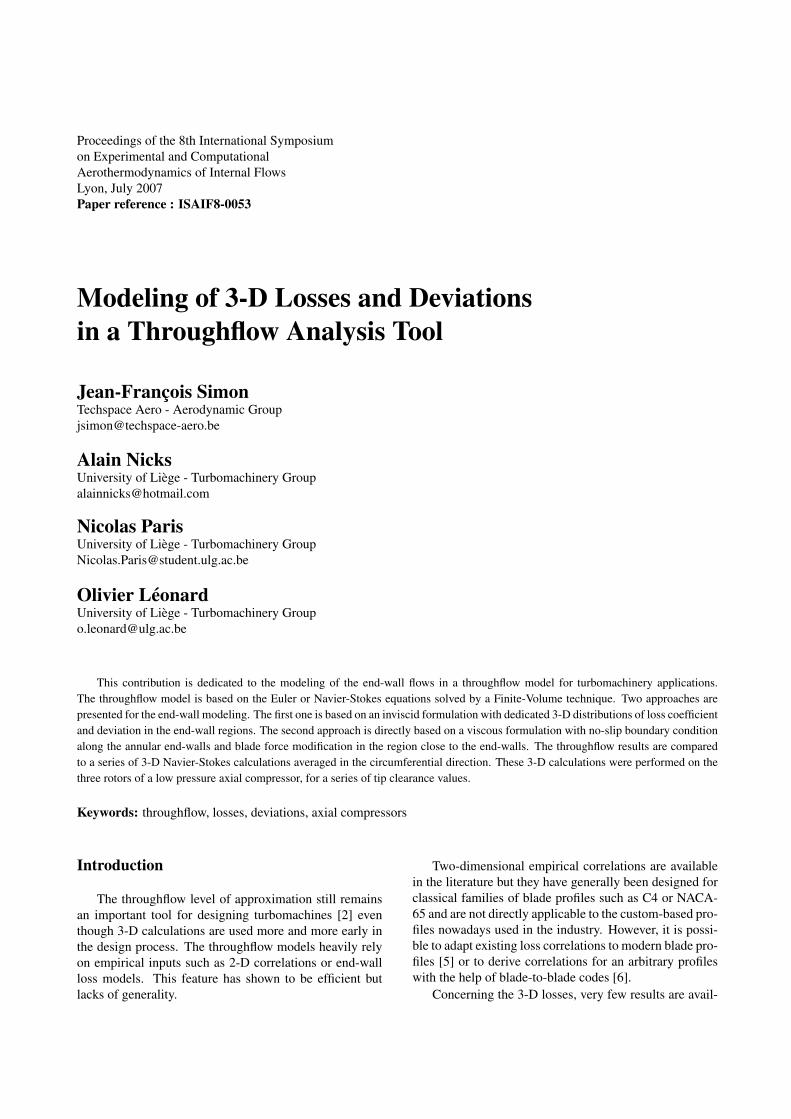
Applying the original correlations provided byRoberts to the rotors considered in the present work failedto reproduce the averaged 3-D Navier-Stokes results. Acalibration procedure was performed on the parametersof Roberts correlations so as to fit the 3-D Navier-Stokesdatabase corresponding to the first rotor blade. The fig-ure 3 compares the loss coefficient distributions in the tipregion obtained with the original correlation, with the cal-ibrated one and with the 3-D averaged one.

Unfortunately applying this calibrated correlation tothe two other rotor geometries failed to reproduce the flowcharacteristics for these rotors, as shown on figure 4. Thisfigure shows one of the parameters of Roberts correlation,($3D)max,rt, i.e. the peak in the 3-D loss coefficient, ver-sus a combination of the clearance gap and the boundarylayer thickness. These results are related to on-design op-erating points only.

The above results demonstrate the need for includingextra parameters in the Roberts correlation in order to takeinto account additional effects such as the blade loading.Indeed the main drawback of Roberts correlations is thatthey do not rely on quantities representative of the aero-dynamic loading (to the exception of the blade camber forthe maximum loss at hub).

From that observation, it was decided to test severalfunctions depending on the loading, the velocity ratio orthe flow deflection in order to derive the sought correla-tions. This was performed systematically for each variableto be modeled by the correlations. The obtained results arepresented hereafter.

The figure 5 illustrates the results obtained for the peakof the loss coefficient distribution in the tip region, for sev-eral rotors and several clearance values. The function usedto approximate it is of the following form :

($3D)max,rt = A tanh(Ra · θb

(1000 · δ∗1 · TC

))(17)

where A, a and b are the parameters determined by thecalibration process. The results are thought to be good.The 3-D Navier-Stokes distributions for which no peaksare observed have also been added on the same figure. Forthese distributions the maximum of the loss coefficient hasbeen used instead of the (non-existing) peak. These valueshave however not been used to build the correlations.

0.8 0.85 0.9 0.95 1

Loss

coe

ffici

ent

Normed radii

TC=0,42%TC=0,84%TC=1,05%TC=1,26%

Figure 2 : Radial distribution of loss coefficient obtainedfrom 3D calculations

Figure 3 : Loss coefficient distribution at rotor tip

0 0.05 0.1 0.15 0.2 0.25 0.3 0.350

0.05

0.1

0.15

0.2

0.25

0.3

0.35

0.4

103δ1* TC/h2

(ϖ3D

) max

,rt

1st rotor2nd rotor3rd rotor1st rotor calibrated correlationoriginal correlation

Figure 4 : Clearance effect fitted on 1st rotor data

Proceedings of the 8th International Symposium on Experimental and Computational Aerothermodynamics of Internal Flows 5

f(R,θ,ARc,δ

1* ,TC)

(ϖ3D

) max

correlationNS 3−D simulation with no peakNS 3−D simulation

Figure 5 : Loss coefficient peak at tip

f(R,φ,ARc,δ

1* ,σ)

(ϖ3D

) max

correlationNS 3−D simulation

Figure 6 : Loss coefficient peak at hub

The figure 6 illustrates the same quantity for the hubregion and again illustrates the quality of the results.

It is recognized that the database used here is far tobe sufficiently dense to allow drawing general correla-tions such as those devised by Roberts. More operat-ing points and more geometries should be considered andtested. However, the proposed procedure, based on load-ing criterions and on 3-D numerical simulations seems tobe promising and should be easily extended to a largerdatabase.

Viscous annulus end-walls formulation

However, it must be recognized that the previousmethod essentially based on empirical correlations lacksof generality. An improved method for capturing the 3-D flows, inspired from Gallimore [4], is proposed here-

after. In the frame of its viscous Streamline Curvaturemethod, Gallimore proposed to modify the blade force(its circumferential component more exactly) in the end-wall regions. The modification he proposed for the bladeforce is based on experimental observations of the bladewall static pressure field, noteworthy the observations ofDring [3]. These results show that the circumferentialcomponent of the blade force varies smoothly across thespan and does not exhibit rapid changes as one approachesthe end-walls contrary to the circumferential momentumjump across the blade row. This is an illustration of thewell known fact that the pressure field does not vary muchacross a boundary layer in the direction orthogonal to thewall.

From that observation it seems possible to extrapolatesome information across the span to model the blade forcein the end-wall regions. A simple model for the evolutionof the circumferential blade force in these regions is pro-posed hereafter for a rotor:

• for the hub flow, the circumferential component ofthe blade force is kept constant over a given portionof the span, starting from the hub,

• for the tip flow, the blade force is set to zero in thegap. The blade force is also kept constant from agiven spanwise position to the tip gap. It was foundthat this last modification is necessary in order toobtain the correct level of underturning in the tipregion. It is in agreement with the experimental ob-servations of Gallimore [4] and Dring [3].

This is a rather simple model and more elaboratedprediction of the evolution of the blade force inside theboundary layer can be devised (see the model of Gal-limore [4] for example). The purpose here is to evaluatethe benefit that such a method could bring on the 3-D lossand deviation predictions.

In the regions where the inviscid blade force is mod-ified, the flow does not follow any more the camber sur-face. In order to avoid the generation of numerical losses,it is important that the blade force remains orthogonal tothe flow. For this reason, it is not possible to work directlyon the modulus of the blade force. To avoid imposing aconstrain on the modulus of the force, the modificationis performed on its circumferential component only. Theother components are computed so that the resulting bladeforce is still orthogonal to the flow field.

The modification of the blade force is tested hereafteron the first rotor studied in the previous section. The flowpath is shown on the figure 7, together with the mesh usedin the present study.

Proceedings of the 8th International Symposium on Experimental and Computational Aerothermodynamics of Internal Flows 6

Figure 7 : Typical mesh used

0 0.05 0.1 0.15 0.2 0.25 0.3

3−D data

TF NS 2−D

TF NS 3−D

(a) deviation at hub vs normed radii

0.7 0.75 0.8 0.85 0.9 0.95 1

3−D data

TF NS 2−D

TF NS 3−D

(b) deviation at tip vs normed radii

Figure 8 : Impact on the deviation of the blade forcemodifications in the end-wall regions

The modification of the blade force has been per-formed over about 15 % of the span. This extent has beenchosen more or less arbitrarily in order to influence theflow field over the correct fraction of the span. This extentcould be determined automatically with a criterion basedon the boundary layer thickness for example.

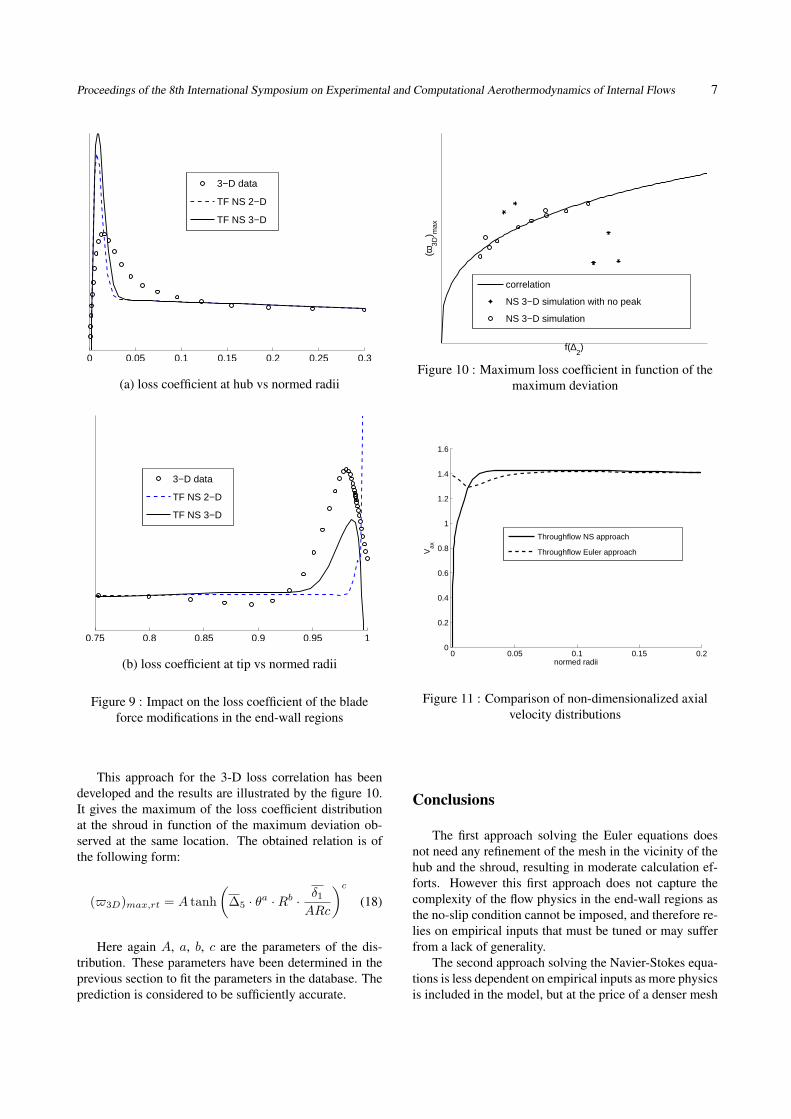
The figures 8 and 9 present the results obtained interms of deviation and loss coefficient distributions. Forboth quantities, two calculations are presented: one withthe blade force modification (TF NS 3-D) and the otherone without (TF NS 2-D). These two calculations arecompared with the distribution obtained from the 3-DNavier-Stokes calculation which represents the referencesolution.

The figure 8(a) shows the deviation in the hub region.Thanks to the constant blade force through the bound-ary layer, the overturning is predicted both in locationand magnitude. At the tip, the underturning is also pre-dicted but with less precision, as shown on figure 8(b).It is globally underestimated except very close to the tipgap. A way to improve the result would be to decrease theblade force in that region instead of keeping it constant.This would be in agreement with the experimental resultsobtained by Storer and Cumpsty [10]. The improvementbrought by the modification of the blade force comparedto the 2-D solution is clearly demonstrated.

Concerning the loss coefficient, the blade force modi-fication has only a slight effect on the flow development atthe hub (figure 9(a)). Indeed the proposed modification ofthe inviscid blade force does not model the loss generatedby the interaction of the blade and the annulus end-wall.For the tip region (figure 9(b)), the situation is different,as canceling the blade force in the tip gap induces somefriction forces at the tip of the blade. The resulting losscoefficient is more similar to the one obtained by the 3-DNavier-Stokes simulation but with a lower intensity: someflow features such as the loss generated by the tip vortexflow is not modeled in the throughflow.

In conclusion, the 3-D deviation is relatively well pre-dicted by the blade force modification model. This is notthe case for the 3-D losses as the mechanisms that gener-ate those losses is not modeled (at the exception of someparts for the tip region). A way to model these losseswould be to rely on the characteristics of the captured 3-Ddeviation. Indeed, as it is (partly) the same phenomenathat are responsible for the generation of the 3-D lossesand the 3-D deviation, it should be possible to determinethe 3-D loss coefficient from the captured 3-D deviation.For example, the maximum underturning at the tip is prob-ably well correlated with the maximum loss coefficient atthe tip. This is also true for the spanwise extent of the 3-Ddeviation and 3-D losses effects.

Proceedings of the 8th International Symposium on Experimental and Computational Aerothermodynamics of Internal Flows 7

0 0.05 0.1 0.15 0.2 0.25 0.3

3−D data

TF NS 2−D

TF NS 3−D

(a) loss coefficient at hub vs normed radii

0.75 0.8 0.85 0.9 0.95 1

3−D data

TF NS 2−D

TF NS 3−D

(b) loss coefficient at tip vs normed radii

Figure 9 : Impact on the loss coefficient of the bladeforce modifications in the end-wall regions

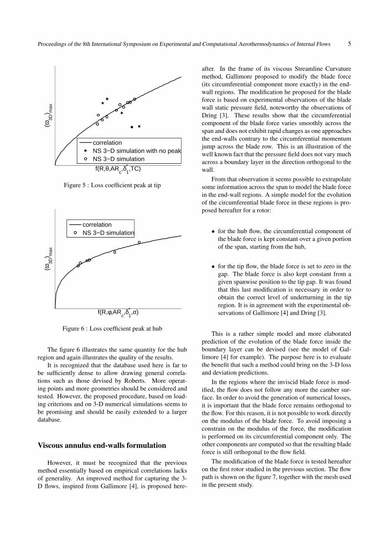
This approach for the 3-D loss correlation has beendeveloped and the results are illustrated by the figure 10.It gives the maximum of the loss coefficient distributionat the shroud in function of the maximum deviation ob-served at the same location. The obtained relation is ofthe following form:

($3D)max,rt = A tanh(

∆5 · θa ·Rb · δ1

ARc

)c

(18)

Here again A, a, b, c are the parameters of the dis-tribution. These parameters have been determined in theprevious section to fit the parameters in the database. Theprediction is considered to be sufficiently accurate.

f(∆2)

(ϖ3D

) max

correlation

NS 3−D simulation with no peak

NS 3−D simulation

Figure 10 : Maximum loss coefficient in function of themaximum deviation

0 0.05 0.1 0.15 0.20

0.2

0.4

0.6

0.8

1

1.2

1.4

1.6

normed radii

Vax

Throughflow NS approach

Throughflow Euler approach

Figure 11 : Comparison of non-dimensionalized axialvelocity distributions

Conclusions

The first approach solving the Euler equations doesnot need any refinement of the mesh in the vicinity of thehub and the shroud, resulting in moderate calculation ef-forts. However this first approach does not capture thecomplexity of the flow physics in the end-wall regions asthe no-slip condition cannot be imposed, and therefore re-lies on empirical inputs that must be tuned or may sufferfrom a lack of generality.

The second approach solving the Navier-Stokes equa-tions is less dependent on empirical inputs as more physicsis included in the model, but at the price of a denser mesh

Proceedings of the 8th International Symposium on Experimental and Computational Aerothermodynamics of Internal Flows 8

and higher computational efforts. The figure 11 showsthe improvement brought by the Navier-Stokes formula-tion over the Euler one for the radial distribution of theaxial velocity at the outlet of the first rotor. More realis-tic distributions are indeed found with the Navier-Stokesmodel.

It is believed that the combination of both approaches,i.e. the Navier-Stokes approach with captured devia-tion and 3-D losses coefficient computed through cali-brated functions (equation (18) for example) is a promis-ing way to remove a part of the empiricism included in thethroughflow model.

References

[1] S. Baralon, L.-E. Erikson and U. Hall. ViscousThroughflow Modelling of Transonic Compressors Usinga Time-Marching Finite-Volume Solver. Proceedings ofthe 13th International Symposium on Airbreathing En-gines (ISABE), Chattanooga, 1997.

[2] J.D. Denton and W.N. Dawes. Computational FluidDynamics for Turbomachinery Design. In Developmentsin Turbomachinery Design, John Denton editor, Profes-sional Engineering Publishing, 1999.

[3] R.P. Dring. Radial Transport and Momentum Ex-change in an Axial Compressor. Transactions of theASME Journal of Turbomachinery, 115:477–486, 1993.

[4] S.J. Gallimore. Viscous Throughflow Modelling ofAxial Compressor Bladerows using a Tangential Blade

Force Hypothesis. ASME Paper 97-GT-415, 1997.

[5] W.M. Konig, D.K. Hennecke, and L. Fottner. Im-proved Blade Profile Loss and Deviation Angle Modelsfor Advanced Transonic Compressor Blading : Part I - AModel for Subsonic Flow, Part II - A Model for Super-sonic Flow. Transactions of the ASME Journal of Turbo-machinery, 118:73–80, 1996.

[6] E.W. Pfitzinger and W. Reiss. A New Concept for Lossand Deviation Prediction in Throughflow Calculations ofAxial Flow Compressors. Proceedings of the 2nd Euro-pean Turbomachinery Conference, Antwerpen, 1997.

[7] W.B. Roberts, G.K. Serovy and D.M. Sandercock.Modeling the 3-D Flow Effects on Deviation Angle forAxial Compressor Middle Stages. Journal of Engineeringfor Gas Turbines and Power, 108, 1986.

[8] W.B. Roberts, G.K. Serovy and D.M. Sandercock. De-sign Point Variation of 3-D Loss and Deviation for Ax-ial Compressor Middle Stages. ASME Paper 88-GT-57,1988.

[9] J. Simon and O. Leonard. A Throughflow AnalysisTool Based on the Navier-Stokes Equations. Proceedingsof the 6th European Turbomachinery Conference, Lille,2005.

[10] J.A. Storer and N.A. Cumpsty. Tip Leakage Flow inAxial Compressors. Transactions of the ASME Journal ofTurbomachinery, 113:252, 1991.

[11] A. Sturmayr and C. Hirsch. Shock Representa-tion by Euler Throughflow Models and Comparison withPitch-Averaged Navier-Stokes Solutions. ISABE 99-7281, 1999.