9306002

8/14/2019 9306002

http://slidepdf.com/reader/full/9306002 1/49

a r X i v : h

e p - t h / 9 3 0 6 0 0 2 v 2

2 J u n 1 9 9 3

RU-93-20

BOUNDARY S-MATRIX AND BOUNDARY STATE

IN TWO-DIMENSIONAL INTEGRABLE QUANTUM FIELD THEORY

Subir Ghoshal† and Alexander Zamolodchikov ‡ ⋆

Department of Physics and AstronomyRutgers University

P.O.Box 849, Piscataway, NJ 08855-0849

Abstract

We study integrals of motion and factorizable S-matrices in two-dimensional integrablefield theory with boundary. We propose the “boundary cross-unitarity equation” which isthe boundary analog of the cross-symmetry condition of the “bulk” S-matrix. We derivethe boundary S-matrices for the Ising field theory with boundary magnetic field and forthe boundary sine-Gordon model.

1.INTRODUCTION

In this paper we study two-dimensional integrable field theory with boundary. Exact

solution to such a field theory could provide better understanding of boundary-relatedphenomena in statistical systems near criticality[1]. Quantum field theory with boundarycan be applied to study quantum systems with dissipative forces[2]. From a more generalpoint of view, studying integrable models could throw some light on the structure of the“space of boundary interactions”, the object of primary significance in open string fieldtheory[3].

An integrable field theory posesses an infinite set of mutually commutative integralsof motion1. In the “bulk theory” (i.e. without a boundary) these integrals of motionfollow from the continuity equations for an infinite set of local currents. These currentscan be shown to exist in many 2D quantum field theories, both the ones defined in terms

of an action functional (like sine-Gordon or nonlinear sigma-models[4]) and those which

† E-mail: [email protected]‡ E-mail: [email protected]⋆ Supported in part by the Department of Energy under grant No. DE–FG0590ER405591 With some reservations, this property is widely believed to be a sufficient condition.

In practice, it is usually enough to find the first few integrals of motion of spin s > 1 toargue about integrability (this argument works in all known cases).

1

http://arxiv.org/abs/hep-th/9306002v2































8/14/2019 9306002


are defined as “perturbed conformal field theories”[5]. In presence of a boundary, theexistense of these currents is not sufficient to ensure integrability. Integrals of motionappear only if particular “integrable” boundary conditions are chosen. In general, theboundary condition can be specified either through the “boundary action functional” oras the “perturbed conformal boundary condition”2. In Sect.2 we show how the integrals

of motion of the “bulk” theory get modified (in most cases destroyed) in presence of theboundary and how one can find “integrable” boundary conditions.

An important characteristic of an integrable field theory is its factorizable S-matrix.In the “bulk theory”, the factorizable S-matrix is completely determined in terms of thetwo-particle scattering amplitudes, the latter being required to satisfy the Yang-Baxterequation (also known as the “factorizability condition”), in addition to the standard equa-tions of unitarity and crossing symmetry[4]. These equations have much restrictive power,determining the S-matrix up to the so-called “CDD ambiguity”. At present many examplesof factorizable scattering theory are known (see e.g.[4,9-12]), most of which are obtained byexplicitely solving the above equations (eliminating the “CDD ambiguity” usually requiresa lot of guesswork).

It is known since long[13] that the concept of factorizable scattering can be generalizedin a rather straightforward way to the case where a reflecting boundary is present. TheS-matrix is expressed in terms of the “bulk” two-particle S-matrix and specific “boundaryreflection” amplitudes, the latter, again, being required to satisfy an appropriate gen-eralization of the Yang-Baxter equation (which we call here the “Boundary Yang-Baxterequation”) 3. Generalization of the unitarity condition is also fairly straightforward. Whatwas not known was the appropriate analog of the crossing-symmetry equation. In Section 3we fill this gap by deriving what we call the “boundary cross-unitarity equation”. Togetherwith this, the above equations have exactly the same restrictive power as the corresponding“bulk” system, i.e. they allow one to pin down the factorizable boundary S-matrix up to

the “CDD factors”.We also study integrable boundary conditions in two particular models (off-criticalIsing field theory and sine-Gordon theory) and find the associated boundary S-matrices.This is done in Sections 4 and 5.

2.INTEGRALS OF MOTIONConsider a 2D Euclidean field theory, in flat space with coordinates (x1, x2) = (x, y).

There are basically two ways to define a 2D field theory. In the Lagrangian approach onespecifies the action

A =

∞−∞

dx

∞−∞

dy a(ϕ, ∂ µϕ) (2.1)

2 Conformal field theories with boundary are studied in [6,7,8] where, in particular, it isshown how to classify conformally-invariant boundary conditions and boundary operators.

3 This equation found important applications in quantum inverse scattering method[14],generalized to the systems with boundary[15,16].

2

8/14/2019 9306002


where ϕ(x, y) is some set of “ fundamental fields” and the action density a(ϕ, ∂ µϕ) is a localfunction of these fields and derivatives ∂ µϕ = ∂ϕ/∂xµ with µ = 1, 2. Another approach isto consider the “perturbed conformal field theory”; in this case one writes the “symbolicaction”

A = ACF T + ∞−∞

Φ(x, y)dxdy (2.2)

where ACF T is the “action of conformal field theory (CFT)” and Φ(x, y) is a specificrelevant field of this CFT. In both approaches one can define a symmetric stress tensorT µν = T νµ which satisfies the continuity equations

∂ zT = ∂ zΘ ; ∂ zT = ∂ zΘ (2.3)

Here we use complex coordinates z = x + iy, z = x− iy and denote the appropriate compo-nents T = T zz , T = T zz, Θ = T zz of the stress tensor. To achieve Hamiltonian formulation

one chooses an arbitrary direction, say the y-direction, to be the “euclidean time”, and as-sociates a Hilbert space H with any “equal time section” y = const., x ∈ (−∞, ∞). Statesare vectors in H and their “time evolution” is described by the Hamiltonian operator

H =

∞−∞

dxT yy =

∞−∞

dx[T + T + 2Θ] (2.4)

Let us assume that the field theory (2.1) or (2.2) is integrable. In particular, theequations (2.3) appear to be the first representatives of an infinite sequence

∂ zT s+1 = ∂ zΘs

−1 ∂ zT s+1 = ∂ zΘs

−1 (2.5)

where T s+1, Θs−1 (T s+1, Θs−1) are local fields of spins s + 1, s − 1 respectively and theintegrals of motion (IM)

P s =

∞−∞

(T s+1 + Θs−1)dx; P s =

∞−∞

(T s+1 + Θs−1) dx (2.6)

constitute an infinite set of mutually commutative operators in H. The spin s of IM (2.6)takes integer values s1, s2,... in the infinite set {s} which is an important characteristic of an integrable field theory[5]. In any case, s1 = 1; for this value of s (2.5) coincides with(2.3) and

H = (P 1 + P 1) (2.7)

Now, let us consider this field theory in the semi-infinite plane, x ∈ (−∞, 0], y ∈(−∞, ∞), the y-axis being the boundary. Again, the boundary conditions are specifiedin different ways in the two approaches, (2.1) and (2.2). In the lagrangian approachone chooses the “boundary action density” b(ϕB(y), d

dyϕB(y)), as a local function of the

“boundary field” ϕB , ϕB(y) = ϕ(x, y)|x=0, and writes the full action in the form

3

8/14/2019 9306002


AB =

∞−∞

dy

0−∞

dxa(ϕ, ∂ µϕ) +

∞−∞

dy b(ϕB ,d

dyϕB) (2.8)

To write down the analog of (2.2) in presence of the boundary, one starts with conformalfield theory on the same semi-infinite plane with certain conformal boundary conditions(CBC) at the boundary x = 0, and defines “CBC perturbed by relevant boundary operatorΦB(y)”. In general, this perturbation of boundary condition goes along with the pertur-bation (2.2) of the bulk theory. This strategy is summarised by the symbolic “action”

A = ACFT +CBC +

∞−∞

dy

0−∞

dxΦ(x, y) +

∞−∞

dyΦB(y) (2.9)

As is argued by Cardy[6], in CFT the equation T xy|x=0 = 0 is satisfied with any choiceof CBC. In the perturbed theory (2.9) this condition is changed to

T xy|x=0 = (−i)(T −¯T )|x=0 =

d

dy θ(y) (2.10)

where θ(y) is some local boundary field. As the theory (2.8) or (2.9) is still symmetricwith respect to translations along the y-axis, the equation (2.10) can be easily derived asa consequence of this symmetry. In the “perturbed CFT” approach, it is relatively easyto relate the field θ(y) to the “boundary perturbation” ΦB(y)(see below).

The continuity equations (2.3) guarantee that the contour integrals

P 1(C) =

C

(T dz + Θdz) ; P 1(C) =

C

(T dz + Θdz) (2.11)

do not change under deformations of the integration contours

C. Consider the contour

C = C1 + C12 + C2 shown in Fig.1. Obviously, P 1(C) = P 1(C) = 0. If we take thecombination

0 = P 1(C) + P 1(C) = P 1(C 1) + P 1(C1) + P 1(C2) + P 1(C2) + P 1(C12) + P 1(C12) (2.12)

the integration over C12 part of this contour is easily done in view of (2.10)

P 1(C12) + P 1(C12) = θ(y1) − θ(y2) (2.13)

and hence the integral

H B(y) =

0−∞

(T + T + 2Θ) dx + θ(y) (2.14)

is in fact y-independent, i.e. it is an integral of motion in (2.8) or (2.9).Even if the bulk theory (2.1) or (2.2) is integrable, in general the boundary conditions

in the semi-infinite system (2.8) or (2.9) will spoil integrability. Suppose, however, thatwe can choose particular boundary conditions, such that the equation

4

8/14/2019 9306002


[T s+1 + Θs−1 − T s+1 − Θs−1]|x=0 =d

dyθs(y) (2.15)

is satisfied for some s ∈ {s}; here again θs(y) is some local boundary field. Then repeatingthe above argument, one finds that the quantity

H (s)B =

0−∞

[T s+1(x, y) + Θs−1(x, y) + T s+1(x, y) + Θs−1(x, y)] dx + θs(y) (2.16)

does not depend on y, i.e. it appears as a non-trivial integral of motion. We will callthe boundary conditions “integrable” (and refer to the theory (2.8)((2.9)) as “integrableboundary field theory”) if the equation (2.15) holds for any s out of an infinite set {s}B,subset in {s}.

There are two alternative natural ways to introduce the Hamiltonian picture in thetheory (2.8)((2.9)). First, one can take again the direction along the boundary ( y-direction)to be the “time”.In this case the boundary appears as the “boundary in space”, and theHilbert space of states HB is associated with the semi-infinite line y = const, x ∈ (−∞, 0].

Then the quantities (2.14), (2.16) appear as operators acting in HB , and H B(= H (1)B )

is naturally identified with the Hamiltonian. The correlation functions of any local fieldsOi(x, y) in presence of the boundary can be computed in this picture as the matrix elements

O1(x1, y1)...ON (xN , yN ) =B0 | T yO1(x1, y1)...ON (xN , yN ) | 0B

B0 | 0B (2.17)

where | 0B∈ HB is the ground state of H B , and Oi(xi, yi) in the r.h.s. are understood asthe corresponding Heisenburg operators

Oi(x, y) = e−yH BOi(x, 0)eyH B (2.18)

and T y means the “y-ordering”. In an integrable theory the operators H (s)B ; s ∈ {s}B,

constitute a commutative set of IMs.Alternatively, one could take x to be the “euclidean time”. In this case the “equal

time section” is the infinite line x = const, y ∈ (−∞, ∞). Hence the associated space of states is the same H as in the bulk theory (2.1)((2.2)), and the Hamiltonian operator isgiven by the same eq.(2.4) (with x and y interchanged). The boundary at x = 0 appears as

the “time boundary”, or “initial condition” at x = 0 which is described by the particular“boundary state”4| B ∈ H. It is the state | B that concentrates all information aboutthe boundary condition in this picture. The correlation functions (2.17) are expressed as

O1(x1, y1)...ON (xN , yN ) =0 | T x(O1(x1, y1)...ON (xN , yN ) | B

0 | B (2.19)

4 The notion of boundary state is discussed in the context of CFT in [7].

5

8/14/2019 9306002


where now | 0 ∈ H is the ground state of H and Oi(x, y) in the r.h.s. are the Heisenbergfield operators

Oi(x, y) = e−xH Oi(0, y)exH (2.20)

corresponding to this picture;T x means “x-ordering”. In an integrable theory, the same

equations (2.6) (again with x and y interchanged) define an infinite set of mutually com-mutative operators P s, P s; s ∈ {s}, acting in H. As a direct consequence of (2.15) one findsthat the boundary state | B satisfies the equations

(P s − P s) | B = 0 ; s ∈ {s}B. (2.21)

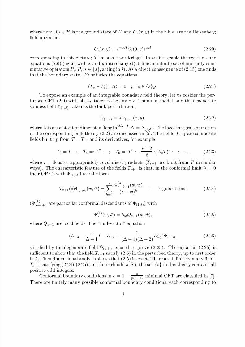
To expose an example of an integrable boundary field theory, let us cosider the per-turbed CFT (2.9) with ACF T taken to be any c < 1 minimal model, and the degeneratespinless field Φ(1,3) taken as the bulk perturbation,

Φ(x,y) = λΦ(1,3)(x, y). (2.22)

where λ is a constant of dimension [length]2∆−2; ∆ = ∆(1,3). The local integrals of motionin the corresponding bulk theory (2.2) are discussed in [5]. The fields T s+1 are compositefields built up from T = T zz and its derivatives, for example

T 2 = T ; T 4 =: T 2 : ; T 6 =: T 3 : −c + 2

6: (∂ zT )2 : ; ... (2.23)

where : : denotes appropriately regularized products (T s+1 are built from T in similarways). The characteristic feature of the fields T s+1 is that, in the conformal limit λ = 0their OPE’s with Φ(1,3) have the form

T s+1(z)Φ(1,3)(w, w) =s

k=1

Ψ(k)s−k+1(w, w)

(z − w)k+ regular terms (2.24)

(Ψ(k)s−k+1 are particular conformal descendants of Φ(1,3)) with

Ψ(1)s (w, w) = ∂ wQs−1(w, w), (2.25)

where Qs−1 are local fields. The “null-vector” equation

(L−3 − 2

∆ + 1L−1L−2 +

1

(∆ + 1)(∆ + 2)L3−1)Φ(1,3), (2.26)

satisfied by the degenerate field Φ(1,3), is used to prove (2.25). The equation (2.25) issufficient to show that the field T s+1 satisfy (2.5) in the perturbed theory, up to first orderin λ. Then dimensional analysis shows that (2.5) is exact. There are infinitely many fieldsT s+1 satisfying (2.24)-(2.25), one for each odd s. So, the set {s} in this theory contains allpositive odd integers.

Conformal boundary conditions in c = 1 − 6 p( p+1) minimal CFT are classified in [7].

There are finitely many possible conformal boundary conditions, each corresponding to

6

8/14/2019 9306002


a particular cell (r, s) of the Kac table. In each case possible boundary operators aredegenerate primary boundary fields ψ(n,m) (plus their Virasoro descendants), such that

the fusion rule coefficients N (r,s)(n,m)(r,s) are non-zero (the other degenerate boundary fields,

with N (r,s)(n,m)(r,s) = 0 correspond to “juxtapositions” of different conformal boundaries, see

[7] for details). The field Φ(1,3) satisfies this condition for any (r, s). We take this field tobe the boundary perturbation in (2.9), i.e.

ΦB(y) = λBψ(1,3)(y). (2.27)

Its conformal dimension ∆ = ∆(1,3) < 1, so that it is a relevant perturbation. We want toshow that under this choice the theory (2.9) is integrable.

To warm up, let us consider the components T and T of the stress tensor itself. Inthe conformal limit λ = 0, λB = 0, these components satisfy the boundary condition

[T (y + ix) − T (y − ix)]|x=0 = 0, (2.28)

i.e. the field T (z) is just the analytic continuation of T (z) to the lower half-plane Imz < 0.Let us “turn on” the boundary perturbation, λB=0, still keeping λ = 0, and consider thecorrelation function

[T (y + ix) − T (y − ix)]X λB =

Z −1λB[T (y + ix) − T (y − ix)]Xe

−λB ∞

−∞

ψ(1,3)(y′)dy′CF T , (2.29)

where X is any product of fields located away from the boundary x = 0 and Z −1λB=

e−λB

∞

−∞

ψ(1,3)(y)dyCF T . In the limit x → 0 the contribution to (2.29) is controlled by

OPE

(T (y + ix) − T (y − ix))λBψ(1,3)(y′) =

λB{ ∆(1,3)

(y − y′ + ix)2− ∆(1,3)

(y − y′ − ix)+

1

(y − y′ + ix)

∂

∂y ′− 1

(y − y′ − ix)

∂

∂y ′}ψ(1,3)(y′) →

→ λB{∆(1,3)δ′(y − y′) + δ(y − y′)∂

∂y ′}ψ(1,3)(y′). (2.30)

This shows that for λB = 0 the fields T (x, y) and T (x, y) satisfy (2.10) with

θ(y) = (1 − ∆)λBψ(1,3)(y). (2.31)

Now, dimensional analysis, exactly parallel to that carried out in [5] shows that the equa-tions (2.10),(2.30) remain valid if we turn on the bulk perturbation, i.e. at λ = 0.

The above arguments can be repeated for the higher currents T s+1, s = 3, 5,.... To seethis, note that the null vector equation (2.26), crucial for the validity of (2.25), is satisfiedby ψ(1,3) as well. Therefore, in the conformal limit λ = λB = 0 the fields T s+1(z) satisfythe OPEs

7

8/14/2019 9306002


T s+1(z)ψ(1,3)(y) =

sk=1

1

(z − y)kχ(k)s+1−k(y) + regular terms,

χ(1)s (y) =

d

dyqs(y), (2.32)

similar to (2.24),(2.25) where qs, χ are descendants of ψ(1,3). Whence

limitx→0(T s+1(y + ix) − T s+1(y − ix)) λBψ(1,3)(y′)

= λB(δ(y − y′)d

dy′qs(y′) +

sk=2

1

(k − 1)!

dk−1

dy′k−1δ(y − y′)χk

s+1−k(y′)), (2.33)

and we conclude that for λ = 0 and in the first order in λB the equation holds

[T s+1(x, y) − T s+1(x, y)]x=0 =

d

dy θs (2.34)

with

θs(y) = λB[qs(y) +

sk=2

1

(k − 1)!

dk−1

dyk−1χks+1−k(y)]. (2.35)

The higher powers of λB can contribute to (2.34) through the “resonance terms” similarto those discussed in [5]. It is plausible, however,that these do not spoil the general formof (2.34) but simply modify (2.35) by higher order terms in λB . It is also plausible (andcan be supported to some extent by dimensional analysis of [5]) that “turning on” the bulk

perturbation, λ = 0, converts (2.34) to(2.15).We realise that the above arguments do not constitute a rigorous proof. First, we

did not solve the problem of the “resonance terms” (this problem remains open in thebulk theory, too). More importantly, we did not analyse possible effects of mixing betweenthe boundary and the bulk perturbations. We have shown,however,that the field theory(2.9) with (2.22) and (2.26) satisfies some very non-trivial necessary (but not sufficient)conditions of integrability and we conjecture that this boundary field theory with boundaryis integrable.

3.BOUNDARY S-MATRIXIf the field theory (2.1) ((2.2)) is massive the space H is the Fock space of multiparticle

states. After rotation y = it to 1 + 1 Minkowski space-time these states are interpretedas the asymptotic (“in-” or “out-”) scattering states. For an integrable field theory thescattering is purely elastic and the corresponding S-matrix is factorizable. The factorizablescattering theory in infinite space is discussed in many papers and reviews (see e.g.[4,5,9-12]); below, we describe just some basics of the theory. The boundary theory (2.8)((2.9))in Minkowski space is also interpreted as a scattering theory. For the integrable boundary

8

8/14/2019 9306002


field theory this scattering theory is again purely elastic and the corresponding S-matrixis the “factorizable boundary S-matrix”. The “factorizable boundary scattering theory”is developed in close parallel with the “bulk” theory (see [13]). However there are stillsome gaps in this parallel (most importantly, the boundary analog of crossing-symmetrycondition of the “bulk” S-matrix is not absolutely straightforward). It is the aim of this

Section to fill these gaps.We start with a brief description of the basics of the factorizable scattering theory in

the infinite space (“bulk theory”). Assume that the theory contains n sorts of particlesAa; a = 1, 2,...,n with the masses ma. As usual, we describe the kinematic states of theparticles in terms of their rapidities θ,

p0 + p1 = meθ; p0 − p1 = me−θ, (3.1)

where pµ are the components of the two-momentum and m is the particle mass. Theasymtotic particle states are generated by the “particle creation operators” Aa(θ)

| Aa1(θ1)Aa2(θ2)...AaN (θN ) = Aa1(θ1)Aa2(θ2)...AaN (θN ) | 0. (3.2)

The state (3.2) is interpreted as an “in-state” if the rapidities θi are ordered as θ1 > θ2 >... > θN ; if instead θ1 < θ2 < ... < θN (3.2) is understood as an “out-state” of scattering.The “creation operators” Aa(θ) satisfy the commutation relations

Aa1(θ1)Aa2(θ2) = S b1b2a1a2(θ1 − θ2)Ab2(θ2)Ab1(θ1) (3.3)

which are used to relate the “in-” and the “out-” bases and hence completely describe theS-matrix. The coefficient functions S b1b2a1a2(θ) are interpreted as the two-particle scatteringamplitudes describing the processes Aa1Aa2 → Ab1Ab2 (see Fig.2). The asymptotic states(3.2) diagonalise the local IM (2.6), the eigenvalues being determined by the relations

[P s, Aa(θ)] = γ (s)a esθAa(θ); [P s, Aa(θ)] = γ (s)a e−sθAa(θ); (3.4)

P s | 0 = 0; P s | 0 = 0, (3.5)

where γ (s)a are constants (γ

(1)a = ma). These IM must commute with the S-matrix; it

follows in particular that the amplitude S b1b2a1a2(θ) is zero unless ma1 = mb1 and ma2 = mb2

(other concequences are discussed in [5]).Charge conjugation C acts as an involution of the set of particles {Aa}, i.e. C : Aa ↔

Aa, where Aa

∈{Aa

}, so that each particle in

{Aa

}is either neutral CAa = Aa or belongs

to the particle-antiparticle pair (Aa, Aa). In this Section we assume for simplicity that thetheory under consideration respects C, P and T symmetries, i.e.

S b1b2a1a2(θ) = S b1b2a1a2(θ) = S b2b1a2a1(θ) = S a2a1b2b1

(θ). (3.6)

The two-particle S-matrix S b1b2a1a2(θ) is the basic object of the theory. It must satisfyseveral general requirements

1.Yang-Baxter (or “factorization”) equation

9

8/14/2019 9306002


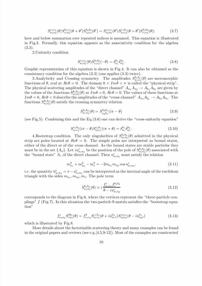
S c1c2a1a2(θ)S b1c3c1a3(θ + θ′)S b2b3c2c3 (θ′) = S c2c3a2a3(θ′)S c1b3a1c3(θ + θ′)S b1b2c1c2 (θ); (3.7)

here and below summation over repeated indices is assumed. This equation is illustratedin Fig.3. Formally, this equation appears as the associativity condition for the algebra(3.3).

2.Unitarity condition

S c1c2a1a2(θ)S b1b2c1c2 (−θ) = δb1a1δb2a2 . (3.8)

Graphic representation of this equation is shown in Fig.4. It can also be obtained as theconsistancy condition for the algebra (3.3) (one applies (3.3) twice).

3.Analyticity and Crossing symmetry. The amplitudes S b1b2a1a2(θ) are meromorphicfunctions of θ, real at Reθ = 0. The domain 0 < Imθ < π is called the “physical strip”.The physical scattering amplitudes of the “direct channel” Aa1Aa2 → Ab1Ab2 are given bythe values of the functions S b1b2a1a2(θ) at Imθ = 0, Reθ > 0. The values of these functions atImθ = 0, Reθ < 0 describe the amplitudes of the “cross-channel” Aa2Ab

1 →Ab2Aa1 . The

functions S b1b2a1a2(θ) satisfy the crossing symmetry relation

S b1b2a1a2(θ) = S b2a1a2 b1

(iπ − θ) (3.9)

(see Fig.5). Combining this and the Eq.(3.8) one can derive the “cross-unitarity equation”

S c1b2a1c2(iπ − θ)S c2b1a2c1(iπ + θ) = δb1a1δb2a2 . (3.10)

4.Bootstrap condition. The only singularities of S b1b2a1a2(θ) admitted in the physicalstrip are poles located at Reθ = 0. The simple poles are interpreted as bound states,either of the direct or of the cross channel. As the bound states are stable particles they

must be in the set {Aa}. Let iuca1a2 be the position of the pole of S b1b2a1a2(θ) associated withthe “bound state” Ac of the direct channel. Then uca1a2 must satisfy the relation

m2a1 + m2

a2− m2

c = −2ma1ma2 cos uca1a2 , (3.11)

i.e. the quantity uca1a2 = π −uca1a2 can be interpreted as the internal angle of the euclideantriangle with the sides ma1 , ma2 , mc. The pole term

S b1b2a1a2(θ) ≃ if ca1a2f b1b2c

θ − iuca1a2(3.12)

corresponds to the diagram in Fig.6, where the vertices represent the “three-particle cou-

plings” f (Fig.7). In this situation the two-particle S-matrix satisfies the “bootstrap equa-tion”

f ca1a2S bb3ca3(θ) = f bc1c2S c1b3a1c3(θ + iua2a1c)S c2c3a2a3(θ − iua1a2c) (3.13)

which is illustrated by Fig.8.More details about the factorizable scattering theory and many examples can be found

in the original papers and reviews (see e.g.[4,5,9-12]). Most of the examples are constructed

10

8/14/2019 9306002


directly, by solving the Eq.(3.7-3.9) above. Following this approach one can pin down theS-matrix S b1b2a1a2(θ) up to the so-called “CDD ambiguity”

S b1b2a1a2(θ) → S b1b2a1a2

(θ)Φ(θ), (3.14)

where the “CDD factor” Φ(θ) is an arbitrary function satisfying the equations

Φ(θ) = Φ(iπ − θ); Φ(θ)Φ(−θ) = 1. (3.15)

The bootstrap equation may impose further restrictions on this function.Let us turn now to the semi-infinite system (2.8)((2.9)). Here again the states in HB

can be classified as asymptotic scattering states. The scattering occurs in the semi-infinite1 + 1 Minkowski space-time (x, t), t = −iy, x < 0. The initial state

| Aa1(θ1)Aa2(θ2)...AaN (θN )B,in (3.16)

(the subscript B indicates that

|...

B

∈ HB) of the scattering consists of some number

(N ) of “incoming” particles moving towards the boundary at x = 0, i.e. all the rapiditiesθ1, θ2,...,θN are positive. In the infinite future, t → ∞, this state becomes a superpositionof the “out-states”

| Ab1(θ1′)Ab2(θ2

′)...AbM (θM ′)B,out (3.17)

each containing some number of “outgoing” particles moving away from the boundarywith negative rapidities θ1

′, θ2′,...,θM

′. In integrable boundary field theory this process isconstrained by the IM (2.16). Like in the “bulk” theory the operators H s are diagonal inthe basis of asymptotic states and

H s | Aa1(θ1)Aa2(θ2)...AaN (θN )B,in(out) =

(N i=1

2γ (s)ai cosh(sθi) + h(s)) | Aa1(θ1)Aa2(θ2)...AaN (θN )B,in(out) (3.18)

where h(s) are some constants. The constraints

N i=1

γ (s)ai cosh(sθi) =M j=1

γ (s)bj

cosh(sθj′) (3.19)

which follow from (3.18) show that M = N and the set of rapidities {θ1′, θ2′,...,θN ′} candiffer only by permutation from {−θ1, −θ2, ...,−θN }, i.e. the boundary scattering theoryis purely elastic. It is possible to argue that the S-matrix in this case has a factorizablestructure.

The factorizable boundary scattering theory can be described in complete analogywith the “bulk” scattering theory. Again, the asymptotic states (3.16),(3.17) are generatedby the “creation operators” Aa(θ) satisfying the same commutation relations (3.3). If θ1 > θ2 > ... > θN > 0 the in-state (3.16) can be written as

11

8/14/2019 9306002


Aa1(θ1)Aa2(θ2)...AaN (θN ) | 0B, (3.20)

where | 0B is the ground state of H B. One can think of the boundary as an infinitelyheavy impenetrable particle B sitting at x = 0 and formally write the state | 0B as

| 0B = B | 0 (3.21)

in terms of “operator” B which we call the “boundary creating operator”(formally B :H → HB ; it is an interesting question wether (3.21) makes any more than just formalsense). The “operator” B satisfies the relations

Aa(θ)B = Rba(θ)Ab(−θ)B, (3.22)

the coefficient functions Rba(θ) being interpreted as the amplitudes of one-particle reflection

off the boundary, as shown in Fig.9. The Eq.(3.18) is reproduced if we assume (3.4), (3.5)and [H

s, B] = h(s)B. It follows from (3.17) that Rb

a(θ) vanishes if m

a = m

b. By purely

algebraic manipulations, with the use of relations (3.3) and (3.22), one can expand anyin-state (3.20) in terms of the out-states

Ab1(−θ1)Ab2(−θ2)...AbN (−θN ) | 0B, (3.23)

(θ1 > θ2 > ... > θN > 0) thus expressing the N -particle S-matrix

Aa1(θ1)Aa2(θ2)...AaN (θN ) | 0B =

Rb1b2...bNa1a2...aN (θ1, θ2,...,θN )Ab1(−θ1)Ab2(−θ2)...AbN (−θN ) | 0B (3.24)

in terms of the “fundamental amplitudes” S b1b2a1a2(θ) and Rba(θ) which are basic objects of the factorizable boundary scattering theory. The amplitudes Rb

a(θ) have to satisfy severalgeneral requirements analogous to the requirements 1 − 4 of the “bulk” theory above.

1′.Boundary Yang-Baxter equation

Rc2a2(θ2)S c1d2a1c2 (θ1 + θ2)Rd1

c1 (θ1)S b2b1d2d1(θ1 − θ2) =

S c1c2a1a2(θ1 − θ2)Rd1c1 (θ1)S d2b1c2d1

(θ1 + θ2)Rb2d2

(θ2) (3.25)

(represented graphically in Fig.10) can be obtained as the associativiy condition of the alge-bra (3.22), (3.3). These equations have been introduced first in [13] and studied in relation

with the quantum inverse scattering method for the integrable systems with boundary inmany subsequent papers (see e.g. [15-17]). Note that (3.25) is the direct analog of (3.7).

2′.Boundary Unitarity condition

Rca(θ)Rb

c(−θ) = δba (3.26)

is also an absolutely straightforward generalization of (3.8) (see Fig.11). One obtains (3.26)applying (3.22) twice.

12

8/14/2019 9306002


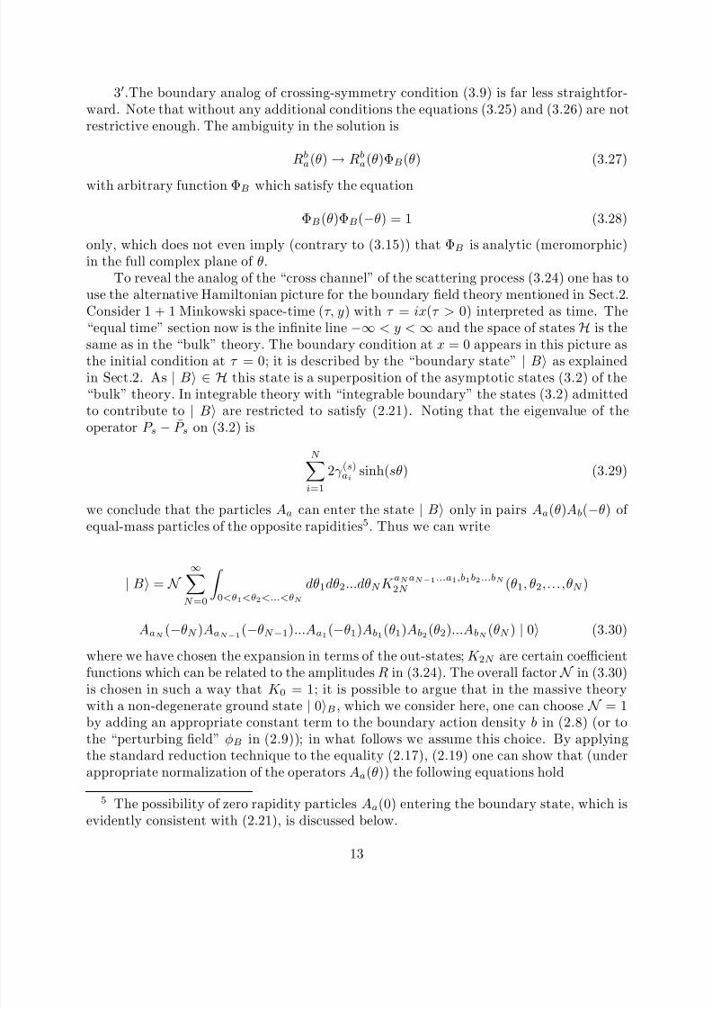
3′.The boundary analog of crossing-symmetry condition (3.9) is far less straightfor-ward. Note that without any additional conditions the equations (3.25) and (3.26) are notrestrictive enough. The ambiguity in the solution is

Rba(θ)

→Rba(θ)ΦB(θ) (3.27)

with arbitrary function ΦB which satisfy the equation

ΦB(θ)ΦB(−θ) = 1 (3.28)

only, which does not even imply (contrary to (3.15)) that ΦB is analytic (meromorphic)in the full complex plane of θ.

To reveal the analog of the “cross channel” of the scattering process (3.24) one has touse the alternative Hamiltonian picture for the boundary field theory mentioned in Sect.2.Consider 1 + 1 Minkowski space-time (τ, y) with τ = ix(τ > 0) interpreted as time. The“equal time” section now is the infinite line −∞ < y < ∞ and the space of states H is thesame as in the “bulk” theory. The boundary condition at x = 0 appears in this picture asthe initial condition at τ = 0; it is described by the “boundary state” | B as explainedin Sect.2. As | B ∈ H this state is a superposition of the asymptotic states (3.2) of the“bulk” theory. In integrable theory with “integrable boundary” the states (3.2) admittedto contribute to | B are restricted to satisfy (2.21). Noting that the eigenvalue of theoperator P s − P s on (3.2) is

N i=1

2γ (s)ai sinh(sθ) (3.29)

we conclude that the particles Aa can enter the state | B only in pairs Aa(θ)Ab(−θ) of

equal-mass particles of the opposite rapidities5

. Thus we can write

| B = N ∞

N =0

0<θ1<θ2<...<θN

dθ1dθ2...dθN K aNaN−1...a1,b1b2...bN2N (θ1, θ2,...,θN )

AaN (−θN )AaN−1(−θN −1)...Aa1(−θ1)Ab1(θ1)Ab2(θ2)...AbN (θN ) | 0 (3.30)

where we have chosen the expansion in terms of the out-states; K 2N are certain coefficientfunctions which can be related to the amplitudes R in (3.24). The overall factor N in (3.30)is chosen in such a way that K 0 = 1; it is possible to argue that in the massive theory

with a non-degenerate ground state | 0B , which we consider here, one can choose N = 1by adding an appropriate constant term to the boundary action density b in (2.8) (or tothe “perturbing field” φB in (2.9)); in what follows we assume this choice. By applyingthe standard reduction technique to the equality (2.17), (2.19) one can show that (underappropriate normalization of the operators Aa(θ)) the following equations hold

5 The possibility of zero rapidity particles Aa(0) entering the boundary state, which isevidently consistent with (2.21), is discussed below.

13

8/14/2019 9306002


K aNaN−1...a1,b1b2...bN (θ1, θ2,...,θN ) = Rb1b2...bNa1a2...aN (

iπ

2− θ1,

iπ

2− θ2, ...,

iπ

2− θN ), (3.31)

up to a constant phase factor which depends on the normalizations of the operators Aa(θ);

in what follows we assume that they are normalized in such a way that (3.31) holds as itstands.

Let us concentrate attention on the amplitude K ab(θ) ≡ K a,b2 (θ) describing the con-tribution

| B = (1 +

∞0

K ab(θ)Aa(−θ)Ab(θ) + ...) | 0 (3.32)

of the two-particle out-state Aa(−θ)Ab(θ) | 0 to the boundary state | B. It satisfies

K ab(θ) = Rba(

iπ

2− θ) (3.33)

i.e. the “elementary reflection amplitude”Rba(θ) can be obtained by analytic continuation of

the amplitude K ab(θ) to the domain Imθ = iπ2 , Reθ < 0. The values of K ab(θ) at negative

real θ (corresponding to the “lower edge” of the cut in the energy plane) are interpretedas the coefficients of expansion of | B in terms of the in−states Aa(θ)Ab(−θ) | 0, θ > 0

| B = (1 +

∞0

K ab(−θ)Aa(θ)Ab(−θ) + ...) | 0 (3.34)

As the in− and the out− states are related through the S-matrix, the amplitude K ab(θ)has to satisfy the following “boundary cross-unitarity condition”

K ab(θ) = S aba′b′(2θ)K b′a′(−θ) (3.35)

which we consider to be the boundary analog of (3.10). It is illustrated by the diagramin Fig.12. With this equation added, the ambiguity in the solution of (3.25), (3.26) and(3.35) reduces to (3.27) with ΦB satisfying (3.28) and

ΦB(θ) = ΦB(iπ − θ) (3.36)

which is exactly the same as the “CDD umbiguity” (3.14), (3.15) in the “bulk” theory.Let us note that (3.35) allows one to write (3.32) as

| B = (1 +1

2 ∞−∞ K ab(θ)Aa(−θ)Ab(θ) + ...) | 0 (3.37)

Using the Equation (3.31) one can express all the amplitudes K 2N in (3.30) in terms of the two-particle boundary amplitudes K ab(θ) and the elements of the two-particle S-matrixS cdab(θ). The result is in exact agreement with the following simple expression

| B = Ψ[K (θ)] | 0 = exp(

∞−∞

dθK (θ)) | 0 (3.38)

14

8/14/2019 9306002


where

K (θ) =1

2K ab(θ)Aa(−θ)Ab(θ) (3.39)

Note that although the “creation operators” Aa(θ) do not comute, the bilinear expressions

(3.39) satisfy the commutativity conditions

[K (θ), K (θ′)] = 0 (3.39)

as a direct consequence of the “boundary Yang-Baxter equation” (3.25) and (3.33); there-fore there is no ordering problem in (3.38). The commutativity (3.39) is crucial for theinterpretation of Ψ in (3.38) as the “wave function” of the boundary state.

The “crossing equations” (3.33), (3.35) and the expression (3.38) for the boundarystate are the main results of this Section. We feel that the simple universal form (3.38) of the boundary state is not accidental. However at the moment we do not have a satisfactoryunderstanding of its profound meaning and we can not offer anything better than the direct

derivation through (3.31).4′.Now we turn to the “boundary bootstrap conditions”. There are two sorts of these:the bootstrap conditions describing the boundary scattering of the “bound-state” particlesand the conditions related to possible existence of the “boundary bound states”.

If the particle Ac can be interpreted as the bound state of AaAb (i.e. the pole at θ =iucab, with ucab satisfying (3.11)), the boundary S-matrix elements Rd

c(θ) can be obtainedby taking the appropriate residue in the bound-state pole of the two-particle boundaryS-matrix Rab

ab(θ1, θ2). This way one gets the equation

f abd Rdc(θ) = f b1a1c Ra2

a1(θ + iubad)S b2ab1a2(2θ + iubad − iuabd)Rb

b2(θ − iuabd) (3.40)

(u ≡ iπ − u) which has the diagrammatic representation shown in Fig.13. If the particlesAa and Ab have equal masses one can expect the appearence of a pole of Rb

a(θ) at θ =iπ2

− ucab2 = ucab − iπ

2 due to the diagram in Fig.14. The corresponding residue can bewritten as

K ab(θ) ≃ i

2

f abc gc

θ − iucab, (3.41)

where the “three-particle couplings” f are the same as in (3.12) but gc are new constantsdescribing the “couplings” of the particles Ac to the boundary (Fig.14). More precisely, the

nonzero value of g

c

indicates that the boundary state | B contains a separate contributionof the zero-momentum particle Ac, i.e.

| B = N (1 + gcAc(0) +1

2

∞−∞

dθK ab(θ)Aa(−θ)Ab(θ) + ...) | 0. (3.42)

Let us stress again that in our previous analysis of the boundary state we have ignoredthis possibility, i.e. strictly speaking validity of the equation (3.38) above is limited to thecase when gc = 0 for all the particles Ac in the theory. It is easy to show that

15

8/14/2019 9306002


[gcAc(0), K (θ)] = 0, (3.43)

where K (θ) is the bilinear operator (3.39), and so in the general case one can look forthe “boundary wave function” in the form Ψ[gcAc(0), K (θ)]. The commutativity (3.43)follows from the relation

gc′

K a′b(θ)S cac′a′(θ) = gc

′

K ab′

(θ)S cbb′c′(θ) (3.44)

(Fig.15) which is easily obtained if one considers the limit θ → iπ2

− 12uca1b1 in (3.25) and

takes into account (3.13). It is also possible to show that if gc1, gc2 = 0 the amplitudeK c1c2(θ) has the pole at θ = 0 with the residue

K c1c2(θ) ≃ − i

2

gc1gc2

θ; (3.45)

This pole term is illustrated by the diagram in Fig.16.Let us illustrate these bootstrap conditions with an example of the so-called “Lie-

Yang field theory”. This field theory describes the scaling limit of Ising Model with purelyimaginary external field, the critical point being the “Lie-Yang edge singularity”(see [18]).It is a massive field theory which can be obtained by perturbing the c = −22

5 minimalCFT by its only nontrivial primary field ϕ ≡ Φ(1,2), which has a conformal dimension

∆ = −15

. Mussardo and Cardy[11] have shown that the “bulk” theory is integrable; theyhave also found the corresponding factorizable “bulk” S-matrix. The theory contains onlyone species of particles, A, and the “bulk” S-matrix is described by

A(θ1)A(θ2) = S (θ1 − θ2)A(θ2)A(θ1) (3.46)

with

S (θ) =sinh θ + i sin 2π

3

sinh θ − i sin 2π3

. (3.47)

The pole of S (θ) at θ = 2πi3 ( which has negative residue thus making non-unitarity of this

theory manifest) corresponds to the same particle A appearing as the “AA bound state”.Here we do not attempt to analyze the possible integrable boundary conditions in thistheory; we just assume that such ones do exist. Then the factorizable boundary S-matrixis described by (3.46) and

A(θ)B = R(θ)A(

−θ)B, (3.48)

where the boundary scattering amplitude R has to satisfy (3.26) and (3.35) (the boundaryYang-Baxter equation (3.25) is satisfied identically), i.e.

R(θ)R(−θ) = 1; K (θ) = S (2θ)K (−θ); K (θ) = R(iπ

2− θ). (3.49)

As the particle A appears as the “bound state”, the equation (3.40) has to be imposed aswell,

16

8/14/2019 9306002


R(θ) = S (2θ)R(θ +iπ

3)R(θ − iπ

3). (3.50)

There are two “minimal” solutions to (3.49), (3.50)6,

R(1)(θ) = −sinh(θ2 +

iπ4 )

sinh(θ2 − iπ4 )

sinh(θ2 +

iπ12 )

sinh(θ2 − iπ12 )

sinh(θ2 −

iπ3 )

sinh(θ2 + iπ3 )

, (3.51)

R(2)(θ) =sinh( θ2 − iπ

4 )

sinh( θ2 + iπ4 )

sinh(θ2 − 5iπ12 )

sinh(θ2 + 5iπ12 )

sinh( θ2 − iπ3 )

sinh( θ2 + iπ3 )

(3.52)

(of course R(1) and R(2) are related through the “CDD factor” (3.27)). These two solutions

have rather different physical properties. R(1)(θ) exhibits a pole at θ = iπ6 associated with

the diagram in Fig.14. This means that for this solution the boundary state | B(1) containsthe single-particle contribution

| B(1) = (1 + g(1)A(0) + ...) | 0 (3.53)with non-zero amplitude g(1). Explicit calculation gives

g(1) = 2i

2√

3 − 3. (3.54)

Accordingly, the amplitude R(1)(θ) has a pole at θ = iπ2 with the residue

R(1)(θ) ≃ ig2(1)2θ − iπ

. (3.55)

The solution R(2) does not have any poles in the physical strip, i.e. g(2) = 0.

In the general case the poles (3.41) and (3.45) do not exhaust all possible singularitiesthe amplitudes Rb

a(θ) may have in the “physical strip” 0 ≤ Imθ ≤ π. Even with givenboundary action (2.8)((2.9)) the boundary can exist in several stable states | αB; α =0, 1,...,nB−1 (let us stress that all these states belong to HB). These states are eigenstatesof the operators (2.16)

H s | αB = h(s)α | αB , (3.56)

with some eigenvalues h(s)α ; in particular eα = h

(1)α is the energy of the state | αB. We

assume that e0 is the smallest of eα, i.e. as before the state | 0B is the ground state of H B

7. If eα

−e0 < min ma the state

|α

B is stable just because its decay is forbidden

energetically; higher IM H s could ensure stability of | αB even if eα − e0 > min ma. Inany case, the states | αB must show up as the virtual states in the boundary scatteringprocesses. The amplitudes Rb

a(θ) can exhibit the poles

6 We call “minimal” the solution which has “minimal” set of zeroes and poles in thephysical strip 0 ≤ Imθ ≤ π, i.e. one can not reduce the total number of zeroes and polesin this strip without violating (3.49), (3.50).

7 Here we assume that the ground state is not degenerate.

17

8/14/2019 9306002


Rba(θ) ≃ i

2

gαa0gb0αθ − ivα0a

, (3.57)

where gαa0 are “boundary-particle couplings” and vα0a satisfy

e0 + ma cos(vα0a) = eα, (3.58)

see Fig.17. Thus the states | αB with eα > e0 can be interpreted as the “boundary boundstates”, eα − e0 being the binding energy.

In this situation it is natural to generalize (3.22) to

Aa(θ)Bα = Rbβaα(θ)Ab(−θ)Bβ, (3.59)

where Bα are formal “boundary creating operators” analogous to (3.21) and Rbβaα(θ) are

amplitudes of the scattering process involving the change of the state of boundary, asshown in Fig.18. Again, the amplitude Rbβ

aα(θ) does not vanish only if ma = mb and

eα = eβ , as it follows from (3.56). The equations (3.25), (3.26), (3.33), (3.35), (3.40) abovecan be generalized in an obvious way to include these amplitudes. Here we quote only the“boundary bound state bootstrap equation”

gγaαRb′βbγ (θ) = gβa2γS b1a1ba (θ − ivβaα)Rb2γ

b1α(θ)S a2b

′

a1b2(θ + ivβaα) (3.60)

shown in Fig.19; here the parameter vβaα satisfies the equation

eα + ma cos(vβaα) = eβ , (3.61)

analogous to (3.38), and gβaα are the “particle-boundary coupling constants” (Fig.20) en-

tering the residues

Rbβaα(θ) ≃ i

2

gγaαgbβγθ − ivγaα

. (3.62)

Note that (3.44) and (3.45) can be considered as particular cases α = β = γ = 0 of (3.60)and (3.62), resp., if we think of the ground state | 0B as the “bound state” of some particleAc (with gc = 0) and itself.

We have implicitely assumed in the above discussion that the ground state | 0B isnon-degenerate. This assumption is taken for the sake of simplicity only; it is not nesessaryeither from a physical point of view or for mathematical consistency. It is straightforwardto incorporate the possibility of degenerate ground states into the above picture. In thenext two Sections, where we consider examples of the factorizable boundary scatteringtheory, we will encounter this interesting possibility.

4.ISING MODEL.As is known, the scaling limit of the Ising Model with zero external field is described

by the free Majorana fermion field theory

18

8/14/2019 9306002


A =

dydx aFF (ψ, ψ), (4.1)

where

aFF (ψ, ψ) = ψ∂ zψ − ψ∂ zψ + mψψ. (4.2)

Here (z, z) are complex coordinates and m ≃ T c − T . The field theories correspondingto the high-temperature (T − T c → 0+) and the low temperature (T − T c → 0−) phasesof the Ising Model are equivalent (they are related through the duality transformationψ → ψ; ψ → −ψ, which changes the sign of m in (4.1)). Here we will assume that m > 0and interpret this field theory as the low-temperature phase. In this phase there are twodegenerate ground states, | 0, ±, so that the corresponding expectation values of the spin

field σ(x) are σ(x)± = ±σ, where σ ∼ m18 is the spontaneous magnetization.

The bulk theory (4.1) contains one sort of particles - the free fermion A with the massm. Intuitively, this particle can be understood as a “kink” (or “domain wall”) separating

domains of opposite magnetization. The corresponding particle creation operator A†(θ)(we denote it here A† to comply with the conventional notations) can be defined throughthe decomposition

ψ(x, t) =

∞−∞

dθ[ωeθ2 A(θ)eimx sinh θ+imt cosh θ + ωe

θ2 A†(θ)e−imx sinh θ−imt cosh θ];

ψ(x, t) =

∞

−∞

dθ[ωe−θ2 A(θ)eimx sinh θ+imt cosh θ + ωe−

θ2 A†(θ)e−imx sinh θ−imt cosh θ], (4.3)

where t = iy and ω = exp( iπ4 ); ω = exp(− iπ4 ). The operators A(θ), A†(θ) satisfy canoni-

cal anticommutation relations {A(θ), A†(θ′)} = δ(θ − θ′); {A(θ), A(θ′)} = {A†(θ), A†(θ′)}= 0. The last of these relations,

A†(θ)A†(θ′) = −A†(θ′)A†(θ), (4.4)

has the same meaning as (3.3) so that the free-fermion two particle S-matrix is [19]

S = −1. (4.5)

Let us consider now this field theory in the half-plane x < 0, with the boundary at

x = 0. Assuming that the boundary conditions are chosen to be integrable, we can definethe boundary scattering amplitude R(θ),

A†(θ)B = R(θ)A†(−θ)B. (4.6)

As is discussed in Sect.3, this amplitude has to satisfy (3.26), (3.33), (3.35), i.e.

R(θ)R(−θ) = 1; K (θ) = −K (−θ);

19

8/14/2019 9306002


K (θ) = R(iπ

2− θ). (4.7)

We consider first two simplest boundary conditions - the “free” and the “fixed” ones 8.a). “Fixed” boundary condition. In the microscopic theory this boundary condition

corresponds to fixing the boundary spins to be, say, +1. Obviously, this boundary condition

removes the ground state degeneracy. In terms of the fermion fields ψ, ψ the “fixed”boundary condition can be written as

(ψ + ψ)x=0 = 0. (4.8)

In presence of the boundary, the fields ψ, ψ still enjoy the decomposition (4.3), althoughthe operators A, A† (now acting in HB) are not all independant but satisfy the relations

(ωeθ2 + ωe−

θ2 )A(θ) = −(ωe

θ2 + ωe−

θ2 )A(−θ);

(ωeθ2 + ωe−

θ2 )A†(θ) = −(ωe

θ2 + ωe−

θ2 )A†(−θ) (4.9)

which follow from (4.8). From the last of (4.9) we find

Rfixed(θ) = i tanh(iπ

4− θ

2). (4.10)

Alternatively, one could use another hamiltonian picture, with τ = −ix interpreted as thetime. In this picture the fields χ = ωψ, χ = ωψ enjoy the same decomposition (4.3) with thesubstitution x → y, t → τ and operators A(θ), A†(θ) acting in the Hilbert space H of thebulk theory. The boundary condition (4.6) appears as the initial condition (χ + iχ)τ =0 = 0which is understood as the equation

(χ + iχ)τ =0 | Bfixed = 0 (4.11)

for the corresponding boundary state | Bfixed. In terms of A, A† this equation reads

[cosh(θ/2)A(θ) + i sinh(θ/2)A†(−θ)] | Bfixed = 0, (4.12)

and hence the boundary state can be written as

| Bfixed = exp{1

2

∞−∞

dθK fixed(θ)A†(−θ)A†(θ)} | 0 (4.13)

with

K fixed(θ) = i tanhθ

2(4.14)

and | 0 =| 0, +. Although (4.13) with | 0 =| 0, − solves (4.12) as well, it is easy to seethat in the infinite system this state does not contribute to | Bfixed (in a large system,

8 In the conformal field theory of the Ising model (which describes the case m = 0),these are just the two possible conformal boundary conditions; they are analyzed in [7,8].

20

8/14/2019 9306002


finite in the y-direction, −L/2 < y < L/2, its contribution is suppressed as exp(−mL)).Note that (4.10), (4.14) satisfy (4.7).

b). “Free” boundary condition. In the microscopic theory one imposes no restrictionson the boundary spins. Correspondingly, the ground state is still two-fold degenerate.Again, in terms of the fermions ψ, ψ this boundary condition has a very simple form

(ψ − ψ)x=0 = 0. (4.15)

The same computation as in the previous case gives

Rfree(θ) = −i coth(iπ

4− θ

2). (4.16)

Note that the corresponding boundary state amplitude

K free(θ) = −i cothθ

2(4.17)

exhibits a pole at θ = 0 (this pole is related to the existence of the zero-energy modeψ = ψ ∼ exp mx which satisfies (4.15)), which indicates that the boundary state | Bfreecontains the contribution of a zero-momentum one-particle state,

| Bfree = (1 + A†(0) + ...) | 0. (4.18)

Of course, this feature is easily understood in physical terms. Semi-infinite Ising Model atT, T c with free boundary condition admits a particular equilibrum state, characterized bythe asymptotic conditions σ(x, y) → +σ as y → +∞ and σ(x, y) → −σ as y → −∞.This state contains an infinitely long (fluctuating) “domain wall” attached to the boundary,which separates two domains of opposite magnetization, as shown in Fig.21. This “domain

wall” configuration is interpreted as a zero-momentum particle emitted by the boundarystate. It is not difficult to check that the boundary state

| Bfree = (1 + A†(0)) exp{1

2

∞−∞

K free(θ)A†(−θ)A†(θ)} | 0 (4.19)

satisfies the boundary state equation

dθf (θ)[sinh(θ/2)A(θ) − i cosh(θ/2)A†(−θ)] | Bfree = 0 (4.20)

(f (θ) is an arbitrary smooth function) which follows from the “initial condition” (χ −iχ)τ =0 = 0.

The simple boundary conditions above can be obtained as the two limiting cases of the more general integrable boundary condition which we describe below.

c). “Boundary magnetic field”. This boundary condition is obtained by introducing anonzero external field h (“boundary magmetic field”) which couples only to the boundaryspins. Obviously, h = 0 correspond to the “free” case above while in the limit h → ∞ onerecovers the “fixed” boundary condition. The boundary magnetic field can be consideredas the perturbation of the “free” boundary condition,

21

8/14/2019 9306002


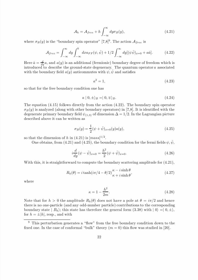
Ah = Afree + h

∞−∞

dyσB(y), (4.21)

where σB(y) is the “boundary spin operator” [7,8]9. The action Afree is

Afree = ∞−∞

dy

0

−∞dxaFF (ψ, ψ) + 1/2

∞−∞

dy[(ψψ)x=0 + aa]. (4.22)

Here a = ddya, and a(y) is an additional (fermionic) boundary degree of freedom which is

introduced to describe the ground-state degeneracy. The quantum operator a associatedwith the boundary field a(y) anticommutes with ψ, ψ and satisfies

a2 = 1, (4.23)

so that for the free boundary condition one has

a | 0, ±B =| 0, ∓B. (4.24)

The equation (4.15) follows directly from the action (4.22). The boundary spin operatorσB(y) is analyzed (along with other boundary operators) in [7,8]. It is identified with thedegenerate primary boundary field ψ(1,3) of dimension ∆ = 1/2. In the Lagrangian picturedescribed above it can be written as

σB(y) =1

2(ψ + ψ)x=0(y)a(y), (4.25)

so that the dimension of h in (4.21) is [mass]1/2.One obtains, from (4.21) and (4.25), the boundary condition for the fermi fields ψ, ψ,

id

dy(ψ − ψ)x=0 =

h2

2(ψ + ψ)x=0. (4.26)

With this, it is straightforward to compute the boundary scattering amplitude for (4.21),

Rh(θ) = i tanh(iπ/4 − θ/2)κ − i sinh θ

κ + i sinh θ, (4.27)

where

κ = 1

−

h2

2m

. (4.28)

Note that for h > 0 the amplitude Rh(θ) does not have a pole at θ = iπ/2 and hencethere is no one-particle (and any odd-number particle) contributions to the correspondingboundary state | Bh; this state has therefore the general form (3.38) with | 0 =| 0, ±,for h = ±|h|, resp., and with

9 This perturbation generates a “flow” from the free boundary condition down to thefixed one. In the case of conformal “bulk” theory (m = 0) this flow was studied in [20].

22

8/14/2019 9306002


K h(θ) = i tanh(θ/2)κ + cosh θ

κ − cosh θ. (4.29)

Again, this is not very surprising. The nonzero boundary magnetic field removes theground-state degeneracy; for h sufficiently small, the two-fold degenerate ground state

| 0, ±B of the “free” boundary splits into two non-degenerate states | 0B and | 1B,where | 1B can be interpreted as the boundary bound state. For 0 < h2 < 2m we canparametrize (4.28) as

κ = cos v. (4.30)

with real v, 0 < v < π/2. In this domain the amplitude (4.27) exhibits a pole in the physicalstrip at θ = i(π/2 − v) which is associated with the state | 1B. Physical interpretationof this boundary bound state is simple. For h = 0 the equilibrium “ground state” whichminimizes the free energy features an asymptotic behaviour σ(x, y)0 → +sign(h)σ asx

→ −∞. However, for h sufficiently small, there exists another stable equilibrum state

with σ(x, y)1 → −sign(h)σ as x → −∞. Although its free energy is higher by a positiveboundary term, it is indeed stable as in the infinite system there is no finite kinetics of decay(in a system finite in the y direction the decay probability is suppressed as exp(−mL cos v)).Clearly, the energies e0 and e1 of the states | 0B and | 1B have the meaning of specific(per unit boundary length) boundary free energies of these two equilibrum states. From(4.27) we have

e1 − e0 = m sin v. (4.31)

It is also clear that the expectation values ...1 can be obtained by analytic continuationof

...

0 from h to

−h. So, in this very domain

|h

|<

√2m “boundary histeresis”[21] can

be observed. It is possible to show that these expectation values can be computed as thematrix elements

...1 =B1 | ... | 1BB1 | 1B =

0′ | ... | B′h

0′ | B′h

, (4.32)

where the last expression contains the “excited boundary state”

| B′h = exp(

1

2

C

dθK h(θ)A†(−θ)A†(θ)) | 0′ (4.33)

with the integration taken along contour

Cshown in Fig.2, and

|0′

=

|0,

∓for h =

±|h

|.

As h approaches the “critical” value hc = √2m (i.e. v approaches π/2), the “boundarybound state” becomes weakly bound; e1 − e0 − m = −2m sin2(π/4 − v/2) → 0, and itseffective size ξ = (e1 − e0 − m)−1 diverges as (hc − h)−2. Correspondingly, the equilibriumstate ...1 developes large boundary fluctuations which propagate deep into the bulk,

σ(x, y)1 + σ ≃ exp(x/ξ) as x → −∞. (4.34)

At h = hc the boundary condition (4.26) reduces to

23

8/14/2019 9306002


∂

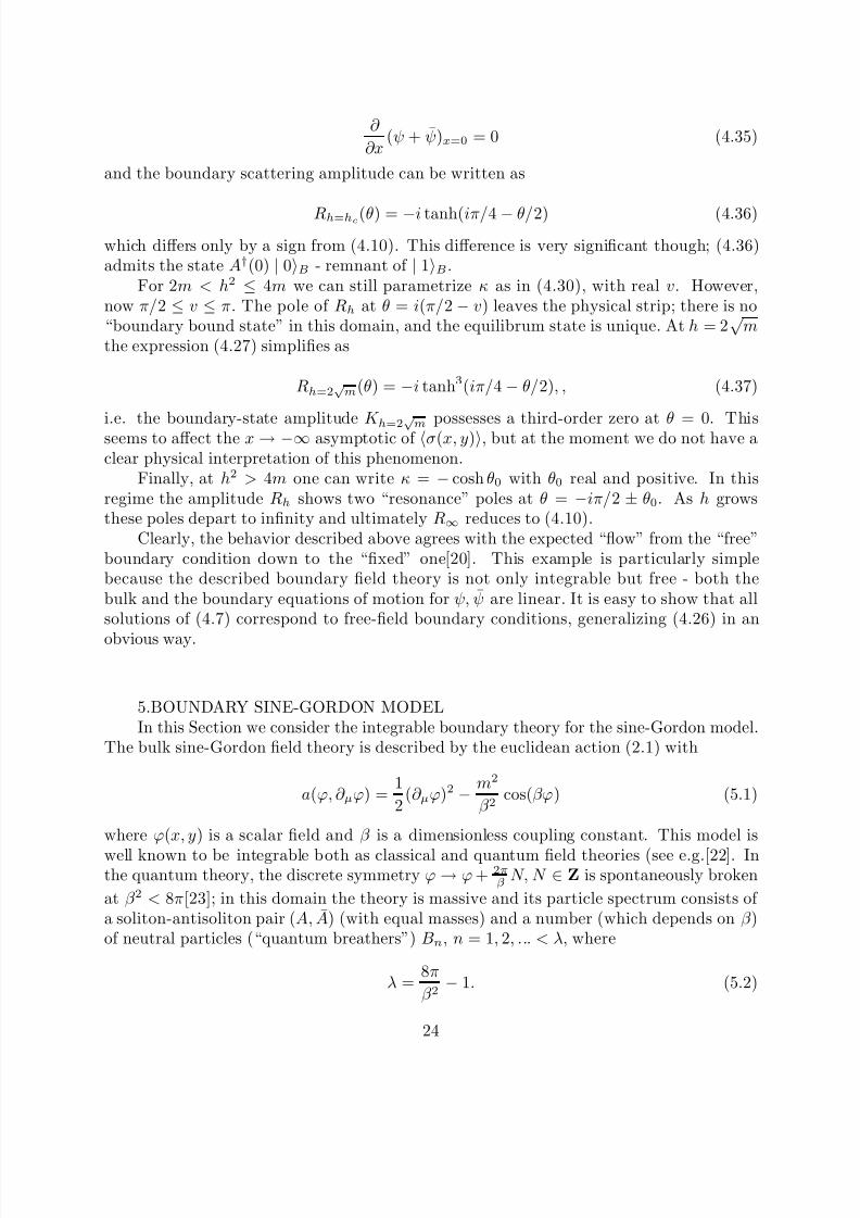
∂x(ψ + ψ)x=0 = 0 (4.35)

and the boundary scattering amplitude can be written as

Rh=hc(θ) = −i tanh(iπ/4 − θ/2) (4.36)

which differs only by a sign from (4.10). This difference is very significant though; (4.36)admits the state A†(0) | 0B - remnant of | 1B.

For 2m < h2 ≤ 4m we can still parametrize κ as in (4.30), with real v. However,now π/2 ≤ v ≤ π. The pole of Rh at θ = i(π/2 − v) leaves the physical strip; there is no“boundary bound state” in this domain, and the equilibrum state is unique. At h = 2

√m

the expression (4.27) simplifies as

Rh=2√m(θ) = −i tanh3(iπ/4 − θ/2), , (4.37)

i.e. the boundary-state amplitude K h=2√m possesses a third-order zero at θ = 0. Thisseems to affect the x → −∞ asymptotic of σ(x, y), but at the moment we do not have aclear physical interpretation of this phenomenon.

Finally, at h2 > 4m one can write κ = − cosh θ0 with θ0 real and positive. In thisregime the amplitude Rh shows two “resonance” poles at θ = −iπ/2 ± θ0. As h growsthese poles depart to infinity and ultimately R∞ reduces to (4.10).

Clearly, the behavior described above agrees with the expected “flow” from the “free”boundary condition down to the “fixed” one[20]. This example is particularly simplebecause the described boundary field theory is not only integrable but free - both thebulk and the boundary equations of motion for ψ, ψ are linear. It is easy to show that allsolutions of (4.7) correspond to free-field boundary conditions, generalizing (4.26) in an

obvious way.

5.BOUNDARY SINE-GORDON MODELIn this Section we consider the integrable boundary theory for the sine-Gordon model.

The bulk sine-Gordon field theory is described by the euclidean action (2.1) with

a(ϕ, ∂ µϕ) =1

2(∂ µϕ)2 − m2

β 2cos(βϕ) (5.1)

where ϕ(x, y) is a scalar field and β is a dimensionless coupling constant. This model is

well known to be integrable both as classical and quantum field theories (see e.g.[22]. Inthe quantum theory, the discrete symmetry ϕ → ϕ + 2π

β N, N ∈ Z is spontaneously broken

at β 2 < 8π[23]; in this domain the theory is massive and its particle spectrum consists of a soliton-antisoliton pair (A, A) (with equal masses) and a number (which depends on β )of neutral particles (“quantum breathers”) Bn, n = 1, 2, ... < λ, where

λ =8π

β 2− 1. (5.2)

24

8/14/2019 9306002


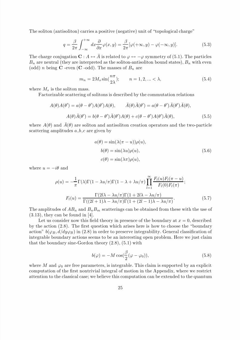
The soliton (antisoliton) carries a positive (negative) unit of “topological charge”

q =β

2π

+∞−∞

dx∂

∂xϕ(x, y) =

β

2π[ϕ(+∞, y) − ϕ(−∞, y)]. (5.3)

The charge conjugation C : A↔

A is related to ϕ↔ −

ϕ symmetry of (5.1). The particlesBn are neutral (they are interpreted as the soliton-antisoliton bound states), Bn with even(odd) n being C -even (C -odd). The masses of Bn are

mn = 2M s sin(nπ

2λ); n = 1, 2, ... < λ, (5.4)

where M s is the soliton mass.Factorizable scattering of solitons is described by the commutation relations

A(θ)A(θ′) = a(θ − θ′)A(θ′)A(θ), A(θ)A(θ′) = a(θ − θ′)A(θ′)A(θ),

A(θ)A(θ′) = b(θ−

θ′)A(θ′)A(θ) + c(θ−

θ′)A(θ′)A(θ), (5.5)

where A(θ) and A(θ) are soliton and antisoliton creation operators and the two-particlescattering amplitudes a,b,c are given by

a(θ) = sin(λ(π − u))ρ(u),

b(θ) = sin(λu)ρ(u), (5.6)

c(θ) = sin(λπ)ρ(u),

where u = −iθ and

ρ(u) = − 1π

Γ(λ)Γ(1 − λu/π)Γ(1 − λ + λu/π) ∞l=1

F l(u)F l(π − u)F l(0)F l(π)

;

F l(u) =Γ(2lλ − λu/π)Γ(1 + 2lλ − λu/π)

Γ((2l + 1)λ − λu/π)Γ(1 + (2l − 1)λ − λu/π). (5.7)

The amplitudes of ABn and BnBm scatterings can be obtained from these with the use of (3.13), they can be found in [4].

Let us consider now this field theory in presence of the boundary at x = 0, describedby the action (2.8). The first question which arises here is how to choose the “boundaryaction” b(ϕB, d/dyϕB) in (2.8) in order to preserve integrability. General classification of

integrable boundary actions seems to be an interesting open problem. Here we just claimthat the boundary sine-Gordon theory (2.8), (5.1) with

b(ϕ) = −M cos(β

2(ϕ − ϕ0)), (5.8)

where M and ϕ0 are free parameters, is integrable. This claim is supported by an explicitcomputation of the first nontrivial integral of motion in the Appendix, where we restrictattention to the classical case; we believe this computation can be extended to the quantum

25

8/14/2019 9306002


theory along the lines explained in Sect.2. We want to describe the factorizable boundaryscattering theory associated with (5.8).

The soliton (antisoliton) boundary scattering amplitudes can be encoded in the com-mutation relations (see Section 2)

A(θ)B = P +(θ)A(θ)B + Q+(θ)A(θ)B;

A(θ)B = P −(θ)A(θ)B + Q−(θ)A(θ)B. (5.9)

Here P +, Q+ (P −, Q−) are the amplitudes of soliton (antisoliton) one-particle boundaryscattering processes shown in Fig.23. Some comments are in order. Exept for the caseM = ∞ (see below), the boundary value ϕ(x = 0, y) is not fixed in the boundary fieldtheory (5.8)and hence the topological charge

q =β

2π

0−∞

dx∂

∂xϕ(x, y) (5.10)

is not conserved. Therefore the boundary scatterings are allowed to violate this chargeconservation by an even number. In particular, an incoming soliton can go away as anantisoliton and vice versa. The amplitudes Q± are introduced to describe these processes.The excceptional case is M = ∞ (“fixed” boundary condition); in this case we must haveQ± = 0. Also, at ϕ0 = 0(mod2π/β ) (and M = 0) the boundary interaction violatescharge-conjugation symmetry; that is why in the general case the amplitudes P +, Q+ andP −, Q− are expected to be different.

With (5.9), the boundary Yang-Baxter equation (3.25) leads to six distinct functionalequations,

Q+(θ′)c(θ + θ′)Q−(θ)a(θ − θ′) = Q−(θ′)c(θ + θ′)Q+(θ)a(θ − θ′), (5.11a)

P −(θ′)b(θ + θ′)P +(θ)c(θ − θ′) + P +(θ′)c(θ + θ′)P +(θ)b(θ − θ′) =

P −(θ′)c(θ + θ′)P −(θ)b(θ − θ′) + P +(θ′)b(θ + θ′)P −(θ)c(θ − θ′), (5.11b)

P +(θ′)a(θ+θ′)Q+(θ)c(θ−θ′)+Q+(θ′)b(θ+θ′)P +(θ)b(θ−θ′)+Q+(θ′)c(θ+θ′)P −(θ)c(θ−θ′) =

Q+(θ′)a(θ + θ′)P +(θ)a(θ − θ′) + P −(θ′)c(θ + θ′)Q+(θ)a(θ − θ′) (5.11c)

P +(θ′)a(θ+θ′)Q+(θ)b(θ−θ′)+Q+(θ′)b(θ+θ′)P +(θ)c(θ−θ′)+Q+(θ′)c(θ+θ′)P −(θ)b(θ−θ′) =

P +(θ′)b(θ + θ′)Q+(θ)a(θ − θ′), (5.11d)

(the other two are obtained from (5.11c), (5.11d) by + ↔ − substitution). The solutionto these equations is found in a recent paper[24]2; it reads

P +(θ) = cos(ξ + λu)R(u);

P −(θ) = cos(ξ − λu)R(u);

2 We learned about [24] after we had found this solution independently.

26

8/14/2019 9306002


Q+(θ) =k+2

sin(2λu)R(u);

Q−(θ) =k−2

sin(2λu)R(u), (5.12)

where again u =−

iθ; ξ, k±

are free parameters and R(u) is an arbitrary function3.The free parameters in (5.12) have to be related to the parameters of the boundary

action. The solution (5.12) seems to contain one parameter more than the action (5.8). Itis easy to see however that one of the two parameters k± in (5.12) can be removed by anappropriate gauge transformation

A(θ) → eiαA(θ), A(θ) → e−iαA(θ) (5.13)

which leaves all the charge-conserving amplitudes unchanged and transforms the ampli-tudes Q± as

Q+(θ)→

e−2iαQ+(θ); Q−

(θ)→

e+2iαQ−

(θ). (5.14)

Considered from the Lagrangian point of view, this transformation amounts to adding atotal derivative term to the boundary action density (5.8),

b(ϕ) → b(ϕ) +2πα

β

d

dyϕ. (5.15)

We use this freedom to set k+ = k− = k. This leaves us with two parameters, ξ and k,which correspond to the two-parameters M and ϕ0 in (5.8).

The function R(u) in (5.12) can be determined with the use of the“boundary unitarity”and the “boundary cross-unitarity” equations (3.26) and (3.35). These equations reduceto

R(u)R(−u) = [cos2(ξ) − sin2(λu) − k2 sin2(λu)cos2(λu)]−1; (5.16)

K (u) = sin λ(π + 2u)ρ(2u)K (−u); K (u) = R(π/2 − u). (5.17)

It is not difficult to solve these equations. In fact, it is convenient to solve (5.16) and (5.17)“separately”. Let us factorize the function R(u) as

R(u) = R0(u)R1(u); K (u) = K 0(u)K 1(u), (5.18)

where K 0(u) = R0(π/2 − u), K 1(u) = R1(π/2 − u) so that these factors satisfy

R0(u)R0(−u) = 1; K 0(u) = sin λ(π + 2u)ρ(2u)K 0(−u) (5.19)

and

R1(u)R1(−u) = [cos2(ξ) − (1 + k2)sin2(λu) + k2 sin4(λu)]−1; K 1(u) = K 1(−u). (5.20)

3 This is the general solution for generic λ. For integer λ there are additional solutions.

27

8/14/2019 9306002


The equations (5.19) do not contain the boundary parameters ξ and k; the solution canbe written as

R0(u) = F 0(u)/F 0(−u);

F 0(u) =Γ(1

−2λu/π)

Γ(λ − 2λu/π)×∞k=1

Γ(4λk − 2λu/π)Γ(1 + 4λk − 2λu/π)Γ(λ(4k + 1))Γ(1 + λ(4k − 1))

Γ(λ(4k + 1) − 2λu/π)Γ(1 + λ(4k − 1) − 2λu/π)Γ(1 + 4λk)Γ(4λk)(5.21)

The factor R0 contains the poles in the “physical strip” 0 < u < π/2 located at u = un =nπ/2λ; n = 1, 2,... < λ. Appearence of these poles is very well expected. In the genericcase, the boundary state | B associated with the boundary condition (5.8) is expectedto contain the contributions of the zero-momentum particles Bn, which leads to the poles(3.41). So, these poles of R0 correspond to the diagrams in Fig.24. Note that these polesshould not appear in the amplitudes Q

±and the factor sin(2λu) in (5.12) takes care of

this.The equation (5.20) contains all the information about the boundary condition (i.e.

the parameters ξ and k). Its solution can be written as

R1(u) =1

cos ξσ(η, u)σ(iϑ,u) (5.22)

where

σ(x, u) =Π(x,π/2 − u)Π(−x,π/2 − u)Π(x, −π/2 + u)Π(−x, −π/2 + u)

Π2

(x,π/2)Π2

(−x,π/2)

;

Π(x, u) =∞l=0

Γ(1/2 + (2l + 1/2)λ + x/π − λu/π)Γ(1/2 + (2l + 3/2)λ + x/π)

Γ(1/2 + (2l + 3/2)λ + x/π − λu/π)Γ(1/2 + (2l + 1/2)λ + x/π)(5.23)

solves

σ(x, u)σ(x, −u) = [cos(x + λu)cos(x − λu)]−1; σ(x,π/2 − u) = σ(x,π/2 + u), (5.24)

and the parameters η and ϑ are determined through the equations

cos(η) cosh(ϑ) = − 1

kcos ξ; cos2(η) + cosh2(ϑ) = 1 +

1

k2. (5.25)

The above boundary S-matrix has a very rich structure. The factor σ(iϑ,u) in (5.22)brings in an infinite set of singularities at complex values of u; some of these complexpoles probably can be interpreted as resonance states of the boundary. The factor σ(η, u)exhibits infinitely many poles at real u; depending on the parameter η, some of these polescan occur in the “physical strip” 0 < u < π/2 thus giving rise to the boundary bound

28

8/14/2019 9306002


states. We did not carry out a complete analysis of the possible boundary phenomenadescribed by this S-matrix. In order to do this one must find the an exact relation betweenthe parameters M and ϕ0 in the boundary action and ξ and k (or η and ϑ) in the S-matrix.A brief analysis shows that in the general case this relation is very complicated. We leavethis problem for future studies. Here we analyze only two particular cases.

a). “Fixed” boundary condition ϕ(x, y)x=0 = ϕ0 can be obtained from (5.8) in thelimit M = ∞. In this case the topological charge is conserved and the amplitudes Q± in(5.9) must vanish. Hence this case corresponds to k = 0. We have two amplitudes, P + andP − which describe soliton scattering processes schematically shown in Fig.25. For k = 0,the “resonance” factor σ(iϑ,u) disappears and the equation (5.22) simplifies as

R1(u) =1

cos ξσ(ξ, u), (5.26)

where ξ is related in some way to ϕ0. Obviously, ϕ0 = 0 corresponds to ξ = 0 as at ϕ0 = 0the boundary theory respects C symmetry and we must have P + = P −. At ξ = 0 the

function R1(u) does not exhibit any poles in the physical strip (and hence there are noboundary bound states), the nearest singularity being the double pole at u = −π/2λ. Atξ = 0 (i.e. ϕ0 = 0) this double pole splits into two simple poles at u = u± = −π/2λ ± ξ/λ.Note that due to the factors cos(ξ ± λu) in (5.12) the pole θ = iu+ (θ = iu−) appears onlyin P + (P −). At ξ > π/2 the pole at θ = iu+ enters the physical strip. Appearence of such a“boundary bound state” is well expected. For 0 < ϕ0 < π/β the ground state | 0B of theboundary sine-Gordon theory is characterized by the asymptotic behaviour ϕ(x, y)B → 0as x → −∞. Classically, there is another stable state with ϕ(x, y) → 2π/β as x → −∞.If ϕ0 is small (compared to the quantum parameter β ), quantum fluctuations can destroyits stability. However, if ϕ0 is not too small, this state is expected to be stable in thequantum theory, too. At ϕ0 = π/β this state has the same energy as the ground state

which hence becomes degenerate. In this case the amplitude P +(θ) has to have a pole atθ = iπ/2 corresponding to the “emission” of a zero-momentum soliton by the associatedboundary state, as is explained in Sect.3. We can conclude that ϕ0 = π/β corresponds tothe case u+ = π/2. Assuming a linear relation between ξ and ϕ0, we find

ξ =4π

β ϕ0. (5.27)

Let us stress that the assumed linear relation (and hence (5.27)) is no more than a conjecture. Also, the relation (5.27) is conjectured only for the “fixed” case M = ∞; it is notexpected to hold in the general case of finite M .

b). “Free” boundary condition corresponds to M = 0 in (5.8). In this case the fullaction enjoys the symmetry ϕ → −ϕ (C symmetry) and hence we must have P + = P − =P free and Q+ = Q− = Qfree, i.e. we have to choose ξ = 0. Note that under this choice thefactors cos(λθ) in (5.12) cancel the poles at θ = iu2n+1 of the factor (5.21). This agreeswith the expectation that in the C -symmetric case the boundary state can not emit theC -odd particles B2n+1

3. In addition, in the “free” case one expects all the amplitudes

3 In fact, it is easy to argue that in general the choice ξ = 0 corresponds to the C

29

8/14/2019 9306002


(5.12) to have a pole at θ = iπ/2, for exactly the same reason which we discussed in theprevious Section. To ensure this property one has to choose η = π

2 (λ + 1) (and ϑ = 0), i.e.k = [sin(πλ/2)]−1. So in the “free” case the amplitudes (5.12) can be written as

P free(θ) = sin(πλ/2)Rfree(u); Qfree(θ) = sin(λu)Rfree(u) (5.28)

where

Rfree(u) =cos(λu)

sin(λπ/2)R0(u)σ(4π2/β 2, u)σ(0, u). (5.29)

6.DISCUSSIONObviously, there is much room for further development.More detailed analysis of “integrable boundary conditions” is needed. In Section

2 we assumed that the boundary action b in (2.8) depends only on boundary valuesϕB(y), d/dyϕB(y) of the “bulk” field ϕ(x, y). In general, the boundary action can containalso specific boundary degrees of freedom. Clearly, this provides more possibilities for theintegrable boundary field theories.

Further study of possible solutions to Boundary Yang-Baxter equations ((3.25) is of much interest. A new class of solutions is found in a recent paper [24].

Many integrable “bulk” theories exhibit nonlocal integrals of motion of fractional spin[25-27], along with the local ones. Analysis of these nonlocal integrals provides valuableinformation about the S-matrix. We expect that the nonlocal integrals of motion exist insome integrable boundary field theories. A natural place to look for the nonlocal IM isboundary sine-Gordon model considered in Section 5. As in the case of bulk sine-Gordon

theory, where nonlocal IM generate the so-called “affine quantum group symmetry”[27],appropriate modifications of these IM could help to find an exact relation between theparameters of the action (M and ϕ0 in (5.8)) and of the S-matrix (ξ, k in (5.12))(whichwe found very difficult to guess).

The most interesting problem is how to extract any off-shell data from the S-matrix.In the bulk theory, two approaches have proven to be the most successfull. One is the“formfactor bootstrap” proposed by Smirnov[27]. It would be interesting to generalize theformfactor bootstrap equations to the case of integrable boundary field theory, both forbulk operators in presence of boundary and for boundary operators. Another approach isknown as “thermodinamic Bethe anzats”(TBA)[29]. At the present stage of development,it is capable of providing the ground state energy of a finite-size system (with spatial

coordinate compactified on a circle), once the S-matrix is known. This approach canbe generalized in different ways to incorporate the boundary effects. In particular, theexpression (3.38) for the boundary state allows one to find the analog of TBA equationsfor spatially finite systems with integrable boundaries. We intend to study these equationselsewhere.

-symmetric boundary action (5.8) with ϕ0 = 0. Even in this case the relation between M and k seems to be rather complicated.

30

8/14/2019 9306002


It was understood recently that many interesting “massless flows” in the bulk the-ory can be described in terms of “massless factorizable S-matrices”, through TBA equa-tions[30]. This approach can be modified to incorporate “massless boundary S-matrices”[31], thus providing the possibility of a similar description of the “boundary flows”[32].

After this work was finished we received a recent paper [31] where some results of

Section 3 (notably, the “boundary bootstrap equation”(3.40)) are obtained. However, the“boundary cross-unitarity equation” (3.35) (which we think to be the most significant of our results) is not considered there; that is why we decided that our paper is still worthpublishing.

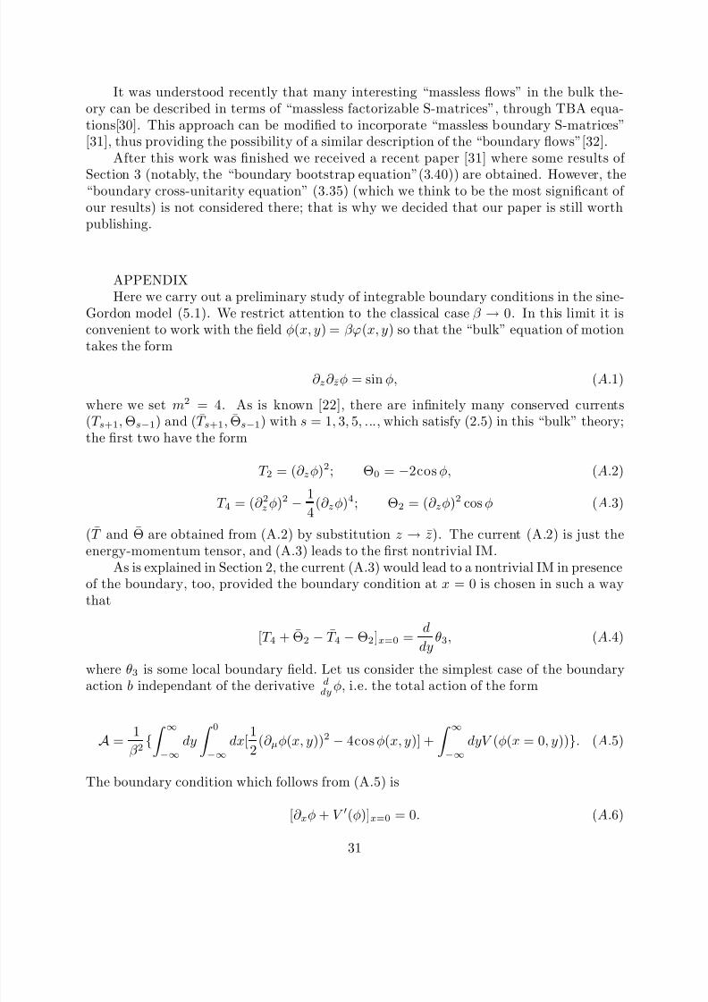
APPENDIXHere we carry out a preliminary study of integrable boundary conditions in the sine-

Gordon model (5.1). We restrict attention to the classical case β → 0. In this limit it isconvenient to work with the field φ(x, y) = βϕ(x, y) so that the “bulk” equation of motion

takes the form

∂ z∂ zφ = sin φ, (A.1)

where we set m2 = 4. As is known [22], there are infinitely many conserved currents(T s+1, Θs−1) and (T s+1, Θs−1) with s = 1, 3, 5, ..., which satisfy (2.5) in this “bulk” theory;the first two have the form

T 2 = (∂ zφ)2; Θ0 = −2cos φ, (A.2)

T 4 = (∂ 2zφ)2 − 1

4(∂ zφ)4; Θ2 = (∂ zφ)2 cos φ (A.3)

(T and Θ are obtained from (A.2) by substitution z → z). The current (A.2) is just theenergy-momentum tensor, and (A.3) leads to the first nontrivial IM.

As is explained in Section 2, the current (A.3) would lead to a nontrivial IM in presenceof the boundary, too, provided the boundary condition at x = 0 is chosen in such a waythat

[T 4 + Θ2 − T 4 − Θ2]x=0 =d

dyθ3, (A.4)

where θ3 is some local boundary field. Let us consider the simplest case of the boundaryaction b independant of the derivative d

dyφ, i.e. the total action of the form

A =1

β 2{ ∞−∞

dy

0−∞

dx[1

2(∂ µφ(x, y))2 − 4cos φ(x, y)] +

∞−∞

dyV (φ(x = 0, y))}. (A.5)

The boundary condition which follows from (A.5) is

[∂ xφ + V ′(φ)]x=0 = 0. (A.6)

31

8/14/2019 9306002


With this, the l.h.s of (A.4) can be written (up to an overall numerical factor) as

V ′(φ)(∂ yφ)3 + 8V ′′(φ)(∂ 2yyφ)(∂ yφ) − [(V ′(φ))3 + 4V ′′(φ)sin φ + 2V ′(φ)cos φ](∂ yφ). (A.7)

This reduces to a total d/dy derivative if the function V (φ) satisfies

4V ′′(φ) + V (φ) = 0, (A.8)

that is

V (φ) = −Λcos(φ − φ0

2), (A.9)

where Λ and φ0 are constants. Returning to the original normalization, one gets (5.8).

32

8/14/2019 9306002


REFERENCES.1.K.Binder, in “Phase Transitions and Critical Phenomena”, v.8, C.Domband J.Lebowitz ed., Academic Press, London, 1983.2.C.G.Callan, L.Thorlacius. Nucl.Phys.B329(1990),117.3.E.Witten. Phys.Rev.46D(1992)p.5467., K.Li, E.Witten. Preprint

IASSNS-HEP-93/7, 1993.4.A.B.Zamolodchikov, Al.B.Zamolodchikov. Ann.Phys.120 (1979), 253.5.A.B.Zamolodchikov. Advanced Studies in Pure Mathematics 19 (1989), 641.6.J.Cardy. “Conformal Invariance and Surface Critical Behavior”, in“Conformal Invariance and Applications to Statistical Mechanics”,E.Itzykson, H.Saleur, J.B.Zuber eds., World Scientific, 1988.7.J.Cardy. Nucl.Phys.B324(1989)p. 581.8.J.Cardy, D.Lewellen. Phys.Lett. 259B (1991) p.274.9.E.Ogievetsky, N.Reshetikhin, P.Wiegmann. Nucl.Phys B280 [FS 18] (1987), p.45.10.V.Fateev, A.Zamolodchikov. “Conformal Field Theory and Purely

Elastic S-Matrices”, in “Physics and Mathematics of Strings”,memorial volume for Vadim Knizhnik, L.Brink, D.Friedan, A.Polyakoveds., World Scientific, 1989.11.J.Cardy, G.Mussardo. Phys. Lett. B225 (1989) 243.12.P.Freund, T.Classen, E.Melzer. Phys.Lett. 229B (1989) p.243;G.Sotkov, C.Zhu. Phys.Lett. 229B (1989) p.391; P.Christe, G.Mussardo.Nucl.Phys. B330 (1990) p.465.13.I.Cherednik. Theor.Math.Phys., 61, 35 (1984) p.977.14.L.Takhtadjian, L.Faddeev. Usp.Mat.Nauk. 34 (1979) p.13.15.E.Sklyanin. J.Phys. A:Math.Gen. 21 (1988) p.237516.L.Mezincescu, R.Nepomechie. Int.J.Mod.Phys. A6, 5231 (1991).

17.P.Kulish, E.Sklyanin. “Algebraic Structures related to ReflectionEquation”. Preprint YITP/K-980, 1992.18.J.Cardy. Phys.Rev.Lett. 54 (1985) p.1354.19.M.Sato, T.Miwa, M.Jimbo. Proc. Japan Acad., 53A (1977), 6.20.I.Affleck, A.Ludwig. “Universal Non-integer Groundstate Degeneracyin Critical Quantum Systems”. Preprint UBCTP-91-007, 1991.21.B.McCoy, T.T.Wu. “The two-dimensional Ising Model”, HarwardUniversity Press. 1973.22.L.Takhtadjian, L.Faddeev. Theor.Math.Phys. 21, (1974) p.160.,V.Korepin, L.Faddeev. Theor.Math.Phys. 25 (1975) p.147.

23.S.Coleman. Phys.Rev. D11, (1975) p.2088.24.H.J.DeVega, A.Gonzalez Ruiz. Preprint LPTHE 92-45.25.M.Luscher. Nucl.Phys. B135 (1978) p.1.26.A.B.Zamolodchikov.”Fractional-Spin Integrals of Motion in PerturbedConformal Field Theory”, in “Fields, Strings and Quantum Gravity”,H.Guo, Z.Qiu, H.Tye eds., Gordon and Breach, 1989.27.D.Bernard, A.LeClaire. Commun.Math.Phys., 142 (1991) p.99.28.F.Smirnov. “Formfactors in Completely Integrable Models of QFT”,

33

8/14/2019 9306002


Adv. Series in Math.Phys.14, World Scientific, 1992.29.Al.Zamolodchikov. Nucl.Phys. B342 (1990) p.695.30.Al.Zamolodchikov. Nucl.Phys. B385 (1991) p.619., A.Zamolodchikov,Al.Zamolodchikov. Nucl.Phys. B379 (1992) p.602.31.P.Fendley. “Kinks in the Kondo Problem”. Preprint BUHEP-93-10.

32.A.Fring, R.Koberle. “Factorized Scattering in the Presence of Reflecting Boundaries”. Preprint USP-IFQSC/TH/93-06, 1993.

34

8/14/2019 9306002


1

2

FIG-1

12

1

2

y

y

y

C

C

C

(θ)

FIG-2

21

21

12

21a

a a

b b

θ

S

bb

a

’θ

θ

312

3

132

1

bbbb

aaaa

FIG-3

35

8/14/2019 9306002


12

1 2

21

21aa

bb

δ δ

−θ

θ

FIG-4

bb

aa

2

1

θ

π−θi

FIG-5

bb

a

12

21

FIG-6

1 2a aciu

c

bb

aa

FIG-7

21

1a a

cf

c

aa

36

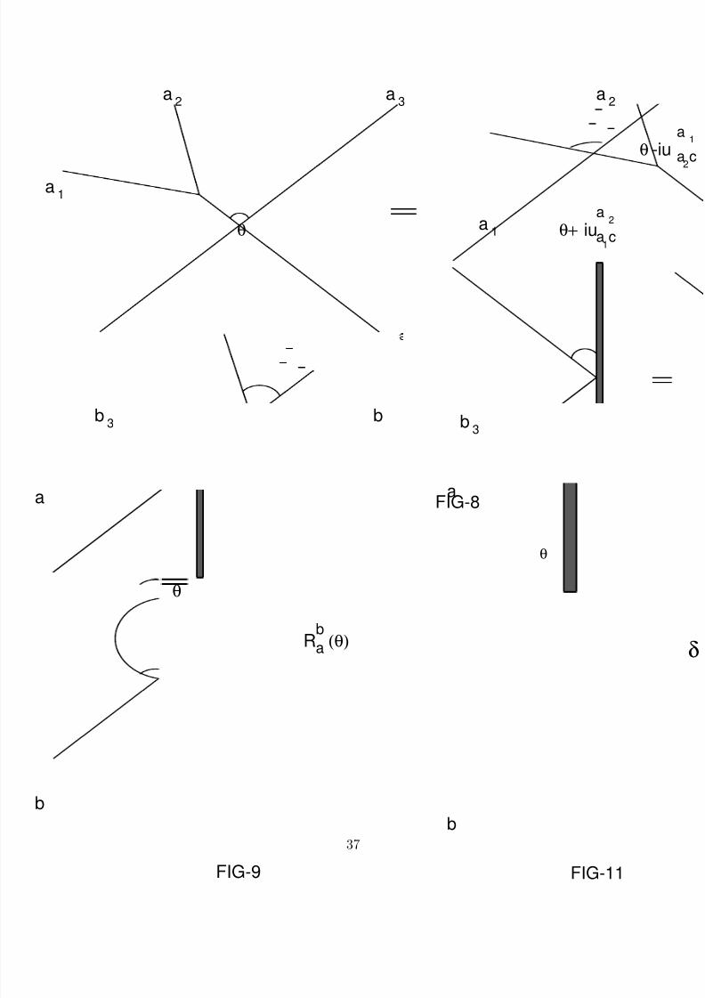
8/14/2019 9306002


θ

FIG-8

1

2

-

a

a ciuθ+θ

2

1

33

32

1

bbb

a

a

aa

a

b

a

(θ)

FIG-9

a

bR

θ

−θ

θ

FIG-11

b

a

37

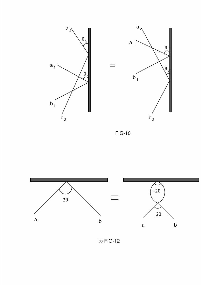
8/14/2019 9306002


2

1

1

2

2

1

1

2

2

1

1

2

FIG-10

b

b

a

a

b

b

a

a

θ

θ

θ

θ

2θ

−2θ

2θ

FIG-12

baba

38

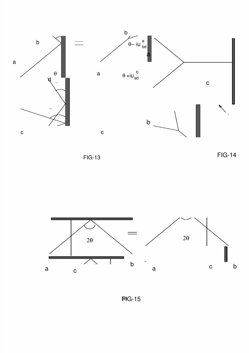
8/14/2019 9306002


b

ad

b

bd

aiu

+iu

FIG-13

a

cc

d

b

a

θ−

θθ

FIG-1

c

b

a

2θ2θ

FIG-15

cab

ca

39

8/14/2019 9306002


2θ

θ

10θ

1

21

FIG-16

ccc

FIG-17

α

α

b

a

a0iv

(θα

β

a

b

β

α

θ

R

FIG-18

b

a

40

8/14/2019 9306002


θ

b’

b

a

b’

b

a

FIG-19

β

θ

α

β

γ

α

FIG-20

αa

β

β

α

g

a

FIG

41

8/14/2019 9306002


iv

π

2

θ

θ

FIG-22

C

i

Im

42

8/14/2019 9306002


FIG-23

(θ)

θθ

θθ

(θ)

(θ)

(θ)

-

+

-

+

Q

Q

P

P

FIG-24

nB

A

A

43

8/14/2019 9306002


A

FIG-25

β

−2π

0

0

ϕ

0

0

ϕ

β

2π

AA

A

-P

+P

44

8/14/2019 9306002


This figure "fig1-1.png" is available in "png"format from:

http://arXiv.org/ps/hep-th/9306002v2

http://arxiv.org/ps/hep-th/9306002v2


8/14/2019 9306002






9306002

Documents