978-1-58503-591-5 -- catia v5 tutorials in - sdc publications
TRANSCRIPT

CATIA V5 Tutorials Mechanism Design & Animation
Release 19
Nader G. Zamani University of Windsor
Jonathan M. Weaver University of Detroit Mercy
SDC
Schroff Development Corporation www.schroff.com
Better Textbooks. Lower Prices.
PUBLICATIONS
CATIA V5 Tutorials in Mechanism Design and Animation 4-1
Chapter 4
Slider Crank Mechanism

4-2 CATIA V5 Tutorials in Mechanism Design and Animation
Introduction In this tutorial you create a slider crank mechanism using a combination of revolute and cylindrical joints. You will also experiment with additional plotting utilities in CATIA. 1 Problem Statement A slider crank mechanism, sometimes referred to as a three-bar-linkage, can be thought of as a four bar linkage where one of the links is made infinite in length. The piston based internal combustion is based off of this mechanism. The analytical solution to the kinematics of a slider crank can be found in elementary dynamics textbooks. In this tutorial, we aim to simulate the slider crank mechanism shown below for constant crank rotation and to generate plots of some of the results, including position, velocity, and acceleration of the slider. The mechanism is constructed by assembling four parts as described later in the tutorial. In CATIA, the number and type of mechanism joints will be determined by the nature of the assembly constraints applied. There are several valid combinations of joints which would produce a kinematically correct simulation of the slider crank mechanism. The most intuitive combination would be three revolute joints and a prismatic joint. From a degrees of freedom standpoint, using three revolute joints and a prismatic joint redundantly constrains the system, although the redundancy does not create a problem unless it is geometrically infeasible, in this tutorial we will choose an alternate combination of joints both to illustrate cylindrical joints and to illustrate that any set of joint which removes the appropriate degrees of freedom while providing the capability to drive the desired motions can be applied. In the approach suggested by this tutorial, the assembly constraints will be applied in such a way that two revolute joints and two cylindrical joints are created reducing the degrees of freedom are reduced to one. This remaining degree of freedom is then removed by declaring the crank joint (one of the cylindrical joints in our approach) as being angle driven. An exercise left to the reader is to create the same mechanism using three revolute joints and one prismatic joint or some other suitable combination of joints. We will use the Multiplot feature available in CATIA is used to create plots of the simulation results where the abscissa is not necessarily the time variable.
Revolute
Revolute
Cylindrical
Cylindrical

Slider Crank Mechanism 4-3
2 Overview of this Tutorial In this tutorial you will:
1. Model the four CATIA parts required. 2. Create an assembly (CATIA Product) containing the parts. 3. Constrain the assembly in such a way that only one degree of freedom is
unconstrained. This remaining degree of freedom can be thought of as rotation of the crank.
4. Enter the Digital Mockup workbench and convert the assembly constraints into two revolute and two cylindrical joints.
5. Simulate the relative motion of the arm base without consideration to time (in other words, without implementing the time based angular velocity given in the problem statement).
6. Add a formula to implement the time based kinematics associated with constant angular velocity of the crank.
7. Simulate the desired constant angular velocity motion and generate plots of the kinematic results.
4-4 CATIA V5 Tutorials in Mechanism Design and Animation
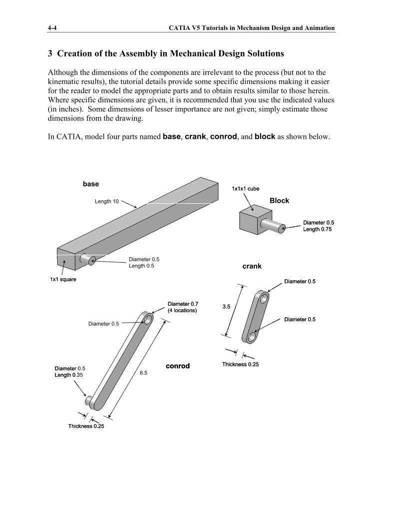
3 Creation of the Assembly in Mechanical Design Solutions Although the dimensions of the components are irrelevant to the process (but not to the kinematic results), the tutorial details provide some specific dimensions making it easier for the reader to model the appropriate parts and to obtain results similar to those herein. Where specific dimensions are given, it is recommended that you use the indicated values (in inches). Some dimensions of lesser importance are not given; simply estimate those dimensions from the drawing. In CATIA, model four parts named base, crank, conrod, and block as shown below.
1x1 square
Diameter 0.5Length 0.5
Length 10
1x1 square
Diameter 0.5Length 0.5
Length 10
base
1x1x1 cube
Diameter 0.5Length 0.75
1x1x1 cube
Diameter 0.5Length 0.75
Block
Diameter 0.5
Diameter 0.5
3.5
Thickness 0.25
Diameter 0.5
Diameter 0.5
3.5
Thickness 0.25
crank
Diameter 0.7(4 locations)
Diameter 0.5
Diameter 0.5Length 0.35 6.5
Thickness 0.25
conrod
Diameter 0.7(4 locations)
Diameter 0.5
Diameter 0.5Length 0.35 6.5
Thickness 0.25
conrod
Slider Crank Mechanism 4-5
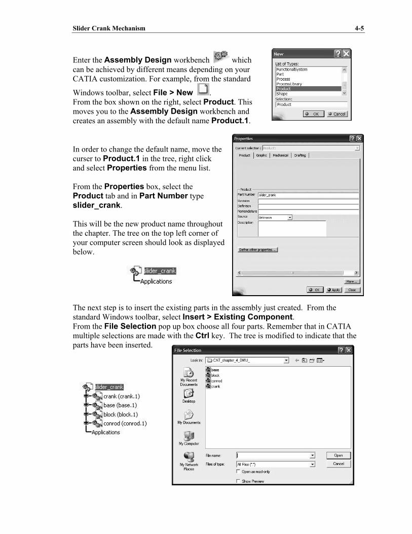
Enter the Assembly Design workbench which can be achieved by different means depending on your CATIA customization. For example, from the standard
Windows toolbar, select File > New . From the box shown on the right, select Product. This moves you to the Assembly Design workbench and creates an assembly with the default name Product.1. In order to change the default name, move the curser to Product.1 in the tree, right click and select Properties from the menu list. From the Properties box, select the Product tab and in Part Number type slider_crank. This will be the new product name throughout the chapter. The tree on the top left corner of your computer screen should look as displayed below. The next step is to insert the existing parts in the assembly just created. From the standard Windows toolbar, select Insert > Existing Component. From the File Selection pop up box choose all four parts. Remember that in CATIA multiple selections are made with the Ctrl key. The tree is modified to indicate that the parts have been inserted.

4-6 CATIA V5 Tutorials in Mechanism Design and Animation
Note that the part names and their instance names were purposely made the same. This practice makes the identification of the assembly constraints a lot easier down the road. Depending on how your parts were created earlier, on the computer screen you have the four parts all clustered around the origin. You may have to use the Manipulation icon
in the Move toolbar to rearrange them as desired. The best way of saving your work is to save the entire assembly. Double click on the top branch of the tree. This is to ensure that you are in the Assembly Design workbench.
Select the Save icon . The Save As pop up box allows you to rename if desired. The default name is the slider_crank.
Slider Crank Mechanism 4-7
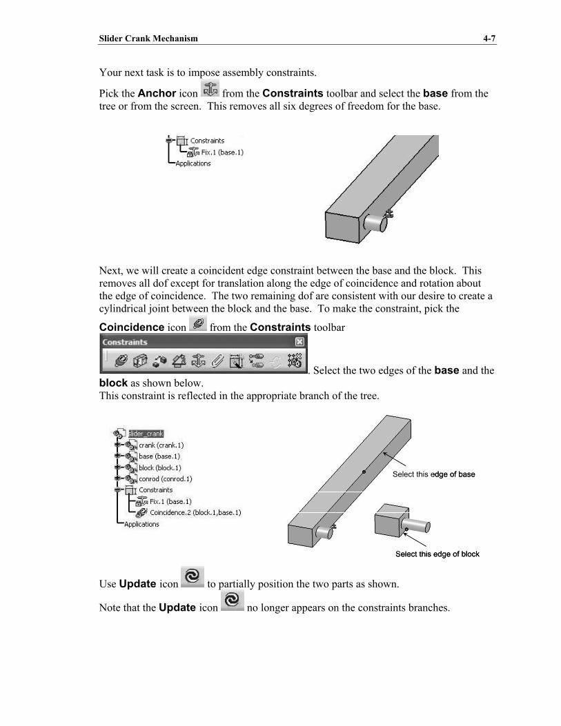
Your next task is to impose assembly constraints.
Pick the Anchor icon from the Constraints toolbar and select the base from the tree or from the screen. This removes all six degrees of freedom for the base. Next, we will create a coincident edge constraint between the base and the block. This removes all dof except for translation along the edge of coincidence and rotation about the edge of coincidence. The two remaining dof are consistent with our desire to create a cylindrical joint between the block and the base. To make the constraint, pick the
Coincidence icon from the Constraints toolbar
. Select the two edges of the base and the block as shown below. This constraint is reflected in the appropriate branch of the tree.
Use Update icon to partially position the two parts as shown.
Note that the Update icon no longer appears on the constraints branches.
Select this edge of block
Select this edge of base
Select this edge of block
Select this edge of base

4-8 CATIA V5 Tutorials in Mechanism Design and Animation
Depending on how your parts were constructed the block may end up in a position quite
different from what is shown below. You can always use the Manipulation icon to position it where desired followed by Update if necessary.
You will now impose assembly constraints between the conrod and the block. Recall that we ultimately wish to create a revolute joint between these two parts, so our assembly constraints need to remove all the dof except for rotation about the axis.
Pick the Coincidence icon from Constraints toolbar. Select the axes of the two cylindrical surfaces as shown below. Keep in mind that the easy way to locate the axis is to point the cursor to the curved surfaces.
The coincidence constraint just created removes all but two dof between the conrod and the base. The two remaining dof are rotation about the axis (a desired dof) and translation along the axis (a dof we wish to remove in order to produce the desired
revolute joint). To remove the translation, pick the Coincidence icon from the Constraints toolbar and select the surfaces shown on the next page. If your parts are
Select the axis of the cylinder on the block
Select the axis of the hole on the conrod

Slider Crank Mechanism 4-9
originally oriented similar to what is shown, you will need to choose Same for the Orientation in the Constraints Definition box so that the conrod will flip to the desired orientation upon an update. The tree is modified to reflect this constraint.
Use Update icon to partially position the two parts as shown below. Note that upon updating, the conrod may end up in a location which is not convenient for
the rest of the assembly. In this situation the Manipulation icon can be used to conveniently rearrange the conrod orientation.
Choose the end surface of the cylinder
Choose the back surface of the conrod (surface not visible in this view)
4-10 CATIA V5 Tutorials in Mechanism Design and Animation
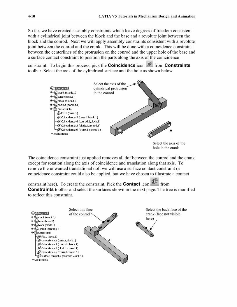
So far, we have created assembly constraints which leave degrees of freedom consistent with a cylindrical joint between the block and the base and a revolute joint between the block and the conrod. Next we will apply assembly constraints consistent with a revolute joint between the conrod and the crank. This will be done with a coincidence constraint between the centerlines of the protrusion on the conrod and the upper hole of the base and a surface contact constraint to position the parts along the axis of the coincidence
constraint. To begin this process, pick the Coincidence icon from Constraints toolbar. Select the axis of the cylindrical surface and the hole as shown below.
The coincidence constraint just applied removes all dof between the conrod and the crank except for rotation along the axis of coincidence and translation along that axis. To remove the unwanted translational dof, we will use a surface contact constraint (a coincidence constraint could also be applied, but we have chosen to illustrate a contact
constraint here). To create the constraint, Pick the Contact icon from Constraints toolbar and select the surfaces shown in the next page. The tree is modified to reflect this constraint.
Select the axis of the cylindrical protrusion in the conrod
Select the axis of the hole in the crank
Select this face of the conrod
Select the back face of the crank (face not visible here)
Slider Crank Mechanism 4-11
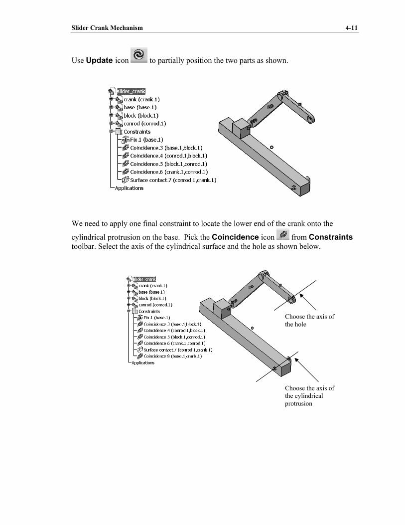
Use Update icon to partially position the two parts as shown.
We need to apply one final constraint to locate the lower end of the crank onto the
cylindrical protrusion on the base. Pick the Coincidence icon from Constraints toolbar. Select the axis of the cylindrical surface and the hole as shown below.
Choose the axis of the hole
Choose the axis of the cylindrical protrusion
4-12 CATIA V5 Tutorials in Mechanism Design and Animation
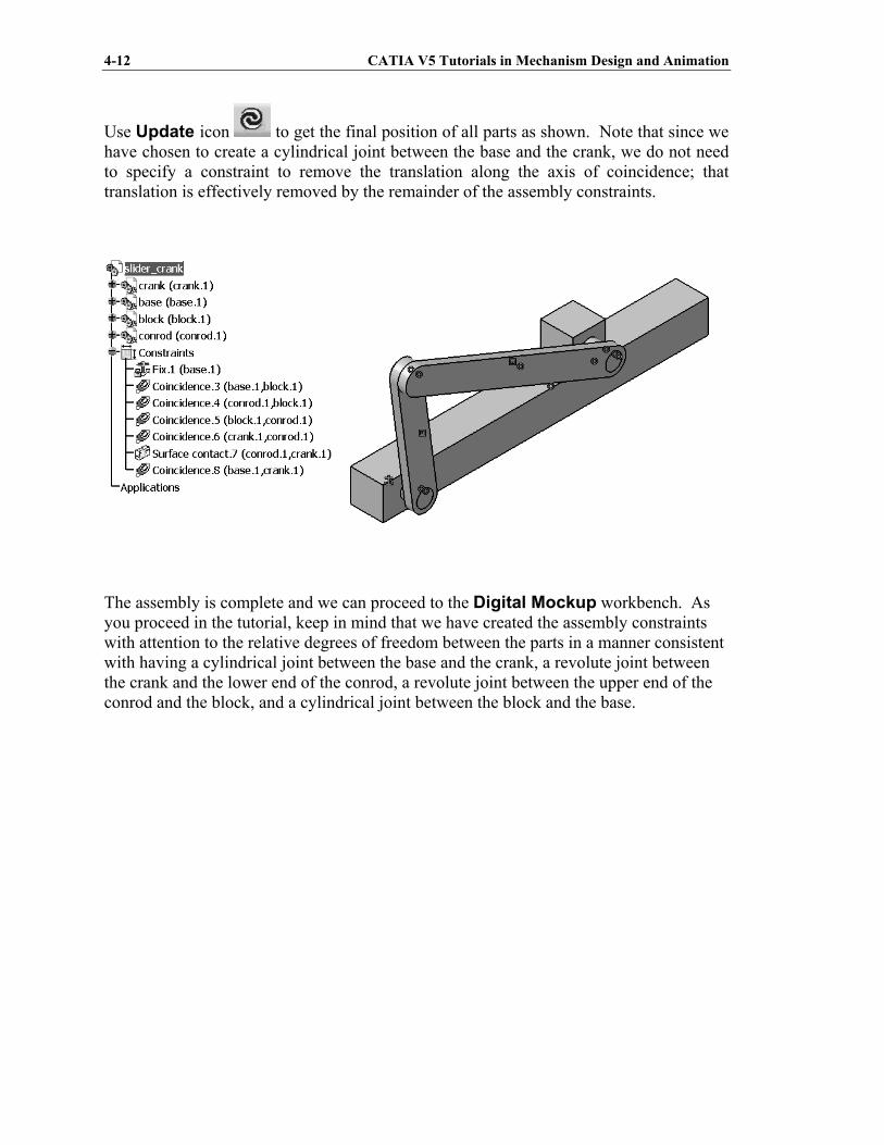
Use Update icon to get the final position of all parts as shown. Note that since we have chosen to create a cylindrical joint between the base and the crank, we do not need to specify a constraint to remove the translation along the axis of coincidence; that translation is effectively removed by the remainder of the assembly constraints.
The assembly is complete and we can proceed to the Digital Mockup workbench. As you proceed in the tutorial, keep in mind that we have created the assembly constraints with attention to the relative degrees of freedom between the parts in a manner consistent with having a cylindrical joint between the base and the crank, a revolute joint between the crank and the lower end of the conrod, a revolute joint between the upper end of the conrod and the block, and a cylindrical joint between the block and the base.

Slider Crank Mechanism 4-13
4 Creating Joints in the Digital Mockup Workbench The Digital Mockup workbench is quite extensive but we will only deal with the DMU Kinematics module. To get there you can use the standard Windows toolbar as shown below: Start > Digital Mockup > DMU Kinematics.
Select the Assembly Constraints Conversion icon from the
DMU Kinematics toolbar . This icon allows you to create most common joints automatically from the existing assembly constraints. The pop up box below appears.
4-14 CATIA V5 Tutorials in Mechanism Design and Animation
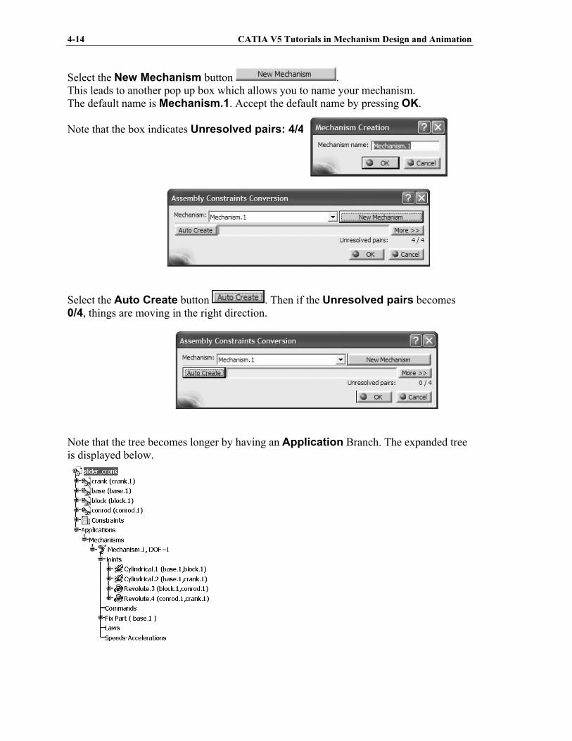
Select the New Mechanism button . This leads to another pop up box which allows you to name your mechanism. The default name is Mechanism.1. Accept the default name by pressing OK. Note that the box indicates Unresolved pairs: 4/4.
Select the Auto Create button . Then if the Unresolved pairs becomes 0/4, things are moving in the right direction.
Note that the tree becomes longer by having an Application Branch. The expanded tree is displayed below.
Slider Crank Mechanism 4-15
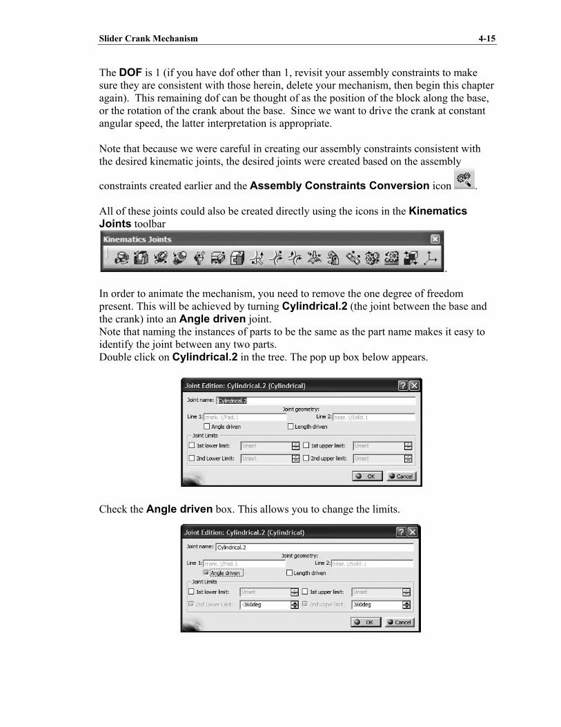
The DOF is 1 (if you have dof other than 1, revisit your assembly constraints to make sure they are consistent with those herein, delete your mechanism, then begin this chapter again). This remaining dof can be thought of as the position of the block along the base, or the rotation of the crank about the base. Since we want to drive the crank at constant angular speed, the latter interpretation is appropriate. Note that because we were careful in creating our assembly constraints consistent with the desired kinematic joints, the desired joints were created based on the assembly
constraints created earlier and the Assembly Constraints Conversion icon . All of these joints could also be created directly using the icons in the Kinematics Joints toolbar
. In order to animate the mechanism, you need to remove the one degree of freedom present. This will be achieved by turning Cylindrical.2 (the joint between the base and the crank) into an Angle driven joint. Note that naming the instances of parts to be the same as the part name makes it easy to identify the joint between any two parts. Double click on Cylindrical.2 in the tree. The pop up box below appears. Check the Angle driven box. This allows you to change the limits.

4-16 CATIA V5 Tutorials in Mechanism Design and Animation
Change the value of 2nd Lower Limit to be 0. Upon closing the above box and assuming that everything else was done correctly, the following message appears on the screen. This indeed is good news. According to CATIA V5 terminology, specifying Cylindrical.2 as an Angle driven joint is synonymous to defining a command. This is observed by the creation of Command.1 line in the tree.

Slider Crank Mechanism 4-17
We will now simulate the motion without regard to time based angular velocity. Select
the Simulation icon from the DMU Generic Animation toolbar
. This enables you to choose the mechanism to be animated if there are several present. In this case, select Mechanism.1 and close the window. As soon as the window is closed, a Simulation branch is added to the tree. As you scroll the bar in this toolbar from left to right, the crank begins to turn and makes a full 360 degree revolution. Notice that the zero position is simply the initial position of the assembly when the joint was created. Thus, if a particular zero position had been desired, a temporary assembly constraint could have been created earlier to locate the mechanism to the desired zero position. This temporary constraint would need to be deleted before conversion to mechanism joints.
4-18 CATIA V5 Tutorials in Mechanism Design and Animation
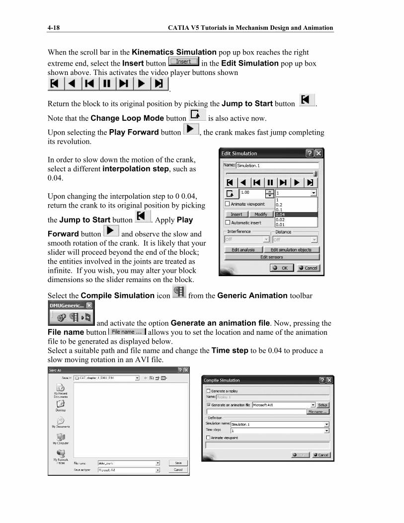
When the scroll bar in the Kinematics Simulation pop up box reaches the right
extreme end, select the Insert button in the Edit Simulation pop up box shown above. This activates the video player buttons shown
.
Return the block to its original position by picking the Jump to Start button .
Note that the Change Loop Mode button is also active now.
Upon selecting the Play Forward button , the crank makes fast jump completing its revolution. In order to slow down the motion of the crank, select a different interpolation step, such as 0.04. Upon changing the interpolation step to 0 0.04, return the crank to its original position by picking
the Jump to Start button . Apply Play
Forward button and observe the slow and smooth rotation of the crank. It is likely that your slider will proceed beyond the end of the block; the entities involved in the joints are treated as infinite. If you wish, you may alter your block dimensions so the slider remains on the block.
Select the Compile Simulation icon from the Generic Animation toolbar
and activate the option Generate an animation file. Now, pressing the File name button allows you to set the location and name of the animation file to be generated as displayed below. Select a suitable path and file name and change the Time step to be 0.04 to produce a slow moving rotation in an AVI file.
Slider Crank Mechanism 4-19
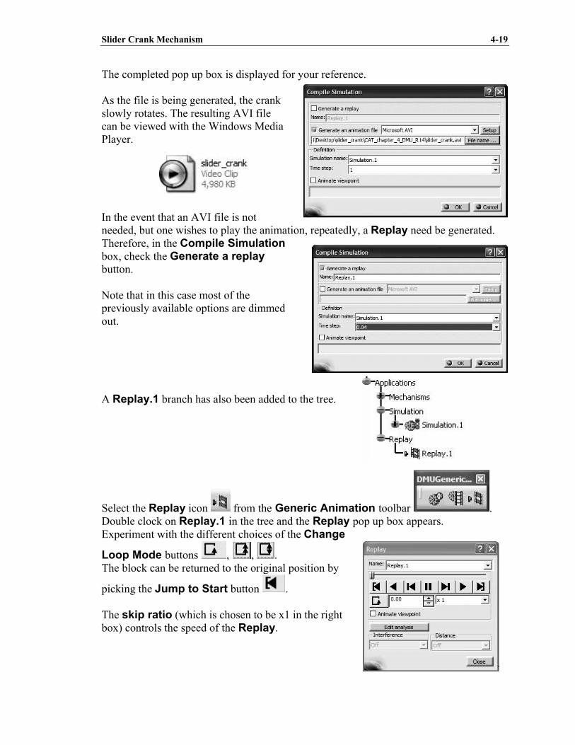
The completed pop up box is displayed for your reference. As the file is being generated, the crank slowly rotates. The resulting AVI file can be viewed with the Windows Media Player. In the event that an AVI file is not needed, but one wishes to play the animation, repeatedly, a Replay need be generated. Therefore, in the Compile Simulation box, check the Generate a replay button. Note that in this case most of the previously available options are dimmed out. A Replay.1 branch has also been added to the tree.
Select the Replay icon from the Generic Animation toolbar . Double clock on Replay.1 in the tree and the Replay pop up box appears. Experiment with the different choices of the Change
Loop Mode buttons , , . The block can be returned to the original position by
picking the Jump to Start button . The skip ratio (which is chosen to be x1 in the right box) controls the speed of the Replay.

4-20 CATIA V5 Tutorials in Mechanism Design and Animation
Once a Replay is generated such as Replay.1 in the tree above, it can also be played with a different icon.
Select the Simulation Player icon from the DMUPlayer toolbar . The outcome is the pop up box above. Use the cursor to pick Replay.1 from the tree.
The player keys are no longer dimmed out. Use the Play Forward (Right) button to begin the replay.
Slider Crank Mechanism 4-21
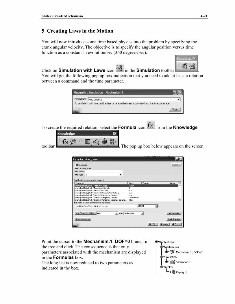
5 Creating Laws in the Motion You will now introduce some time based physics into the problem by specifying the crank angular velocity. The objective is to specify the angular position versus time function as a constant 1 revolution/sec (360 degrees/sec).
Click on Simulation with Laws icon in the Simulation toolbar . You will get the following pop up box indication that you need to add at least a relation between a command and the time parameter.
To create the required relation, select the Formula icon from the Knowledge
toolbar . The pop up box below appears on the screen. Point the cursor to the Mechanism.1, DOF=0 branch in the tree and click. The consequence is that only parameters associated with the mechanism are displayed in the Formulas box. The long list is now reduced to two parameters as indicated in the box.

4-22 CATIA V5 Tutorials in Mechanism Design and Animation
Select the entry Mechanism.1\Commands\Command.1\Angle and press the Add
Formula button . This action kicks you to the Formula Editor box. Pick the Time entry from the middle column (i.e., Members of Parameters) then double click on Mechanism.1\KINTime in the Members of Time column.
Slider Crank Mechanism 4-23
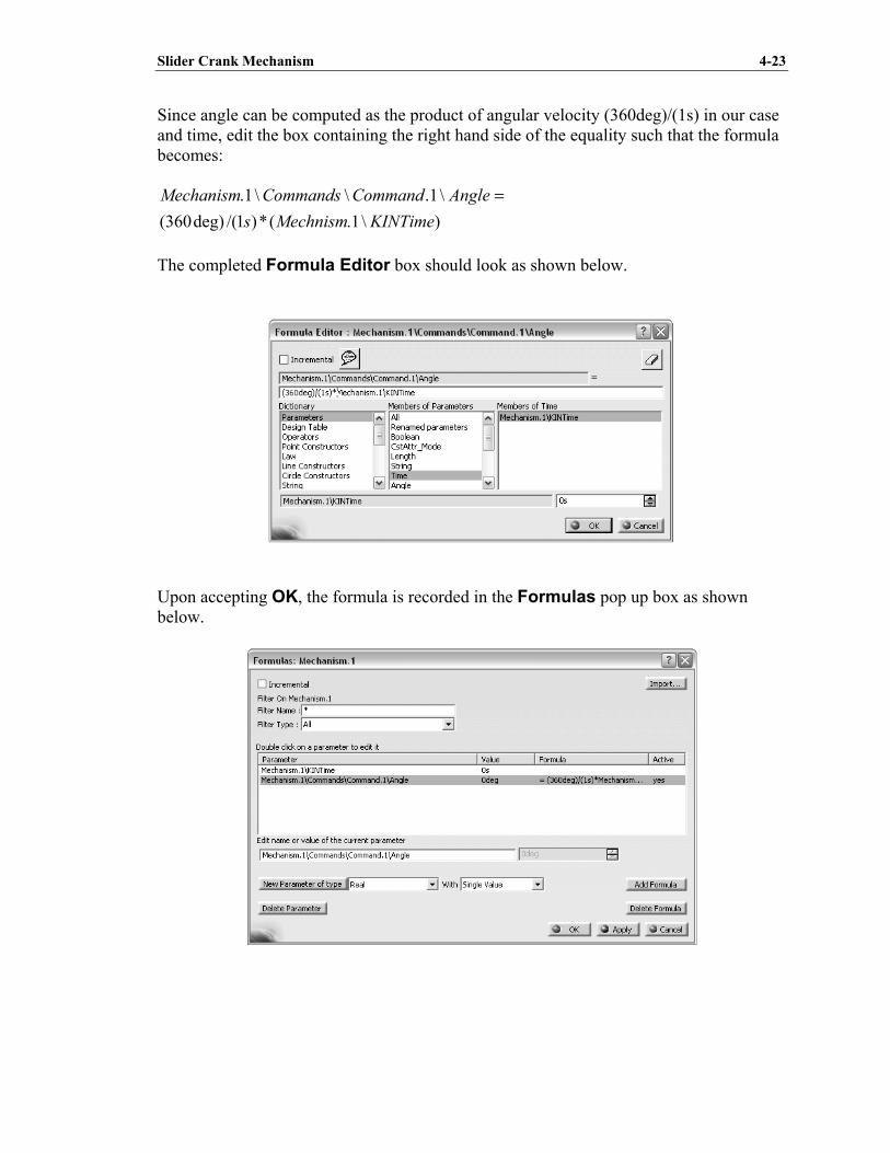
Since angle can be computed as the product of angular velocity (360deg)/(1s) in our case and time, edit the box containing the right hand side of the equality such that the formula becomes:
)\1.(*)1/(deg)360(
\1.\\1.
KINTimeMechnismsAngleCommandCommandsMechanism =
The completed Formula Editor box should look as shown below.
Upon accepting OK, the formula is recorded in the Formulas pop up box as shown below.

4-24 CATIA V5 Tutorials in Mechanism Design and Animation
Careful attention must be given to the units when writing formulas involving the kinematic parameters. In the event that the formula has different units at the different sides of the equality you will get Warning messages such as the one shown below. We are spared the warning message because the formula has been properly inputted. Note that the introduced law has appeared in Law branch of the tree. Keep in mind that our interest is to plot the position, velocity and accelerations generated
by this motion. To set this up, select the Speed and Acceleration icon from the
DMU Kinematics toolbar . The pop up box below appears on the Screen. For the Reference product, select the base from the screen or the tree. For the Point selection, pick the vertex of the block as shown in the sketch below. This will set up the sensor to record the movement of the chosen point relative to the base (which is fixed).

Slider Crank Mechanism 4-25
Note that the Speed and Acceleration.1 has appeared in the tree.
Having entered the required kinematic relation and designated the vertex on the block as the point to collect data on, we will simulate the mechanism. Click on Simulation with
Laws icon in the Simulation toolbar . This results in the Kinematics Simulation pop up box shown below. Note that the default time duration is 10 seconds. To change this value, click on the button
. In the resulting pop up box, change the time duration to 1s. This is the time duration for the crank to make one full revolution.
For Reference product, pick the base
For Point selection, pick this vertex
For Reference product, pick the base
For Point selection, pick this vertex

4-26 CATIA V5 Tutorials in Mechanism Design and Animation
The scroll bar now moves up to 1s. Check the Activate sensors box, at the bottom left corner. (Note: CATIA V5R15 users will also see a Plot vectors box in this window). You will next have to make certain selections from the accompanying Sensors box. Observing that the coordinate direction of interest is X, click on the following items to record position, velocity, and acceleration of the block: Mechanism.1\Joints\Cylindrical.1\Length Speed-Acceleration.1\X_LinearSpeed Speed-Acceleration.1\X_LinearAcceleration As you make selections in this window, the last column in the Sensors box, changes to Yes for the corresponding items. This is shown on the next page. Do not close the Sensors box after you have made your selection (leave it open to generate results).

Slider Crank Mechanism 4-27
The larger this number,The smoother the plotsThe larger this number,The smoother the plots
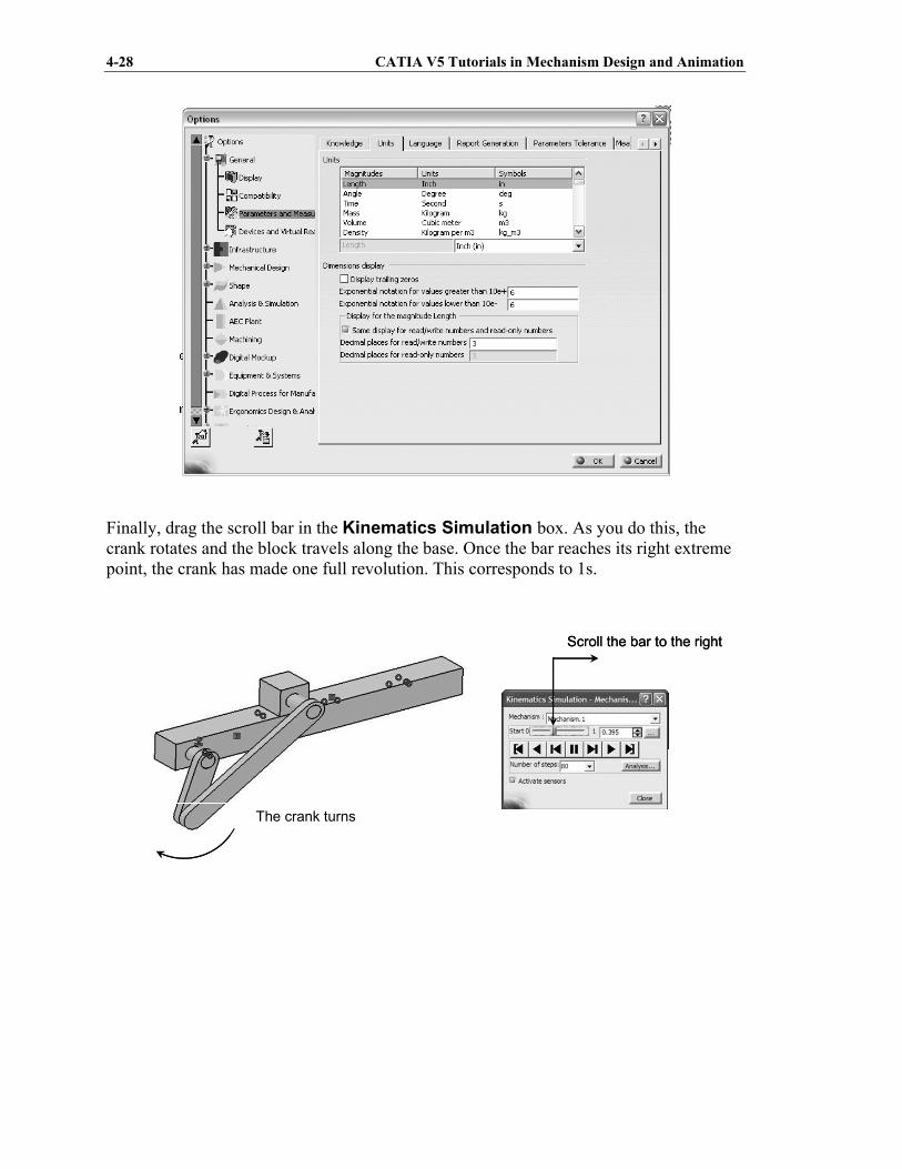
Also, change the Number of steps to 80. The larger this number, the smoother the velocity and acceleration plots will be. Note: If you haven’t already done so, change the default units on position, velocity and acceleration to in, in/s and in/s2, respectively. This is done in the Tools, Options, Parameters and Measures menu shown on the next page.
4-28 CATIA V5 Tutorials in Mechanism Design and Animation
Finally, drag the scroll bar in the Kinematics Simulation box. As you do this, the crank rotates and the block travels along the base. Once the bar reaches its right extreme point, the crank has made one full revolution. This corresponds to 1s.
Scroll the bar to the rightScroll the bar to the right
The crank turnsThe crank turns
Slider Crank Mechanism 4-29
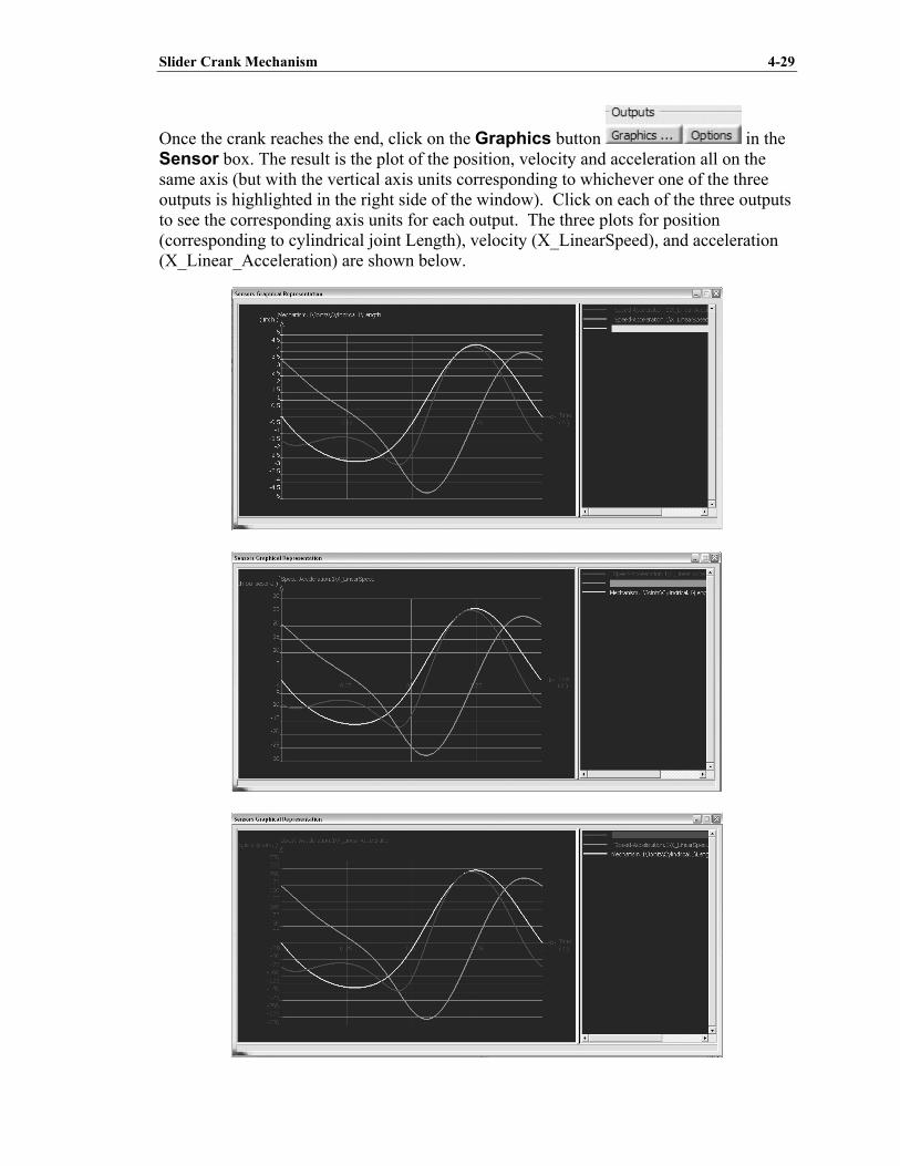
Once the crank reaches the end, click on the Graphics button in the Sensor box. The result is the plot of the position, velocity and acceleration all on the same axis (but with the vertical axis units corresponding to whichever one of the three outputs is highlighted in the right side of the window). Click on each of the three outputs to see the corresponding axis units for each output. The three plots for position (corresponding to cylindrical joint Length), velocity (X_LinearSpeed), and acceleration (X_Linear_Acceleration) are shown below.
4-30 CATIA V5 Tutorials in Mechanism Design and Animation
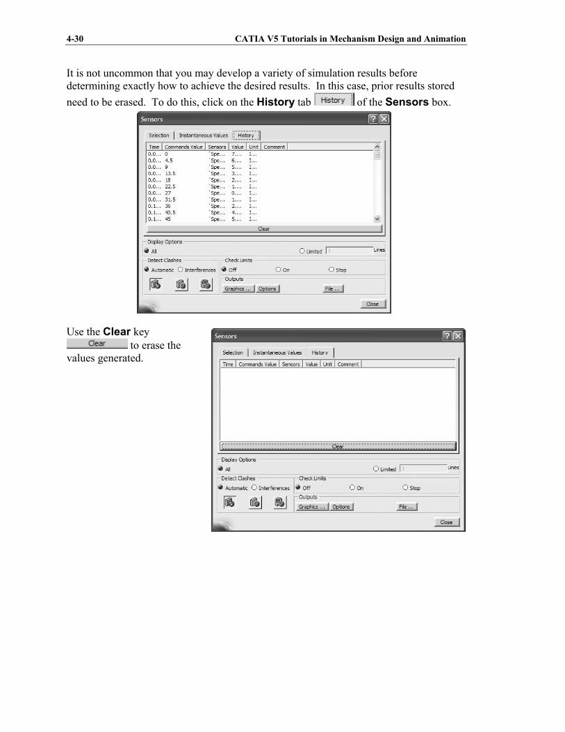
It is not uncommon that you may develop a variety of simulation results before determining exactly how to achieve the desired results. In this case, prior results stored
need to be erased. To do this, click on the History tab of the Sensors box. Use the Clear key
to erase the values generated.

Slider Crank Mechanism 4-31
Next, we will create a plot which is not simply versus time. As an illustrative example, we will place a point somewhere along the conrod. For this point, we will plot its linear speed and linear acceleration versus crank angle. It is important to note that DMU computes positive scalars for linear speeds and linear accelerations since it simply computes the magnitude based on the three rectangular components. First, return to Part Design and create a reference point on the conrod at the approximate location as shown below. Return to DMU. The plan is to generate two plots. The first plot is the speed of the created point against the angular position of the crank. The second plot is the acceleration of the created point against the angular position of the crank. In order to generate the speed and acceleration data, you need to use the Speed and
Acceleration icon from the DMU Kinematics toolbar
. Click on the icon and in the resulting pop up box make the following selections. For Reference product, pick the base from the screen. For Reference point, pick the point that was created earlier on the conrod.
x
Create a point on theconrod approximately at this location
x
Create a point on theconrod approximately at this location
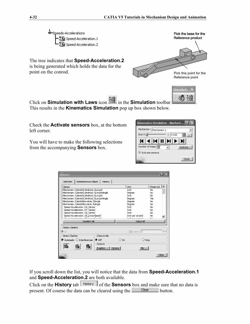
4-32 CATIA V5 Tutorials in Mechanism Design and Animation
x
Pick this point for theReference point
Pick the base for theReference product
x
Pick this point for theReference point
Pick the base for theReference product
The tree indicates that Speed-Acceleration.2 is being generated which holds the data for the point on the conrod.
Click on Simulation with Laws icon in the Simulation toolbar . This results in the Kinematics Simulation pop up box shown below. Check the Activate sensors box, at the bottom left corner. You will have to make the following selections from the accompanying Sensors box. If you scroll down the list, you will notice that the data from Speed-Acceleration.1 and Speed-Acceleration.2 are both available.
Click on the History tab of the Sensors box and make sure that no data is present. Of course the data can be cleared using the button.
Slider Crank Mechanism 4-33
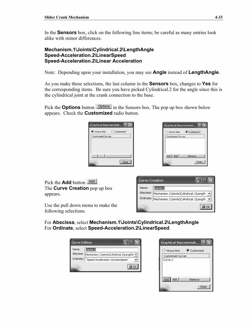
In the Sensors box, click on the following line items; be careful as many entries look alike with minor differences. Mechanism.1\Joints\Cylindrical.2\LengthAngle Speed-Acceleration.2\LinearSpeed Speed-Acceleration.2\Linear Acceleration Note: Depending upon your installation, you may see Angle instead of LengthAngle. As you make these selections, the last column in the Sensors box, changes to Yes for the corresponding items. Be sure you have picked Cylindrical.2 for the angle since this is the cylindrical joint at the crank connection to the base. Pick the Options button in the Sensors box. The pop up box shown below appears. Check the Customized radio button.
Pick the Add button . The Curve Creation pop up box appears. Use the pull down menu to make the following selections. For Abscissa, select Mechanism.1\Joints\Cylindrical.2\LengthAngle For Ordinate, select Speed-Acceleration.2\LinearSpeed.
4-34 CATIA V5 Tutorials in Mechanism Design and Animation
Drag the scroll bar allthe way to the rightor simply click on
Drag the scroll bar allthe way to the rightor simply click on
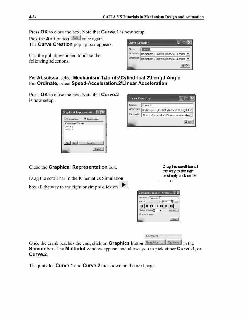
Press OK to close the box. Note that Curve.1 is now setup.
Pick the Add button once again. The Curve Creation pop up box appears. Use the pull down menu to make the following selections. For Abscissa, select Mechanism.1\Joints\Cylindrical.2\LengthAngle For Ordinate, select Speed-Acceleration.2\Linear Acceleration Press OK to close the box. Note that Curve.2 is now setup. Close the Graphical Representation box. Drag the scroll bar in the Kinematics Simulation
box all the way to the right or simply click on .
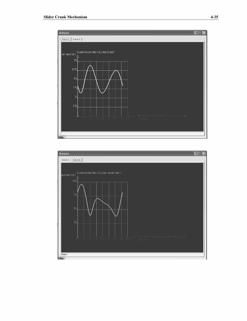
Once the crank reaches the end, click on Graphics button in the Sensor box. The Multiplot window appears and allows you to pick either Curve.1, or Curve.2. The plots for Curve.1 and Curve.2 are shown on the next page.
Slider Crank Mechanism 4-35