A 3D Modeling System based onPolar Meshes

Daniele Brazzolotto

Kongens Lyngby 2013

COMPUTE-M.Sc-2013-63

Supervisors:

DTU: J. Andreas Bærenten - janba@dtu.dk

Padova: Giovanni De Poli - depoli@dei.unipd.it

Technical University of DenmarkApplied Mathematics and Computer ScienceBuilding 303B, DK-2800 Kongens Lyngby, DenmarkPhone +45 4525 3031, Fax +45 4588 1399compute@compute.dtu.dkwww.compute.dtu.dk Compute-M.Sc-2013-63

Summary (English)

In 3D multimedia productions, modeling is an activity that absorbs a considerableamount of e�ort and during the years it has been the focus of an entire line ofresearch. This research �eld includes SQM, a method originally developed by J.A. Bærentzen, M. K. Misztal and K. Welnicka [JAB12], where the �nal mesh isprocedurally inferred from the skeleton that the designer has modeled. It turnedout to be a great tool to quickly de�ne the high level structure of the object but itis strongly limited in terms of mesh details, the exact opposite of a traditional 3Dtool.

This project aims to design a new modeling system that merges the bene�ts ofSQM with the strengths of a traditional sculpturing tool, recognizing the needs fortwo di�erent modeling levels: at high level, polar meshes have been used to quicklyde�ne the structure of the object, while at low level the designer is free to add meshdetails like in any other 3D application.

In this thesis a core set of polar mesh operations have been de�ned and implementedin a small modeling prototype. On top of that, it has also been developed a behaviorbased animation engine and an L-System, to evaluate the bene�ts that a modelingsystem based on polar meshes can o�er to these areas.

The new modeling system pushes the production of 3D assets towards a more AGILEprocess, it can procedurally recognize and generate the mesh skeleton and it naivelysupports structure based operations, including morphing, bottom-up animations andprocedurally generated content.

ii

Summary (Italian)

Nella produzione di contenuti multimediali, la modellazione di asset 3D è un'attivitàche richiede una consistente porzione del costo complessivo di sviluppo ed è al cen-tro di un intero �lone di ricerca che include SQM, un metodo sviluppato da J.A. Bærentzen, M. K. Misztal e K. Welnicka [JAB12] in cui la mesh viene auto-maticamente generata dall'ossatura indicata dal designer. Si tratta di un metodoestremamente e�cace per de�nire la struttura ad alto livello del modello, ma che èanche fortemente limitato per quanto riguarda i particolari che è possibile aggiungerealla mesh stessa, l'esatto opposto del tipico software di modellazione tradizionale.

L'obiettivo di questo lavoro è la progettazione di un sistema di modellazione che siain grado di unire i vantaggi di SQM con i punti di forza dei tradizionali software3D, riconoscendo la necessità di due distinti livelli operativi: ad alto livello verrannosfruttate le proprietà delle mesh polari per de�nire la struttura di base dell'oggetto,mentre a basso livello il designer sarà libero di aggiungere particolari alla mesh comein ogni altro software 3D.

In questa tesi sono state progettate un insieme di operazioni per mesh polari, poiimplementate in un piccolo tool di modellazione. E' stato inoltre sviluppato unmotore di animazione comportamentale e un L-System per valutare i bene�ci cheun sistema di modellazione basato su mesh polari può o�rire anche in riferimento aquesti ambiti.

Il nuovo sistema di modellazione spinge la produzione di elementi 3D verso unprocesso di sviluppo più AGILE, è in grado di generare automaticamente la strutturadella mesh e supporta nativamente operazioni come morphing, animationi bottom-up e la generazione automatica di asset multimediali.

iv

Preface

This thesis was prepared at DTU Compute, Department of Applied Mathematicsand Computer Science at the Technical University of Denmark in ful�llment of therequirements for acquiring a M.Sc. in Digital Media Engineering as well as a M.Sc.in Computer Engineering, respectively at the Technical University of Denmark andat the University of Padova, according to the bilateral agreements that regulate thecollaboration between these institutions in the frame of the T.I.M.E. double degreeprogram (https://www.time-association.org/).

This project represents an evolution of the SQM method which has been originallydeveloped by J. A. Bærentzen, M. K. Misztal and K. Welnicka [JAB12] and thathas been later analyzed and extended by Michael Mc Donnell [Don12]. SQM is partof a more general line of research that aims to provide a better support for 3D meshmanipulation not only from the point of view of modeling but also for animationsand procedurally generated content. In this framework, more abstract tools cancontribute to reduce the cost of 3D digital assets, increasing the productivity ofdesigners and animators.

In his thesis, Mc Donnell proved that SQM is a�ected by severe limitations whenthe object which needs to be modeled is inorganic or it hasn't a clear structure.These limitations are more an intrinsic characteristic of the modeling system ratherthan a consequence of the limited set of node types of the original SQM method.

This project proposes a new modeling system, based on the same mesh topologythat characterizes SQM, but it has been developed from a completely di�erent setof principles: the mesh is a numerical approximation of the smooth surface thatthe designer wants to model, it includes structural information regarding the objectwhich has been represented as well as surface details, but de�ning what is structure

vi

and what is detail is a pure design choice. An e�ective modeling system maintainsa balance between those two layers and it supports both of them with di�erent,although integrated, sets of mesh tools.

The modeling system that will be presented in this report is the result of an iterativeprocess that has rede�ned multiple times the characteristics of the desired tool, ledby a progressively deeper understanding of the of the mesh topology which ultimatelyhas a�ected also the concept of polar mesh itself.

This thesis doesn't provide a complete modeling tool, neither it is an exhaustiveexploration of opportunities and limitations o�ered by this approach, but it doesprovide an overview of the potential that a modeling system based on polar meshescan o�er. In this perspective this project yielded a positive outcome, it is de�nitelya proof of concept that motivates further developments, both academically andcommercially, and there are the basics for a �rst integration with existing productiontools.

Lyngby, 15-July-2013

Daniele Brazzolotto

daniele.brazzolotto@gmail.comhttp://linkedin.com/in/danielebrazzolotto

Acknowledgments

First of all I would like to thank my family for its constant support since the verybeginning of my Danish adventure, when I decided to apply for this double degreeprogram. The last two years represented an incredible opportunity to grow uppersonally and professionally in a way that I couldn't have imagined before. I'mthankful to them all for giving me this opportunity and for supporting me throughoutthe challenges that characterized this intense period of my life.

I would also like to thank my supervisor J. A. Bærentzen for his assistance duringall the phases of this thesis work as well as for providing the GEL framework, whichconsiderably simpli�ed the technical implementation of the prototype. I show my ap-preciation to DTU-Compute for hosting this project and speci�cally to Jeppe RevallFrisvad for providing, together with J. A. Bærentzen, weekly feedback throughoutthe entire working process.

As double degree T.I.M.E. student (https://www.time-association.org/), I wouldlike to show my appreciation to my italian supervisor Giovanni De Poli for hissupport and �nally I would like to thank the Technical University of Denmark andthe University of Padova, I'm grateful to whoever in these institutions maintainsand improves the T.I.M.E network, promoting the mutual academic recognition.

viii Contents

Contents

Summary (English) i

Summary (Italian) iii

Preface v

Acknowledgments vii

1 Introduction 11.1 Prerequisites . . . . . . . . . . . . . . . . . . . . . . . . . . . . . . 11.2 Purposes . . . . . . . . . . . . . . . . . . . . . . . . . . . . . . . 21.3 Expected outcomes . . . . . . . . . . . . . . . . . . . . . . . . . . 4

1.3.1 Faster modeling . . . . . . . . . . . . . . . . . . . . . . . . 41.3.2 Agile modeling . . . . . . . . . . . . . . . . . . . . . . . . 41.3.3 Animations . . . . . . . . . . . . . . . . . . . . . . . . . . 51.3.4 Procedurally generated content . . . . . . . . . . . . . . . . 6

1.4 The project . . . . . . . . . . . . . . . . . . . . . . . . . . . . . . 6

I Modeling 9

2 A new modeling system 112.1 Concept of polar mesh . . . . . . . . . . . . . . . . . . . . . . . . 112.2 SQM: Skeleton to Quad Mesh . . . . . . . . . . . . . . . . . . . . 122.3 This project as an evolution of SQM . . . . . . . . . . . . . . . . . 142.4 The new modeling system . . . . . . . . . . . . . . . . . . . . . . . 152.5 Consideration on mesh topology . . . . . . . . . . . . . . . . . . . 16

2.5.1 Triangles vs Quad dominant meshes . . . . . . . . . . . . . 162.5.2 Polar meshes from a topology prospective . . . . . . . . . . 17

x CONTENTS

3 Polar Meshes 193.1 Notation . . . . . . . . . . . . . . . . . . . . . . . . . . . . . . . . 20

3.1.1 Mesh elements . . . . . . . . . . . . . . . . . . . . . . . . . 213.1.2 Properties of mesh elements . . . . . . . . . . . . . . . . . 213.1.3 Basic mesh navigation . . . . . . . . . . . . . . . . . . . . . 213.1.4 Basic mesh operations . . . . . . . . . . . . . . . . . . . . . 22

3.2 Topological Properties . . . . . . . . . . . . . . . . . . . . . . . . . 223.2.1 Poles arbitrariness . . . . . . . . . . . . . . . . . . . . . . . 223.2.2 Loops arbitrariness . . . . . . . . . . . . . . . . . . . . . . 233.2.3 Loop and backbone connectivity . . . . . . . . . . . . . . . 24

3.3 Iterators . . . . . . . . . . . . . . . . . . . . . . . . . . . . . . . . 243.3.1 Loop iterator . . . . . . . . . . . . . . . . . . . . . . . . . 243.3.2 Parallel iterator . . . . . . . . . . . . . . . . . . . . . . . . 253.3.3 Fan iterator . . . . . . . . . . . . . . . . . . . . . . . . . . 25

3.4 Features . . . . . . . . . . . . . . . . . . . . . . . . . . . . . . . . 253.4.1 De�nitions . . . . . . . . . . . . . . . . . . . . . . . . . . . 253.4.2 Child features . . . . . . . . . . . . . . . . . . . . . . . . . 26

4 Core Operations 274.1 Add re�nement . . . . . . . . . . . . . . . . . . . . . . . . . . . . 27

4.1.1 Speci�cation . . . . . . . . . . . . . . . . . . . . . . . . . . 274.1.2 Implementation . . . . . . . . . . . . . . . . . . . . . . . . 284.1.3 Description . . . . . . . . . . . . . . . . . . . . . . . . . . 284.1.4 Limitations . . . . . . . . . . . . . . . . . . . . . . . . . . . 29

4.2 Remove re�nement . . . . . . . . . . . . . . . . . . . . . . . . . . 294.2.1 Speci�cation . . . . . . . . . . . . . . . . . . . . . . . . . . 294.2.2 Implementation . . . . . . . . . . . . . . . . . . . . . . . . 304.2.3 Description . . . . . . . . . . . . . . . . . . . . . . . . . . 304.2.4 Limitations . . . . . . . . . . . . . . . . . . . . . . . . . . . 30

4.3 Add Feature . . . . . . . . . . . . . . . . . . . . . . . . . . . . . . 314.3.1 Speci�cation . . . . . . . . . . . . . . . . . . . . . . . . . . 314.3.2 Implementation . . . . . . . . . . . . . . . . . . . . . . . . 324.3.3 Description . . . . . . . . . . . . . . . . . . . . . . . . . . 324.3.4 Limitations . . . . . . . . . . . . . . . . . . . . . . . . . . . 33

4.4 Select Feature . . . . . . . . . . . . . . . . . . . . . . . . . . . . . 334.4.1 Speci�cation . . . . . . . . . . . . . . . . . . . . . . . . . . 334.4.2 Implementation . . . . . . . . . . . . . . . . . . . . . . . . 344.4.3 Description . . . . . . . . . . . . . . . . . . . . . . . . . . 34

4.5 Remove Feature . . . . . . . . . . . . . . . . . . . . . . . . . . . . 354.5.1 Speci�cation . . . . . . . . . . . . . . . . . . . . . . . . . . 354.5.2 Implementation . . . . . . . . . . . . . . . . . . . . . . . . 354.5.3 Description . . . . . . . . . . . . . . . . . . . . . . . . . . 374.5.4 Limitations . . . . . . . . . . . . . . . . . . . . . . . . . . . 37

4.6 Merge Features . . . . . . . . . . . . . . . . . . . . . . . . . . . . 39

CONTENTS xi

4.6.1 Speci�cation . . . . . . . . . . . . . . . . . . . . . . . . . . 39

4.6.2 Implementation . . . . . . . . . . . . . . . . . . . . . . . . 39

4.6.3 Description . . . . . . . . . . . . . . . . . . . . . . . . . . 40

4.6.4 Limitations . . . . . . . . . . . . . . . . . . . . . . . . . . . 40

4.7 Split Feature . . . . . . . . . . . . . . . . . . . . . . . . . . . . . . 40

4.7.1 Speci�cation . . . . . . . . . . . . . . . . . . . . . . . . . . 40

4.7.2 Implementation . . . . . . . . . . . . . . . . . . . . . . . . 41

4.7.3 Description . . . . . . . . . . . . . . . . . . . . . . . . . . 41

4.8 Example . . . . . . . . . . . . . . . . . . . . . . . . . . . . . . . . 42

5 Analysis 47

5.1 Lollipop . . . . . . . . . . . . . . . . . . . . . . . . . . . . . . . . 48

5.2 Gear . . . . . . . . . . . . . . . . . . . . . . . . . . . . . . . . . . 49

5.3 Ladder . . . . . . . . . . . . . . . . . . . . . . . . . . . . . . . . . 51

5.4 Head . . . . . . . . . . . . . . . . . . . . . . . . . . . . . . . . . . 52

5.5 Conclusions . . . . . . . . . . . . . . . . . . . . . . . . . . . . . . 54

II Animation 57

6 Animation engines 59

6.1 Animation description . . . . . . . . . . . . . . . . . . . . . . . . . 60

6.2 Animation engines . . . . . . . . . . . . . . . . . . . . . . . . . . . 61

7 Animation of polar meshes 63

7.1 Inferring the skeleton . . . . . . . . . . . . . . . . . . . . . . . . . 63

7.1.1 Relative root node . . . . . . . . . . . . . . . . . . . . . . . 65

7.1.2 Examples . . . . . . . . . . . . . . . . . . . . . . . . . . . 65

7.2 Skeleton based coordinates . . . . . . . . . . . . . . . . . . . . . . 67

7.3 Skinning of polar meshes . . . . . . . . . . . . . . . . . . . . . . . 67

8 Implementation 71

8.1 The prototype . . . . . . . . . . . . . . . . . . . . . . . . . . . . . 71

9 Analysis 75

9.1 Morphing . . . . . . . . . . . . . . . . . . . . . . . . . . . . . . . . 75

9.2 Gravity . . . . . . . . . . . . . . . . . . . . . . . . . . . . . . . . . 78

9.2.1 Mathematical model . . . . . . . . . . . . . . . . . . . . . 79

9.2.2 Constrains of skeleton structure . . . . . . . . . . . . . . . 80

9.2.3 Rendering . . . . . . . . . . . . . . . . . . . . . . . . . . . 80

9.3 Morphing and Gravity combined . . . . . . . . . . . . . . . . . . . 81

9.4 Conclusions . . . . . . . . . . . . . . . . . . . . . . . . . . . . . . 81

xii CONTENTS

III Procedurally generated content 85

10 L-Systems 8710.1 Introduction to L-Systems . . . . . . . . . . . . . . . . . . . . . . . 8710.2 Classes of L-Systems . . . . . . . . . . . . . . . . . . . . . . . . . 8810.3 Turtle representation of L-System . . . . . . . . . . . . . . . . . . . 8910.4 L-System and polar meshes . . . . . . . . . . . . . . . . . . . . . . 91

11 Implementation 9311.1 Implicit string representation and real time mesh operations . . . . . 95

12 Analysis 97

IV Conclusions 101

13 Conclusions 103

14 Further Work 107

V Appendices 109

A Project management 111A.1 Development process . . . . . . . . . . . . . . . . . . . . . . . . . 111A.2 Risk analysis . . . . . . . . . . . . . . . . . . . . . . . . . . . . . . 113

B Prototype 115B.1 The shader . . . . . . . . . . . . . . . . . . . . . . . . . . . . . . . 115

B.1.1 Basic di�use shader . . . . . . . . . . . . . . . . . . . . . . 116B.1.2 Geometry shader and wireframe . . . . . . . . . . . . . . . 116B.1.3 Color coded information . . . . . . . . . . . . . . . . . . . . 117

C Animation techniques 119C.1 Keyframes . . . . . . . . . . . . . . . . . . . . . . . . . . . . . . . 119C.2 Animation scripting languages . . . . . . . . . . . . . . . . . . . . 120C.3 Goal oriented motion . . . . . . . . . . . . . . . . . . . . . . . . . 121C.4 Motion capture . . . . . . . . . . . . . . . . . . . . . . . . . . . . 122

Chapter 1

Introduction

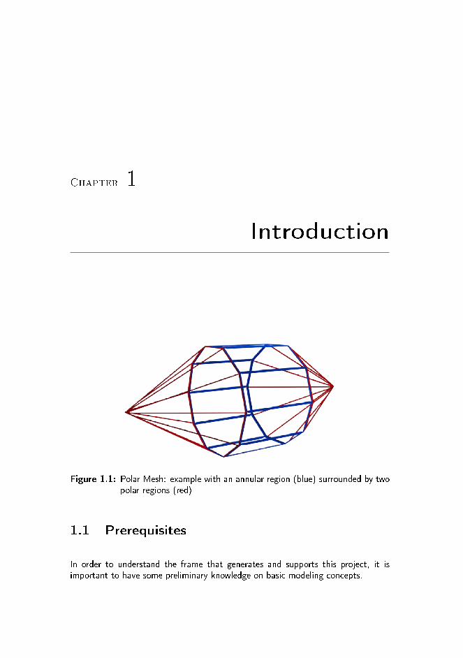
Figure 1.1: Polar Mesh: example with an annular region (blue) surrounded by twopolar regions (red)

1.1 Prerequisites

In order to understand the frame that generates and supports this project, it isimportant to have some preliminary knowledge on basic modeling concepts.

2 Introduction

The core of this thesis is the development of a modeling system, a collection oftechnologies, tools and techniques that designers can use to produce 3D assets. Inother words a modeling system is the set of principles that are at the base of a 3Dmodeling software and which are indirectly shown through the operations that thetool makes available to the user.

A second key concept for this project is polar meshes, polygonal meshes charac-terized by a strictly regulated topology that supports the polar subdivision scheme[KP07b] and that can be seen as a collection of polar and annular regions [KP07a],or more informally as a collection of cones and cylinders (�gure 1.1).

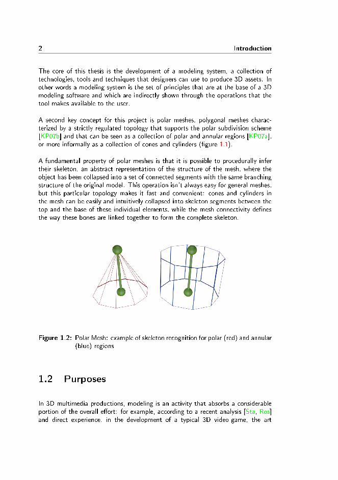
A fundamental property of polar meshes is that it is possible to procedurally infertheir skeleton, an abstract representation of the structure of the mesh, where theobject has been collapsed into a set of connected segments with the same branchingstructure of the original model. This operation isn't always easy for general meshes,but this particular topology makes it fast and convenient: cones and cylinders inthe mesh can be easily and intuitively collapsed into skeleton segments between thetop and the base of these individual elements, while the mesh connectivity de�nesthe way these bones are linked together to form the complete skeleton.

Figure 1.2: Polar Mesh: example of skeleton recognition for polar (red) and annular(blue) regions

1.2 Purposes

In 3D multimedia productions, modeling is an activity that absorbs a considerableportion of the overall e�ort: for example, according to a recent analysis [Sta, Ros]and direct experience, in the development of a typical 3D video-game, the art

1.2 Purposes 3

department absorbs 40% to 75% of the entire production manpower. Modeling,rigging1 and texturing2 the few organic objects requires 60% to 90% of the resourcesof the art team and it a�ects 30% to 65% of the entire production cost. Thereforea 30% optimization of the modeling phase will directly reduce the production costof 10% - 20%.

This project is part of a more general line of research that aims to speed-up andsimplify the modeling of complex objects, providing a better support for 3D meshmanipulation. In this work, this goal will be reached de�ning and implementinga set of mesh operations that will positively a�ect the modeling phase as well asanimations and procedurally generated content.

Nowadays the main problem with 3D modeling is the low level of abstraction: mostof the 3D tools allow the designers to work with vertices and faces, but nothingmore than that. It is like to construct a building with bricks and mortar: it surelycan be done, but prefabricated components can make the work faster, cheaper andeasier.

The idea behind this thesis is to exploit some of the characteristics of polar meshesto give to designers the right tools to build and use the virtual equivalents ofprefabricated concrete components:

Skeleton: every polar mesh has an implicit skeleton, that can be procedurally in-ferred run time. This isn't only suitable to automatically generate a bonestructure for future animations, but it is also a way to group vertices andfaces together. This is a �rst abstraction level to design operations thata�ect several faces at once in a meaningful and coherent way.

Features: in a typical polar mesh, most of the skeleton segments are simply placedin a line, without any branching. A consecutive, connected sequence of skele-ton segments can be grouped in a feature. This is a second important ab-straction level for interesting mesh operations, that get closer to how humanbrain gives meaning to things: if you look at �gure 1.3, you will have no doubtthat it is a little man thanks mainly to the branching structure of the lines.Mesh operations at feature level re�ect the way a designer thinks and meansand, for this reason, they can play an important role in tools that aim to bee�ective and easy to use.

1Rigging: http://en.wikipedia.org/wiki/Skeletal_animation2Texturing or texture mapping: http://en.wikipedia.org/wiki/Texture_mapping

4 Introduction

Figure 1.3: Stylized man: example of human brain's capability to recognize shapesbased on branching structure

1.3 Expected outcomes

The bene�ts of the improved modeling system and of the higher abstraction levelnot only cover di�erent areas of the 3D modeling pipeline but they are also thebasics for new real time techniques.

1.3.1 Faster modeling

A �rst important expected outcome is surely a faster modeling system: as it hasbeen previously discussed, modeling time can be signi�cantly reduced with featurebased tools and operations. This single improvement would be enough to justify theentire thesis work as it has a direct impact on the costs of most 3D productions.

1.3.2 Agile modeling

A lesson that every software developer quickly learns is that a software (or a digitalproduct in general) is always a unique piece. Probably a similar need can be requiredin the future, but the exact same need is very unlikely; therefore one can surely usea previous work, but it must be changed and customized to the new request.

This fuzzy concept of re-usage is well known in the world of software developmentas well as in some other areas, but unfortunately the production of 3D assets is farbehind on this process: ask a 3D artist to change the structure of a model and mostlikely he will start from scratch again.

Although the mainstream culture in the art department is still waterfall based ratherthan AGILE, it is also true that most of existing tools don't support approaches basedon re�nements and probably these two aspects are related.

A modeling system based on polar meshes can actually support an AGILE approach,

1.3 Expected outcomes 5

not only because the designer can step by step re�ne the mesh up to the desiredlevel of details, but also because there is an implicit skeleton that can be used toautomatically rig the mesh to the bones. The designer at this point is free to adjustand re�ne a completely animated character without compromising the entire riggingand animations already set up.

Moreover it is also possible to select entire features, to copy them into other modelsor to save them for later usage. This is the base of a new generation of objectlibraries, where the old copy-paste pattern is replaced by the more �exible recombine-customize: the upper body of an alien and the lower body of a humanoid can bemixed together, can be re�ned to adjust the mesh details and a complete newcharacter is served. Rigged, animated and textured for free.

Waterfall and AGILE development

Waterfall [Roy70] is a linear development process where the project follows a se-quential life cycle: the new development phase starts only when the previous hasbeen fully completed. This was the �rst method that has been applied to the devel-opment of digital products and it often leads to unbounded delays and incrementsof the production cost.

The antithesis of waterfall is AGILE [HF01], a term introduced in 2001 to group aclass of iterative and incremental development methods, where the digital productevolves in rapid cycles: in each iteration self organized and cross functional teamsexecute the entire production pipeline, from requirements speci�cation to releaseand consequently at the end of each cycle a working product is always available forreviews. The feedback that is possible to gain at the end of each iteration is animportant component of the AGILE method and it allows the team to start the newcycle with the most updated requirements.

The bene�ts of the AGILE approach has been largely proven in the software devel-opment world, but the same principles can be applied straight forward in almost anydigital production.

1.3.3 Animations

Some of the bene�ts of a mesh with an implicit skeleton is the animation system,which can be simpli�ed to support a more direct application of the standard IKtechnique.

Polar meshes provide also a good support to physically based behaviors, computedin real time using the structural information intrinsically embedded in the meshtopology: the global deformation can be implemented as a combination of localized

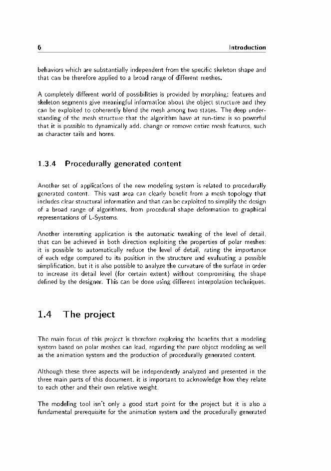
6 Introduction

behaviors which are substantially independent from the speci�c skeleton shape andthat can be therefore applied to a broad range of di�erent meshes.

A completely di�erent world of possibilities is provided by morphing: features andskeleton segments give meaningful information about the object structure and theycan be exploited to coherently blend the mesh among two states. The deep under-standing of the mesh structure that the algorithm have at run-time is so powerfulthat it is possible to dynamically add, change or remove entire mesh features, suchas character tails and horns.

1.3.4 Procedurally generated content

Another set of applications of the new modeling system is related to procedurallygenerated content. This vast area can clearly bene�t from a mesh topology thatincludes clear structural information and that can be exploited to simplify the designof a broad range of algorithms, from procedural shape deformation to graphicalrepresentations of L-Systems.

Another interesting application is the automatic tweaking of the level of detail,that can be achieved in both direction exploiting the properties of polar meshes:it is possible to automatically reduce the level of detail, rating the importanceof each edge compared to its position in the structure and evaluating a possiblesimpli�cation, but it is also possible to analyze the curvature of the surface in orderto increase its detail level (for certain extent) without compromising the shapede�ned by the designer. This can be done using di�erent interpolation techniques.

1.4 The project

The main focus of this project is therefore exploring the bene�ts that a modelingsystem based on polar meshes can lead, regarding the pure object modeling as wellas the animation system and the production of procedurally generated content.

Although these three aspects will be independently analyzed and presented in thethree main parts of this document, it is important to acknowledge how they relateto each other and their own relative weight.

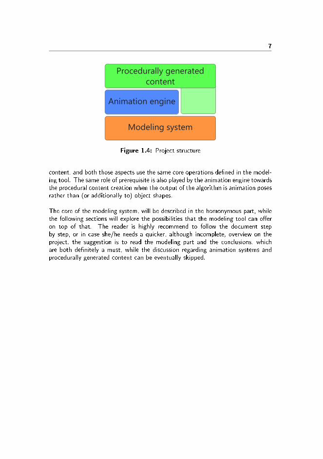
The modeling tool isn't only a good start point for the project but it is also afundamental prerequisite for the animation system and the procedurally generated

7

Procedurally generated

content

Animation engine

Modeling system

Figure 1.4: Project structure

content, and both those aspects use the same core operations de�ned in the model-ing tool. The same role of prerequisite is also played by the animation engine towardsthe procedural content creation when the output of the algorithm is animation posesrather than (or additionally to) object shapes.

The core of the modeling system, will be described in the homonymous part, whilethe following sections will explore the possibilities that the modeling tool can o�eron top of that. The reader is highly recommend to follow the document stepby step, or in case she/he needs a quicker, although incomplete, overview on theproject, the suggestion is to read the modeling part and the conclusions, whichare both de�nitely a must, while the discussion regarding animation systems andprocedurally generated content can be eventually skipped.

8

Part I

Modeling

Chapter 2

A new modeling system

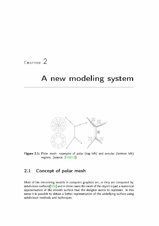
Figure 2.1: Polar mesh: examples of polar (top left) and annular (bottom left)regions. (source: [JAB12])

2.1 Concept of polar mesh

Most of the interesting models in computer graphics are, or they are composed by,subdivision surfaces[Wik] and in these cases the mesh of the object is just a numericalapproximation of the smooth surface that the designer wants to represent. In thissense it is possible to obtain a better representation of the underlying surface usingsubdivision methods and techniques.

12 A new modeling system

As presented by Thomas J. Cashman, over the past 15 years di�erent subdivisionschema have been developed, and nowadays they are a fundamental component ofevery modeling system. The standard de facto in this �eld is Catmull-Clark, the�very �rst subdivision schema for surfaces� [Cas12] that inspired several others, allbased on recursion of simple rules.

An easy way to de�ne subdivision surfaces is using �a sequence of nested spline ringsconverging to an extraordinary point� [KP07a], and in this case Catmull-Clark (andmost of the other methods) poorly performs, especially when the valence is high.

Kar£iauskas and Peter, instead, proposed an alternative layout where the valency canbe progressively adjusted in such a way that if n is the valency of the extraordinarypoint, then each ring is a sequence of n segments smoothly interconnected. Meshesthat shows this layout are called polar regions and they completely avoids the typicalcorners yield by the Catmull-Clark subdivision schema. As an extension, it is alsopossible to de�ne annular regions, where the extraordinary point has been removedtogether with the triangle fan that it supports.

A mesh composed by an interconnected set of polar and annular regions is calledpolar mesh [JAB12]and it supports and has a closure under the polar subdivisionschema.

2.2 SQM: Skeleton to Quad Mesh

Figure 2.2: ZBrush: usage of ZSpheres to de�ne the model's structure (left) beforecreating the polygonal mesh (right). Source: http://pixologic.com/

2.2 SQM: Skeleton to Quad Mesh 13

Skeletons are the de facto standard for most of the animations that are daily im-plemented in the 3D industry, however in the typical production pipeline the meshis �rstly created and later skinned to match its skeleton. It is important to noticethat, in this case, the CGI artist doesn't exploit the shape information that he canget from an easy to create skeleton: not only the high poly mesh is created directlyfrom scratch but later it has to be manually skinned to match its skeleton, so thedesigner has to deal twice with a complex mesh object rather than exploit a simpleskeleton structure.

In their work J. A. Bærentzen, M. K. Misztal and K. Welnicka �ipped all of this:they developed an algorithm to procedurally generate a polar mesh based on a givenskeleton (SQM: Skeleton to Quad Mesh[JAB12]). A similar approach is also usedin Z-Brush, the well known modeling software, and it requires that the CGI Artistdesigns a skeleton for the object before the mesh generation.

In SQM the CGI artist models the skeleton, that is considerably simpler than a fullhigh poly object, then he just needs to procedurally generate the �nal mesh. In�gure 2.3 it is shown an example.

This method surely requires CGI artists with good abstraction skills, as it isn't alwayseasy to recognize the right skeleton for a desired polygonal mesh, but it is incrediblyfaster than any traditional sculpturing tool.

Figure 2.3: SQM: example from Bærentzen's paper [JAB12]

14 A new modeling system

2.3 This project as an evolution of SQM

In his thesis [Don12], Michael Mc Donnell proved that SQM is a fairly good toolto model rough organic objects, but it su�ers from severe limitations when theobject that needs to be shaped is inorganic or it hasn't a clear structure. His initialassumption was that these limitations can be overcome with a richer set of skeletonnodes. This wasn't only supported by Leblanc's work [LLP11], but somehow it alsomakes sense: the skeleton de�nes the branching structure of the entire objects butit lacks of all the skin details. Imagine to �nd the bones of an alien, not the skinjust the skeleton; is it really possible to infer its silhouette? Not really. In the sameway SQM can guess the skin of the skeleton that has been modeled, but additionalinformation is needed in order to correctly infer the right mesh.

It turned out that a richer set of nodes isn't enough to substantially expand theexpressiveness of the SQM method, that remains strongly limited in its original�eld.

From this point of view, this thesis represents an evolution of the SQM method,but it does it from di�erent considerations, those leads to a completely di�erentmodeling system.

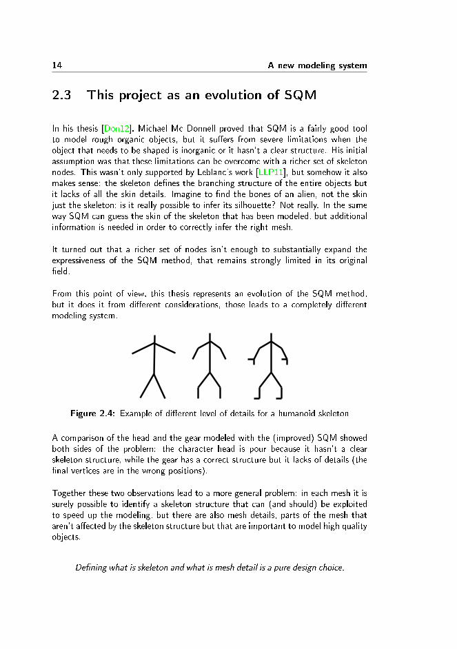
Figure 2.4: Example of di�erent level of details for a humanoid skeleton

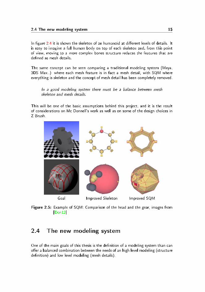
A comparison of the head and the gear modeled with the (improved) SQM showedboth sides of the problem: the character head is pour because it hasn't a clearskeleton structure, while the gear has a correct structure but it lacks of details (the�nal vertices are in the wrong positions).

Together these two observations lead to a more general problem: in each mesh it issurely possible to identify a skeleton structure that can (and should) be exploitedto speed up the modeling, but there are also mesh details, parts of the mesh thataren't a�ected by the skeleton structure but that are important to model high qualityobjects.

De�ning what is skeleton and what is mesh detail is a pure design choice.

2.4 The new modeling system 15

In �gure 2.4 it is shown the skeleton of an humanoid at di�erent levels of details. Itis easy to imagine a full human body on top of each skeleton and, from this pointof view, moving to a more complex bones structure reduces the features that arede�ned as mesh details.

The same concept can be seen comparing a traditional modeling system (Maya,3DS Max..) where each mesh feature is in fact a mesh detail, with SQM whereeverything is skeleton and the concept of mesh detail has been completely removed.

In a good modeling system there must be a balance between meshskeleton and mesh details.

This will be one of the basic assumptions behind this project, and it is the resultof considerations on Mc Donnell's work as well as on some of the design choices inZ-Brush.

Goal Improved Skeleton Improved SQM

Figure 2.5: Example of SQM: Comparison of the head and the gear, images from[Don12]

2.4 The new modeling system

One of the main goals of this thesis is the de�nition of a modeling system than cano�er a balanced combination between the needs of an high level modeling (structurede�nition) and low level modeling (mesh details).

16 A new modeling system

Two di�erent set of operations will be used to make the de�nition of the meshstructure (and consequently its skeleton) easy and fast, as well as to model meshdetails with precise vertices placement:

The High level modeling: a set of operations that interact with the polar struc-ture of the model:

� Add/Remove Re�nement: increase or decrease the valency of a pole

� Add/Remove feature: create or remove a branch on the speci�ed po-sition.

� Merge/Split feature(s): merge two polar regions on a single annularregion. In the inverse operation an annular/polar region is split in twoseparate polar regions.

Low level modeling: the mesh details instead can be fully de�ned with the 3 mosttraditional mesh operations. Please note how none of the following tools cana�ect the mesh structure in any way:

� Move: translate the selected group of vertices

� Scale: increase or decrease the relative distance of a group of vertices

� Rotate: spin the selected group of vertices around its relative center

The bene�ts of this approach will be proved developing a prototype that will strictlysupport only this new modeling paradigm, where the mesh operations will be closedtowards the polar/annular property (each operation will be applied to a polar meshand it will output a polar mesh) and the mesh skeleton will be inferred run-timedirectly from the mesh vertices. In order to test the real expressiveness of thisapproach no additional post-processing will be supported.

2.5 Consideration on mesh topology

2.5.1 Triangles vs Quad dominant meshes

Although the rendering systems historically support mesh based on arbitrary (con-vex) polygons, today the entire modeling world processes only quad or trianglesbased meshes. The main reason for this evolution is the huge performance bene�tsleaded both by the limited number of vertices per primitive and the hardware paral-lelization that characterizes modern GPUs; but although both the recent GPUs and

17

the rendering engines are designed, implemented and optimized for triangle basedmeshes, designer and CGI Artists often prefer quads.

Quad dominant meshes have two big bene�ts [Dil] compared to triangles basedmeshes:

Subdivision methods: there are subdivision methods that work on triangles as well(√3 Subdivision by Kobbelt [Kob00] for example), but quad based subdivision

methods give, in general, a better control to the designer regarding the desiredlevel of detail and they yield more balanced meshes.

Edge loops: another interesting aspect is the de�nition and preservation of edgeloops, set of connected edges that de�ne close rings. It is easy to prove thatgeneral triangle meshes don't easily yield edge loops, simply due to their oddnumber of vertices per primitive, but edge loops are an important feature toavoid artifacts on animations that involve blending and folding.

Figure 2.6: Polar Mesh: edge loops highlithed in red.

2.5.2 Polar meshes from a topology prospective

Polar meshes are surely an interesting case of quad dominant meshes and theyfully preserve edge loop structure: as previously de�ned a polar mesh is a smoothlyinterconnected set of polar and annular regions, each of them de�ned as a sequenceof spline rings. It is trivial to see that each spline ring is in fact an edges loop.

Polar meshes naturally supports the polar subdivision schema [KP07b], a subdivisionmethods that changes the valency of the polar/annular region without compromisingthe loops of edges.

18

Chapter 3

Polar Meshes

Polar meshes can be more formally de�ned with few de�nitions:

Annular region If Q = (q1, q2..qn) is a tuple of quads, each of them de�ned byfour edges qi = (hi1, hi2, hi3, hi4), Q is called an annular region if ∀qi ∈ Q hi1 =h(i−1)3 ∧ hi3 = h(i+1)1. In this case the tuples L1 = (h12, h22, ..hn2) and L2 =(h14, h24, ..hn4) are nested spline rings and they are called loops of the annularregion.

Pole and pole region A pole is a vertex p center of the triangle fan T =(t1, t2..tn), marked as a �pole�. If each triangle is de�ned by ∀ti ∈ T ti =(p, hi, hmodn(i+1)), than L = (h0, ..hn) is called loop of the pole. T , the trian-gle fan itself is called pole region.

Loop A loop is a tuple of edges L = (h0, ..hn), where each edge hi ∈ L is de�nedby two vertices hi = (vi, vmodn(i+1)).

For each loop in the mesh, there are at least 2 elements that share the loop, whichare either annular or polar regions;

20 Polar Meshes

For each loop edge in the mesh there are exactly 2 elements that share the loop,which are either annular or polar regions;

Backbone A backbone is a connected path of non-loop edges either between twopoles or that loop itself:

� if the backbone, de�ned as the tuple of edges B = (h0, ..hn), is a pathbetween the poles p1, p2, then each edge is de�ned by two vertices ∀hi ∈B \ {h0, hn} hi = (vi, vi+1), h0 = (p1, v2) and hn = (hn−1, p2).

� if the backbone, de�ned as the tuple of edges B = (h0, ..hn), is a closed path,then each edge is de�ned by two vertices ∀hi ∈ B hi = (vi, vmodn(i+1)).

In both cases none of the internal edges can be part of a loop: ∀hi ∈ B ¬∃L inthe mesh |hi ∈ L (design constrain).

Figure 3.1: Polar mesh: example

3.1 Notation

In order to keep a precise but concise description, for the following sections a math-ematical notation will be used to describe polar mesh components and some basicoperations that a�ect them:

3.1 Notation 21

3.1.1 Mesh elements

V set of vertices of the mesh

P ⊆ V set of poles of the mesh

H set of halfedges of the mesh

F set of faces of the mesh

3.1.2 Properties of mesh elements

3.1.2.1 Vertices

v = vert(h) vertex v ∈ V pointed by the halfedge h ∈ H

Vx = vert(Hx) Vx = {vert(h)|h ∈ Hx ⊆ H}Hx = out(v) set of halfedges Hx outgoing from the vertex v

Hx = out(Vx) Hx = {out(v)|v ∈ Vx ⊆ V }p = pos(v) position of the vertex v in global coordinates

3.1.2.2 Faces

f = face(h) face f ∈ F associated with the half edge h ∈ H.

Fx = face(Hx) Fx = {face(h)|h ∈ Hx ⊆ H}Hx =

halfedges(f)

Hx = {h ∈ H|f = face(h)}, in other words Hx is the set of

halfedges that de�nes the face f

Hx =

halfedges(Fx)

Hx = {halfedges(f)|f ∈ Fx ⊆ F}

3.1.3 Basic mesh navigation

h2 = opp(h1) if h1 ∈ H exists between v1 ∈ V and v2 ∈ V , such as

v1 = vert(h1), then h2 ∈ H exists between v1 and v2 and

v2 = vert(h2)

h2 = next(h1) h2 immediately follows h1in the de�nition of f = face(h1), with

h1 ∈ H and h2 ∈ halfedges(face(h1))

h2 = prev(h1) if h1 = next(h2), with h1 ∈ H and h2 ∈ halfedges(face(h1)). In

other words h2 immediately precedes h1in the de�nition of

f = face(h1)

22 Polar Meshes

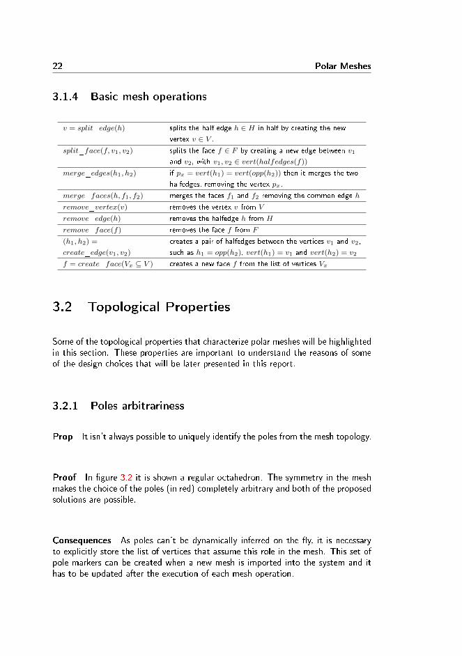
3.1.4 Basic mesh operations

v = split_edge(h) splits the half edge h ∈ H in half by creating the new

vertex v ∈ V .

split_face(f, v1, v2) splits the face f ∈ F by creating a new edge between v1

and v2, with v1, v2 ∈ vert(halfedges(f))

merge_edges(h1, h2) if px = vert(h1) = vert(opp(h2)) then it merges the two

halfedges, removing the vertex px.

merge_faces(h, f1, f2) merges the faces f1 and f2 removing the common edge h

remove_vertex(v) removes the vertex v from V

remove_edge(h) removes the halfedge h from H

remove_face(f) removes the face f from F

(h1, h2) =

create_edge(v1, v2)

creates a pair of halfedges between the vertices v1 and v2,

such as h1 = opp(h2), vert(h1) = v1 and vert(h2) = v2

f = create_face(Vx ⊆ V ) creates a new face f from the list of vertices Vx

3.2 Topological Properties

Some of the topological properties that characterize polar meshes will be highlightedin this section. These properties are important to understand the reasons of someof the design choices that will be later presented in this report.

3.2.1 Poles arbitrariness

Prop It isn't always possible to uniquely identify the poles from the mesh topology.

Proof In �gure 3.2 it is shown a regular octahedron. The symmetry in the meshmakes the choice of the poles (in red) completely arbitrary and both of the proposedsolutions are possible.

Consequences As poles can't be dynamically inferred on the �y, it is necessaryto explicitly store the list of vertices that assume this role in the mesh. This set ofpole markers can be created when a new mesh is imported into the system and ithas to be updated after the execution of each mesh operation.

3.2 Topological Properties 23

Figure 3.2: Poles arbitrariness: visual proof

3.2.2 Loops arbitrariness

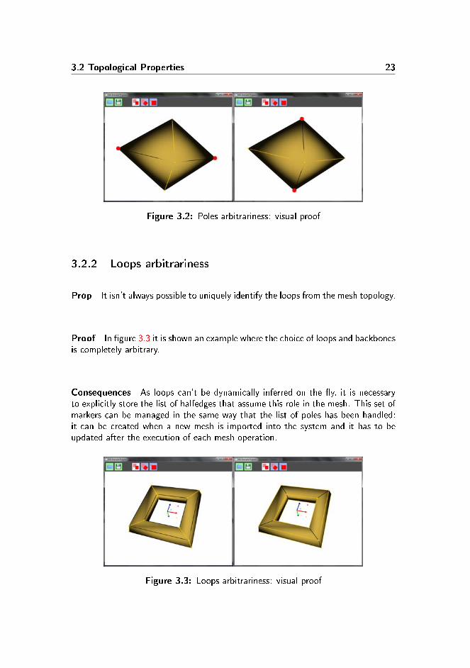
Prop It isn't always possible to uniquely identify the loops from the mesh topology.

Proof In �gure 3.3 it is shown an example where the choice of loops and backbonesis completely arbitrary.

Consequences As loops can't be dynamically inferred on the �y, it is necessaryto explicitly store the list of halfedges that assume this role in the mesh. This set ofmarkers can be managed in the same way that the list of poles has been handled:it can be created when a new mesh is imported into the system and it has to beupdated after the execution of each mesh operation.

Figure 3.3: Loops arbitrariness: visual proof

24 Polar Meshes

3.2.3 Loop and backbone connectivity

Prop

� If h is a loop edge, then next(h) is a backbone edge.

� If k is a backbone edge and vert(k) isn't a pole, then next(k) is a loop edge.

Proof To demonstrate both sentences, lets analyze annular and polar regions sep-arately:

� In annular regions each quad is by de�nition a sequence of backbone-loop-backbone-loop edges, therefore both propositions are trivially true.

� In polar regions instead each triangle is de�ned by a loop edge followed by 2backbone edges. As the pole is always between these last two, it is easy tosee that both statements are true also in polar regions.

3.3 Iterators

A key prerequisite of all the operations that have been implemented is their abilityto navigate the mesh. Some halfedge iterators has been built for this purpose:

Loop iterator: given an half edge, it walks along the entire loop or backbone wherethe half edge lies.

Parallel iterator: given an half edge, it iterates through all the half edges that areparallel to the initial one.

Fan iterator: given a pole, it iterates through all the halfedges outgoing from thepole

3.3.1 Loop iterator

Input h0 ∈ HOutput O = {h0} ∪ {next(opp(next(h)))|h ∈ O ∧ vert(h) /∈

P} ∪ {prev(opp(prev(h)))|h ∈ O ∧ vert(opp(h)) /∈ P}Function O = Loop(h0)

3.4 Features 25

3.3.2 Parallel iterator

Input h0 ∈ HOutput B = Loop(next(h0)) if vert(h0) /∈ P

B = Loop(prev(h0)) otherwise.O = {next(h)|h ∈ B ∧ vert(h) /∈ P}

Function O = Parallel(h0)

3.3.3 Fan iterator

Input p ∈ POutput O = {h|h ∈ H ∧ vert(opp(h)) = p}Function O = Fan(p)

3.4 Features

3.4.1 De�nitions

Nesting Loop A nesting Loop is a Loop of the mesh that supports a breach inthe mesh skeleton. More formally a nesting loop is a loop L = (h0, ..hn) where∃hi ∈ L|valency(hi) > 4 ∧ vert(hi) isn't pole.

Skeleton segment A skeleton segment is what most of 3D modeling systems callbone and it is an abstract representation of an annular or polar region:

Annular region: de�ned by the loops L0 and L1 implicitly de�nes the skeleton seg-ment S between the points P0 = 1

|L0|∑

pos(vert(L0)) and P1 =1|L1|

∑pos(vert(L1)).

Polar region: de�ned by the pole P and the loop L implicitly de�nes the skeletonsegment S between the points P and P1 = 1

|L|∑

pos(vert(L)).

Feature A feature is a group of polar and annular regions that implicitly de�nes achain of consecutive and connected skeleton segments between 2 nesting loops, or2 poles or 1 nesting loop and 1 pole. These elements are called boundaries of thefeature.

26

3.4.2 Child features

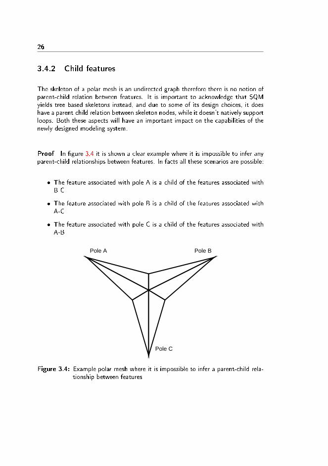
The skeleton of a polar mesh is an undirected graph therefore there is no notion ofparent-child relation between features. It is important to acknowledge that SQMyields tree based skeletons instead, and due to some of its design choices, it doeshave a parent-child relation between skeleton nodes, while it doesn't natively supportloops. Both these aspects will have an important impact on the capabilities of thenewly designed modeling system.

Proof In �gure 3.4 it is shown a clear example where it is impossible to infer anyparent-child relationships between features. In facts all these scenarios are possible:

� The feature associated with pole A is a child of the features associated withB-C

� The feature associated with pole B is a child of the features associated withA-C

� The feature associated with pole C is a child of the features associated withA-B

Pole A Pole B

Pole C

Figure 3.4: Example polar mesh where it is impossible to infer a parent-child rela-tionship between features

Chapter 4

Core Operations

In this chapter it will be presented the 7 polar mesh operations that have beendesigned, implemented and tested. These operations represent the core of the highlevel modeling system and they concretely increase the abstraction level of the toolthat has been developed.

4.1 Add re�nement

Add a loop or a backbone at the speci�ed point. Conceptually:

� when a loop is added, it generates a new annular region from an existing polaror annular region

� when a backbone is added, it increase the valency of the interested regions.

4.1.1 Speci�cation

1 vo i d addRef inement ( ha l fEdge h0 )

28 Core Operations

h0 is one of the half edges those will be splitted during the operation. In generalH0 = Parallel(h0 ∈ H) are all and only the a�ected half edges.

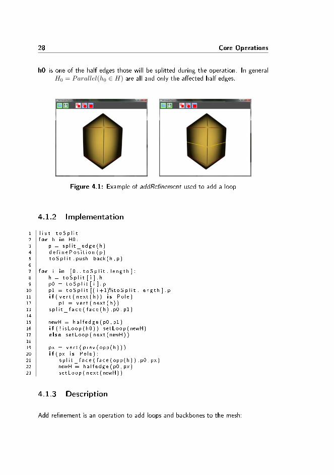
Figure 4.1: Example of addRe�nement used to add a loop

4.1.2 Implementation

1 l i s t t o S p l i t2 f o r h i n H0 :3 p = sp l i t_edg e ( h )4 d e f i n e P o s i t i o n ( p )5 t o S p l i t . push_back (h , p )6

7 f o r i i n [ 0 . . t o S p l i t . l e n g t h ] :8 h = t o S p l i t [ i ] . h9 p0 = t o S p l i t [ i ] . p

10 p1 = t o S p l i t [ ( i +1)%t o S p l i t . l e n g t h ] . p11 i f ( v e r t ( nex t ( h ) ) i s Pole ) :12 p1 = v e r t ( nex t ( h ) )13 s p l i t_ f a c e ( f a c e ( h ) , p0 , p1 )14

15 newH = ha l f e d g e ( p0 , p1 )16 i f ( ! i sLoop ( h0 ) ) se tLoop (newH)17 e l s e se tLoop ( next (newH) )18

19 px = v e r t ( p r ev ( opp ( h ) ) )20 i f ( px i s Pole ) :21 s p l i t_ f a c e ( f a c e ( opp ( h ) ) , p0 , px )22 newH = ha l f e d g e ( p0 , px )23 se tLoop ( next (newH) )

4.1.3 Description

Add re�nement is an operation to add loops and backbones to the mesh:

4.2 Remove re�nement 29

� to add a loop, addRe�nement needs to be applied to one of the backboneedges that is going to be splitted with the new loop.

� to add a backbone, addRe�nement needs to be applied to one of the loopedges that is going to be splitted with the new backbone.

The algorithm operates in 3 steps:

1. it collects all the edges that are parallel to the given parameter, until it closes aloop or it will reach the extreme poles (standard usage of the parallel iterator).

2. it splits the collected edges with new vertices

3. it splits the faces associated with the collected edges, generating the newre�nement and it marks the newly created edges as loops and backbones.

4.1.4 Limitations

AddRe�nement can be applied to every edge of the mesh without any speci�climitation.

4.2 Remove re�nement

Remove a loop or a backbone from the mesh. Conceptually:

� when a loop is removed, it merges an annular region into a polar region orinto another annular region

� when a backbone is removed, it reduced the valency of the interested regions

4.2.1 Speci�cation

1 vo i d removeRef inement ( ha l fEdge h0 )

h0 is one of the half edges that are part of the re�nement that needs to be removed.In general all edges in H0 = Loop(h0 ∈ H) will be removed at the end of theoperation, which can be applied if and only if ∀h ∈ Loop(h0) Loop(h) =

30 Core Operations

Loop(h0), or in other words if and only if the selected half edge isn't part ofa loop where a feature is nested.

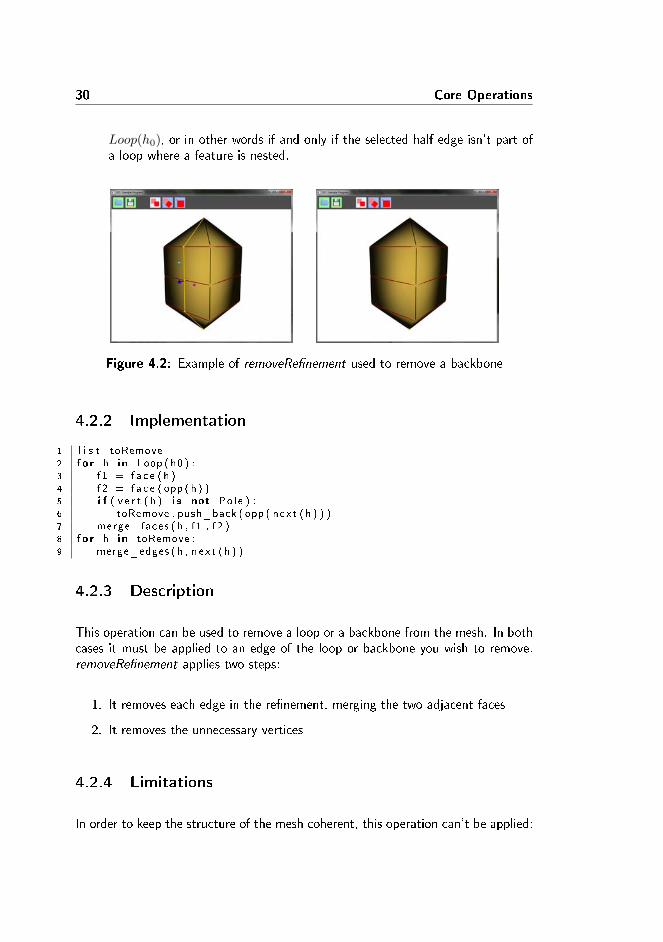
Figure 4.2: Example of removeRe�nement used to remove a backbone

4.2.2 Implementation

1 l i s t toRemove2 f o r h i n Loop ( h0 ) :3 f 1 = f a c e ( h )4 f 2 = f a c e ( opp ( h ) )5 i f ( v e r t ( h ) i s not Pole ) :6 toRemove . push_back ( opp ( next ( h ) ) )7 merge_faces (h , f1 , f 2 )8 f o r h i n toRemove :9 merge_edges (h , nex t ( h ) )

4.2.3 Description

This operation can be used to remove a loop or a backbone from the mesh. In bothcases it must be applied to an edge of the loop or backbone you wish to remove.removeRe�nement applies two steps:

1. It removes each edge in the re�nement, merging the two adjacent faces

2. It removes the unnecessary vertices

4.2.4 Limitations

In order to keep the structure of the mesh coherent, this operation can't be applied:

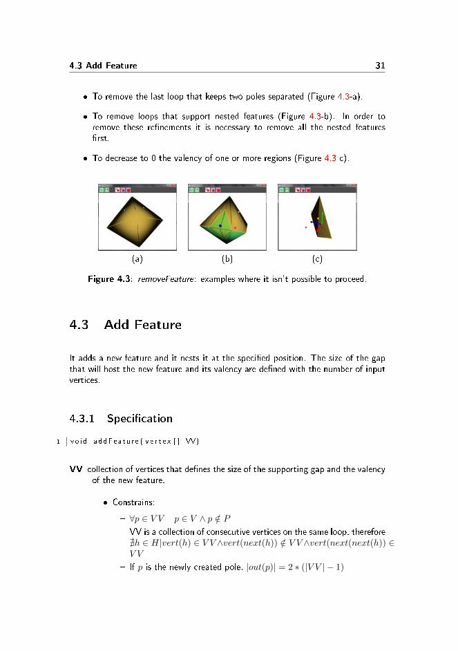
4.3 Add Feature 31

� To remove the last loop that keeps two poles separated (Figure 4.3-a).

� To remove loops that support nested features (Figure 4.3-b). In order toremove these re�nements it is necessary to remove all the nested features�rst.

� To decrease to 0 the valency of one or more regions (Figure 4.3-c).

(a) (b) (c)

Figure 4.3: removeFeature: examples where it isn't possible to proceed.

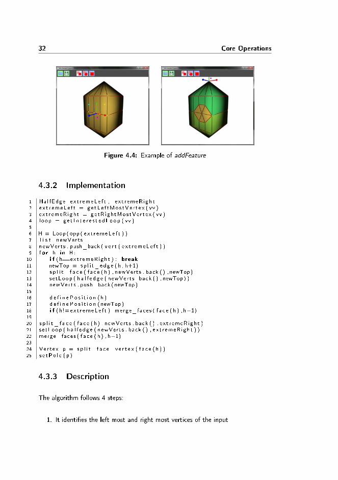
4.3 Add Feature

It adds a new feature and it nests it at the speci�ed position. The size of the gapthat will host the new feature and its valency are de�ned with the number of inputvertices.

4.3.1 Speci�cation

1 vo i d addFeature ( v e r t e x [ ] VV)

VV collection of vertices that de�nes the size of the supporting gap and the valencyof the new feature.

� Constrains:

� ∀p ∈ V V p ∈ V ∧ p /∈ P

� VV is a collection of consecutive vertices on the same loop, therefore@h ∈ H|vert(h) ∈ V V ∧vert(next(h)) /∈ V V ∧vert(next(next(h)) ∈V V

� If p is the newly created pole, |out(p)| = 2 ∗ (|V V | − 1)

32 Core Operations

Figure 4.4: Example of addFeature

4.3.2 Implementation

1 Hal fEdge ex t r emeLe f t , e x t r emeR igh t2 e x t r emeLe f t = ge tLe f tMos tVe r t e x ( vv )3 ex t r emeR ight = getR ightMos tVe r t ex ( vv )4 l oop = g e t I n t e r e s t e d L o op ( vv )5

6 H = Loop ( opp ( e x t r emeLe f t ) )7 l i s t newVerts8 newVerts . push_back ( v e r t ( e x t r emeLe f t ) )9 f o r h i n H:

10 i f ( h==ext r emeR ight ) : break11 newTop = sp l i t_edg e (h , h+1)12 s p l i t_ f a c e ( f a c e ( h ) , newVerts . back ( ) , newTop )13 se tLoop ( h a l f e d g e ( newVerts . back ( ) , newTop ) )14 newVerts . push_back (newTop )15

16 d e f i n e P o s i t i o n ( h )17 d e f i n e P o s i t i o n ( newTop )18 i f ( h!= ex t r emeLe f t ) merge_faces ( f a c e ( h ) , h−1)19

20 s p l i t_ f a c e ( f a c e ( h ) , newVerts . back ( ) , ex t r emeR ight )21 se tLoop ( h a l f e d g e ( newVerts . back ( ) , ex t r emeR igh t ) )22 merge_faces ( f a c e ( h ) , h−1)23

24 Ver tex p = sp l i t_ f a c e_v e r t e x ( f a c e ( h ) )25 s e tPo l e ( p )

4.3.3 Description

The algorithm follows 4 steps:

1. It identi�es the left most and right most vertices of the input

4.4 Select Feature 33

2. It iterates over the selected vertices left to right, splitting the top faces in orderto generate the upper side of the loop gap. It reuse the existing loop to de�nethe lower side and it sets the newly generated edges as loop components.

3. It merges the inner faces in a single big polygon

4. It creates the �nal triangle fan splitting the big polygon with a vertex

4.3.4 Limitations

� Features must be nested on skeleton nodes, therefore it isn't possible to de�nefeatures along backbones, only on loops (Figure 4.5-a).

� It is possible to nest several features on the same skeleton node, therefore itis possible to de�ne multiple features on the same loop (Figure 4.5-b).

� It is possible to de�ne features on loop edges that are the boundary of anexisting nested feature (Figure 4.5-c).

� It isn't possible to de�ne features only partially overlapped with other featuresor, in other words, if a loop supports nested features, then it must supportthe entire features' gap (Figure 4.5-d).

(a) (b) (c) (d)

Figure 4.5: addFeature: examples.

4.4 Select Feature

Identify and select all the components of the feature associated with the given face.

4.4.1 Speci�cation

1 se t<face s > s e l e c t F e a t u r e ( f a c e f )

34 Core Operations

f face of the mesh

return the set of faces that are part of the same feature of f

4.4.2 Implementation

1 r e t = new set<face s >()2 b = getBackboneEdge ( f )3 B = Loop ( b )4 f e a tu r eFound=f a l s e5 f o r backbone i n B:6 i f ( f ea tu r eFound ) : break7 i f ( i s P o l e ( v e r t ( backbone ) ) ) :8 fanLoop = Fan ( v e r t ( backbone ) ) :9 f o r l i n fanLoop :

10 r e t . push_back ( f a c e ( l ) )11 break12 l oop = Loop ( next ( backbone ) )13 f o r l i n l oop :14 r e t . push_back ( f a c e ( l ) )15 i f ( v a l e n c y ( v e r t ( l ) )>4) :16 f e a tu r eFound=t r u e17

18 i f ( f ea tu r eFound ) :19 B = Loop ( opp ( b ) )20 f o r backbone i n B:21 i f ( f ea tu r eFound ) : break22 i f ( i s P o l e ( v e r t ( backbone ) ) ) :23 fanLoop = Fan ( v e r t ( backbone ) ) :24 f o r l i n fanLoop :25 r e t . push_back ( f a c e ( l ) )26 break27 l oop = Loop ( next ( backbone ) )28 f o r l i n l oop :29 r e t . push_back ( f a c e ( l ) )30 i f ( v a l e n c y ( v e r t ( l ) )>4) :31 f e a tu r eFound=t r u e32

33 re tu rn r e t

4.4.3 Description

First of all, the algorithm identi�es a backbone edge of the input face, then it movesforward and backwards along that backbone adding each loop to the result set. Theprocess stop when one of the following conditions is met:

� The backbone loops and the algorithm is at the original start point.

4.5 Remove Feature 35

� A pole is reached and the polar region is added to the result set.

� A vertex with higher valency is detected, unique sign of the presence of nestedfeatures.

4.5 Remove Feature

Remove the feature associated with the given face.

4.5.1 Speci�cation

1 vo i d removeFeature ( f a c e f )

f face associated to the feature to remove.

� Constrains:

� In the loop that represent the boundary of the feature there mustbe exactly two vertices with valency higher than 4 (split vertices)

� Along the boundary loop, the split vertices are connected with twodi�erent paths. These paths must have the same number of internalvertices.

Figure 4.6: Example of removeFeature

4.5.2 Implementation

36 Core Operations

1 po l e = ge tFea t u r ePo l e ( f )2 B = Loop ( out ( po l e ) )3 // 1 − S t r u c t u r a l check4 f e a tu r eFound = f a l s e5 f o r backbone i n B:6 i f ( f ea tu r eFound ) : break7 l oop = Loop ( next ( backbone ) )8 f o r l i n l oop :9 i f i s S p l i t ( l ) :

10 i f ( ! i s G o o dSp l i t P o i n t ( l ) ) re tu rn11 s p l i t E d g e = l12 stopLoop = next ( backbone )13 f e a tu r eFound=t r u e14 break15

16 // 2 − Remove i n t e r n a l l o op s17 f e a tu r eFound=f a l s e18 whi le ( ! f ea tu r eFound ) :19 Hal fEdgeID b = out ( po l e )20 Hal fEdgeID h = next ( b )21 L = Loop ( h )22 f o r l i i n L :23 i f ( l i . i s S p l i t ( ) ) : f ea tu r eFound=t r u e24 i f ( ! f ea tu r eFound ) removeLoops ( h )25

26 // 3 − Prepa re edge l i s t s27 L1 = Loop ( s p l i t E d g e )28 L2 = Loop ( s p l i t E d g e )29 l i s t faceTop , faceBottom , edgeTop , edgeBottom30 i 1=131 i 2=032 do :33 i 2=( i 2 +1)%L2 . l e n g t h34 i 1 = ( i1 −1)%L1 . l e n g t h35 l 1=L1 [ i 1 ]36 l 2=L2 [ i 2 ]37 faceTop . push_back ( f a c e ( ck . opp ( l 1 ) ) )38 faceBottom . push_back ( f a c e ( opp ( l 2 ) ) )39 edgesTop . push_back ( l 1 )40 edgesBottom . push_back ( l 2 )41 pos ( v e r t ( l 2 ) ) = ( pos ( v e r t ( l 2 ) )+pos ( v e r t ( opp ( l 1 ) ) ) ) /2 .0 f42 whi le ( v e r t ( l 2 ) != v e r t ( opp ( l 1 ) ) )43

44 // 4 − Remove t r i a n g l e fan45 F = Fa n I t e r a t o r ( po l e )46 f o r f i i n F :47 remove_face ( f a c e ( f i ) )48 remove_edge ( opp ( f i ) )49 remove_edge ( f i )50

51 remove_vertex ( po l e )52

53 // 5 − F i x S t r u c t u r e54 eTop = edgesTop . beg in ( )55 eBottom = edgesBottom . beg in ( )

4.5 Remove Feature 37

56 fTop = faceTop . beg in ( )57 fBottom = faceBottom . beg in ( )58 whi le ( eTop!=edgesTop . end ( ) ) :59 s e t_ve r t ( opp ( eTop ) , v e r t ( eBottom ) )60 s e t_ve r t ( opp ( next ( opp ( eTop ) ) ) , v e r t ( eBottom ) )61

62 s e t_ve r t ( eTop , v e r t ( opp ( eBottom ) ) )63 s e t_ve r t ( p r ev ( opp ( eTop ) ) , v e r t ( opp ( eBottom ) ) )64

65 s e t_face ( eBottom , f a c e ( opp ( eTop ) ) )66 connect_next_and_prev ( p r ev ( opp ( eTop ) ) , eBottom , , nex t ( opp ( eTop ) ) )67

68 s e t_ l a s t ( fTop , eBottom )69 set_out ( v e r t ( eBottom ) , opp ( eBottom ) )70 set_out ( v e r t ( opp ( eBottom ) ) , eBottom )71

72 i f ( v e r t ( eTop ) != v e r t ( opp ( eBottom ) ) )73 remove_vertex ( ck . v e r t ( eTop ) )74

75 remove_edge ( opp ( eTop ) )76 remove_edge ( eTop )77

78 ++eTop79 ++eBottom80 ++fTop81 ++fBottom

4.5.3 Description

To remove an existing feature several steps are necessary:

1. Check the structure to identify the split vertices (valency higher than 4). Ifmore than 2 split vertices are detected or if they are placed in inconvenientpositions, the operation is aborted.

2. Remove all internal loops to reduce the feature to a triangle fan

3. Adjust vertices position

4. Remove the triangle fan

5. Close the gap, paring and merging top and bottom faces.

4.5.4 Limitations

A �rst important limitation is actually related to the current prototype implementa-tion: it is possible to remove features only if they are bounded between a loop and

38 Core Operations

a pole. Features bounded by two loops can't be removed straight away but theyneed to be �rstly splitted and then removed with a distinct operation.

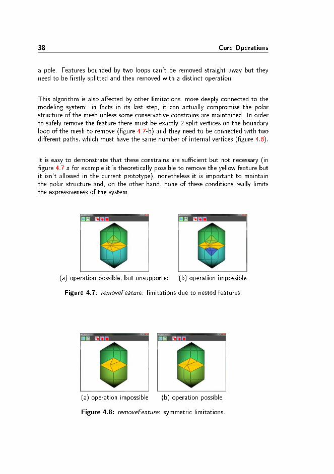
This algorithm is also a�ected by other limitations, more deeply connected to themodeling system: in facts in its last step, it can actually compromise the polarstructure of the mesh unless some conservative constrains are maintained. In orderto safely remove the feature there must be exactly 2 split vertices on the boundaryloop of the mesh to remove (�gure 4.7-b) and they need to be connected with twodi�erent paths, which must have the same number of internal vertices (�gure 4.8).

It is easy to demonstrate that these constrains are su�cient but not necessary (in�gure 4.7-a for example it is theoretically possible to remove the yellow feature butit isn't allowed in the current prototype), nonetheless it is important to maintainthe polar structure and, on the other hand, none of these conditions really limitsthe expressiveness of the system.

(a) operation possible, but unsupported (b) operation impossible

Figure 4.7: removeFeature: limitations due to nested features.

(a) operation impossible (b) operation possible

Figure 4.8: removeFeature: symmetric limitations.

4.6 Merge Features 39

4.6 Merge Features

Merge two features, bridging the poles

4.6.1 Speci�cation

1 vo i d mergeFeature ( v e r t e x p1 , v e r t e x p2 )

p1 pole associated with the �rst feature

� Constrains: p1 ∈ P

p2 pole associated with the second feature

� Constrains: p2 ∈ P , valency(p2) = valency(p1)

Figure 4.9: Example of mergeFeature

4.6.2 Implementation

1 f an1 = Fan ( p1 )2 f an2 = Fan ( p2 )3

4 // 1 − f i n d i ndex o f v e r t e c i s a t min d i s t a n c e5 ( i1 , i 2 )=ve r t e c i s_min_d i s t anc e ( fan1 , fan2 )6

7 // 2 − remove t r i a n g l e f a n s8 f o r i i n [ 0 . . f an1 . l e n g t h ] :9 remove_face ( f a c e ( fan1 [ i ] ) )

10 remove_face ( f a c e ( fan2 [ i ] ) )11 a r r a y L i s t edges

40 Core Operations

12

13 // 3 − b r i d g e l o op s14 f o r i i n [ 0 . . f an1 . l e n g t h ] :15 p a i r ( h1 , h2 )=create_edge ( v e r t ( fan1 [ i ] ) , v e r t ( fan2 [ i ] ) )16 edges . push_back ( p a i r ( h1 , h2 ) )17 f o r i i n [ 0 . . f an1 . l e n g t h ] :18 hh0 = fan1 [ i ]19 hh1 = edges [ i ] . h120 hh2 = opp ( fan2 [ i ] )21 hh3 = edges [ ( i −1)%fan1 . l e n g t h ] . h222 c r e a t e_ fac e ( hh0 , hh1 , hh2 , hh3 )

4.6.3 Description

In order to merge two features, identi�ed by the 2 given poles, the following stepsare necessary:

1. Find a match between the vertices of the two base loops. In the currentimplementation the risk of a twist e�ects has been minimized using the closestvertices to initialize the pairing procedure.

2. pairing the closest vertices together.

3. Remove the two triangles fans

4. Bridge the loops, generating new halfedges and new faces between the matchedvertices.

4.6.4 Limitations

mergeFeature can be applied to any pole pairs, as long as their valencies matches.

4.7 Split Feature

Split the feature in two parts, replacing a loop with two poles

4.7.1 Speci�cation

1 vo i d s p l i t F e a t u r e ( h a l f e d g e h0 )

4.7 Split Feature 41

h0 halfedge part of the loop that needs to be replaced by the two new poles

Figure 4.10: Example of splitFeature

4.7.2 Implementation

1 s p l i t = Loop ( h0 )2 b e f o r e = Loop ( opp ( next ( nex t ( h0 ) ) ) )3 a f t e r = Loop ( next ( nex t ( opp ( h0 ) ) ) )4

5 // 1 − remove c u r r e n t b r i d g e6 f o r h i n s p l i t :7 remove_face ( f a c e ( opp ( h ) ) )8 remove_face ( f a c e ( h ) )9

10 // 2 − cove h o l e s w i th s i n g l e po lygon11 f 1 = c r ea t e_fac e ( v e r t s ( b e f o r e ) )12 f 2 = c r ea t e_fac e ( v e r t s ( a f t e r ) )13

14 // 3 − c r e a t e p o l e s i n the midd l e o f new f a c e s15 newPole1 = sp l i t_ face_by_ve r t ex ( f 1 ) ;16 s e tPo l e ( newPole1 )17 newPole2 = sp l i t_ face_by_ve r t ex ( f 2 ) ;18 s e tPo l e ( newPole2 )

4.7.3 Description

In order to split two features, it is important to have 3 loops next to each other:a loop that can support the �rst new triangle fan (feature 1), the loop that needsto be replaced by a two poles (split loop) and �nally a loop that can support thesecond new triangle fan (feature 2).

This sandwich structure is important in order to correctly split the mesh. Addition-ally no nested feature are allowed on the split loop, which will be removed.

42 Core Operations

Under these conditions the split operation requires:

1. To remove the split loop and the ring of faces on both its sides.

2. Generate 2 polygons to cover the holes on both sides, along the two supportingloops

3. Split the newly generated polygons with a vertex in order to convert theminto triangle fans. Both new vertices will be marked as poles.

The triangle fans can be generated in di�erent ways of course, but this is surely oneof the easiest.

4.8 Example

In this section the modeling process of the a gear has been described step by step.This is an illustrative example than can give a deeper understanding on how thedi�erent polar mesh operations interact with the model as well as how low levelsculpturing tool have been integrated into the system.

Figure 4.11: Gear: goal of the following modeling process (mesh and skeleton)

4.8 Example 43

1 A procedurally generated regular octahedron hasbeen used as starting point for the modeling process.

2 Two re�nement operations have been used to add thehighlighted loops.

3 The middle loop has been removed withremoveRe�nement

4 The highlighted loops have been scaled andrepositioned. They will be the external edges of thegear disk. (Low level modeling)

5 Other two loops have been added withaddRe�menent. These will be the internal edges ofthe gear disk, de�ning the central hole.

6 Like in (4), the newly added loop have been scaledand repositioned. (Low level modeling)

44 Core Operations

7 The two poles have been merged together, replacingthe corresponding polar regions with an annularregion (the faces that de�ne the central hole)

8 With addRe�nement, 4 more backbones have beenadded to the model, doubling the valency of all theannular regions.

9 The new vertices have been repositioned to shape themodel as a raw disk (Low level modeling)

10 Like in (8), addRe�nement has been used to add 8more backbones

11 Again, the new vertices have been repositioned toshape the model as a disk (Low level modeling)

12 addRe�menent has been used one more time to splitthe external annular region. This middle loop willsupport the features that represent the gear teeth.

4.8 Example 45

13 As the disk hasn't the desired level of detail yet, anew series of addRe�nement operations double thevalency of the annular regions again.

14 Consequently a new adjustment of the verticespositions is necessary. (Low level modeling)

15 At this point the mesh is ready to support the newfeatures

16 Multiple application of addFeature have been used tocreate the teeth of the gear. In the following stepsthe demonstration will focus on a single tooth only.

17 The valency of the newly created pole has beenincreased with addRe�nement.

18 The vertices at the base of the feature have beenrepositioned to have a squared gear tooth. (Low levelmodeling)

46

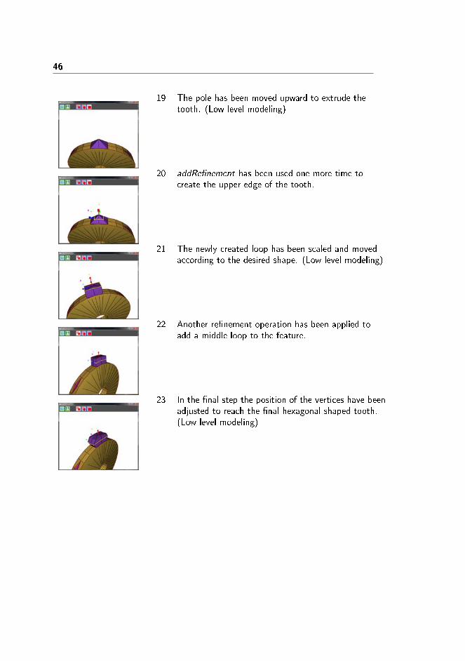
19 The pole has been moved upward to extrude thetooth. (Low level modeling)

20 addRe�nement has been used one more time tocreate the upper edge of the tooth.

21 The newly created loop has been scaled and movedaccording to the desired shape. (Low level modeling)

22 Another re�nement operation has been applied toadd a middle loop to the feature.

23 In the �nal step the position of the vertices have beenadjusted to reach the �nal hexagonal shaped tooth.(Low level modeling)

Chapter 5

Analysis

It is important to test the expressiveness of the modeling system in order to havea better understanding of the limits that a design tool based on polar meshesinvolves. An important set of tests have been performed to compare the power ofthe current modeling system with the SQM algorithm [JAB12] which is in manyways the father of this project. According to Michael Mc Donnell [Don12], SQMsu�ers from some important limitations especially regarding non organic objects.He investigated the limits of the SQM approach de�ning some interesting modelinggoals and evaluating the performances of the SQM algorithm towards them. Healso proposed some extensions to that modeling system in order to improve thoseperformances.

It is interesting at this point to evaluate the behavior of the proposed modelingsystem against the same modeling goals, to visualize the improvements that havebeen reached:

� Modeling of a Lollipop

� Modeling of a Gear

� Modeling of a Ladder

� Modeling of a Head

48 Analysis

Each object will be presented in its desired shape (goal), modeled by SQM, modeledwith the improved SQM from Mc Donnell and �nally modeled using the currentprototype. All screenshot are part of Mc Donnell's work [Don12], expect the onesrelated to the current implementation, of course.

5.1 Lollipop

Figure 5.1: Test result: Lollipop

Figure 5.2: Lollipop: skeleton of the new model

Goal Skeleton (SQM) SQM

5.2 Gear 49

The model produced with SQM is already very close to the goal, but there is stillroom for improvements: the shape of the lollipop is more a drop than a sphere andthe base of the stick isn't perfectly �at [Don12]. These problems aren't related inanyway with the structure of the object and they are di�cult to solve with skeletonbased operations (SQM). The new modeling system overcame easily both of themthanks to low level sculpturing tools that let the designer to de�ne the preciseposition of each individual vertex.

Another problem that a�ects the model produced in SQM is related to the skeletonstructure: in order to use it in future animations, it is important that the skeletonre�ects the structure of the object. Although SQM doesn't provide a method toprocedurally generate a �nal skeleton for the model, it is interesting to notice howthe structure that has been used to produce the mesh, includes quite unnaturally,4 branches to shape the lollipop sphere. The new model, instead, doesn't use anybranch to de�ne the object (in �gure 5.1, the mesh is painted in a single color,therefore it has only one feature) and the entire structure is reduced to a sequenceof skeleton segments, as expected. In this case it is actually possible to use theprocedurally inferred skeleton straight forward in the animation engine.

5.2 Gear

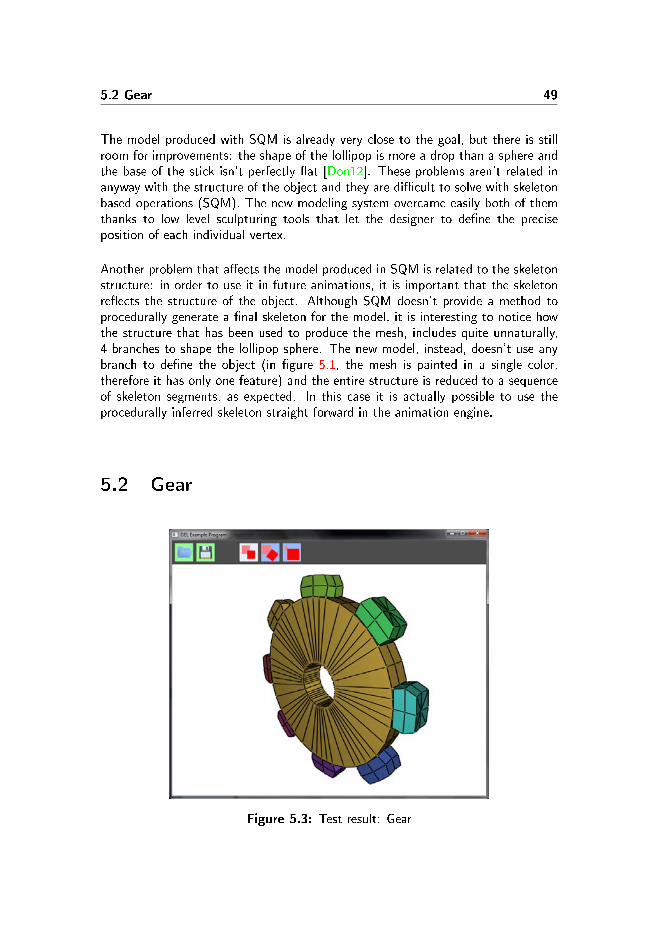
Figure 5.3: Test result: Gear

50 Analysis

(a) Front view (b) Close view

Figure 5.4: Test result: Gear, front, close view and skeleton

Goal SQM Improved SQM

A gear is a good example of inorganic object as it is characterized by sharp edges andlarge �at surfaces. The model produced with SQM is a very pour representation ofthis object, that failed not only in details like the rotation of the gear teeth, but alsoin its basic structure that has been modeled as a pipe, rather than a �at disk. Thisis a general problem in SQM, where the size of the section of a skeleton segmentcan be in�uenced but it isn't practically possible to shape it: although Mc Donnellworked on this aspect providing di�erent types of skeleton nodes, SQM remains verylimited compared to a tool that allow free vertices placement.

Great improvements have been made with the new modeling system, that producesan high quality mesh much closer to the goal and that includes some tiny details likethe hexagonal section of the gear teeth. At a closer look, the new mesh still showssome imperfections, small vertices mispositions that can be easily �xed improving thelow level operations of the prototype, for example including the standard sculpturingtools already available in most commercial software (�rst of all, global and localcoordinate system to move, scale and rotate vertices).

It is also worth to mention that the new model took 10-15 minutes to be completelydeveloped, an amount of e�ort that can be partitioned according to the 80/20 law:the �rst 20% of the time has been spent with high level modeling operations,to de�ne the basic structure of the object, while the remaining 80% has been

5.3 Ladder 51

spent adjusting the individual vertices (low level modeling). SQM is clearly a fasterdevelopment method but, on the other hand, it limits itself to an high level modelingtool and, from this point of view, the e�ort required to produce a complete objectin SQM is comparable to the e�ort spent with high level structural de�nition in thisnew system.

5.3 Ladder

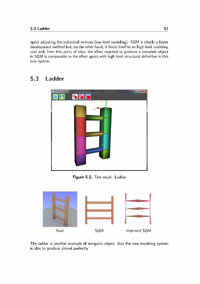
Figure 5.5: Test result: Ladder

Goal SQM Improved SQM

The ladder is another example of inorganic object, that the new modeling systemis able to produce almost perfectly.

52 Analysis

In this case it is interesting to notice how the basic SQM method performs betterthan the improved SQM, which uses di�erent node types to model details like theshape of the rungs section or a �at end in the ladder structure. The reason of thisbehavior is related, one more time, on how mesh details are implemented: in thenew system they are handled with simple vertices displacements, which can't a�ectthe skeleton structure, but in SQM they have to be part of the skeleton and thisclearly interferes with its anatomy.

Another advantage of the new modeling system is the level of detail, which canbe locally controlled in each individual part of the mesh: the ladder produced withSQM has been kept extremely low poly in order to preserve the sharp edges on themain structure, inducing equally raw rungs as well; while the new model is able todi�erentiate these areas and, to some extent, it shows fairly round rungs in a lowpoly support.

5.4 Head

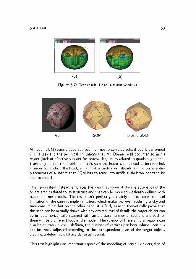
Figure 5.6: Test result: Head

5.4 Head 53

(a) (b)

Figure 5.7: Test result: Head, alternative views

Goal SQM Improved SQM

Although SQM seems a good approach for most organic objects, it poorly performedin this task and the technical limitations that Mc Donnell well documented in hisreport (lack of e�ective support for concavities, issues related to quads alignment..) are only part of the problem: in this case the features that need to be modeled,in order to produce the head, are almost entirely mesh details, simple vertices dis-placements of a sphere that SQM has to force into arti�cial skeleton nodes to beable to model.

The new system instead, embraces the idea that some of the characteristics of theobject aren't related to its structure and that can be more conveniently de�ned withtraditional mesh tools. The result isn't perfect yet, mainly due to some technicallimitation of the current implementation, which make low level modeling tricky andtime consuming, but on the other hand, it is fairly easy to theoretically prove thatthe head can be actually drawn with any desired level of detail: the target object canbe in facts horizontally scanned with an arbitrary number of sections and each ofthem will be a di�erent loop in the model. The valency of these annular regions canalso be arbitrary chosen, de�ning the number of vertices per loop, whose positionscan be freely adjusted according to the correspondent scan of the target object,creating a deformable lattice dense as needed.

This test highlights an important aspect of the modeling of organic objects, �rst of

54 Analysis

all characters: SQM can be used to quickly produce a basic mesh but in practicalcases there are a lot of details that are simply impossible to model with skeletonbones and a completely di�erent approach is necessary. In this perspective, anintegration between a modeling system based on polar meshes and a traditionalsculpturing tool can be an e�ective solution.

5.5 Conclusions

In all the performed tests, the new modeling system produced fairly convincingresults and it was able to overcome the limitations that deeply a�ected the SQMmethod.

The new models contains a richer set of mesh details that they reproduce with more�delity from the desired target object. This has been reached integrating traditionalsculpturing tools (low level modeling) in the polar modeling system, allowing thedesigner to adjust the position of each individual vertex.

This is a feature that SQM isn't able to o�er, not only because its implementationlacks of vertices manipulation tools but also because it is a one way process: inSQM there isn't a bidirectional map between the skeleton and the mesh, thereforeeach adjustment in the structure of the model completely overwrites the entiremodel (Figure 5.8). In the new system instead, the modeling process have beenpushed towards a more AGILE approach where, exploiting the structural informationnaturally embedded in the polar topology, both high and low level operations havebeen speci�cally designed as non disruptive mesh improvements (Figure 5.9).

Skeleton MeshSQMSkeleton design Post process

Figure 5.8: Modeling process of SQM

Mesh

Low levelModeling

-translate-scale-rotate

High levelModeling

- polar refinements- features

Figure 5.9: Modeling process of the new modeling system

Finally, another important improvement that have been reached is related to theskeleton, which now re�ects more naturally the intrinsic structure of the object:SQM uses the skeleton anatomy to include mesh details in the model, but this

55

generates objects with arti�cial and overcomplicated bones structures that are dif-�cult to model and that can't be used for animations without a dramatic (manual)simpli�cation.

The new modeling system moreover, allows any combination of polar and annularregions, providing full native supports to skeletons based on non-simple graphs. Thisovercomes some limitations of SQM that requires tree based skeletons and forcesa branch on the root node, therefore models with loops and holes, like the ladder,can now be shaped in their real structure rather than faked in a post process.

Although in general the new modeling system is a positive proof of concept, it alsoleaves room for some improvements: the low level modeling system needs to beexpanded with the set of tools that already characterize most of commercial 3dsoftware, while symmetric constrains and copy-paste of features can optimize thehigh modeling operations.

56

Part II

Animation

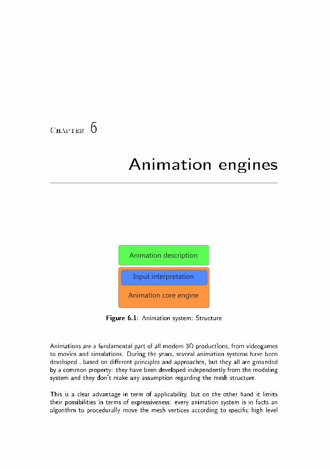
Chapter 6

Animation engines

Animation description

Input interpretation

Animation core engine

Figure 6.1: Animation system: Structure

Animations are a fundamental part of all modern 3D productions, from videogamesto movies and simulations. During the years, several animation systems have beendeveloped , based on di�erent principles and approaches, but they all are groundedby a common property: they have been developed independently from the modelingsystem and they don't make any assumption regarding the mesh structure.

This is a clear advantage in term of applicability, but on the other hand it limitstheir possibilities in terms of expressiveness: every animation system is in facts analgorithm to procedurally move the mesh vertices according to speci�c high level

60 Animation engines

inputs and, from this point of view, animation engines use basic modeling operationsas a low level API library.

It makes sense, at this point, to investigate if a di�erent modeling system can leadto an improved animation engine and if more advanced modeling features can beexploited to implement complex dynamic behaviors.

Conceptually an animation system can be split in two distinct layers: a languageto describe the desired mesh deformation and an internal component that actuallyimplements those behaviors (�gure 6.1).

6.1 Animation description

Animations can be described in several di�erent languages, each of them charac-terized by its own level of details. The most common methods [ana] to describecomplex deformations are:

� Keyframes: an old and simple technique, originally developed in the WaltDisney studios [BW, Las87], where the designer de�nes the poses (verticesposition) in correspondence of speci�c time stamps, called keyframe, that thesystem linearly interpolates in order to approximate the full con�guration setin all the in-between frames.

� Animation scripting languages, where the deformation is de�ned using de-scriptive languages. A typical example of animation scripting is the ImprovSystem [PG96], developed by Ken Perlin and Athomas Goldberg at the MediaResearch Laboratory (New York University).

� Goal directed motions, where the animator specify the desired �nal behaviorand the animation system computes the motion to reach or to performs thatbehavior.

� Motion capture: a physical movement is tracked, recorded and coded intoa virtual animation. In this case the deformation isn't designed in a virtualspace but it is initially performed by an actor, a person or an object, whoactually moves in the real world, while a speci�c system keeps track of themovements with dedicated hardware and software.

For the readers who aren't familiar with them, a more detailed description of thesetechniques can be found in the appendix, including a short discussion on the prosand cons of each method.

6.2 Animation engines 61

6.2 Animation engines

The internal animation engine is where the input is processed and the movementsare performed. The principle itself is very simple: providing an updated position forthe mesh vertices at every screen refresh.

As most of animations aren't described with complete per-frame con�guration sets,interpolation is a fundamental component of every animation engine: in all keyframe based animations, including motion capture, interpolation is obviously nec-essary in order to �ll up the in-betweens, to uniquely de�ne the full con�gurationset for every non-key frame; but interpolation still plays an important role in goaloriented motions and scripted animations, not only because there are cases wherethe dynamic description of the con�guration set is incomplete in some of the times-tamps, but also because the simulation engine that applies physical forces, performsthe dynamic behavior and/or executes the scripts can be independent from the pureanimation engine and it can work on a di�erent rate. For example in Unity3D thephysical simulation is executed at a �xed interval (controlled by the developer),while the animation engine still needs to produce a con�guration set per frame (andthe frame rate isn't controllable by the developer) [unib].

Whatever it has been used to de�ne the motion, key framing rather than a moredynamic description, interpolation isn't a trivial task: in the general case a purelinear interpolation performs poorly and more complex techniques should be usedto convey smoothness and naturalism in the animation. This has been clearlydescribed by John Lasseter in his paper �Principles of traditional animation appliedto 3D computer animation� [Las87], but it is also present in the modern gameindustry that Martin Jonasson and Petri Purho well represent with a famous talkon juicing [jui].

62

Chapter 7

Animation of polar meshes

Obviously the basic structure of a traditional animation system can be applied alsoto polar meshes, but an animation system speci�cally developed for this topologycan exploit some of its properties to gain bene�ts that a more general animationsystem can't o�er.

The most important aspect of polar meshes is the possibility to procedurally infer themesh skeleton from the model with a clear and well structured skinning. This leadsto an animation system that can describe complex animations as a combinationof basic local behaviors, that a�ect singular skeleton nodes without an extensiveknowledge of the entire skeleton structure.

7.1 Inferring the skeleton

The mesh skeleton can be inferred with a fairly simple recursive algorithm, thatperforms a depth-�rst graph visit of the mesh. Variants of this algorithm are alsoused in the selectFeature operation and in the rendering module to highlight di�erentfeatures in di�erent colors.

Although these variants have speci�c per-node operations, the basic recursive struc-

64 Animation of polar meshes

ture is a constant:

SkeletonInit explores the current feature, loop after loop, following a speci�c back-bone. This function relies on skeletonInitLoop and skeletonInitPoleLoop toexplore respectively annular and polar regions. Here new skeleton nodes arecreated and linked to each other.

1 s k e l e t o n I n i t ( Ha l fEdge backboneEdge , Node pa r en t ) :2 Backbone = Loop ( backboneEdge )3 b i = arg ( Backbone , backboneEdge ) // s e t i such as Backbone [ i

]=backboneEdge4 i = b i5 f e a tu r eFound=f a l s e6

7 // boundary l oop f o r ne s t ed f e a t u r e8 i f ( i s P o l e [ v e r t ( opp ( b ) ) ]==0) :9 f o r l i i n Loop ( p rev ( b ) ) :10 p r o c e s s e dVe r t e x [ v e r t ( l i ) ]= t r u e11 c e n t e r s [ v e r t ( l i ) ]= pa r en t12 o f f s e t s [ v e r t ( l i ) ]=pos ( v e r t ( l i ) )−pa r en t . t a r g e t P o s i t i o n13

14 f o r i i n [ b i . . Backbone . l e n gh t ] :15 i f ( f ea tu r eFound ) : break16 Node n = new Node ( )17 parent−>addCh i l d ( n )18 i f ( i s P o l e ( v e r t ( Backbone [ i ] ) ) ) :19 s k e l e t o n I n i t P o l e L o o p ( v e r t ( Backbone [ i ] ) , n )20 break21

22 h = next ( Backbone [ i ] )23 f e a tu r eFound = s k e l e t o n I n i t L o o p (h , n )24 pa r en t = n

SkeletonInitLoop explores a single mesh loop to pair each vertex to its skeletonnode (skinning). Whenever a nested feature is detected, it is queued and laterprocessed with skeletonInit.

1 boo l s k e l e t o n I n i t L o o p ( Hal fEdge loop I tem , Node c u r r e n t ) :2 H = Loop ( l oop I t em )3 f e a tu r eFound=f a l s e4 l i s t n e x tF e a t u r e s5 f o r l i i n H:6 p r o c e s s e dVe r t e x [ v e r t ( l i ) ]= t r u e7 i f ( l i . i s S p l i t ( ) ) :8 f e a tu r eFound=t r u e ;9 r e fBackbone=next ( l i )10 cu r=next ( opp ( re fBackbone ) )11 cu r=next ( opp ( cu r ) )12 whi le ( cu r != re fBackbone ) :13 ne x tF e a t u r e s . push_back ( cu r )14 cu r=next ( opp ( cu r ) )15 cu r=next ( opp ( cu r ) )16

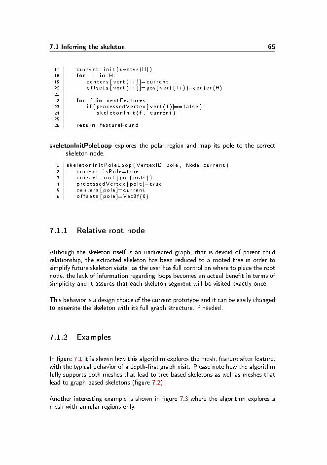
7.1 Inferring the skeleton 65

17 c u r r e n t . i n i t ( c e n t e r (H) )18 f o r l i i n H:19 c e n t e r s [ v e r t ( l i ) ]= c u r r e n t20 o f f s e t s [ v e r t ( l i ) ]=pos ( v e r t ( l i ) )−c e n t e r (H)21

22 f o r f i n ne x tF e a t u r e s :23 i f ( p r o c e s s e dVe r t e x [ v e r t ( f )]== f a l s e ) :24 s k e l e t o n I n i t ( f , c u r r e n t )25

26 re tu rn f e a tu r eFound

skeletonInitPoleLoop explores the polar region and map its pole to the correctskeleton node.

1 s k e l e t o n I n i t P o l e L o o p ( Ver tex ID po le , Node c u r r e n t ) :2 c u r r e n t . i s P o l e=t r u e3 c u r r e n t . i n i t ( pos ( po l e ) )4 p r o c e s s e dVe r t e x [ po l e ]= t r u e5 c e n t e r s [ p o l e ]= c u r r e n t6 o f f s e t s [ p o l e ]=Vec3f (0 )

7.1.1 Relative root node

Although the skeleton itself is an undirected graph, that is devoid of parent-childrelationship, the extracted skeleton has been reduced to a rooted tree in order tosimplify future skeleton visits: as the user has full control on where to place the rootnode, the lack of information regarding loops becomes an actual bene�t in terms ofsimplicity and it assures that each skeleton segment will be visited exactly once.

This behavior is a design choice of the current prototype and it can be easily changedto generate the skeleton with its full graph structure, if needed.

7.1.2 Examples

In �gure 7.1 it is shown how this algorithm explores the mesh, feature after feature,with the typical behavior of a depth-�rst graph visit. Please note how the algorithmfully supports both meshes that lead to tree-based skeletons as well as meshes thatlead to graph-based skeletons (�gure 7.2).

Another interesting example is shown in �gure 7.3 where the algorithm explores amesh with annular regions only.

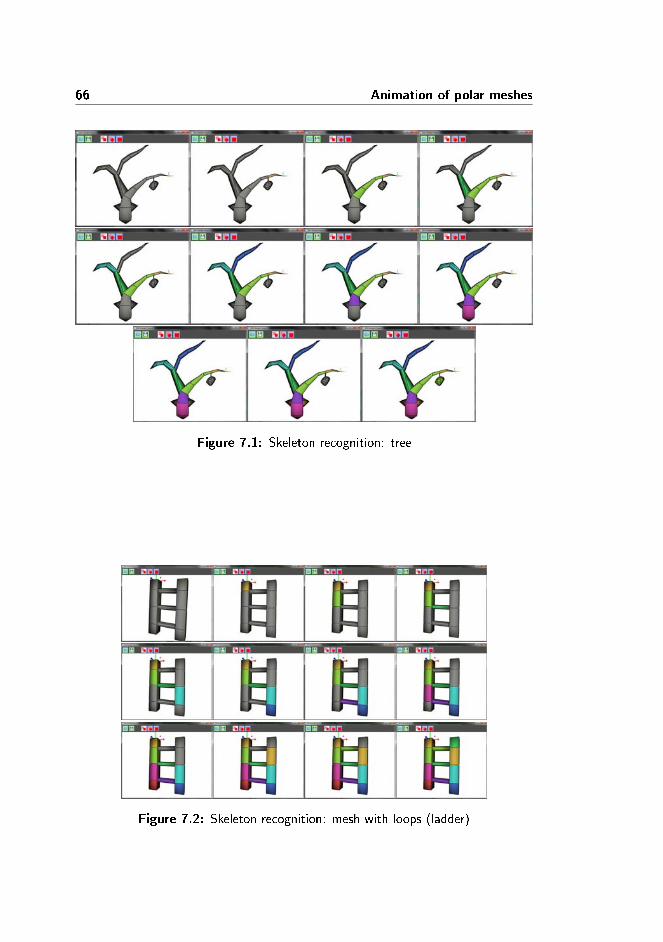
66 Animation of polar meshes

Figure 7.1: Skeleton recognition: tree

Figure 7.2: Skeleton recognition: mesh with loops (ladder)

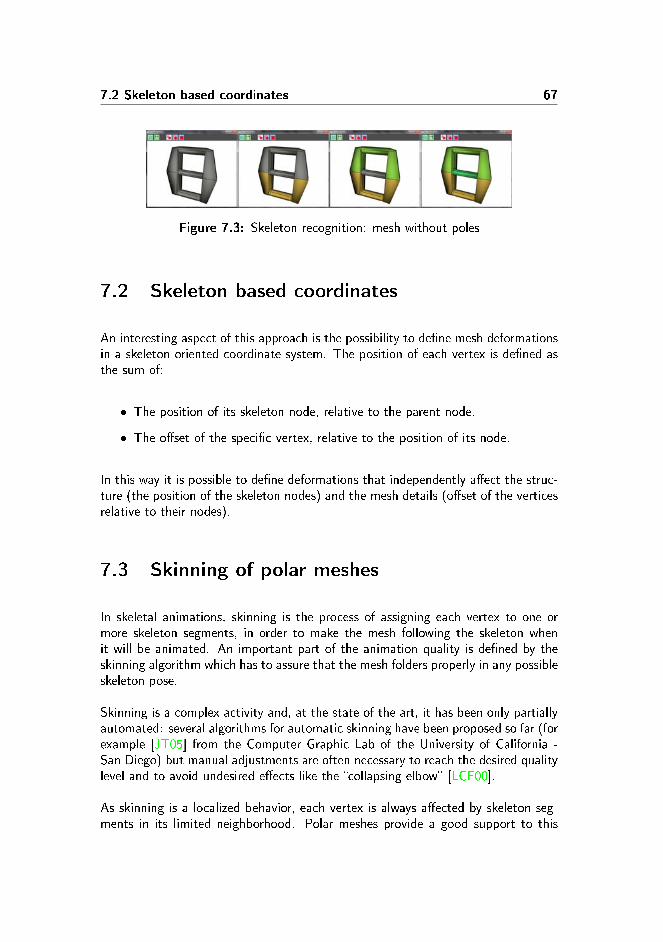
7.2 Skeleton based coordinates 67

Figure 7.3: Skeleton recognition: mesh without poles

7.2 Skeleton based coordinates

An interesting aspect of this approach is the possibility to de�ne mesh deformationsin a skeleton oriented coordinate system. The position of each vertex is de�ned asthe sum of:

� The position of its skeleton node, relative to the parent node.

� The o�set of the speci�c vertex, relative to the position of its node.

In this way it is possible to de�ne deformations that independently a�ect the struc-ture (the position of the skeleton nodes) and the mesh details (o�set of the verticesrelative to their nodes).

7.3 Skinning of polar meshes

In skeletal animations, skinning is the process of assigning each vertex to one ormore skeleton segments, in order to make the mesh following the skeleton whenit will be animated. An important part of the animation quality is de�ned by theskinning algorithm which has to assure that the mesh folders properly in any possibleskeleton pose.

Skinning is a complex activity and, at the state of the art, it has been only partiallyautomated: several algorithms for automatic skinning have been proposed so far (forexample [JT05] from the Computer Graphic Lab of the University of California -San Diego) but manual adjustments are often necessary to reach the desired qualitylevel and to avoid undesired e�ects like the �collapsing elbow� [LCF00].

As skinning is a localized behavior, each vertex is always a�ected by skeleton seg-ments in its limited neighborhood. Polar meshes provide a good support to this

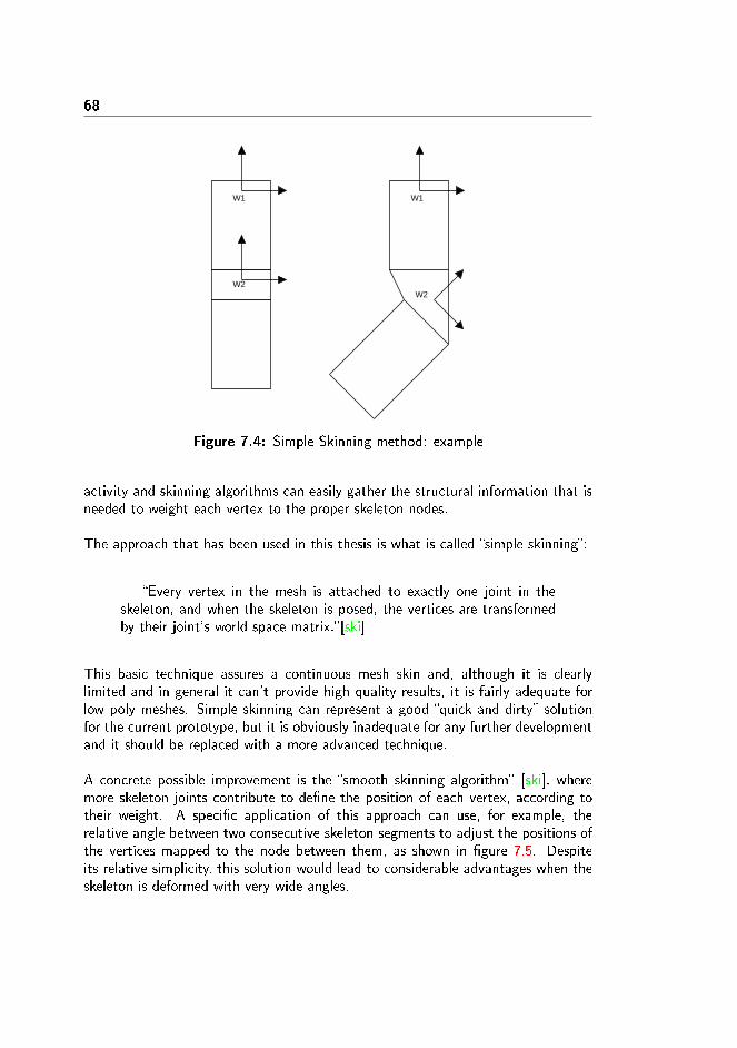
68

W1

W2

W1

W2

Figure 7.4: Simple Skinning method: example

activity and skinning algorithms can easily gather the structural information that isneeded to weight each vertex to the proper skeleton nodes.

The approach that has been used in this thesis is what is called �simple skinning�:

�Every vertex in the mesh is attached to exactly one joint in theskeleton, and when the skeleton is posed, the vertices are transformedby their joint's world space matrix.�[ski]

This basic technique assures a continuous mesh skin and, although it is clearlylimited and in general it can't provide high quality results, it is fairly adequate forlow poly meshes. Simple skinning can represent a good �quick and dirty� solutionfor the current prototype, but it is obviously inadequate for any further developmentand it should be replaced with a more advanced technique.

A concrete possible improvement is the �smooth skinning algorithm� [ski], wheremore skeleton joints contribute to de�ne the position of each vertex, according totheir weight. A speci�c application of this approach can use, for example, therelative angle between two consecutive skeleton segments to adjust the positions ofthe vertices mapped to the node between them, as shown in �gure 7.5. Despiteits relative simplicity, this solution would lead to considerable advantages when theskeleton is deformed with very wide angles.

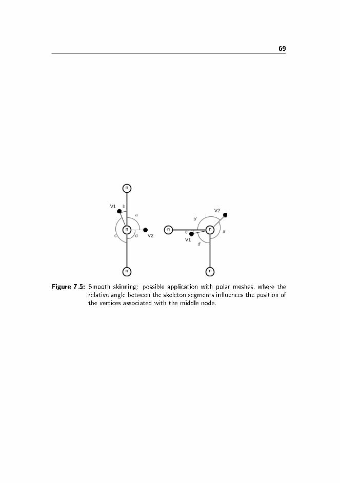
69

a

b

c da’

b’

c’

d’

V1

V2V1

V2

n

n

n

nn

n

Figure 7.5: Smooth skinning: possible application with polar meshes, where therelative angle between the skeleton segments in�uences the position ofthe vertices associated with the middle node.

70

Chapter 8

Implementation

In the prototype a small animation system has been implemented, in order to demon-strate the applicability of some of the techniques that have been described as well asto investigate the advantages of the usage of polar meshes regarding the animationdevelopment. This isn't a complete engine, and it isn't intended to be used in realproductions, but it will show some of the possibilities o�ered by the new modelingsystem.

8.1 The prototype

From a more technical prospective it has been implemented a behavior based ani-mation system, where the �nal deformation is de�ned as a combination of a variablenumber of simpler behaviors.

Although these behaviors have been hard coded in the current prototype, the struc-ture of the engine is already oriented towards a plug-in based animation system andit will be fairly easy in the future to add a script engine to the system. In this waythe designer will be able to dynamically de�ne new behaviors via scripts or graphicaltools.

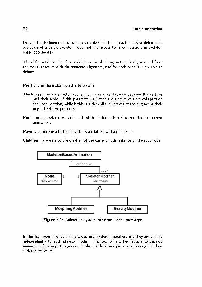
72 Implementation

Despite the technique used to store and describe them, each behavior de�nes theevolution of a single skeleton node and the associated mesh vertices in skeletonbased coordinates.

The deformation is therefore applied to the skeleton, automatically inferred fromthe mesh structure with the standard algorithm, and for each node it is possible tode�ne:

Position: in the global coordinate system

Thickness: the scale factor applied to the relative distance between the verticesand their node. If this parameter is 0 then the ring of vertices collapses onthe node position, while if this is 1 then all the vertices of the ring are at theiroriginal relative positions.

Root node: a reference to the node of the skeleton de�ned as root for the currentanimation.

Parent: a reference to the parent node relative to the root node

Children: reference to the children of the current node, relative to the root node

NodeSkeleton node

SkeletonBasedAnimation

SkeletonModifierBasic modifier

MorphingModifier GravityModifier

1 1

Animation1

1..*

Figure 8.1: Animation system: structure of the prototype

In this framework, behaviors are coded into skeleton modi�ers and they are appliedindependently to each skeleton node. This locality is a key feature to developanimations for completely general meshes, without any previous knowledge on theirskeleton structure.

73

Each skeleton node can be deformed by a list of di�erent modi�ers, that are se-quentially applied to de�ne its �nal position: at each iteration, a general modi�erin the list receives in input the position of the current node, deformed by all theprevious behaviors, and it outputs its updated position to the modi�er that follows.

Finally the complete animation is the global combination of these local simple be-haviors.

74

Chapter 9

Analysis

In order to demonstrate the opportunities o�ered by an animation system completelytailored on polar meshes, few examples has been developed:

Morphing: the animation simulates the growing process of plants, making the meshgrowing from the root node.

Gravity deforms the mesh in order to simulate the e�ect of the gravity. In thisprocess the root node is considered �xed, while the rest of the mesh bendsunder the force.

9.1 Morphing

Morphing, an animation that changes the shape of the object, is typically unsup-ported by traditional skeleton based engines and in general it requires a completelydi�erent animation system. A particularly interesting example of morphing is plantdevelopment, the animation that simulates the biological growing process of weedsand trees, where morphing techniques are often mixed with traditional skeletonbased transformations.

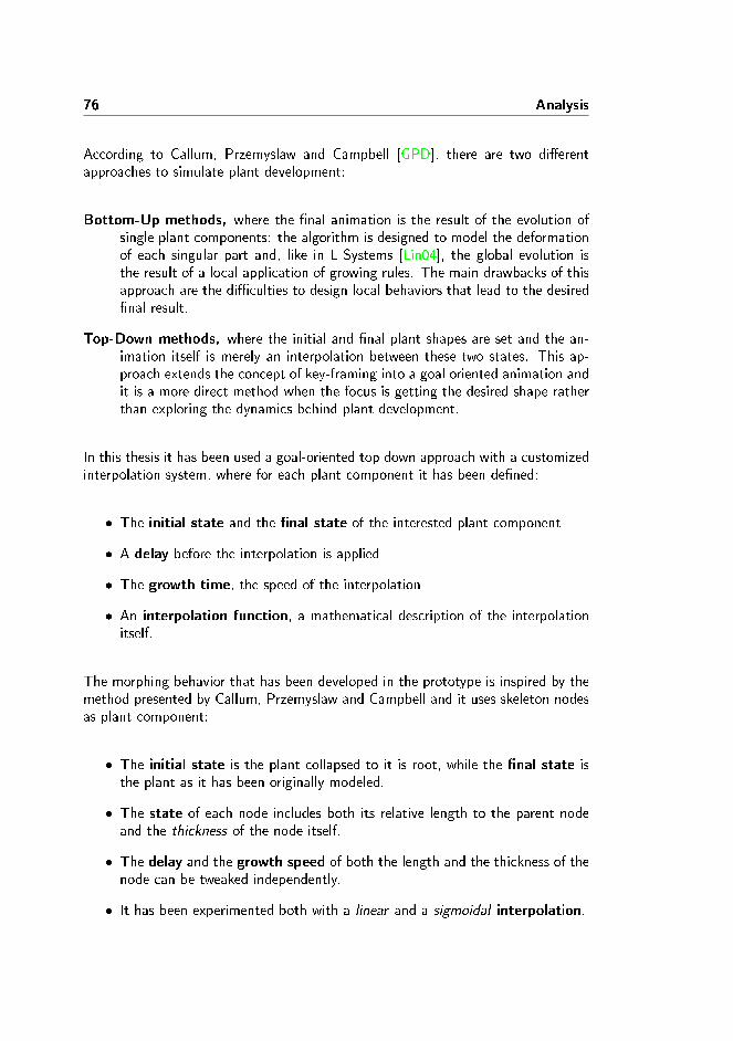
76 Analysis

According to Callum, Przemyslaw and Campbell [GPD], there are two di�erentapproaches to simulate plant development:

Bottom-Up methods, where the �nal animation is the result of the evolution ofsingle plant components: the algorithm is designed to model the deformationof each singular part and, like in L-Systems [Lin04], the global evolution isthe result of a local application of growing rules. The main drawbacks of thisapproach are the di�culties to design local behaviors that lead to the desired�nal result.

Top-Down methods, where the initial and �nal plant shapes are set and the an-imation itself is merely an interpolation between these two states. This ap-proach extends the concept of key-framing into a goal oriented animation andit is a more direct method when the focus is getting the desired shape ratherthan exploring the dynamics behind plant development.

In this thesis it has been used a goal-oriented top down approach with a customizedinterpolation system, where for each plant component it has been de�ned:

� The initial state and the �nal state of the interested plant component

� A delay before the interpolation is applied

� The growth time, the speed of the interpolation

� An interpolation function, a mathematical description of the interpolationitself.

The morphing behavior that has been developed in the prototype is inspired by themethod presented by Callum, Przemyslaw and Campbell and it uses skeleton nodesas plant component:

� The initial state is the plant collapsed to it is root, while the �nal state isthe plant as it has been originally modeled.

� The state of each node includes both its relative length to the parent nodeand the thickness of the node itself.

� The delay and the growth speed of both the length and the thickness of thenode can be tweaked independently.

� It has been experimented both with a linear and a sigmoidal interpolation.

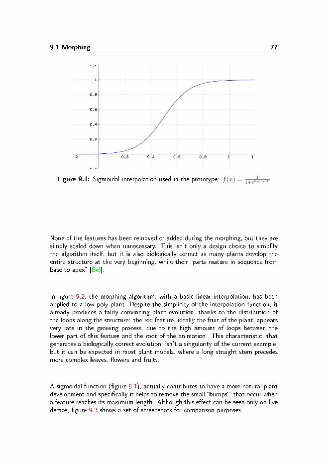
9.1 Morphing 77

Figure 9.1: Sigmoidal interpolation used in the prototype: f(x) = 11+e5−x∗10

None of the features has been removed or added during the morphing, but they aresimply scaled down when unnecessary. This isn't only a design choice to simplifythe algorithm itself, but it is also biologically correct as many plants develop theentire structure at the very beginning, while their �parts mature in sequence frombase to apex� [Bel].

In �gure 9.2, the morphing algorithm, with a basic linear interpolation, has beenapplied to a low poly plant. Despite the simplicity of the interpolation function, italready produces a fairly convincing plant evolution, thanks to the distribution ofthe loops along the structure: the red feature, ideally the fruit of the plant, appearsvery late in the growing process, due to the high amount of loops between thelower part of this feature and the root of the animation. This characteristic, thatgenerates a biologically correct evolution, isn't a singularity of the current example,but it can be expected in most plant models, where a long straight stem precedesmore complex leaves, �owers and fruits.

A sigmoidal function (�gure 9.1), actually contributes to have a more natural plantdevelopment and speci�cally it helps to remove the small �bumps�, that occur whena feature reaches its maximum length. Although this e�ect can be seen only on livedemos, �gure 9.3 shows a set of screenshots for comparison purposes.

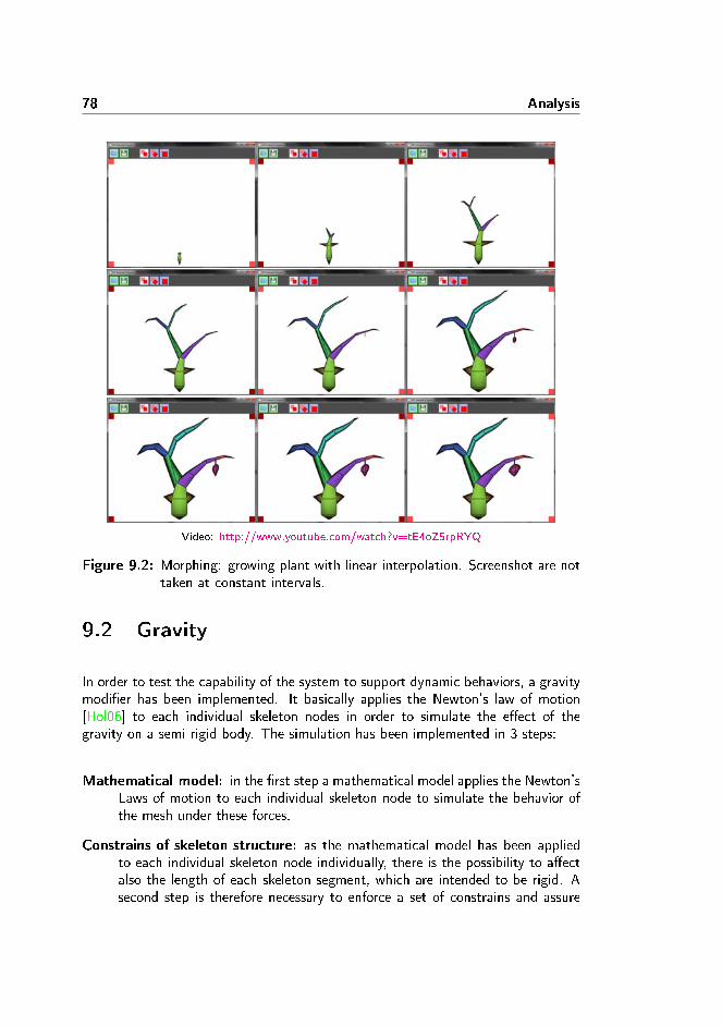
78 Analysis

Video: http://www.youtube.com/watch?v=tE4oZ5rpRYQ

Figure 9.2: Morphing: growing plant with linear interpolation. Screenshot are nottaken at constant intervals.

9.2 Gravity

In order to test the capability of the system to support dynamic behaviors, a gravitymodi�er has been implemented. It basically applies the Newton's law of motion[Hol06] to each individual skeleton nodes in order to simulate the e�ect of thegravity on a semi rigid body. The simulation has been implemented in 3 steps:

Mathematical model: in the �rst step a mathematical model applies the Newton'sLaws of motion to each individual skeleton node to simulate the behavior ofthe mesh under these forces.

Constrains of skeleton structure: as the mathematical model has been appliedto each individual skeleton node individually, there is the possibility to a�ectalso the length of each skeleton segment, which are intended to be rigid. Asecond step is therefore necessary to enforce a set of constrains and assure

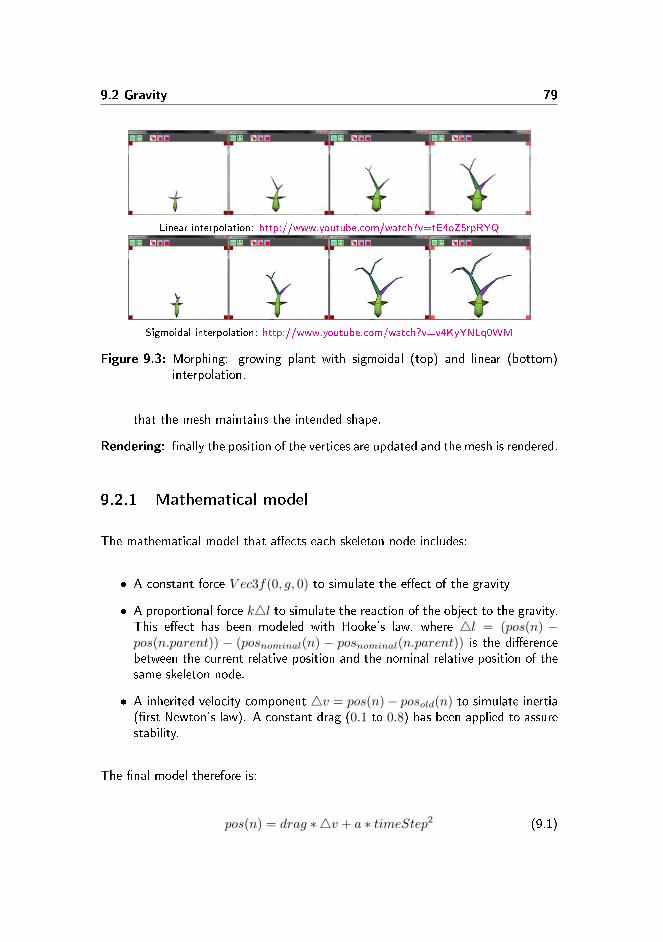
9.2 Gravity 79

Linear interpolation: http://www.youtube.com/watch?v=tE4oZ5rpRYQ

Sigmoidal interpolation: http://www.youtube.com/watch?v=v4KyYNLq0WM

Figure 9.3: Morphing: growing plant with sigmoidal (top) and linear (bottom)interpolation.

that the mesh maintains the intended shape.

Rendering: �nally the position of the vertices are updated and the mesh is rendered.

9.2.1 Mathematical model

The mathematical model that a�ects each skeleton node includes:

� A constant force V ec3f(0, g, 0) to simulate the e�ect of the gravity

� A proportional force k4l to simulate the reaction of the object to the gravity.This e�ect has been modeled with Hooke's law, where 4l = (pos(n) −pos(n.parent)) − (posnominal(n) − posnominal(n.parent)) is the di�erencebetween the current relative position and the nominal relative position of thesame skeleton node.

� A inherited velocity component 4v = pos(n)− posold(n) to simulate inertia(�rst Newton's law). A constant drag (0.1 to 0.8) has been applied to assurestability.

The �nal model therefore is:

pos(n) = drag ∗ 4v + a ∗ timeStep2 (9.1)

80 Analysis

a = V ec3f(0, g, 0) + k4l (9.2)

9.2.2 Constrains of skeleton structure

One of the consequences to apply the mathematical model to each skeleton nodeindividually, it is the possibility to a�ect also the length of each skeleton segment.Although the structure can blend under the gravity, the skeleton segments are in-tended to be rigid and they aren't supposed to change their length.

This can be enforced using the same relaxation technique that Thomas Jakobsenpresented in its paper �Advanced Character Physics� [Jak01] to solve multiple con-strains for a set of particles.

�A common model for cloth consists of a simple system of intercon-nected springs and particles. However, it is not always trivial to solve thecorresponding system of di�erential equations. It su�ers from some ofthe same problems as the penalty-based systems: Strong springs leadsto sti� systems of equations that lead to instability if only simple inte-gration techniques are used, or at least bad performance � which leadsto pain. Conversely, weak springs lead to elastically looking cloth.

However, an interesting thing happens if we let the sti�ness of thesprings go to in�nity: The system suddenly becomes solvable in a stableway with a very simple and fast approach.�[Jak01]

The key idea here is iterating multiple times over each individual constrain untilthe system reaches the desired level of stability. One of the interesting aspect ofthis technique is that it always hits a good compromise between performances andquality: in the current implementation for example each constrain has been relaxed10 time, a number that in most cases leads to good looking animations, but when itis insu�cient the animation will look a bit less clean without any disruptive resultsboth quality and performance wise.

9.2.3 Rendering

In the last phase, the new vertices positions are applied and the rendering is per-formed.

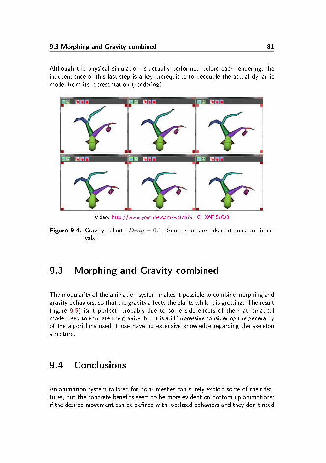
9.3 Morphing and Gravity combined 81

Although the physical simulation is actually performed before each rendering, theindependence of this last step is a key prerequisite to decouple the actual dynamicmodel from its representation (rendering).

Video: http://www.youtube.com/watch?v=C_X6Rl5rCs0

Figure 9.4: Gravity: plant. Drag = 0.1. Screenshot are taken at constant inter-vals.

9.3 Morphing and Gravity combined

The modularity of the animation system makes it possible to combine morphing andgravity behaviors, so that the gravity a�ects the plants while it is growing. The result(�gure 9.5) isn't perfect, probably due to some side e�ects of the mathematicalmodel used to emulate the gravity, but it is still impressive considering the generalityof the algorithms used, those have no extensive knowledge regarding the skeletonstructure.

9.4 Conclusions

An animation system tailored for polar meshes can surely exploit some of their fea-tures, but the concrete bene�ts seem to be more evident on bottom-up animations:if the desired movement can be de�ned with localized behaviors and they don't need

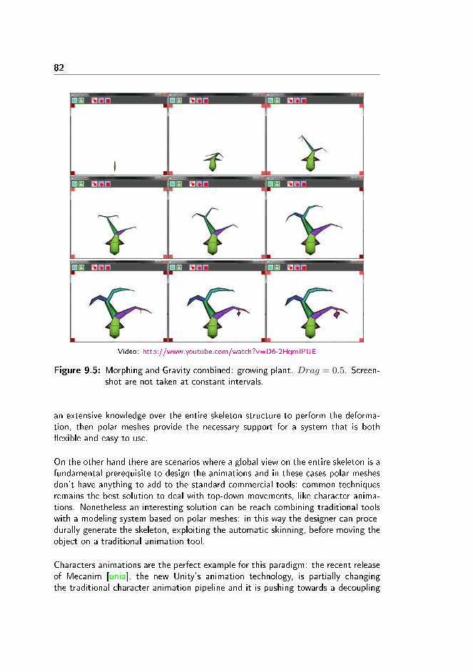
82

Video: http://www.youtube.com/watch?v=D6-2HqmIPUE

Figure 9.5: Morphing and Gravity combined: growing plant. Drag = 0.5. Screen-shot are not taken at constant intervals.

an extensive knowledge over the entire skeleton structure to perform the deforma-tion, then polar meshes provide the necessary support for a system that is both�exible and easy to use.

On the other hand there are scenarios where a global view on the entire skeleton is afundamental prerequisite to design the animations and in these cases polar meshesdon't have anything to add to the standard commercial tools: common techniquesremains the best solution to deal with top-down movements, like character anima-tions. Nonetheless an interesting solution can be reach combining traditional toolswith a modeling system based on polar meshes: in this way the designer can proce-durally generate the skeleton, exploiting the automatic skinning, before moving theobject on a traditional animation tool.

Characters animations are the perfect example for this paradigm: the recent releaseof Mecanim [unia], the new Unity's animation technology, is partially changingthe traditional character animation pipeline and it is pushing towards a decoupling

83

between the character design and the animations design, in such a way that it is nowpossible to apply a broad class of humanoid animations to any humanoid characters.In this context it is important to exploit the existing animation database and to doso it is necessary to export skinned characters with a skeleton as close as possibleto the standardized one.

It is clearly possible to develop a tool for generating the traditional bones structure,for procedurally skinning the mesh to it and, with a bit more e�ort, to automaticallysimplify the skeleton structure to make it �ts the standard avatar. This mixed ap-proach, between polar meshes and traditional software, has already been suggestedby some Unity game designers, and probably it is the best way to publish a �rstcommercial tool strongly based on polar meshes.

84

Part III

Procedurally generatedcontent

Chapter 10

L-Systems

10.1 Introduction to L-Systems

Lindenmayer systems or L-Systems are a mathematical description of the develop-ment process of organic structures. Originally developed by Lindenmayer in 1968[Lin68], this method has been initially applied to model the behavior of simple mul-ticellular organisms and later it became one of the key modeling tools to describethe growing process of plants and trees.

L-Systems represents the object as a string of symbols, which are iteratively replacedapplying a set of production rules in order to make the object evolving [Lin04]. It isimportant to note that in each iteration all the symbol replacements are concurrentlyapplied, to simulate the biological evolution of the organic model at cellular level. Asillustrative example the production A→ AB applied to the initial string ABBAABgenerates ABBBABABB in output.

Technically L-Systems are strongly based on the formal language theory and theycan be de�ned with the grammar L =< V,w, P >, characterized by:

� An alphabet V , where:

� V ∗ is the set of words over V

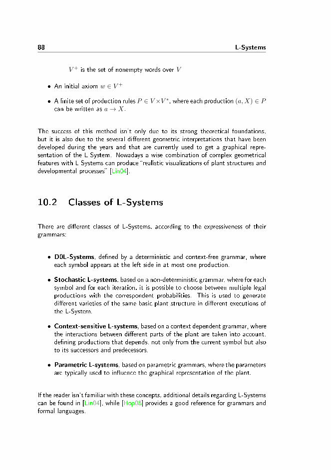
88 L-Systems

� V + is the set of nonempty words over V

� An initial axiom w ∈ V +

� A �nite set of production rules P ∈ V ×V ∗, where each production (a,X) ∈ Pcan be written as a→ X.

The success of this method isn't only due to its strong theoretical foundations,but it is also due to the several di�erent geometric interpretations that have beendeveloped during the years and that are currently used to get a graphical repre-sentation of the L-System. Nowadays a wise combination of complex geometricalfeatures with L-Systems can produce �realistic visualizations of plant structures anddevelopmental processes� [Lin04].

10.2 Classes of L-Systems

There are di�erent classes of L-Systems, according to the expressiveness of theirgrammars:

� D0L-Systems, de�ned by a deterministic and context-free grammar, whereeach symbol appears at the left side in at most one production.

� Stochastic L-systems, based on a non-deterministic grammar, where for eachsymbol and for each iteration, it is possible to choose between multiple legalproductions with the correspondent probabilities. This is used to generatedi�erent varieties of the same basic plant structure in di�erent executions ofthe L-System.

� Context-sensitive L-systems, based on a context dependent grammar, wherethe interactions between di�erent parts of the plant are taken into account,de�ning productions that depends, not only from the current symbol but alsoto its successors and predecessors.

� Parametric L-systems, based on parametric grammars, where the parametersare typically used to in�uence the graphical representation of the plant.

If the reader isn't familiar with these concepts, additional details regarding L-Systemscan be found in [Lin04], while [Hop08] provides a good reference for grammars andformal languages.

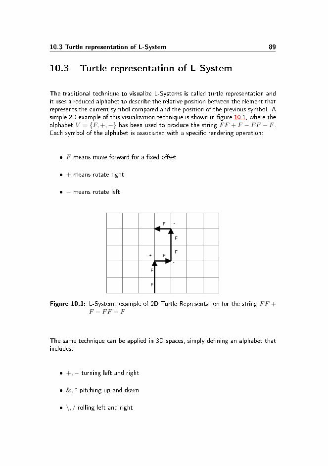
10.3 Turtle representation of L-System 89

10.3 Turtle representation of L-System

The traditional technique to visualize L-Systems is called turtle representation andit uses a reduced alphabet to describe the relative position between the element thatrepresents the current symbol compared and the position of the previous symbol. Asimple 2D example of this visualization technique is shown in �gure 10.1, where thealphabet V = {F,+,−} has been used to produce the string FF + F − FF − F .Each symbol of the alphabet is associated with a speci�c rendering operation:

� F means move forward for a �xed o�set

� + means rotate right

� − means rotate left

F

F

FF

F

F

+

-

-

Figure 10.1: L-System: example of 2D Turtle Representation for the string FF +F − FF − F

The same technique can be applied in 3D spaces, simply de�ning an alphabet thatincludes:

� +,− turning left and right

� &, � pitching up and down

� \, / rolling left and right

90 L-Systems

Figure 10.2: L-System: interpretation of alphabet for 3D turtle representation(source: [Lin04])

Finally, the turtle representation can be also expanded to support the branchingstructures of axial trees. This can be easily done using a stack and introducing twomore symbols in the alphabet:

� [ creates a branch at the current position, pushing the state on the stack.

� ] moves the rendering back to the previous branch point, restoring the statefrom the stack (pop)

A couple of very simple 2D examples are shown in �gure 10.3.

F

F

+F-FF

F

F

F+F

-FF

F +F -FF

(a) String: FF [+F ][−F + FF ] (b) String: FF [+F − F [+F − F ]F ]FF

Figure 10.3: L-System: examples of 2D Turtle Representation with branches

10.4 L-System and polar meshes 91

10.4 L-System and polar meshes

Polar meshes are a good graphical tool to visualize L-Systems and they can easilyproduce fairly complex graphical interpretations with a relative small e�ort: eachsegment of a turtle based L-System can be mapped into a di�erent (set of) featurein the polar mesh, while the branching structure is ensured by the capability ofprocedurally generate nested features.

As it has been discussed in depth above, skeleton branches are strictly de�ned inpolar meshes and they are implemented with a clear, deterministic and well organizedmesh topology. This unique characteristic of polar meshes is a key factor to keepthe rendering operation simple and ensuring an high quality mesh, independently ofthe relative angle between the skeleton segments involved in the branch.

92

Chapter 11

Implementation

In order to evaluate and test the usage of polar meshes in this frame, a context-free, stochastic and parametric L-System has been integrated in the prototype. Thecurrent implementation is intended to be a simple proof of concept and it is in factsa�ected by several limitations, the most critical one is maybe the lack of real timestring parser for L-Systems that forces the production rules to be hard-coded in theprototype.

The L-System that has been implemented uses a turtle-like graphical representation,where each symbol describe the behavior of a speci�c skeleton segment:

� Alphabet V = {P,L, L0, [L, LR, ]}, where

� P moves forward and draws a pole

� L moves forward and draws a simple loop

� L0moves forward and draws a simple loop that can eventually be replaced(see productions)

� [L moves forward, it pushes the state on the stack, and it creates anested feature on the left, drawing a loop to support it.

� [R moves forward, it pushes the state on the stack, and it creates anested feature on the right, drawing a loop to support it.

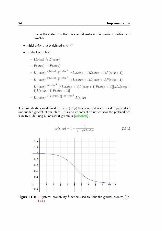
94 Implementation

� ] pops the state from the stack and it restores the previous position anddirection

� Initial axiom: user de�ned w ∈ V +

� Production rules:

� L(step)1→ L(step)

� P (step)1→ P (step)

� L0(step)pr(step)−pr(step)2→ [LL0(step+ 1)L(step+ 1)P (step+ 1)]

� L0(step)pr(step)−pr(step)2→ [RL0(step+ 1)L(step+ 1)P (step+ 1)]

� L0(step)pr(step)2→ [LL0(step + 1)L(step + 1)P (step + 1)][RL0(step +

1)L(step+ 1)P (step+ 1)]

� L0(step)1−2∗pr(step)+pr(step)2→ L(step)

The probabilities are de�ned by the pr(step) function, that is also used to prevent anunbounded growth of the plant. It is also important to notice how the probabilitiessum to 1, de�ning a consistent grammar [odAtD94].

pr(step) = 1− 1

1 + e5.2−step(11.1)

Figure 11.1: L-System: probability function used to limit the growth process (Eq.11.1)

11.1 Implicit string representation and real time mesh operations 95

Similar functions have also been applied to adjust length and thickness of the fea-tures from the root to the leafs of the plant (Eq. 11.2). Sigmoidal functions aregood approximations of a wide range of biological growing processes, where �theinitial part of the curve represents the growth of a young organism, while the latterpart corresponds to the organism close to its �nal size� [Lin04] and they can beeasily implemented exploiting the parametric nature of the underlying grammar.

L = 1− 1

1 + e2−step(11.2)

11.1 Implicit string representation and real time

mesh operations

Usually L-Systems produces an explicit string of symbols that is later converted inits graphical representation often with o�ine methods, but in this prototype it hasbeen implemented a di�erent approach: polar meshes contain by themselves enoughstructural information to completely avoid any explicit symbol representation andto apply the productions directly to the mesh, in real time. In this case the meshitself can be considered the direct output of the L-System, where loops representsymbols and backbones represent the string structure.

In this framework, the productions have been coded as a sequence of polar meshoperations, a procedural application of the same modeling tools that have alreadybeen presented in the �rst part of this report. This is a powerful approach thatcan be used, in the future, to develop more advanced tools, where procedurallygenerated L-Systems may use variants of a manually de�ned feature.

96

Chapter 12

Analysis

Despite it is just a proof of concept, this prototype already produces fairly goodresults (Figure 12.1): the feature nesting is smooth and clean, it doesn't presentany singularity and the level of details is adjusted in real-time, a�ecting only alocalized area of the mesh and making sure that new features can always be added.

On the other hand, the prototype is a�ected by several limitations, due to both thecurrent implementation as well as some speci�c characteristics of the method itself.

The �rst comment is regarding the current branching behavior that produces nestedfeatures always from the side of the parent feature, which doesn't continue to growafter the branch. This is a design choice that has been made because of its simplicityand it is the actual reason why the �nal plant looks more like a shrub than a tree,but it can be easily changed.

A deeper problem that isn't easy to �x instead, is the lack of direction: in order tonest a new feature on an existing loop, it is necessary to de�ne which vertices ofthe loop will be a�ected by the nesting operation, but selecting the right verticesin order to have the gap oriented into a particular direction, isn't a trivial task andbrute forcing seems to be the only way to chose an optimal solution.

It is interesting to notice how this problem isn't due to any speci�c detail of thecurrent implementation but it is instead a consequence of the usage of polar meshes:

98 Analysis

Figure 12.1: L-System: example.

they do support mesh operations that directly a�ect (or that are a�ected by) theskeleton, but any structural information needs to be inferred in real time and this iscomputationally heavy.

The system is, in facts, already a�ected by performance issues, that can be easilyseen removing the stochastic branching limitation and allowing the generation oftwo nested features at each iteration. Figure 12.2 is an example that took severalseconds to be computed and in 11 iterations it becomes so time consuming to reachthe boundaries of what it is usually considered real-time.

The pro�ler used for a deeper analysis revealed that most of the e�ort is partitionedbetween the actual generation of the new features (20%) and the updates of therendering data (44%), where most of the time (34% out of 44%) is actually spentcomputing the new per-vertex normals.

Although the code isn't completely optimized it is clear that a drastic reduction ofthe overall e�ort is impossible and the theory of computational complexity actuallysupports this conclusion: although each feature requires roughly the same e�ort

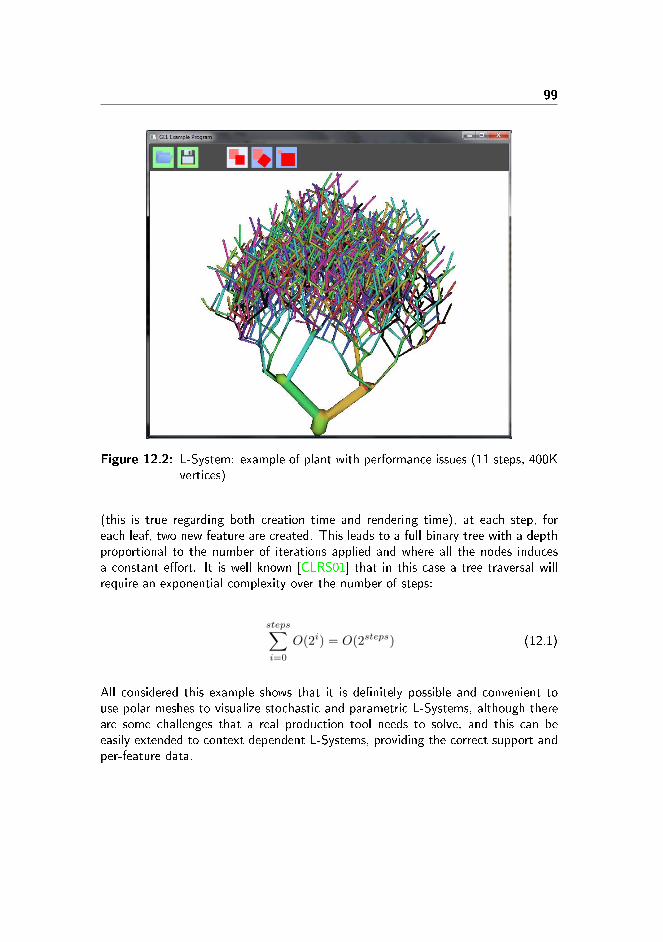
99

Figure 12.2: L-System: example of plant with performance issues (11 steps, 400Kvertices)

(this is true regarding both creation time and rendering time), at each step, foreach leaf, two new feature are created. This leads to a full binary tree with a depthproportional to the number of iterations applied and where all the nodes inducesa constant e�ort. It is well known [CLRS01] that in this case a tree traversal willrequire an exponential complexity over the number of steps:

steps∑i=0

O(2i) = O(2steps) (12.1)

All considered this example shows that it is de�nitely possible and convenient touse polar meshes to visualize stochastic and parametric L-Systems, although thereare some challenges that a real production tool needs to solve, and this can beeasily extended to context dependent L-Systems, providing the correct support andper-feature data.

100

Part IV

Conclusions

Chapter 13

Conclusions

As presented in the �rst part of the report, the main goal of this project wasevaluating the potential of a modeling system based on polar meshes, in relation tomodeling, animations and procedurally generated content.

Modeling

From the modeling point of view, this project can be seen as an evolution of SQMand it is interesting to compare the new system with this older method. In histhesis Mc Donnell [Don12] showed that SQM has a limited expressiveness and onlya narrow range of shapes can be conveniently modeled with this technique. This ismainly because in SQM the �nal vertices positions aren't controlled by the designerbut they are inferred from the skeleton structure.

In the current modeling system, these limitation have been completely overcomeand it is now possible to model any arbitrary shape as long as it leads to a closedmesh. This has been reached allowing the user to de�ne the exact position of eachindividual vertex (low level modeling) as well as with a deeper understanding of theconcept of polar mesh: in the new system any combination of polar and annularregions is allowed and it leads to a mesh structure that is no longer based on arooted tree (an important detail in the implementation of the SQM method) but

104 Conclusions

that now supports the generality of a non-simple graph (high level modeling).

This new modeling system can be de�nitely exploited to push the development of3D assets into a more AGILE process and to some extent this is already supportedin the prototype, but on the other hand the current implementation doesn't seemto provide a fair platform for a fast-paced designing process: the actual modelingstill feels quite clumsy, mainly due to the poor GUI and limited low-level modelingtools. In this perspective an integration with a traditional 3D software can actuallyimprove the user experience and provide a better support for the low level modeling.

Animations

One of the key characteristics of polar meshes is their implicit skeleton which canbe inferred in real time from the topological structure of the mesh and that can beused to design more �exible animations. In this project a behavior based animationengine has been developed, where the mesh skeleton is automatically gathered anddeformed according to the desired movement.

This approach turned out to be very e�ective for bottom-up animations, such asmorphing, physically based motion and whenever the global movement is de�nedas a combination of local behaviors a�ecting each skeleton node individually; butit doesn't seem to help when an extensive knowledge on the entire skeleton struc-ture is needed, like in humanoid animations. In these situations polar meshes stillrepresent a valid modeling tool and they can always be used to procedurally gener-ate the skeleton structure, but this topology doesn't lead to any real improvementsanimations wise.

Finally, polar meshes seems to provide a fairly good support for skinning algorithms,that typically correlate each vertex with skeleton nodes in a limited neighborhood,and further developments can actually provide a better overview of the potential ofpolar meshes in this sense.

Procedurally generated content

In principle a procedurally generated content is no more than a repeatable sequenceof API calls, either related to modeling and/or animations. In this project it hasbeen implemented an L-System to demonstrate the applicability of this principle topolar meshes and to evaluate to what extent polar mesh operations can be used ascoherent and invokable API.

105

The outcomes show that it is de�nitely possible to automate sequences of mesh op-erations and polar meshes provide a really good support for procedurally generatedcontent that massively a�ects the model structure: usually L-Systems are designedto produce an explicit string of symbols that is later converted in its graphical repre-sentation, but polar meshes contain enough structural information to be consideredby themselves the direct representation of the L-system, which can apply the pro-ductions directly to the model. In this case the mesh itself can be considered thedirect output of the rewriting rules, where loops represent symbols and backbonesrepresent the string structure.

Finally, the L-System implemented in the prototype is based on context-free, stochas-tic and parametric grammars, which is a fairly broad and powerful class of formallanguages, but that doesn't exploit the full potential of polar meshes. A furtherdevelopment in this direction should de�nitely consider to move towards a moregeneral class of grammars, including context-dependent behaviors.

106

Chapter 14

Further Work

The project represents a positive proof of concept on the potential of polar meshesand it provides an overview across three lines of research: modeling, animation andprocedurally generated content. The next step is clearly a deeper exploration ineach of these areas speci�cally, a further development that carries on the academicinvestigation alongside to a more product oriented research.

In this project, thanks also to previous works, the concept of polar mesh reached adiscrete maturity and the potential of a modeling system based on this topologicalpattern has been fundamentally proved. It is therefore time to evaluate its e�ective-ness with real world problems, designing how this modeling system can be deliveredto the community and how it can be integrated with the large set of tools alreadyavailable to CGI artists.

In this prospective it can be interesting to develop this tool as a plug-in for apopular 3D modeling software, such as Blender1, 3DS Max2 or Z-brush3, in orderto distribute it among the community, with a user interface that most designers arealready familiar with and facilitating the integration of polar meshes into the assetsproduction pipeline. An important part of this plug-in will also be the possibility to

1Blender: http://www.blender.org/2Autodesk 3DS Max:http://www.autodesk.com/products/autodesk-3ds-max/3Pixologic ZBrushhttp://pixologic.com/

108

automatically generate the bones structure associated with the implicit skeleton inorder to export the skinned model to standard tools for further manipulation.

Part V

Appendices

Appendix A

Project management

A.1 Development process

This project has been developed between the 11 February and the 15 July 2013,using an incremental development process based on 22 iterations. In order to getthe best out of the weekly Friday meetings, that provided feedback throughout theentire working process, each iteration started on Friday at noon and it �nished oneweek later before the next meeting.

A short report, at the end of each iteration, summarized the weekly achievementsand set the goals for the next 7 days. Part of these documents were also briefdiscussions on problems that were challenging the development of the thesis.

The preliminary plan, which has been made at the beginning of the thesis, focusedmainly on the modeling aspect of the project and it turned out to be over pessimistic:at the beginning of May it was clear that it was running faster than expected andmost of the risks associated with the development of the core set of operationsweren't going to happen anymore. At the same time, a deeper understanding ofthe concept of polar mesh and a clearer vision of the entire thesis pushed the focusof the project towards animations and procedurally generated content and moreintentional investigations have been planned in these directions.

112 Project management

These considerations caused an important rede�nition of the original project planand they are the reason of the current thesis structure, based on three distinctsections.

Week From To Original Plan Actual Plan

7 11-Feb 15-Feb Study plan, Template,

Problem de�nition

Study plan, Template,

Problem de�nition

8 18-Feb 22-Feb Basic prototype: mesh

viewer

Basic prototype: mesh

viewer

9 25-Feb 1-Mar Operation list and data

structures

Operation list and data

structures

10 4-Mar 8-Mar Holiday Holiday

11 11-Mar 15-Mar Loop based Operations Risk analysis and thesis

motivations

12 18-Mar 22-Mar Operation: Add Feature Loop operations and

iterators

13 25-Mar 29-Mar Operation: Add Feature Core Operations

14 1-Apr 5-Apr Expressiveness test Report: Introduction

15 8-Apr 12-Apr Operation: merging VBO implementation, GUI,

improved AddFeature

16 15-Apr 19-Apr Operation: merging Strictly and extended polar

meshes

17 22-Apr 26-Apr GUI Design Expressiveness tests

18 29-Apr 3-May Expressiveness test New Project plan

19 6-May 10-May GUI Implementation Report reorganization

20 13-May 17-May Data structure optimization 2 Level modeling

21 20-May 24-May Tests and report New introduction and

topology considerations

22 27-May 31-May Tests and report Shader and VBO

optimization

23 3-Jun 7-Jun Results Revised concept of polar

mesh

24 10-Jun 14-Jun Text polishing Algorithm for skeleton

recognition

25 17-Jun 21-Jun Text polishing Animations

26 24-Jun 28-Jun Internal deadline Procedural generated

content

27 1-Jul 5-Jul Documentation and Report

28 8-Jul 12-Jul Text revision and appendices

Table A.1: Project plan

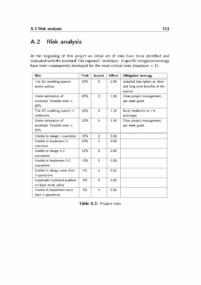
A.2 Risk analysis 113

A.2 Risk analysis

At the beginning of this project an initial set of risks have been identi�ed andevaluated with the standard �risk exposure� technique. A speci�c mitigation strategyhave been consequently developed for the most critical ones (exposure > 1):

Risk Prob Impact E�ect Mitigation strategy

The 3D modeling system

seems useless

50% 5 2.50 Detailed description on short

and long term bene�ts of the

system

Under estimation of

workload. Feasible work <

80%

80% 2 1.60 Close project management,

per week goals

The 3D modeling system is

ine�ective

30% 4 1.20 Early feedbacks on the

prototype

Under estimation of

workload. Feasible work <

50%

20% 5 1.00 Close project management,

per week goals

Unable to design 1 operation 40% 2 0.80

Unable to implement 1

operation

60% 1 0.60

Unable to design 2-3

operations

10% 5 0.50

Unable to implement 2-3

operations

10% 3 0.30

Unable to design more than

3 operations

5% 5 0.25

Unsolvable technical problem

on basic mesh editor

5% 5 0.25

Unable to implement more

than 3 operations

5% 4 0.20

Table A.2: Project risks

114 Project management

Appendix B

Prototype

B.1 The shader

The shader is one of the most complex components of the current prototype andalthough it isn't part of core of this project, it is interesting from both a technicaland a design prospective. The shader has been developed for two speci�c purposes:

Feedback: in order to understand and to feel comfortable with the modeling tool itis important that the user has real time feedback on the mesh structure, suchas information regarding surface curvature, wireframe view, a clear distinctionbetween loops and backbones, feedback on feature distribution along themodel and of course a selection tool to highlight which part of the mesh willbe a�ected in the current operation.

Performances: the traditional OpenGL approach to combine di�erent informationon the same image uses di�erent rendering passes on top of each other.This approach intrinsically leads to a general degradation of the renderingperformances and for mid size meshes it can already represent a problem forthe visualization. On the other hand a customized shader can move to theGPU some of the complexity related to feedback visualization and it can keepa single rendering pass regardless the number of feedback involved.

116 Prototype

The shader itself is therefore a combination of di�erent features:

� Basic di�use shader

� Quad based geometry shader and wireframe

� Color coded information

B.1.1 Basic di�use shader

The light model that has been used is a basic per-fragment di�use shader:

diffuse = fragColor ∗max(0, lightDirection · normal) (B.1)

gl_FragColor = diffuse+ ambient (B.2)

B.1.2 Geometry shader and wireframe

It is well know that the geometry shader can be used to place a wireframe viewon top of a solid shaded mesh but the method described in the OpenGL shadinglanguage cookbook [Wol11], based on the distance between the current fragmentand the nearest edge, is typically applied to triangle based meshes and it becomesvery tricky on quads.

The main reason of this increment of complexity is due to the triangulation per-formed in the geometry shader, that doesn't accept quads neither in input nor inoutput [geo]. The standard workaround uses �strip with adjacency� (so the mesh isrendered as a line strip) to produce a �triangle strip� of two elements for each quadin output, but in this way the fragment shader needs to draw the wireframe onlynear the edges that are on the external side of the original quad.

Although this method is still applicable, a more direct technique has been usedin the prototype, where the wireframe has been rendered as a collection of longand thin additional quads, produced on the �y in the geometry shader. This is avariant of the silhouette method described in a famous blog post of Philip Rideout(http://prideout.net/blog/?p=54) and it provides a more direct control over the�nal result.

B.1 The shader 117

B.1.3 Color coded information

The �nal mesh color is completely procedurally generated and it is independent fromthe input values passed in the color bu�er, which has been used to transfer a setof di�erent information. An �rst interesting aspect is that although the color arraycontains per-vertex data, it has also been used to transfer per-halfedge and per-faceinformation:

� The data regarding a speci�c halfedge is stored in correspondence of the vertexpointed by the halfedge itself.

� The data regarding a speci�c face is replicated and stored in correspondenceof all the 4 vertices that de�ne the face itself.

At this point packing a di�erent number of feedback on the 3 color channels is atrivial task:

Red: in the R �eld it has been stored a numeric ID of the feature that the currentface is part of.

Green: this �eld contains a boolean value to de�ne whether the current edge hasto be marked as a loop edge

Blue: in the blue channel a bit-mask has been used to specify if the current vertex,halfedge and/or face has been selected. As the value is a �oat the �bits� havebeen stored as peak values in correspondence of 0.1, 10 and 100.

The feature IDs have been used to procedurally generate the �nal mesh color, in aprocess designed to optimize readability and to emphasize the di�erences betweenconnected features. To achieve this, the ids have been mapped to a limited setof di�erent colors, equally spaced in hue spectrum, that is limited enough to makeeach color clearly distinguishable, but that is big enough to reduce the probabilityto use the same color for connected features.

118 Prototype

Appendix C

Animation techniques

As brie�y described in the dedicated chapter, animations can be de�ned in severaldi�erent languages, each of them at di�erent level of details. The most commonmethods [ana] to describe complex deformations are:

1. Keyframes

2. Animation scripting languages

3. Goal oriented motion

4. Motion capture

C.1 Keyframes

Keyframes is one of the oldest techniques in the history of computer graphics,originally developed in the Walt Disney studios [BW, Las87]. It is a fairly simplemethod where the designer de�nes the poses (vertices positions) in correspondenceof speci�c time stamps, called keyframes, that the system linearly interpolates inorder to approximate the pose in all the in-between frames.

120 Animation techniques

Despite the obvious limitations of this technique, that requires a considerable amountof work in order to de�ne complex animations, this method is still widely used for alarge set of inorganic animations, especially in its improved form where the strictlylinear interpolation has been replaced by more complex interpolation system, typi-cally controlled by a Bèzier curve.

In �gure C.1 for example, it is shown a simple animation where a cube has beentranslated and rotated in 3DS Max using the keyframes technique. Please note howthe interpolation of the in-between frames can be controlled with the curves on theleft side of the screenshot.

Figure C.1: Keyframe animation in Autodesk 3DS max 2012

C.2 Animation scripting languages

A complete di�erent approach is o�ered by script engines, where the deformationis de�ned using descriptive languages. A typical example of animation scriptingis the Improv System [PG96], developed by Ken Perlin and Athomas Goldberg atthe Media Research Laboratory (New York University), where it is possible to de�ne�real=time behavior=based animated actors� [PG96] using a English-like descriptivelanguage. As shown in �gure C.2, in the Improv system the descriptive code is �rstprocessed by the behavior engine to correctly instruct the internal animation engineto �nally produce the right mesh deformation. An example of this method can besee in �gure C.3, where the neutral face (left) has been deformed with a positivesmile (center) and a negative smile (right).

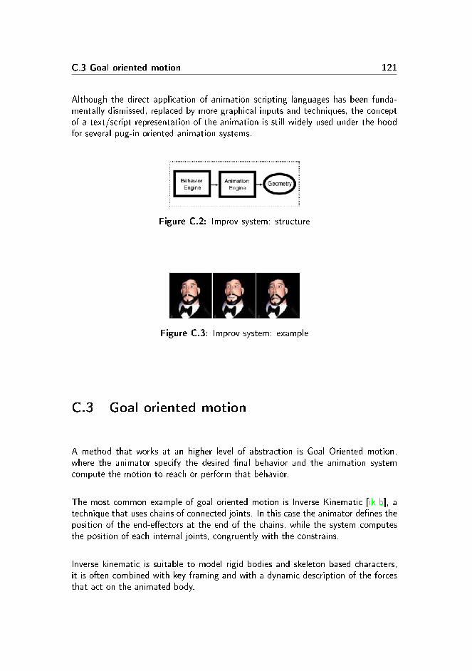
C.3 Goal oriented motion 121

Although the direct application of animation scripting languages has been funda-mentally dismissed, replaced by more graphical inputs and techniques, the conceptof a text/script representation of the animation is still widely used under the hoodfor several pug-in oriented animation systems.

Figure C.2: Improv system: structure

Figure C.3: Improv system: example

C.3 Goal oriented motion

A method that works at an higher level of abstraction is Goal Oriented motion,where the animator specify the desired �nal behavior and the animation systemcompute the motion to reach or perform that behavior.

The most common example of goal oriented motion is Inverse Kinematic [ik-b], atechnique that uses chains of connected joints. In this case the animator de�nes theposition of the end-e�ectors at the end of the chains, while the system computesthe position of each internal joints, congruently with the constrains.

Inverse kinematic is suitable to model rigid bodies and skeleton based characters,it is often combined with key-framing and with a dynamic description of the forcesthat act on the animated body.

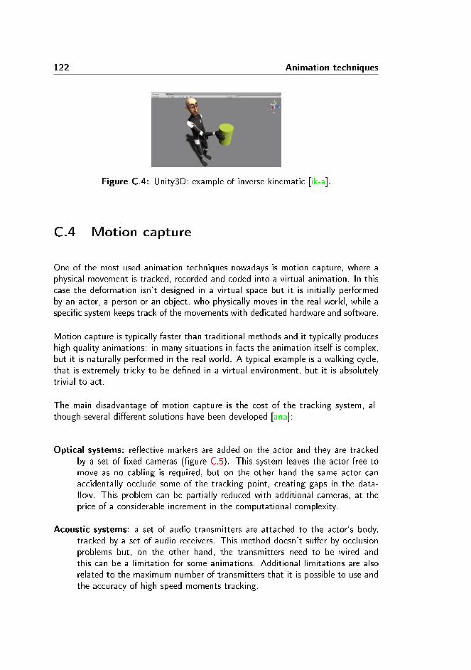
122 Animation techniques

Figure C.4: Unity3D: example of inverse kinematic [ik-a].

C.4 Motion capture

One of the most used animation techniques nowadays is motion capture, where aphysical movement is tracked, recorded and coded into a virtual animation. In thiscase the deformation isn't designed in a virtual space but it is initially performedby an actor, a person or an object, who physically moves in the real world, while aspeci�c system keeps track of the movements with dedicated hardware and software.

Motion capture is typically faster than traditional methods and it typically produceshigh quality animations: in many situations in facts the animation itself is complex,but it is naturally performed in the real world. A typical example is a walking cycle,that is extremely tricky to be de�ned in a virtual environment, but it is absolutelytrivial to act.

The main disadvantage of motion capture is the cost of the tracking system, al-though several di�erent solutions have been developed [ana]:

Optical systems: re�ective markers are added on the actor and they are trackedby a set of �xed cameras (�gure C.5). This system leaves the actor free tomove as no cabling is required, but on the other hand the same actor canaccidentally occlude some of the tracking point, creating gaps in the data-�ow. This problem can be partially reduced with additional cameras, at theprice of a considerable increment in the computational complexity.

Acoustic systems: a set of audio transmitters are attached to the actor's body,tracked by a set of audio receivers. This method doesn't su�er by occlusionproblems but, on the other hand, the transmitters need to be wired andthis can be a limitation for some animations. Additional limitations are alsorelated to the maximum number of transmitters that it is possible to use andthe accuracy of high speed moments tracking.

C.4 Motion capture 123

Magnetic systems: a third approach uses magnetic sensors, strapped on the actor,those are able to calculate �their spatial relationship to a centrally locatedtransmitter� [ana]. Like with acoustic systems, this method requires wiresthat limits the freedom of movement of the actor, and it is a�ected by spaciallimitations, but it doesn't su�er from occlusion problems.

Figure C.5: EUCROMA: example of optical motion capture system(http://eucroma.dk/)

124 Animation techniques

Bibliography

[ana] anand@recoil.org. Animation techniques. http://3d.recoil.org/nojavascript/AnimTech.htm.

[ATC+08] Oscar Kin-Chung Au, Chiew-Lan Tai, Hung-Kuo Chu, Daniel Cohen-Or,and Tong-Yee Lee. Skeleton extraction by mesh contraction. ACM Trans.Graph., 27(3), 2008.

[Bel] Adrian D. Bell. Plant Form. OXFORD UNIVERSITY PRESS.http://www.biodiversitylibrary.org/bibliography/53100.

[BW] N. Burtnyk and M. Wein. Computer-generated key-frame animation.SMPTE, 80(3):149�153.

[Cam] Marcus N Campbell. C++ cubic spline class. https://www.marcusbannerman.co.uk/index.php/home/latestarticles/42-articles/96-cubic-spline-class.html.

[Cas12] Thomas J. Cashman. Beyond catmull-clark: A survey of advances insubdivision surface methods. COMPUTER GRAPHICS forum, 31(1):42�61, 2012.

[CLRS01] T.H. Cormen, C.E. Leiserson, R.L. Rivest, and C. Stein. Introduction ToAlgorithms. MIT Press, 2001.

[Dil] Kernon Dillon. 3d mesh topology tip: Quads vs. trian-gles. http://blendernewbies.blogspot.dk/2008/11/3d-mesh-topology-tip-quads-vs-triangles.html.

126 BIBLIOGRAPHY

[DKM13] Sophie Viseur Dimitri Kudelski and Jean-Luc Mari. Skeleton extraction ofvertex sets lying on arbitrary triangulated 3d meshes. LNCS, (7749):203�2014, 2013.

[Don12] Michael Mc Donnell. Skeleton-based and Interactive 3D Modeling. PhDthesis, Department of Informatics and Mathematical Modelling, Techni-cal University of Denmark, 2012.

[Dra] Nick Dragan. Intro to physically-based deformable body modeling. www.cs.unc.edu/~lin/COMP768-F07/LEC/24a.ppt.

[geo] Opengl wiki: Geometry shader (core v4.3). http://www.opengl.org/wiki/Geometry_Shader.

[GPD] Callum Galbraith, Przemyslaw Prusinkiewicz, and Campbell Davidson.Goal oriented animation of plant development. In 10th Western Com-puter Graphics Symposium, pages 19�32. Citeseer.

[HF01] Jim Highsmith and Martin Fowler. The agile manifesto. Software De-velopment Magazine, 9(8):29�30, 2001.

[Hol06] S. Holzner. Physics For Dummies. Wiley, 2006.

[Hop08] J.E. Hopcroft. Introduction To Automata Theory, Languages, And Com-putation, 3/E. Pearson Education, 2008.

[Hor] Fred Horvat. Atari - jaguar explorer online. http://www.atariarchives.org/cfn/08/09/03/0616.php.

[htt] http://savingyoutime.wordpress.com. C++ matrix inversion(boost::ublas). http://savingyoutime.wordpress.com/2009/09/21/c-matrix-inversion-boostublas/f.

[ik-a] Unity - inverse kinematics. http://docs.unity3d.com/Documentation/Manual/InverseKinematics.html.

[ik-b] Wikipedia: Inverse kinematics. http://en.wikipedia.org/wiki/Inverse_kinematics.

[JAB12] K. Welnicka J. A. Bærentzen, M. K. Misztal. Converting Skeletal Struc-tures to Quad-Dominant Meshes. PhD thesis, Department of Informaticsand Mathematical Modelling, Technical University of Denmark, March2012.

[Jak01] Thomas Jakobsen. Advanced character physics. In Game DevelopersConverence Proceedings, pages 383�401. CMP Media, Inc., 2001.

BIBLIOGRAPHY 127

[JLW10] Zhongping Ji, Ligang Liu, and Yigang Wang. B-mesh: A modelingsystem for base meshes of 3d articulated shapes. Computer GraphicsForum, 29(7):2169�2177, 2010.

[JT05] Doug L. James and Christopher D. Twigg. Skinning mesh animations.ACM Trans. Graph., 24(3):399�407, July 2005.

[jui] Juice it or lose it - a talk by martin jonasson and petri purho. http://www.youtube.com/watch?v=Fy0aCDmgnxg.

[Ket] Lutz Kettner. Cgal user and reference manual, halfedge datastructures. release 4.1. http://www.cgal.org/Manual/latest/doc_html/cgal_manual/HalfedgeDS/Chapter_main.html.

[Kob00] Leif Kobbelt.√3-subdivision. SIGGRAPH '00, pages 103�112, 2000.

[KP07a] Kestutis Karciauskas and Jörg Peters. Surfaces with polar structure.Computing, 79(2-4):309�315, 2007.

[KP07b] Ke�stutis Kar£iauskas and Jörg Peters. Bicubic polar subdivision. ACMTrans. Graph., 26(4), October 2007.

[Las87] John Lasseter. Principles of traditional animation applied to 3d computeranimation. SIGGRAPH Comput. Graph., 21(4):35�44, August 1987.

[LCF00] J. P. Lewis, Matt Cordner, and Nickson Fong. Pose space deformation: auni�ed approach to shape interpolation and skeleton-driven deformation.SIGGRAPH '00, pages 165�172, 2000.

[Lin68] Aristid Lindenmayer. Mathematical models for cellular interaction indevelopment: Parts i and ii. Journal of Theoretical Biology, 18, 1968.

[Lin04] Przemyslaw Prusinkiewicz Aristid Lindenmayer. The Algorithmic Beautyof Plants. The Virtual Laboratory, 2004.

[LLP11] J. Houle L. Leblanc and P. Poulin. Modeling with blocks. Vis. Comput.,(27):555�563, 2011.

[Mot] Giovanni Motta. 3d geometrical transformations - foley and van dam,chapter 5. http://www.cs.brandeis.edu/~cs155/Lecture_07_6.pdf.

[odAtD94] Rieks op den Akker and Hugo ter Doest. Weakly restricted stochasticgrammars. In Proceedings of the 15th conference on Computationallinguistics - Volume 2, COLING '94, pages 929�934, Stroudsburg, PA,USA, 1994. Association for Computational Linguistics.

[PG96] Ken Perlin and Athomas Goldberg. Improv: a system for scripting inter-active actors in virtual worlds. SIGGRAPH '96, pages 205�216, 1996.

128 BIBLIOGRAPHY

[Ros] Rachel Rosmarin. Why gears of war costs $60. http://www.forbes.com/2006/12/19/ps3-xbox360-costs-tech-cx_rr_game06_1219expensivegames.html.

[Roy70] Walker W. Royce. Managing the development of large software systems:concepts and techniques. Proc. IEEE WESTCON, Los Angeles, pages1�9, August 1970. Reprinted in Proceedings of the Ninth InternationalConference on Software Engineering, March 1987, pp. 328�338.

[ski] Ucsd, course 169: Computer animation - skinning. http://graphics.ucsd.edu/courses/cse169_w05/3-Skin.htm.

[So] Da So. Opengl beginning guide(glui). http://soda815.blogspot.dk/2012_08_01_archive.html.

[Sta] Eric Stallsworth. Why are video games so expen-sive? http://www.alteredgamer.com/free-pc-gaming/21118-why-are-video-games-so-expensive/.

[unia] Unity3d: Simple and powerful animation technology. http://unity3d.com/unity/animation/.

[unib] Unity3d: Time manager. http://docs.unity3d.com/Documentation/Components/class-TimeManager.html.

[Wik] Wikipedia. Subdivision surface. http://en.wikipedia.org/wiki/Subdivision_surfaceÂ\protect\T1\textsection.

[WLW07] Jinzhong Wu, Xuehui Liu, and Enhua Wu. Mesh deformation underskeleton-based detail-preservation. In Computer-Aided Design and Com-puter Graphics, 2007 10th IEEE International Conference on, pages 453�456, 2007.

[Wol11] D. Wol�. OpenGL 4.0 Shading Language Cookbook: Over 60 Highly Fo-cused, Practical Recipes to Maximize Your Use of the OpenGL ShadingLanguage ; [quick Answers to Common Problems]. Packt Pub Limited,2011.