a alysis f elast -plastic shell structures
TRANSCRIPT

IV I;L'1 tF3~1
CIVIL ENGINEERING STUDIES
copy3 STRUCTURAL RESEARCH SERIES NO. 324
A ALYSIS F ELAST -PLASTIC SHELL STRUCTURES
Metz Reference ROeJm -; Civil Engineering De~artmen Bl06 C. E. Building University of Illinois Urban&, IllinoiB 61801
by
N. A. SHOEB
and
w. C. SCHNOBRICH
A Report on a Research
Program Carried Out
under
National Science Foundation
Grant No. GK-538
UNIVERSITY OF ILLINOIS
URBANA, ILLINOIS
AUGUST, 1967

ANALYSIS OF ELASTO-PLASTIC SEELL STRUCTURES
by
N. A~ Shoeb
and
w. C. Schnobrich
A Report on a Research
Program Carried Out
under
National Science Foundation
Grant No. GK=538
University of Illinois Urbana, lllinois
August, 1967

ACKNOWLEDGMENT
This report was prepared as a doctoral dissertation by
Mr. N, Af Shoeb. The work was under the supervision of Dre We Co
Schnobrich. The research has been partially supported by the
National Science Foundation under Research Grant NSF~GK 538e
The authors wish to express their thanks to the staff of
the Department of ComputE;!r Sc:;Lence for their cooperation in the use
of the IBM 7094~1401 computer system (supp_orted partially by a - - ,. -- -
gr~nt from the National Science Foundation under Grant NSF-GP 700)0
iii

TABLE OF CONTENTS
ACKNOWLEDGME:NT. LIST OF TABLES. LIST OF FIGURES
...
1. INTRODUCTION ..
1.1. 1.2.
Object and Scope. . Nomenclature, . . .
2. DESCRI~TION OF THE MODEL. .
2.1. 2p 2. 2.3. 2.4. 2.5. 2.6. 2.7.
General . . . . . . . . . . . . Description of the Model. . Coordinate System . . . . . Displacements . . . . . . External Loads. . . . . . . . . . . . Internal Forces ~nd Their Sign Convention . Strain,..Displacement Relations for the Model
Page
iii vi vii
1
1 ,3
5
5 6 7 7 8 8 8
3. RELATIONS IN THE ELASTIC AND PLASTIC PHASES OF THE MATERIAL. 1.3
4~
3.1. 3.2. 3.3. 3.4. 3·5. 3.6. 3·7· 3~ 8.
General . . . . . • . . . . . . q •
Elastic Stress-Strain Relations . Yield Condition ....... . Plastic stress-Strain Relations . Summary of Stress;..Strain Relations.
, Stress,..Displacement Relations. Force,..Displacement Relations, . Equilibrium Eq~ations . . . . . . ...
BOUNDARY CONDITIONS . . . .
4. 1. General.. . • . q ,.
4.2. Simply Supported Edge ...... 0 •••
4.2.1. Node on Edge~ ..... . 4.2.2. Node One-Half Space from Edge . . 4.2.3. Node One Space from Edge. . ...
Free Edg~ . ,. . . . . • . . . . . .'.
4~ 3. i. 4.,3.2. 4.3.3.
Node on Edge. . . .' . .. . . Node One-Half Space from Edge . . . . 0 0 • 0 0
Addi tional Equilibrium Equations for the Free Edge • . . . . . . 0,' • • • 0 • 0 • 0 . '.
iv
13 14 14 15 21 22 23 25
30
30 30
31 32 32
32
33 37
37

v
TABLE OF CONTENTS (cont}d)
4.4. Continuous Edge ...
4.4.1. 4.4.2. 4.4.3.
Node on Edge. 0 0 U U 0
Node One-Half Space from Edge 0
Node One Space from Edgeo
I~RICAL TECHNIQUE
5.l. 5.2. 5.3, 5.4. 5.5.
The Numerical Procedure Initiation of Yielding. Correction Procedure for Plastic Stresses . Solution of the ECluations . 0 • 0 • 0 • •
Coupling of the Two Systems of the Model. 0
6. NUMERICAL RESULTS .. 0 0 •• 0 0 0 0 •
6.1. General Remarks . 0 0 •••••• 0 0
6.2. Cylindrical Shell with Two Edges Simply S'upported and the Remaining Two Free. . . . . . . . 0 • • 0
6 3. Multiple Barrel Shell Simply Supported at Both Ends . 0
7. CONCLUSIONS AND RECO:MJY1ENDATIONS FOR FUTURE STUDY 0
LIST OF REFERENCES
TABLES.
FIGURES ..
APPENDIX A. STRESS-,DISPLACEMENT OPERATORS. 0
APPENDIX B. FORCE-DISPLACEMENT OPERATORS 0 0
Page
40 41 42
43
60
65
68
2

Table
1
2
3
LIST" OF TABLES
Longi tudinal Force N (lb / ft). D
X
Shearing Force N (lb/ft) 0
xy
Transverse Moment M (lb). 0 y
vi
Page
65
66

Figure
1
2
3
4
5a
5b
5c
6a
6b
6c
LIST OF FIGURES
Model Representation of the Shell. . .
A Typical Node . . .
Grid Point Identification and Load Contribution Areas.
Coordinate Axes and Displacements. .
Positive Directions of the Stresses ..
Positive Bending Moments p ••
Positive Twisting Moments ...
Operators for 6ET,6€B • . . . x x T B Operators for 6E ,6E x x T B Operators for 6r AND 6r . . . . xY' xy
. ,
o e' 0
7a Von Mises Yield Surface for a State of Plate Stress. 0
7c
8
9
lOa
lOb
11a
lIb
12a
Yield Locus in Case ~xy = 0
Yield Locus in Case cry ? 0 .
Displacement Points Associated With a Typical Operator ,for Forces and Moments . . . • ,0 • • • • 0 0 0
A Virtual Displacement ou. l' l+ J
The Forces Involved in the Equilibrium Equation in the X~Direction . . ........•.
The Displacements Involved in the Equilibrium Equation in the X~Diiection .... 0 ••••
The Forces and Moments Involved in the Equilibrium Equation in the Y-DireGtion. . .. ....
The Displacements Involved in the Equilibrium Equation in the Y-Direction. • .. ....
The Forces and Moments Involved in the Equilibrium Equation in the W~D'irection. ~ .. .... 0 •
vii
Page
68
68
69
69
70
70
70
71
71
72
73
73
73
75
75
76
77

Figure
12b
13
14
15
17
18
19
20
21a
21b
22
23
24
25
27
viii
LIST OF FIGURES (cont!1
The Displacements Involved in the Equilibrium Equation in the W-Directiono 0 •
Detail of Model at a Free Edge
Equilibrium of a T..,Section at a Free Edge. 0
Junction Geometry and Displacement Configuration of Transversely Continuous Shell. . . . . . .
Modified Junction Geometry of Transversely Continuous Shell at Nodes One-Half Spacing From Valley. 0 0 0 0 0
A General Flow Diagram . 0 • • •
Correction of Plastic Stresses
Coupling of the Two Systems in the Model .
Simply Supported Cylindrical Shell With the Longitudinal Edges Free. . 0 0 0 • 0 • 0 0 0
Progression of Yielding for the Cylindrical Shell With the Free Longitudinal Edges. 0 0 0 0 0 • 0 0 0 0 0 0 0
Final State of Yielding for the Cylindrical Shell Shown in Fig. 20 . . . . 0 • • • • 0 •
Load~Deflection Curve for the Center of the Free Edge and a Point Half a Space From It 0 0 • 0 0 0
The Displacement W' at the Midspan Section of the Cylindrical Shell with the Free Longitudinal Edges 0
The Displacement w Along the Free Edge . 0 •
The Displacement w Along a Line Extending From the Free Edge to the Simply Supported Edge 0 0 • •
Variation of the N Force at Midspan Section in the Cylindrical Shell ~ith Free Longitudinal Edges ..
Variation of the N Force Along the Free Edge" 0 • x
28 Variation of the N Force Along the Simply Supported Edge xy
Page
77
78
78
79
79
80
81
81
82
83
85
86
88
90
91

Figure
29
30
31
ix
LIST OF FIGURES (contYd)
Variation of M at Midspan Section in the Cylindrical Shell With Fre¥ Longitudinal Edges . 0 0 •••• 0 • 0
Comparison of the N Force Distribution at Mid Section as Determined by th~ Model and by Manual 31. . .
Progression of Yielding for a Cylindrical Shell Continuous in the Transverse Direction . 0 0 0 •
32 Load-Deflection Curve for the Node With the Maximum
33
35
39
A-l
A-2
A-3
A-4
A-5
A-6
Deflection . . .
The Displacement w at Midspan Section for the Multiple Barrel Shell.. . 0 • •
The Displacement w Along the Valley.
The Displacement w Along a Line Extending From the Continuous Edge to the Simply Supported Edge 0
Variation of the N Force at Midspan Section in the Multiple Barrel Sh~llo . . . 0 • 0 Q • • • •
Variation of the N Force Along the Valley of the Multiple Barrel Sh~ll. 0 0 0 0 • • • 0 0 • 0 0 0 0
ill I:? €I 0
Variation of the N Force Along the Simply Supported Edge of the Multipt¥ Barrel Shell. . 0 0 0 0 0 0 0 • 0
Variation of the M at Midspan Section in the Multiple Barrel Shell .yo .. 0 •• 0 0 ••• 0 • 0 0 • 0 •
Operator for T a 0
x
Operator for B (J 0
x
Operator for T a y
Operator for B a . 0
y
Operator for T
T xy
Operator for B T xy
Page
93
95
97
99
100
101
102
103
104
106
107
108
109
110
111

x
LIST OF FIGURES (cont!d)
Figure Page
B-1 Operator to be Used With N 113 x
B-2 Operator to be Used With N 114 Y
B-3 Operator to be Used With N 115 xy
B-4 Operator to be Used With M 116 x
B-5 Operator to be Used With M 117 Y
B-6 Operator to be Used With M . 118 xy
1. INTRODUCTION
101. Object and Scope
Beginning with the design of the first shell roof structure(22)*
and continuing to the present day, 'engineers have based their design of
shell structures ,on the classical theory of elasticity. Experience has
shown that employing elas·tic design procedures usually provides struc
ture s that are adequate under service loads. Some engineers -' (1,21,25)
however, prefer ultimate load methods for the design of reinforced
concrete shells. Johansen(2l) for example feels that it is irrational
to solve the shell by a fine mathematical work based on the theory of
elasticity and then sum up the tensile stresses into a tensile force and
determine the reinforcement by dividing this tensile force by the working
stress, ignoring the fact that the deformation and the working stress
do not correspond. He thus suggests·that the working load must be fixed
according to the ultimate load. Limit analysis techniques have also
been inyestigated for shells of homogeneous materials. With a limit
anaiys is, upper and IOvler bound solutions are sought. For the most part
these solutions have only been found for rotationally symmetri.c shells.
The one ~xception to this is the paper by Fialko. (14) He inVestigated
upper and lower bound solutions for a cylindrical shell roof under radial
loading.
There remains a gap in the knowledge of the behavior of shell
structures for the whole region between the elastic limit and the
*. Numbers in. parentheses refer to entries i.n the Li st of References.
1

2
ultimate load. The redistribution of stresses in the shell after
exceeding the elastic limit and the elasto-plastic response are phases
that need closer investigationo
The object of this investigation is to stu,dy the behavior of
a cylindrical shell roof between the end of the elastic stage and the
final ultimate capacity 0 To achieve this purpose a mathematical model
is used to replace the continuum 0 By the use of electronic computers
this model makes it possible to simulate an actual exper:imental test in
the laboratory. The model consists of rigid bars joined together
deformable nodes. The nodes are of the sandwich type and their outer
layers bear the material properties of the shello This model is adapta
ble for any kind of shallow shell rectangular in pIan form but it will
be used here only for cylindrical shells as an example to demonstrate
the applicability of the methodo Different boundary conditions are
formulated for the model. The di.splacements in the model are defined
so that it is pas sible for all for ces to be found at ea ch node 0 fI,lh:is
feature is particularly desirable :in solv.ing an ela,stic c
The material iE) assumed elasti.c perfectly plastic. the
elastic range it ~s assumed to obey Hooke 1 slaw. For the deter:J!in9. tj,on
of the ini,tiation of the plastic flow the Mises-Hencky- cr1.ter i,on
is used. In the plastic range an incremental form of the Prandtl~Reu.ss
relations, modified for-the state of plane stress) is usedo
increasing the load in small ,finite increments it is possible to trace
the progression of yie;:Ld zones in the shell. For each load lncrem,ent
all the displacements) forces, and moments are determi.ned in tb,emod,el c
The load displacement characteristic is thus studi,edo Due te t:t;e

3
complexity of the problem an extensive program for the IBM 7094 computer
is developed to handle all the calculations 0
Two illustrative problems are presented in Chapter 60 The
first is a single barrel cylindrical shell simply supported a+ i,ts ends
and with its longitudinal edges free. The second problem is that of a
multiple barrel shell also simply supported at both ends 0
Since the design objective is to utilize the material fully,
an understanding of the behavior of shell structures is j,nvaluable, as
the usual theory of elasticity does not provi,de an adeC].uate guide 0
However , with an elasto-plastic analysis) small plasti,c strains might
be allowed in an effort to use the material more efficiently 0
1.2. Nomenclature
The symbols used i.n thi,s study are defined when they first
appear. For convenience they are sum.mari,zed below 0
e mean normal strain
e ,e)e ::::: deviatoric strai.n components x y Z
E
G
h
K
L ,L x y
M ,M x Y
modulus of elast:ic~i ty
modulus of rigidity
thickness of shell
the second stress invariant
yield stress in simple shear
bulk modulus E
grid. length in the x and y directi,ons) respectively
moments about the x and y axes, respectively

M xy
N )N x y
N xy
p
R
s
s s s X' y' Z
t
u,v,w
w
E ,E X Y
e
v
CJ a x··' y
'I xy
cp
K ,K x Y
K xy
4
twisting moment
axial forces in the x and y-directions, respectively
i.n plane shearing force
uniform applied load
normal shearing force perpendicular to the y-axi.s
radius of shell
mean normal stress
deviatoric stress components
spacing of layers
displacements in the x, y and z directions, respectively
work performed by stresses during plastic distortion
external loads in the x, y and z dire.ctions, respect i vely
angle between rigid bars in the yz plane
shearing strain
strains in the x and y-directions J respectively
rotation of rigid bars
Poissonu,s ratio
stresses in the x and y-di.rections, respectively
shearing stress
half the openi.ng angle of the shell
curvatures in the x and y-directions) respectively
twisting curvature
2& DESCRIPTION OF THE MODEL
2.10 General
In the analysis of plates) shells} and simIlar complex struc-
tures) the concept of us ing a phys ical analogue lends itself read~i.ly to
the solution of such problems. In the application of the analogue
method the continuous medium of the structure is replaced by a model
which consists of rigid bars joined by deformable nodes 0 The nodes
possess the desired material properties of the med1lli1la Such a model was
used by Schnobrich (34) for the analys1s of cylindrical shells J assum:ing
the material to be elastic. In that model the normal stresses were
defined at one set of points) while the shear stresses were defined at
yet a different set of points 0 Although the model functi.oned very sa ti.s-
factorily in the elastic region) the separation of the extensional
elements from the shear elements renders that particular model incon-
venient for an extension of the study i.nto the plastic range of mater1al
behavior.
Another model) which may be considered a superposit:i.on of
two of the previous models) 'was developed la ter by Mohraz and
Schnobrich.(27) This later model is used in this work because of its
inherent advantageso The most important advantage insofar as this study
is concerned is that the extensional as well as the shear stresses are
found at the same node 0 This makes it convenient to apply a yield
criterion to the nodes.
5
6
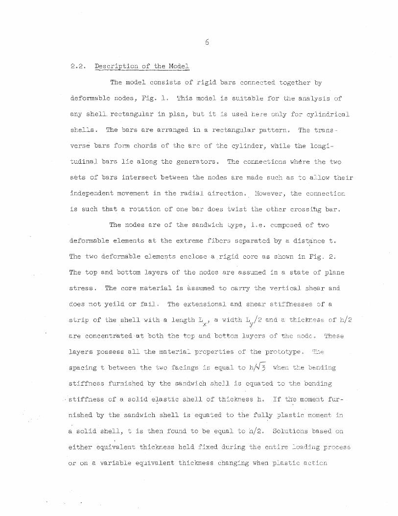
2.2. Description of the Model
The model consists of rigid bars connected together by
deformable nodes) Fig. 10 This model is suitable for the analysis of
any shell. rectangular in plan) but it i,8 used here only for cylindrical
shells 0 The bars are arranged in a rectangular pattern. The trans~
verse bars form chords of the arc of the cylinder J while the longi.=
tudinal bars lie along the generators. The connections wh~re the two
sets of bars intersect between the nodes are made such as to allow theiT
independent movement in the radial direction 0 However) the connecti.on
is such that a rotation of one bar does twist the other cros
The nodes are of the sandvvi.ch type) i 0 e 0 composed of two
deformable elements at the extreme fibers separated by a dis~~nce t.
The two deformable elements enclose a.rigid core as shown in Fig. 2.
The top and bottom layers of the nodes are assu-med i.n a state of plane
stress. The core material is assumed to carry the vertical shear and
does not yeild or failo The extensional and shear stiffnesses of a
.strip of the shell with a length
are concentrated at both the
a width L /2 and a thi.ckness of h/2 y
and bottom. of tIle nodE. 0 iIihese
layers possess all the material propert:ies of the
spacing t between the two facings is equal to h/~3 when t~e
stiffness furnished by the sandwich shell i,8 equated to the bending
. sti.ffness of a solid elastic shell of thickness h. If the moment filr~
nished by the sandwich shell is equated to the fully plastic moment in
a solid shell) t is then found to be equal to h/20 Solutions based on
either equivalent thickness held fixed during the entire process
or on a variable equivalent thickness changing when plastic acticn

7
starts should not differ from each other by any appreci,able amount p
Therefore in this study t is chosen e~ual to hi J3 and is kept constant
throughout both the elastic and plastic phaseso
The system of notation used to identify the different poi,nts
on the model is shown in a plan view i,n Fi,g 0 30 Any node at which the
strains:; stresses) forces) and moments are sought wi,ll always be
designated ij.
2.30 Coordinate System
In the analysis of cylindrical shells it is convenient to use
a moving triad of orthogonal axes as the coordinate system. When the
origin is placed at a deformable node then the x~axis is in the longi
tudinal direction, the y-axis in the direction of the tangent, and the
z-axi.s normal to the tangent 0 Thi,s system of axes is shown i,n Fig. 4
with their positive directions indicatedo
2.4. Displacements
The components of displacement of the shell are defined as
follows (Figso,3 and
a. The displacements are parallel to the x~ax.i.s and are
defined at the intersections of the rigid bars.
bo The displacements are parallel to the y=axis and are
defined at the intersections of the rigid bars 0
c. The IIW It displacements are parallel to the z=ax.is and are
defined at the deformable nodes.

8
2.5. External Loads
Loads applied to the shell are reduced to a number of con-
centrated loads acting at the points where the corresponding displace-
ments are defined. Figure 3 shows the load contribution areas for the
different components of the concentrated loads. One loading of
particular interest in regard to shell roofs is a uniform load acting
vertically downward on the shell. Such a load has two components: one
in the direction of the normal to the shell -direction), and the
other in the tangential direction (y-direction).
2.6. Internal Forces and Their Sign Convention
The positive directions of a~:. a'- and T for both the top x' y' xy
and bottom layers of a node are shown in Fig. 5&0 Also the forces N ) x
N ) and N have the same positive directj,on as the;ir corresponding y xy
stresses. The positive directions for the moments are as shown in
Figs. 5b and 5c.
2.7. Strain-Displacement Relations for the Model
The strains which are required are those of the top and
bott'om layers of a node. These strains are defined in terms of the
displacements of the middle surface. Although there is no deformable
layer at the middle surface it is still convenient to define a pseudo
set of mid-surface strains and curvatures and use them to find the
strains at the top and bottom layers. These pseudo mid-surface strains
and curvatures are established by the geometry of deformation of the
nodes. They are similar to the finite difference form of the strains

9
and curvatures developed about the middle surface of a real continuous
shell. Referring to Fig. 3, the mid-surface extensional and shearing
strains for a typical interior node ij are~(27)
1 (ui +lj u. 1') E -xij L 1- J x
1 (v .. 1 v
ij_1
) 1 (2.1) E yij - - f? w ij
L cos f? 1J+ R cos Y 2 2
I 1
(uij+l u. , 1) 1
(v '+ l ' v. 1') - + -xyij L 1J- L 1, ...LJ 1,- J Y x
The bending and twisting curvatures in terms of the rotation of the
rigid bars are:
1 (8 , l' 8 . '1') K xij L -
x xl,+ J X1-,~J
1 (8 ,. 1 8 'I (2.2) K =
yij L Y1J+ yij-l) Y
K •. XY1J
)
Tihe rotations of the different bars in terms of the displacements are
found to be:
e 1 (w. +2' w .. ) xi+lj L -
x l' J 1J
e 1 (woo w. 2.) xi-lj -L 1J 1- J x
~ L
(203)
e 1 y 1 (itl ij+2 w .. )] f3 v, . 1 + -- -yij+l L _ 1J+ f2 1J
Y cos 2
cos 2
10
1 ~ 1
1 Y - w .. 2)J e
yij-l L (3 vil=l + --(3 (wo 0
y cos _ u cos ~ lJ lJ-2 2
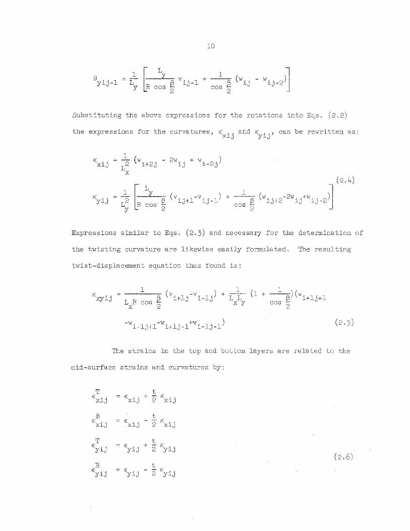
Substituting the above expressions for the rotations into Eqso (202)
the expressions for the curvatures) K '" and K . 0) can be rewritten as~ XlJ ylJ
1 (w", 2' 2w, . w, 2') K,
12 +
xij l+ J lJ l- J' x
(204)
1 ~ L
1 )l y (v 0 , l-v" 0 1 K yij T2 p. + --- -2) I cos' !:::,
lJ+ lJ- cos E .LJ _I Y 2 2
Expressions similar to Eqs. (203) and necessary for the deteTIDination of
the twisting curvature are likewise easily formulated. The resulting
twist-displacement equation thus found is~
K xyij 1 1
~ (v, l'-v o 1') + L L T.lJ R _ l+ J l- J
x cos 2 x Y
-w. 1 0 1" =W" ',1-" l+w 0 'l 0 'l) l~ J+ l'T J- l-, J-,
1 " + --(3)
cos ~ 2
( ~ r\ _,0) )
The strains in the top and bottom layers are related to the
mid-surface strains and curvatures by~
T t E xij E xij + 2
K xij
] t E xij E xi,j 2
K xij
T t E E + - K yij yij 2 yij
( !' 200 ] t
E yij E yij 2 K yij

11
T t Ixyij = I xyij + 2 Kxyij
B I .. = I ..
XYl,J XYl.J t
- - K 2 xyij
Substituting Eqso (2.1)) (2.4)) and (2.5) in the above equations) the
expressions for the top and bottom strains are found to be~
T E .. X1J
B E . , X1J
r]l
E.J.. •• YlJ
B E .. Y1J
T I ..
XY1J
B I " XY1J
1 t 1· (u, l'-u. I') + -2 (w. n.-2w .. +W. 2')
X 1+ J 1- J 21 l+cJ 1J 1- J x
1 ( ) t " _ '1 L u. l' -u, l' - 2 (w. 2' -2w .. +W, 2' J X 1+ J 1- J 21 1+ J 1J 1- J
x
1 (1
+ t Cw,. 2-2w, .+W .. 2) 'J ) ( ')
~ + 2R v .. I-v., 1/ +
212 ~ 1 • 1J+ 1J- 1J+ 1J. ,lJ-:-
y cos
2
1 p.. iif ••
R cos 1:::: 1J 2
cos Y 2 v/
1 t t - 2R ) (v ... I-v. . 1) - 2 f3 (w,. 2 -2w .. +W. . 2)
1J+ 1J - 21' cos _' 1J+ lJ 1.J-1 cos f:? y 2
1 f:? wij
R cos 2
Y 2
1 1 1 (u. "l-u " 1) +
y 1J+ 1J-\
-v, 1') l-_ J
t + 21 L
x y (1 +
1
cos 2
2R cos 2
(w, I' 1-w, I' 1-w, I' 1+ J+ l- J+ l+ J
t 1 1
Y
)" 1 '1 1 - u , . 1 + ~-+ lJ- 2R cos
( ) v, I' -v. I'! l+ J 1- J'
t - 2LL
x:y +--
2
2
(w. l' 1-w . 1" -w .. l' l+W ' l' ,) l+ J+ l- J+~ l+ J- l- J-~

12
where the superscripts T and B stand for the top and bottom layers of
the node, respectively. In the above equations cos ~/2 will be assumed
equal to 1 as ~/2 is small, and it v.TaS found that the final results are
affected only slightly by this approximationo
As the load on the shell is increased progressively the dis
placements increase incrementally. Thus Eqs. (2.1), (2.2),9 and (2.7)
are used in an incremental form, i.e" 6E and 6j{ instead of E and K and
also 6u, 6v, and 6w instead of u, v, and w,
All the above strain displacement relations may be presented
in the form of operators. The operators for the top and bottom strains
(Eq. (2.7) with cos ~/2 = 1) are shown in Figs. 6a, 6b, and 6c.

3. RElATIONS IN THE ElASTIC AND PlASTIC PHASES OF THE :MATERIAL
3010 General
In this study the deformable material of the nodes is assumed
to be elastic-perfectly plastic. To make such an assumption it is
necessary to define three essential aspects of material behavior~
1) The stress-strain relations in the elastic region.
2) A yield criterion that defines the limit of elasticity
under any combination of stresseso
3) The stress-strain relations in the plastic regiono
The stress state at a point of a body when referred to
cartesian coordinates is described mathematically by a stress tensor.
Geometrically thi$ state of stress can be represented by a po:int plotted
in I!stress space 0 II The coordinates of the point are the components of
the stress tensor" and the vector from the ori.gin to the stress poi.nt
is called the stress vector 0 In general, there are nine components of
stress, but considering moment equilibrillID of an element of the material
it follows that the stress tensor is symmetric 0 Thus only six components
of the stress are independent. A change in a state of stress is repre-
sented by a vector from one point in the stress space to another.
In the stress space the mathematical expres-sion defini.ng the
limit of elasticity is represented by a surface which is called the
yield surface 0 This surface encloses a region in which only elasti.c
changes in the strain occur. For a perfectly plastic material the yield

14
surface is fixed in this stress spaceo A stress point cannot be located
outside the surface. When the stress vector reaches a point on the
surface further changes must be associated with movement along or a
return inside the yield surface. Plastic deformation occurs for move-
ments on the yield surface.
3.2. Elastic Stress-Strain Relations
In the elastic region of the materi.al behavior Hooke j slaw
is assumed, thus the stresses are linearly proportional to the strains.
The following relations between the stresses and strai.ns are expres sed
in an incremental form to suit the method of analysis used in thiB study.
For a state of plane stress the incremental stress-strain relations are:
~0 E
(6E + V ~E ) x
l-v 2 x y'
~0 E
(6E + V 6E ) (301) y
l-v 2 Y X
~'r E
!:i,,( xy 2(1+v) xy
To apply these relations to either the top or bottom layer of a node
the corresponding strains should be usedo
3.3. Yield Criterion
The yield criterion is the condition defining the limit of
elasticity under any combination of stresses. It is represented by a
surface in the stress space. The yield criterion which is assumed here
is the Von Mises yield cri teriono It states that plastic flow ,,,,ill

15
2 start if the second stress invariant J2
reaches the value k .' where k
is the yield limit in simple shear. This simple shear yield limit is
expressible as ~
k o
o
~3
where 00
is the yield stress of the material in simple tension. If J2
is less than k2
this means that the point is still elastic.
The yield criterion is applied in this problem to both the
top and bottom layers of each node to check whether or not the specific
layer has yielded.
For a state of plane stress the yield criterion reduces to~
1 (0 2 + 0 2 _ a 0 ) + ~2 3 x y x y xy
The above equation is repres en ted by the surface shov-ln in Fig. 7a when
the coordinate axes are taken to be 0 .' 0 and ~ x y xy
If the surface is
cut by the plane ~ = 0) the relation between 0 and xy x
is represented
by the ellipse shown in Fig. Tb. If the surface is cut by the plane
o = 0-, the relation between 0 and 'I is represented by the ellipse y x xy
shown in Fig. 7c.
3040 Plastic Stress-Strain Relations
In the case of a perfectly plastic material once the stress
vector touches the yield surface plastic flow takes place. During
plastic flow the rate of change of the plastic strain is, at any

16
instant) proportional to the instantaneous stress deviation. This is
known a's the Prandtl-Reuss theory. (19,,20) To present the stress -strain
relations based on that theory it is convenient to first define the
following quantities.
The mean normal stress (when a z
1 ( \ s=- 0 +0) 3 x y
The deviatoric stress components:
s x
s y
The mean normal strain:
e 1 -(E +E +E-) 3 x y z
o - s" y
The deviatoric strain components~
e x
e y E - e" y
o)~
s z
e z
a - s z
E - e z
-s
Only those relations which are of use in the case of plane
stress problems are written below. Also, to suit the numerical
technique used in the analysis" the relations are presented in an in-
cremental form rather than the r,ate form. In their general incremental
form these telations ar~:(20)
6s x
2G(6.e _ 6.W s ) x 2x
2k

.6s Y
( .6W ' 2G 6e - - s )
Y 2k2 y"
where G is the shear modulus~
G E
2(1+V)
17
6W is the incremental form of the rate at which the stresses do work
during plastic flow in connection with the change of shape. In its
general form 6W is equal to~
6W s 6e + s 6e + s 6£; + 'T 61 + 'T 61 + 'T 6; x x y y z z yz yz zx zx xy xy
By its nature 6W is essentially a positive quantity during plastic flow 0
In the case of plane stress problems 'T and 'T are zero and the expres-yz zx
sian reduces to~
6W s 6e + s 6e + s 6e + 'T 6; x x y y z z xy xy
Substituting Eqso (3.4) and 06) into Eqo .8) and then using
Eqs. (3.3) and .5) the expression for 6W is reduced to the following:
6W a 6E: + a 6E + T 61 - 3s6 e x x y y xy xy
but
"6e 6s 3K
where K is the bulk modulus and is equal to~

18
K = E
3(1-2v)
Thus:
6W a 6E + 0 6E + 1" b.y s6s (309) x x y y xy xy -K
If complete incompressihili ty is assumed K tends to 00 and the last tenn
in Eq. (3.9) becomes zero.
To reduce Eqs. (3.7) to the special case of plane stress the
following procedure is adopted. (23) Equations (3.4) are written in
the incremental form and the stresses placed on the left-hand side of
the equation with the following result:
6rJ +.6tJ /;:;a =68 + 6s = 6s +
x Y x x x 3
(3.10) 6a + 60
bn =68 + 6s =68 x "l + y y y 3
Equation (3.9) is substituted in Eqso (307) then the resulting expr~s=
s ions subs ti tuted in Eqs. (3"010) Q Thus, two equations in two unknowns J
6a and 60 ,result. Upon solving these two equations the following x y
expressions for Dc and 60 are obtained. x y
~EX(4 -
2 2 2 0 1" o 0 1"
D.o CA x 4G ...&..) + 6E (2 "'" 2..L 4G ...BL) , ..... -+ x k2 3K '2 Y k
2 3K k2 L k
01" 2G
(0 -0 )
Txyll + 61' . (- ~+ if.. x (3.11) xy' k
2 3K k2
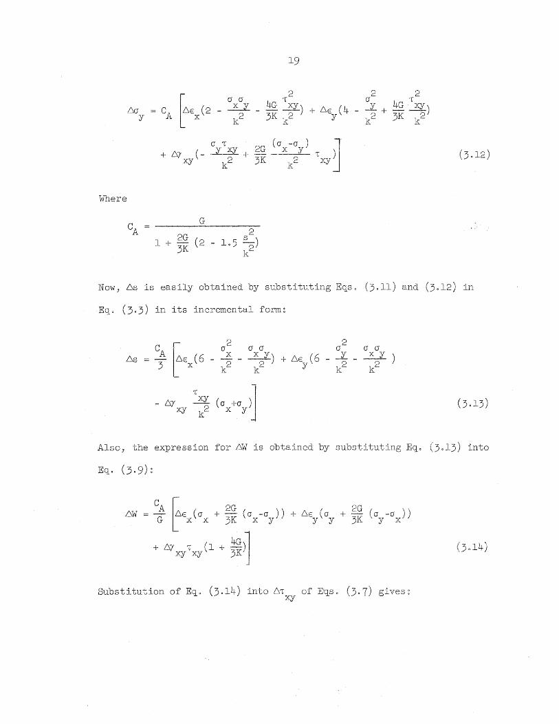
Where
19
2 2 2
[
0 0 4G 1" 0 Y 4G 1" xy 60 = C 6E (2 - ~ - - x
y) + 6E (4 - 2" + 3K 2)
y A x k2 3K k2 Y k k
G 2
1 + 2G (2 - 1.5 S2) 3K k
3.12)
Now, 6s is easily obtained by substituting Eqso .11) and (3012) in
Eqo (3.3) in its incremental form~
CA r 2 2
0 o 0 0 o 0
6s = - 6E (6 - x 2L) + 6E (6 - 1_ ~ 3 x k2 2 ' y k2 k2
k
1" - 6;
xy (0 +0 )J xy k2 x Y
Also, the expression for 6W is obtained by substituting Eqo (3013) i,nto
A ,2G \ C ~ 6W = --G' 6E (0 + --K (0 -0 ))
x x 3 x Y
4G 1 + 6; l' (1 + 3' 'K) xy xy ..
Substitution of Eqo (3.14) into 61" of Eqso (3.7) gives~ xy
3014)

20
,- a 'L 2G (ay-ax )
6'L 6E (__ x xy ) xy CA _ x k2 + 3K k2 1;xy
a 'L (a ~a ) + 6E (_ ~~~ .+ 2G x Y T )
Y k2 ' 3K k2 xy
2 2
+ b:Y (1 _ Tz:y_ + 4G (1 _ Tz:y __ 0.75 S~))l xy k2 3K k2 k .J
When 6a ) 60 ) 6'L J 6s) or 6W are used for either the top or bottom x y xy
layer of a node the correspondi.ng top or bottom strains and stresses
are used in their corresponding equationsQ
For complete incompressibility K ~ 00 J and Eqs Q (3011)) (3·12) J
(3. 15)) (3.13) J and (3.14) simplify to the following form:
= GrEx (4
2 (-T 0 lj a cr a
oa x + OE (2 Y x' xy x
k2 - ---) +
k2 x Y k
2
GrEx (2 2
~'T~~~l1 a a cr
oa _l_l:..) .-\-- 6E (4 _L) + y k
2 y' 21 k
2 2 d a a a a cr
x x y\ + 6E (6 2- x y. - ~2-j - -) k
2 Y k2 2 .
k k
T
+ 6/ ...7:J!.. (0 +0 ~ xy
k2 x Y
oW cr OE + cr oE + 0"1 x x Y Y xy 'xy

21
305. Summary of Stress~Strain Relations
The stress-strain relations in their incremental form may be
represented for both the top and bottom layers of a node in the
following form~
6,0 Cll 6,Ex + C12 6,E + C13 6,)'xy x Y
6,0 C21
6,E + C22
6,E + C23 6,)' xy (30 y x y
m C31
6,E + C32
6,E + C33
ti'/ xy x y xy
Where in the elastic range the coefficients C for both the top and
bottom layers are~
Cll C22
E
I-v 2
C12
~ I-v
2 (3017a )
C13
C23
0
C33
E 2(1+v)
and in the plastic range~
CAr 2
~~ ~~ 2
J 0
, Cll x
- - + k
2
't
CAt 2 -
crcr 4G~ 1 C12
-~--~ k2 3K k2
CAt o a
2G (0 -0 ')
~XYJ C13
~+ y.. X$
2 ' 3K k2
k (3017b)

22
CA[4 2 2-
a 4G Txy J C22
~+ k
2 3K k2
CAt a T
2G (a -a )
TxyJ C23
yxy + x y
k2 3K k
2
C33
where
2 '1."
4G (1 c 1 ~+ A
k2 3K
G 2
1 + 2G (2 _ 1 5 s )' 3K .. 2"
k
2
2J T
_ -BL s '
k2 - 0075 k2 )
It should be noticed that in the elastic range the coef-
ficients C are constants. Also they are equal for the top and bottom
layers 0 However, in the plastic range they are no longer constants
as they depend on the stress level. Furthermore, they are no longer
equal for the top and bottom layers as the top and bottom stresses)
in general, are different.
3.6. Stress-Displacement Relations
In Section 2 .. 7 the strain-displacement relations were obtai.ned
and in Section 3.5 the stress-strain relations were presented in their
most general form. By combining both these sets of equaticns the
stress-displacement relations result. The six stresses in terms of
their displacements are best shown in the form of operators 0 These
operators are listed in Appendix Ao

23
3.7. Force~Displacement Relations
The stresses in the upper and lower facings of the nodes are
assumed to be uniformly distributed over the thickness of the facingq.
Thus the following relations, in their incremental form" for both top
and bottom facings are~
6,NB xy
L h T ~6a
4 x
L h B .2- 61:
4 xy
Instead of the above equations the forces and moments can be
expressed in a manner similar to the finite difference form developed
about the middle surface of a real continuous shell. Then the following
expressions are defined:
~ x
6M x
~T + ~B x x
A typical operator for any of the above forces involves the displace-
ments shown in Fig. 8. The operators of all the above equations are
shown diagramatically in Appendix B. If Eqs. (3.17) are substituted in I
Eqs. (3.19) the forces and moments are obtained as a function of the
top and bottom strains. To illustrate the form of these relations the
force N is written below~ x
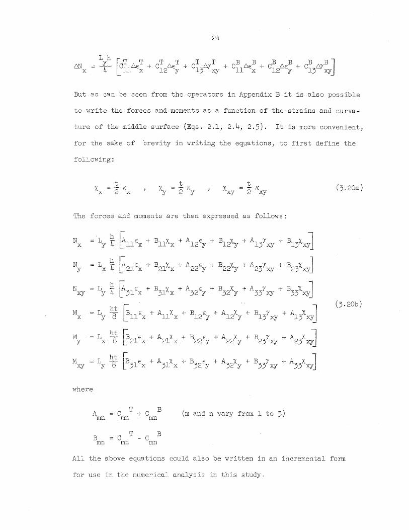
24
But as can be seen from the operators in Appendix B it is also possible
to wri.te the forces and moments as a function of the strains and curva-
ture of the middle surface (Eqso 201, 204, 205)0 It is more convenient,
for the sake of brevi.ty i.n wri.ting the equations) to first define the
following~
The
N x
N y
N xy
M x
M. y
M xy
t Xx :=. - K 2 x
t - K 2 xy
forces and moments are then expressed as follows ~
:= 1 h ~llEX B11Xx + A12Ey + B12X-y + A13! xy + B13x-xyl y 4
::= 1 h ~21Ex B21Xx + A22Ey B22Xy + A23Yxy B23XXY] 1+ + + + x
= 1 h ~31 Ex + B31Xx + A32E + B32Xy + A33,xy + B33xxyJ y 1+ . Y
ht ~llEX A13XxyJ = 1 8 + AllXx + B12
Ey + A12Xy + B I + y 13 xy
= 1 ht ~21E + A21Xx + B22Ey + A22Xy + B23Yxy + A23XJ x ~8 l,... x
= 1 ht
r31EX + A31Xx + B32Ey + A32Xy + B33,xy + A33xxyJ y 8
where
A mn
B mn
C mn
C mn
T
T
+ C mn
C mn
B and n vary from 1 to 3)
B
(3. 20b)
All the above equations could also be written in an incremental form
for use in the numerical analysis in this study,

2.5
.3080 Equilibrium Equa ti.ons
The equ:Lli.briu.rn equa ti.ons for the model are best formula ted
the principle of virtual work. This principle states that for a
system i.n equilibri.um the tctal work done by both internal and external
forces is equal to zero for any arbitrary virtual displacements. This
principle is valid regardless of the material propertieso
If for a vi.rtual displacement the internal work is equal
to I J and the external work done is W v J then ~
I + WI = 0 (3021)
The i.nternal work I is equal to the nega ti ve of the product of the
internal forces times the di.splacements plus the product of the moments
times the rotat ions whi.ch result from the given virtual displacement:
- )' N bd <=
L-J
.For conven1ence :tn fi.nding the di.splacements and the rotati.ons J the
above can also be written as:
TAThere bE: and bK represent the strai.ns and curvatures due to the
vi.rtual di.splacement 0
To generate the equilibrium equation in the x-direction
joint i+lj is given a virtual displacement bU, l' while all the other l+ J
displacement p01nts are restrai.ned from movement 0 As can be seen from
.Fig 0 9 nodes ij and i+2j 11'/111 undergo extensional stra1ns while nodes

26
i+lj+l and i+lj-l will be subjected to shearing strains. Because the
curvature of the shell is zero in the x-direction no rotation results
from the virtual displacement. For a virtual displacement in the
axial direction the internal work is:
I ~ , ,OE " + N , 2,OE . 2 ~ L LXlJ XlJ Xl+ J Xl+ jJ X
- r; , l' lOY , l' 1 + N '1' 10)' '1' 11 L L~YXl+ J+ XYl+ J+ YXl+ J - XYl+ J - _ Y
From Eqs 0 (2.1)
OE " XlJ 1 L- ou, l' l+ J
x
OE , 2' Xl+ J
5)' '1' 1 XYl+ J-,
5)' , l' 1 XYl+ J+
-1 L- ou, l' l+ J
x
1 LOu, l' Y l+ J
-1 L-, ou, I'
l+' J Y
The external work done by the load X. " applied to the point i+lj is ~ l+lJ
W'= X, l' ou. l' l+ J l+ J
Substituting Eqs. (3.24) into Eq. (3.23) and adding the resulting expres-
sion to Eq. (3.25)) the equilibrium equation in the x-direction is
obtained in terms of the forces~
N'2,-N,,+N 'l'l-N 'l'l+X'l' Xl+ J XlJ YXl+ J+ YXl+ J- l+ J o
Similarly for the equilibrium equation in the y-direction joint ij+l is
given a virtual displacement OV, , 1 lJ+
The internal work will be:

27
- M , , OK , . + M . . OK , , L E -
XYl-lj+.l XYl-1J+l XYH1J+l XYH1J+J . X
From the strain-displacement Eqs. (2.1), (2.4), and (2.5) the incre-
mental strains resulting from the virtual displacement are as follows~
OE .. YlJ
OK ,. YlJ
OK .. XYlJ
1 OV, , 1
L cos f? lJ+ Y 2
-1 ov .. 1 L R cos f? lJ+
Y 2
1
f3 OYij+l L R cos -
x 2
The external work will be:
1 -
W = y, . lOv .. 1 lJ+. lJ+
(3.28)
Substituting Eqso (3.28) i.nto Eqs. (3.27) and adding the result to
Eqo (3.29), the equilibrium equation in the y-direction is obtainede
1 f3 (N .. 2 - N .. ) + 1 f3 (M " . - M .. 2) + N . l' 1 ' YlJ+ YlJ R _ YlJ YlJ+ XYl+ J+ cos 2 cos 2
1 Nxyi_lj+l + R ~ (MXYi-lj+l - Mxyi+lj+l) + Yij+l
cos 2 o

28
The equilibrium equation in the radial direction is similarly
formulated by giving the node ij a virtual displacement 6w. ,. The lJ
resulting equation is:
1 L
x (M . 2' - 2M " + M . 2') + Xl+ J XlJ Xl- J L
Y
1 Q (MYij +2 - 2MYij + Myij _2 )
cos 2
L 1 1 + y t3 (N ,,) + (1 + --p,) L (M '1' 1 - M , l' 1
R cos 2" YlJ cos ~ Y Xyl+ J+ xyl:- J+
-M 'l'l+M 'l'l)+Z" xyl+ J- Xyl- J- lJ o
The above equilibrium equations are written in terms of the
forces and moments. By using the relations previously obtained between
the forces and moments, and the displacements) the equilibrium equations
are. expressed in terms of the various displacements. The forces and
displacements involved in the x) y, and z equations are shown diagram-
atically in Figs. lOa) lOb, lla, llb, and l2a, l2b) respectively.
The term cos t3/2 i.s assumed equal to one as was mentioned in
Section 2.7. Also it should be noted that the equilibrium equations
are used in an incremental form as the load i.s progressively increased.
For each load increment 6p the equilibrium equations are formulated for
all the grid points of the model. A set of linear !3.lgebraic simul-
taneous equations result in terms of the unknown increments in displace-
ments Uu, 6v, and 6w. S0lving these equations the increments in
displacements are obtained. Once 6u) 6v, and 6w are known the increments
in the strains, stresses, forces) and moments are easily obtained
throughout the shell. By adding the increments of displacements, strai.ns,

29
stresses) forces) and moments to the values previously obtained the
final values are obtained for each stage of loading. The numerical
technique is described ~n more detail in Chapter 5.

4. BOUNDARY CONDITIONS
4.1. General
The model used in this investigation is adaptable to a
vari.ety of boundary conditions. Of these) the three which are pertinent
to this study are presented below 0 The boundari.es considered include a
simply-supported edge; a free edge; and a continuous edge.
As shown in Section 3.8) the internal work done due to a
virtual displacement can be expressed in terms of strains and curva-
tures (Eq. 3022). For both geometric and forc,eboqpdary conditions the
d.esired representation of the boundary is established by using the
appropriate strains and curvatures for those points close to or the
boundary. Hence the only modification needed for the introducti.on of a
boundary edge is on the strains and curvatures existi.ng thereo
4020 Simply-Supported Edge
The simpJ,.y-supported edge represents the case where the shell
is supported by a diaphragm which is infinitely stiff in i.ts own plane)
but has no resistance to loads normal to its plane 0 Assuming the
simply-supported edge to be parallel to the y-axis the following con~
ditions must be satisfied along that edge~
v
N x
0, w ° OJ M - 0
x
The special strain and curvature relations for points on or near the
30

31
boundary are derived; taking into consideration these specified stress
and displacement values 0
4.2010 Node on Edge
For a node ij on the edge; substitution of Eqo (401) in the
strain-displacement Eqso (2.1) and (204) determines the strain and
curvature directed along the edge. These are~
E " Y1J
o and K .• Yl.J
o
In the Nx and Mx express ions of Eqs" (3020) Al .3
., B13
,,' and Bll B.re equal
to zero in the elastic range 0 When Eqso (402) are used; and Eyij and
, \ K .• are substituted into the Nand M expressions of Eqso (3,,20); YlJ X x
the strai.n and curvature in the x-directions beco:me ~
E •• o and K .. o Xl.J XlJ
In the plastic range the coefficients A13
" B13
;.and Bll can be shm{n to
remain equal to zero for a node on the edge. Thus the above Eqo (4"
is valid in both the elastic and plastic ranges 0
The shearing strain and twisting curvature are obtained by
Since the node represents the material extendi.ng one·-half spacing i.n
froID the edge; Lx/2 i p used in place of Lxo The- appropriate strain and
twist rela tj,ons thu~ become ~
1 2 1. .. = L (D. .. l-u .. 1) + L' (-v. 1')
XY1J y 1J+ 1.J - X 1-. J
K " XY1J
2 ( ) 2 I 2 ". 2 ) LR -v'l"'+L-L \,-w· 1IIl
l '1+w, 1'1' . 1-. J . 1- J+ 1= J-x x Y

32
40202. ~ode One-Half Space From Edge
The expressions for E "J E . oj and K " at a node ij one-XlJ YlJ YlJ
half space interval from the edge are the same as those of an interior
node 0 Since v and ware zero on the edge) the remaini.ng strai.n
expressions are~
K " XlJ
)' ,. XYl.J
1 2 (-3w. . + w. 2') L lJ l= J x
1 L
Y (u. '. 1 - u .. '1) lJ-i- 1.J -. '
1 ( ) 2 ( ) L R -vi _lj ' + 11 -w i .-lj+l + wi - lj - l
x x Y
4.2030 Node One Space From Edge
All strain and curvature quantities for a node i.j one space
from the edge are the same as a typi.cal inter ior node except the expl'es·=
sion for the curvature in the x=direction which becomes~
K .. XlJ
If the edge parallel to the x,...axis J., i 0 eo the longi.tudinal
edge~ is free then the following conditions. must be satisfied along that
edge ~
N o y
N o yx
M o y
R o y

where
and
R Y
21M --L dY
33
Some modifica ti.on in the mqdel is needed along the free edge
to make it possible to define the reaction R at all points along the y
edge 0 This modification requires additional displacements., 5! s J along
the free edge 0 These new displacements are defi.ned at the :intersect:ion
of the rigid bars and are in the radial direction. To account for the
extra unknowns additional equations of equilibri.um along the edge are
developed. These are discussed in Section 4.3.3. The d.etails of the
free edge with the necessary modifications are shown i.n Fi.g 0 130 This
detail was first developed by Mohraz and Schnobrich.
4.3.10 Node on Edge
Due to the Kirchhoff-Love assumption of the preservation of
normals in the classical theory of plates and shells, the condition that
the twisting moment M along the free edge be equal to zero cannot be yx
enforced.. Instead, the reaction R is taken equal to zero 0 If this Y
assumption is 'not used and the shear deformation is taken into account]
the five stress resultants N , M ,N ,M ,and N can be equated to y y yx yx yz
(16) zero along the free edgeo . In this case, the coefficients A31' B31'
A32' B32' and B33 in the Nyx and Myx expressions of Eqsa (3.20) would be
equal to zero in both the elastic and plasti.c ranges a Si.nce Nand M yx yx
would 'be equal to zero), and X would also be found equal to zero a yx yx

34
In this study, however, the classical Kirchhoff-Love hypothes:ts
is assumed to be valid) which means that shear deformation is neglected.
All the coefficients in the Prandtl-Reuss relations are derived in
accord with this assumption. Thus, when A31 ) B31' A32' B.32J and B33
in E~s. (3020) are calculated they are found to be not equal to zero in
the plastic range. The result is that N . which was zero i.n the yx/
elastic range) acquires some small value in the plastic range even when
Y is set to zero. yx
To obtain the twisting curvature K " at the node ij on the XYlJ
edge the rotations of the bars around that node, Fig. 13, need to be
computed first 0 The rotations about the x-axis of the ri.gid bars
(i+lj -1, i+lj) and (i-lj -1) i.-lj) are as follows ~
e " l' Yl+ J
e . 1 Yl- j
L Y ')
+ 2R v i +lj '
The rotati6n about the y-axis of bar (i-lj-l, i+lj-l)
e ,. XlJ Ll (W,.- l . 1 - w. l' 1) .l.+ -J - l- J-x
l'r-< 0
00
14 ") " .013
The rotations about the y-axis of the two auxi.liary bars (i-l, ij) and
(ij J i+1j) are ~
e~. 1 (w, . °i_lj) lJ L lJ X
e~. 1 (Oi+lj w. ,)
1.J L lJ X

35
thus the average rotation at the node ij is~
e " - 12 (e~. + e~,) = 11 (5"1' - 5. I') XlJ . lJ lJ X l+ J l-, J
The twisting curvature is~
K ,,- 11 ( e , l' - e . 1.) + 1 I; 2' (eXl' J' - e ., 1 ) XYlJ . Yl+. J yl.- J' XlJ-X Y
Substituting the values of e in Eqs~ (4012) through (4015) i.nto
Eqo (4016) the twisting curvature is obtai.ned~
1 2 K (v - V ,) + -~ (-2w + 2w ) ., - LxR 'i+1J' i-lJ'; L L . i+1j-l i-lj-l' XYlJ x y
4 +~
x y ( 5 . +1' - 5. 1')
l . J l- J
To obtain the extensional and bending strains E and X at yy
the edge, N , M , and yare set to zero in Eqs. (3.20) in their y y xy
incremental form. Solving these two simu~taneous equations provides
6E and tsx, ) in terms of 6E , 6X '. and. b:.X y y . x x xy
where
6X Y
-0: 6E 1 x (4018)
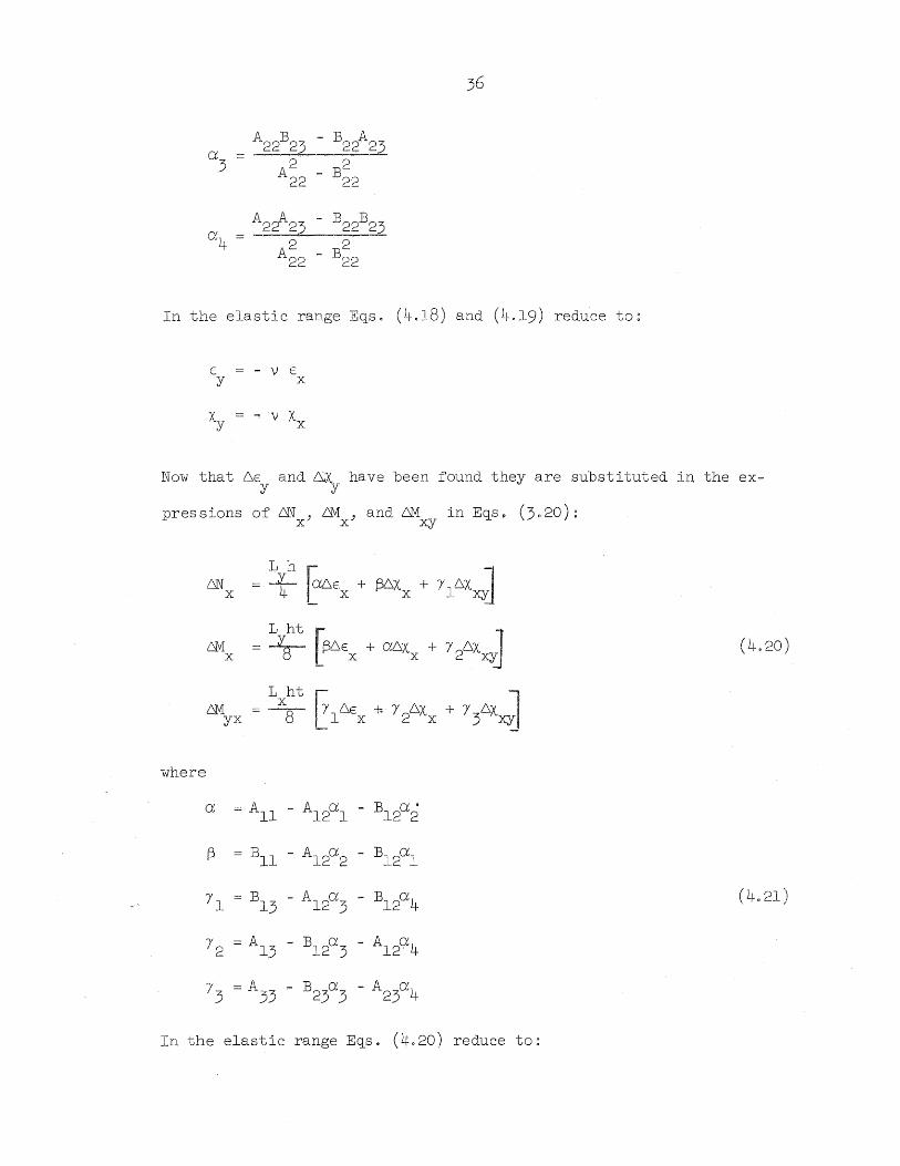
In the elastic range Eqso (4.18) and (4.19) reduce to~
EVE Y X
Now that 6E and ~X have been found they are substituted in the ex-y y
pressions of 6N ) 6M J and 6M in Eqs. (3020): x x xy
(4.20)
L ht fl6Ex -I< Y 3L'iXxJ 2M x
126Xx + yx =-8-
where
CX = All - A12CXl
- B12CX2
f3 = Bll - A12CX2 - B12CXl
11 = B13 - A12CX3
- B12
CX4
(4021)
12 = A13 - B12CX3
- A12
cx4
13 = A33 - B23
cx3
- A23
cx4
In the elastic range Eqs. (4.20) reduce to~
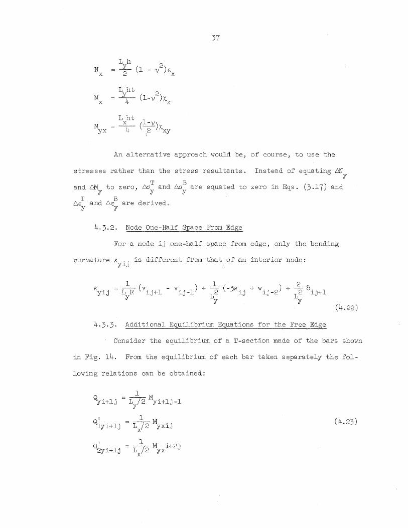
37
L h 2
N = .L.- (1 - v ) E X 2 ' x
L ht ( 2\ M Y
.t _ -4- I-v )X x x
L ht (l-V) M
x yx -4- 2 Xxy
An alternative approach would be) of course) to use the
stresses rather than the stress resultants. Instead of equating 6N y
and L1VI to zero) 6I;T and 6aB are equated to
y y Y zero in Eqs. (3.17) and
T 6E and
B 6E are derived.
Y Y
4.3.2. Node One-Half Space From Edge
For a node ij one-half space from edge) only the bending
curva ture K " i.s d,ifferent from that of an i.nterior node ~ YlJ
(4.22)
4.3.3. Additional Equilibrium Equations for the Free Edge
Consider the equilibrium of a T-sect,ion made of the bars shown
in Fig. 14. From the equilibrium of each bar taken separately the fol-
lowing relations can be obtained~
1 Qyi+lj = ~Myi+lj-l
y
v 1 Qlyi+lj = ~ Myxij
x
Q l 1 M '2' . 1 = r;--rn2 yx l + J 2Yl+. j J.J-.rl C.
X

where
(4024)
For e~uilibrium in the vertical direction~
Q'l' J' +1 + Q2' " 1 - Ql! •• 1 0 Y YlJ+' YlJ+ (4.25)
Combining E~so (4.23)) (4.24) and (4.25) the additional equilibrium
equation at the free edge can be written as~
o (4.26)
4040 Continuous Edge
For a shell that is continuous in the transverse direction
and syrr@etrically loaded) the edge conditions at the junction between
two successive interior shells are~
the horizontal displacement normal to the junction) v 0
the rotation in the transverse direction, e 0 y
39
the shearing force) N 0 xy
the vertical reaction 0
The second condition) that of e being zero, does not remain valid once y
plastic action takes place along the conti.nuous edge 0 It is replaced
by the condition of symmetry of the deflections on both sides of the
continuous edge.
Due to the sharp break in curvature at the junction between
the two shells some modifications are necessary in the nodes along the
edge. The top and bottom layers of such nodes are placed in the hori-
zontal directi.ono The detail of one of these boundary nodes and the
bars connected to it is shown in Fig. 15. From this figure it is noted
that the spacing between the two layers of the node becomes equal to
t In the equations that follow cos ~/2 is approximated
cos B/2 cos Y
by being considered equal to unity, so the spacing is taken as cos y
t
Also shown in Fig. 15 is the geometry of displacements at that particular
node. Nodes which are one-half spacing on either side of the junction
between the two shells are joined together by a horizontal bar as shown
in Fig. 16. This manner of connecting the nodes is in agreement with
the boundary conditions as described above and i.s found to yi.eld good
correlation between the two systems of nodes as explained in Section 5.5.
\tIThen the number of spacings increases in the transverse directi.on, then
in the limit these two nodes joined by the horizontal bar will be almost
like one of those nodes on the junction between the two shells.
The strains and curvatures for the nodes on or close to the
continuous edge are as described below.

40
4Q4.10 Node on Edge
For a node ij on the boundary between the two shells, the
extensional strain Eo. and the bending curvature K 00 remain the same XlJ XlJ
as those of a typical interior node 0 It need only be noted that to get
the strains at the top and bottom layers of a node due to bending K 0 0
XlJ
is multiplied by 2 t
cos t
instead of the usual -20 I
DeLe to symmetry about
the boundary line between the two bays, the sheari.ng strain y 0 0 and XYlJ
the twisting curvature K 00 are equal to zero along the edge~ XYlJ
I xyij 0
K xyij 0
Referring to Fig. 15, the extensional strain in the y .... direction i.s~
E 00
Yl.J 1
1 cos'V (v.. 1 - v. . 1) + y I lJ+ lJ-
2w. 0 tan j 1.J
1 y
Because of symmetry v 0 • 1 lJ+'
-v .. 1 thus: lJ=.
Eo. YlJ
1 -1---'11 (-2v .. 1) + cos I lJ-
Y
2w. 0 tan I' lJ
1 y
(4.28)
The rotation of the rigid bar joining the two nodes ij-2 and ij is:
e 00 1 YlJ-
1 1
Y
The curvature in the y-direction is~
1 K 00 1 (8 00 1 - 8 .. 1) YlJ y YlJ+ YlJ-

41
From symmetry considerations 8 yij+l
-8 thus~ yij-l
K " YlJ
1 L
Y (-28 " 1)
YlJ-
Using Eqo (4.34) the following expression for the curvature K " YlJ
results~
K ,. Yl.J ~
2W' . ~+2w ...I.... " 2 I cos f lJ-
2v,. 1 (tan / - tan f3/2~ lJ- J
4.4.2. Node One-Half Space from Edge
For a node i.j one-half space from the continuous edge) the
strai.ns E ,,) .,. and the curvature K " remain as those of a XlJ xyij) X1J
typical interior node. New expressions must be found for the remaining
strain quantities. Referring to Fig. 16, the extensional strain in
the y-direction is~
1 w. , tan f
( -v. . 1-) + - lJ L a lJ- y
(40}1) E •. Y1J L cos f
y a
For the curvature in the y-direction) both 8 . "1 and v1.J . ...I....1 are set to
Y1J'T ,
zero, then~
K Y
1 ~ -w ij + w.. 2 + v, . 1 (tan fa - tan f3/ 2j T 2 'Y cos I lJ - lJ-.L!y cos 'a a (4.32)
For the twisting curvature K .. , the rotations 8 . l' and 8 .. J . have XYlJ Yl+ J yl.~ -J
expressions similar to those in Eq. (4.34). K " is therefore equal to: XY1J .

K " XYlJ
42
- LIL ~(tanf - tan f3/2) (v, l'-v, 1') l+ J l- J x y
+ cos2 ~ Cw, I' l-w, l' 1) + 2(-w, l' l+w, l' 1)1
I l+ J+ l- J+ l+ J- l- J-
(4.33)
As in Section 4.4.1) to get the strains resulting from the curvatures
at the top and bottom layers of a node the curvatures are multiplied
by t instead of t/2. 2 cos fa
404.3. Node One Space From Edge
For a node ij one space from the edge) the expressions for
the curvatures K .. and K ., must be modified. All the other strains ylJ XYlJ
and the remaining curvature in the x-direction are like those of a
typical interior node. The rotation e needed to get the curvature yij+l
in the y-di.rection has an expression similar to the one in Eq. (4.34).
Thus K " becomes: YlJ
1 ~ij+2 K . . 2 - 2w. , + w.. 2 - v, . 1 (tan f - tan f3 /2) YlJ L cos f lJ lJ- lJ+
Y
The modified twisting curvature is:
5. NUMERICAL TECHNIQUE
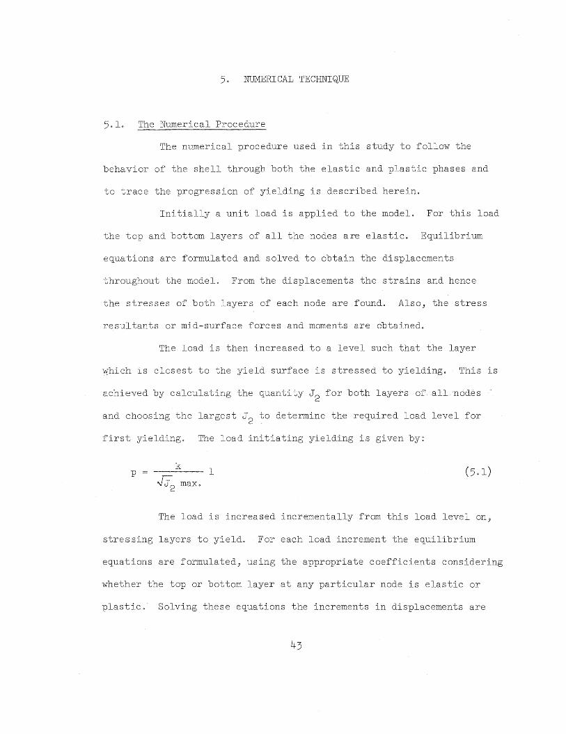
5.1. The Numerical Procedure
The numerical procedure used in this study to follow the
behavior of the shell through both the elastic and plastic phases and
to trace the progression of yielding is described herein.
Initially a unit load is applied to the model. For this load
the top and bottom layers of all the nodes are elastic. Equilibrium
equations are formulated and solved to obtain the displacements
throughout the model. From the displacements the strains and hence
the stresses of both layers of each node are found. Also, the stress
resultants or mid-surface forces and moments are obtained.
The load is then increased to a level such that the layer
Which is closest to the yield surface is stressed to yielding. This is
achieved by calculating the quantity J2
for both layers of all nodes
and choosing the largest J2
to determine the required load level for
first yielding. The load initiating yielding is given by:
k 1 p
JJ; max.
Irhe load is increased incrementally from this load level on,
stressing layers to yield. For each load increment the equilibrium
equations are formulated, using the appropriate coefficients considering
whether the top or bottom layer at any particular node is elastic or
plastic. Solving these equations the increments in displacements are
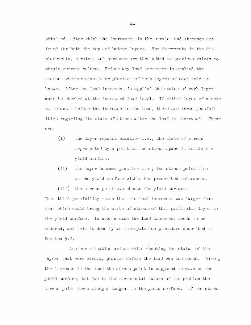
44
obtained) after which the increments in the strains and stresses are
found for both the top and bottom layers. The increments in the dis-
placements) strains, and stresses are then added to previous values to
obtain current values. Before any load increment is applied the
status--whether elastic or plastic--of both layers of each node is
known 0 After the load increment is applied the status of each layer
must be checked at the increased load level 0 If either layer of a node
was elastic before the increase in the load) there are three possibil~
i.ties regarding its state of stress after the load is increasedo These
are~
(i) the layer re~ains elastic--i.eo) the state of stress
represented by a point in the stress space is inside the
yield surface.
(ii) the layer becomes plastic--ioe.) the stress point lies
on the yield surface within the prescribed tolerances 0
(iii) the stress point overshoots th~ yield surface.
This third possibility means that the load increment was larger than
that which would bring the state of stress· of that particular layer to
the yield surface 0 In such a case the load increment needs to be
reduced) and this is done by an interpolation procedure described in
Section 5.2.
e
Another situation arises while checking the status of the
layers that were already plastic before the load was increased. During
the increase in the load the stress point is supposed to move on the
yield surface) but due to the incremental nature of the problem the
stress point moves along a tangent to the yield surface. If the stress
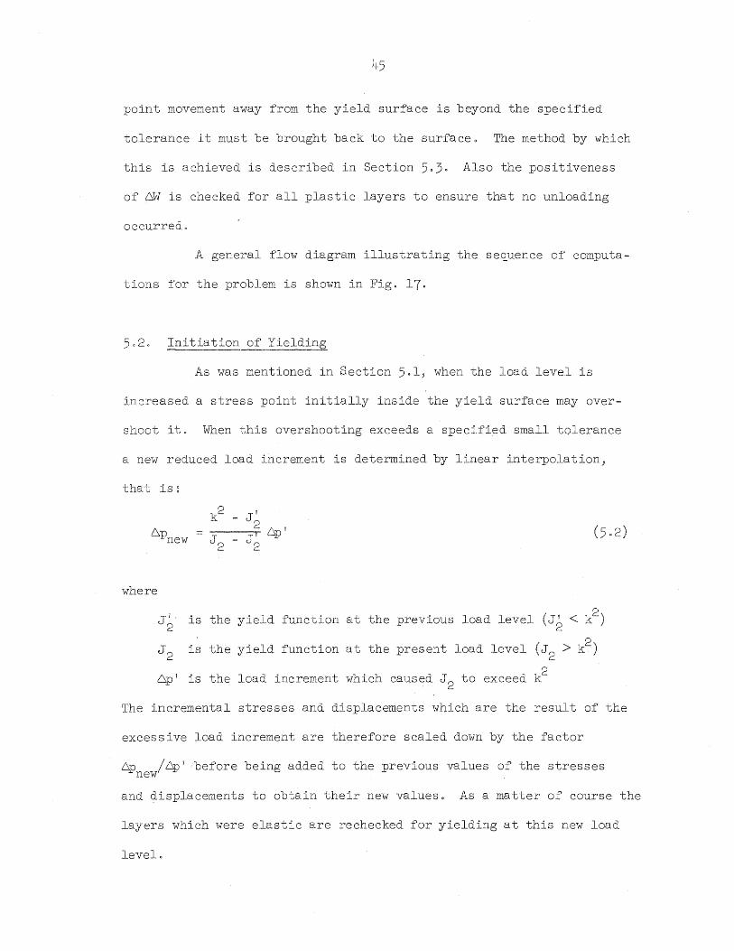
45
point movement away from the yield surface is beyond the specified
tolerance it must be brought back to the surface 0 The method by which
this is achieved is described in Section 5030 Also the positiveness
of 6W 1.s checked for all plastic layers to ensure that no unloading
occurred.
A general flow diagram illustrating the sequence of computa-
tions for the problem is shown in Fig. 17.
5.2. Initiation of Yielding
As was mentioned in Section 5.1, when the load level is
increased a stress point initially inside the yield surface may over-
shoot it . When this overshooting exceeds a speci,fied small tolerance
a new reduced load increment i,s determined by linear i.nterpolat1.on J
that is ~
k2 - JY
L~;Pnew 2 6pf (5.2) J 2 '1i' - tJ2
where
Ji, 2
is the yield function at the previous load level j < k2 ) 2.
J 2 is the yi.eld function at the present load level (J
2 > k2 )
6p! is the load increment which caused J2
to exceed k2
The incremental stresses and displacements which are the result of
excessive load increment are therefore scaled down by the factor
6p /6p l'before being added to the previous values of the stresses new
the
and displacements to obtain their new values. As a matter of course the
layers which were elastic are rechecked for yielding at this new load
level.

46
5 3. Correction Procedure for Plastic Stresses
For the layers which become plastic, the state of stress
represented by a point in the stress space should, under increasing
load, move on the yield surface. However, due to the incremental
nature of the problem, the stress point moves along the tangent to the
surface as shown in Fig. 18. This moves the stress point away from the
2 yield surface J'2 := k "
If the departure exceeds a selected small allowable tolerance
the state of stress must be brought back to the surface or else the
error which keeps accumulating would become excessive. Techniques for
bringing the state of stress back to the yield surface along the gradient
have been used before. (32,23) A different formulation of the same scheme
is developed below.
The yield surface in the case of plane stress is represented
by the quadratic equation:
J 2 1 ( 2 _ 0' 0' + 0' 2) + 1" 2 3' \ O'x X Y Y xy
Let the coordinates of the uncorrected stress point lying outside the
surface be (~ ~ 1" ) The components of the gradient vector to uxl' uyl' xyl'
the surface are:
1 - (20' - 0' ) 3 x y
1 - (20' - 0' ) 3 y x
2'[ , xy
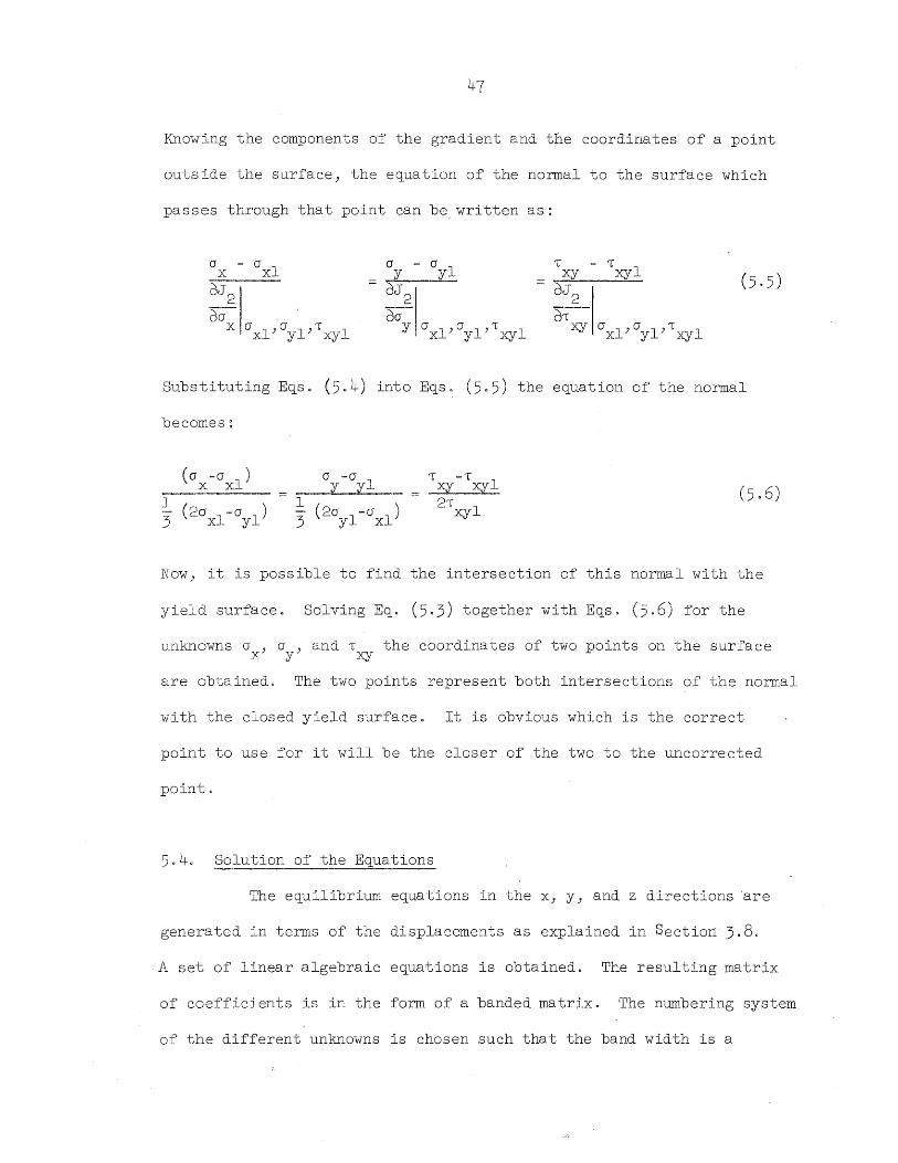
47
Knowing the components of the gradient and the coordinates of a point
outside the surface, the equation of the normal to the surface which
passes through that point can be wri tten as:
(J - (J a - a 1" - 1" xyl x xl y yl xy (5.5) d,J
2 dJ
2 dJ2
dO' dO' ~ x a (J '[ xl) ylJ xyl y a a 1" xl) yl) xyl xy O'xlJO'yl)1"xyl
Substituting Eqs. (5.4) into Eqs. (5.5) the equation of the normal
becomes~
(0' -a 1) x x a -a y yl 1" -'r
xy xyl 21" 1 xy
Now) it is possible to find the intersection of this normal with the
yield surface. Solving Eq. (5.3) together with Eqs. (5.6) for the
unknowns a ) a J and 1" the coordinates of two points on the surface x y xy
are obtained. The two points represent both intersections of the normal
with the closed yield surface. It is obvious which is the correct
point to use for it will be the closer of the two to the uncorrected
point.
5.4. Solution of the Equations
The equilibrium equations in the x) YJ and z directions 'are
generated in terms of the displacements as explained in Section 3.8.
A set of linear algebraic equations is obtained. The resulting matrix
of coefficients is in the form of a banded matrix. The numbering system
of the different unknowns is chosen such that the band width is a

48
minimum. This is done in order to minimize the large number of
quantities to be stored in the core of the computer. A Gauss elimina-
tion method is employed to solve the equations. The computer program
uses an equation solver routine developed by Professor J. W. Melin
which can solve up to 450 simultaneous equations without using
auxiliary storage.
505. Coupling of the Two Systems of the Model
As was mentioned in Section 2.1 the model, as used in this
study) can be considered as a supe+position of two systems of
Schnobrichis model. Figure 19 shows one system with solid circles) the
other with hollow circles. In the elastic range, the equilibrium
equations of one system are independent of those of the other system.
In spite of this the solutions for the two networks were found(27) to
be in good agreement with one another for the case where all four
boundaries are simply supported. When two opposite edges _are free and
the remaining two opposite edges simply support.ed the agreement b'etween
the two systems is not quite as good. The deflection along the free
edge is found to oscillate between the two systems) Fig. 24. Also if
the deflection along a diagonal of o,ne quadrant of the shell is plotted,
proceeding from the free edge to the simply supported one, it is found
that the oscillations are noticeable close to the free edge but damp
out near the simply supported edge) Fig. 25. This phenomenon occurs in
the case of the free edge because the free edge is sensitive to the
number of grid spacings used, and in effect one system is being solved
with a finer mesh than the other. As the fineness of the grid is

49
increased the results pertaining to the two systems move closer to
each other and the oscillation becomes less pronounced.
In the plastic range) the eCluilibrium eCluations of the two
systems are coupled as can be seen from the operators in Figs. 10) 11)
and 120 Even when yielding starts in one system the relative magni
tude of the oscillation does not seem to grow much larger although
its absolute magnitude does.
In the case of a multiple barrel shell simply supported at
both ends the agreement between the two systems in the elastic range
is Cluite good and the oscillations are hardly noticeable 0 In the
plastic range the oscillations become more pronounced. Figure 35 shows
the deflection along a diagonal of one Cluadrant of the shell. Several
curves are;plotted to show the behavior at different load levels.

6. NUMERICAL RESULTS
6.1. General Remarks
Two illustrative problems are presented in this chapter to
demonstrate the success of the model for handling the elasto-plastic
analysis of shells. The first problem is that of a cylindrical shell
with the transverse edges simply supported and the longitudinal edges
free. The second problem is that of a continuous multiple barrel
shell. In both cases the loading applied is a uniform increasing load
of intensity p lb/ft2 , The loading and geometry are symmetrical about
both axes of the shell, so only one quandrant is needed to solve the
problems.
Previous work in the area of shell structure analysis is) in
general) limited to linearly elastic material behavior. Although some
work has been done on the basis of limit analysis it is mostly re-
stricted to rotationally symmetric shells. Thus comparisons with
previous works are of necessity quite limited.
6.2. Cylindrical Shell with Two Edges Simply Supported and the Remaining Two Free
The shell considered here is a single bay shell simply
supported at both its transverse ends while the longitudinal straight
edges are free. The"dimensions of the shell are chosen to correspond
to those of Example 1 in the ASCE Manual 31. (8) These dimensions are
given in Fig. 20. The ratio R/L for this shell is 0.5. Cylindrical
50

51
shells are usually described on the basis of this ratio as either long,
intermediate) or short. Manual 31 does not make such a fine distinction
and categorizes shells as either short or long. The division point
between short and long shells occurs at the ratio R/L = 0.6. According
to Gibson(15) the shell chosen in this example would be classified an
intermediate shell. The classification of the shells as made by various
authors is an attempt to distinguish between shells whose primary
action l.S that of a beam from those whose primary action is arching.
For this study the intermediate case was chosen in order that the shell
have both actions present.
A quadrant of the shell is divided into six spacings in each
direction) resulting in 234 unknowns. Pol.sson 1 s ratio is chosen to be
zeroo The yield stress a is chosen on the basis of the maximum o
longitudinal tensile reinforcement in a reinforced concrete shell. For
the Manual 31 shell this is about 8% of the sectional area. Thus if
the material is considered homogeneous, as is done in this study, an
equivalent yield stress may be assumed. If the yield stress for steel
is 33 ksi, i.e., 47.5 x 10⁵ lb/ft2 then the equivalent yield stress is
3.8 x 10⁵ lb/ft2
. In this case t~e yield limit in simple shear
k = 2018 x 105 lb/ft2
. But since the top and bottom stresses in the
model are in terms of lb/ft) then a and k are multiplied also by h/2. (,~ 0 -
If kh/2is designated ilSK" then the" selected tolerance for yielding is
2 + 0.01 SK .
A unit load was applied to,the shell and increased to get the
first layer of a node to yield. Subsequent loading was then progres-
sively increased, successively forcing further layers to yield. At an
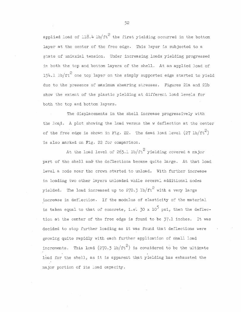
52
applied load of 118.4 lb/ft2 the first yielding occurred in the bottom
layer at the center of the free edge. This layer is subjected to a
state of uniaxial tension. Under increasing loads yielding progressed
in both the top and bottom layers of the shell. At an applied load of
154.1 lb/ft2
one top layer on the simply supported edge started to yield
due to the presence of maximum shearing stresses. Figures 21a and 21b
show the extent of the plastic yielding at different load levels for
both the top and bottom layers.
The displacements in the shell increase progress i.vely with
the 10a1,do A plot showing the load versus the w deflection at the center
of the free edge is shown in Fig. 22. The dead load level (27 lb/ft2 )
'is also marked on Fig. 22 for comparison.
At the load level of 263.1 lb/ft2 yielding covered a major
part of the shell an&' the deflections became quite large. At that load
level a node near the crown started to unload. With further increase
in loadi.ng two other layers unloaded while sev:eral additional nodes
yielded. The load increased up to 270.3 lb/ft2
with a very large
increase in deflection. If the modulus of elasticity of the material
is taken equal to that of concrete -' i. eO .. 30 x 105 psi, then the deflec
tion at the center of the free edge is found to be 37.1 inches. It was
decided to stop further loading as it was found that deflections were
growing quite rapidly with each further application of small load
increments. This load (270.3 lb/ft2 ) is considered to be the ultimate
load for the shell, as it is apparent that yielding 'has exhausted the
major portion of its load capacity.

53
A plot of the normal deflection) w) on the section at midspan
between the two simply supported edges is shown in Fig. 23 for the
different load levels. Also the deflections along the free edge and
along a diagonal proceeding from the free edge to the simply supported
edge are shown in Fig. 24 and Fig" 25. The variations of the longi-
tudinal force N at the midspan section and along the free edge are x
shown in Fig. 26 and Fig. 27 respectively. From Fig. 26 it is noticed
that with the increase in loading and plastic action the position of
the neutral axis moves'upward towards the crown. Also,in the later
f
stages of loading the stresses on the tension side become almost constant
and equal to the yield value in simple tension" On the other hand" the
stresses on the compression side cannot reach as high a value as the
yield stress since in this zone high transverse stresses occur due to
the bendi.ng moment M. If an ideal stress distribution is assumed) Wl th Y
the stress in compression assumed to be half the stress in tension) the
position of the neutral axis corresponds to 1/3 the angle cp measured
from the edge. The obtained ultimate load is then 331.1 Ib/ft2. If
the stress in compression is assumed to be one third the stress in
tension the pos i tion of the neutral axis' corres<ponds to 1/4 the angle cp
measured from the edge. The obtained ultimate load would then be
261.3 Ib/ft2. This latter value corresponds quite well with the
ultimate load obtained in this study. The shearing force N along the xy
simply supported edge is shown in Fig. 28. Finally) the variation of
the transverse bending moment M at the midspan section is shown in . y
Fig. 29 for different load levels.

54
The displacements and forces in the elastic range agree with
those obtained by Mohraz and Schnobrich. (27) Small differences do
occur since in this study cos ~/2 is taken to be equal to unity. The
results obtained agree quite well with those given by the ASCE
Manual. (8) The largest deviation is in the magnitude of the N force x
at the center of. the free edge. For the 6 x 6 grid this N force for x
a unit load is 886 Ib/ft, while for an 8 x 8 grid it is 949 Ib/ft.
The corresponding value of N obtained from the Manual is 1128 Ib/ft. x
The value of N at the edge converges to the Ifexacti! value as the mesh x
becomes finer. If linear extrapolation is used the value of N when x
the grid size tends to zero is 1030 Ib/ft. It should be kept in mind
that the values obtained from the Manual are for a sinusoidal load
which causes the N stress at midspan section to be slightly larger x
than that resulting from a uniform load. A plot of the N force at x
midspan section comparing the results obtained here with those of the
Manual is shown in Fig. 30.
Almost no information exists on which to draw comparisons
with the results of this study once plastic action has begun in the
shell. The small amount of experimental data thatJhas been published
deals with reinforced concrete and microconcrete models.(3,4,5) In these
experiments transverse bending moments develop yi.eld line hinges in the
shell surface. The model in this study is considered composed of iso-
tropic materials. Choice of the yield properties of the nodes was
guided by considerations bf th~ usual longitudinal tensile steel near
·the free edge. As a consequence, the resulting transverse moment re-
-si-stance i.s cons iderably. higher ~han for: most normally reinforced concrete
55
shells) suppressing any tendency to form yield line hinges. This dis-
crepancy between the model and reinforced shells was realized at the
outset of the study. However) as subsequently discussed in Chapter 7)
it was decided not to overly complicate the programming effort of this
first study. Any comparisons with the limited number of published
experimental data must therefore be of a rather gross qualitative)
rather than quanti.tative., nature.
A rigid-plasti.c analysis of circular cylindri.cal roof shell
t t f d b Fl'a.lko. (14) F' lk ht d 1 s ruc ures was per orme yl.a 0 soug upper an ower
bounds to the ultimate load of the shell when loaded by uniform radial
pressure. The yield condition used was a linear yield condition which
approximated both the Mi.ses and Tresca conditions. The shear stress
does not combine in any of the inequalities of the yield condition)
rather) additional bounding planes at T xy + k were used. Fialko
assumed three different stress fi.elds to get lower bound solutions)
selecting the largest. He also assumed three different kinematical
fields to obtain upper bound solutions and selected the lowest. All
lower bound solutions obtained according to the three assumed stress
fields fall below the ultimate load as determined in this investigation.
YwO of the kinematical fields give upper bounds which lie above the
ultimate load. A third kinematical field gives a load which falls
below the ultimate load obtained in this study. This third kinematical
field does not reflect an increase in the ultimate load when the opening
angle ~ increases. This is not the case for the type of shell analyzed
in which beam type failure is prominent. The difference in loading
and yield conditions between the two methods of analys is i.s another
factor which results in that discrepancy. To investigate the effect of
the difference in loading the example presented here is examined for
the case of uniform radial loading. This is carried out till the end
of the elastic range. For radial loading the transverse moments are
higher throughout the shell than those resulting from vertical loading.
Also the axial tensile force N at the free edge is larger for the shell x
subjected to radial loading. Consequently the end of the elastic range
is 11202 Ib/ft2 for radial loading versus 118.4 Ib/ft2 for vertical
loading. Higher transverse moments and axial force at the free edge
will cause the ultimate load to drop. Fialko 1 s third kinematical field
is based on the assumption that yield lines will form parallel to the
longitudinal edge. Even when the loading and yield conditions used by
Failko are incorporated in the computer program of this study it is in-
conceivable that such yield lines would form. This is simply because
the transverse moment is not high enough to form plastic lines parallel
to the longitudinal edges.
To investigate the effect of the gri.d size on the solution
an 8 x 8 mesh on one quadrant is also used. The resulting number of
unkBowns is 408. The problem was run on thk computer for 51 cycles of
incremental loading. After these 51 cycles the load had reached the
2 value of 238.8 Ib/ft. The obtained load deflection diagram and yield
pattern are almost identical to those obtained from the problem with
6 x 6 grid when compared at the corresponding load level. Thus it is
felt unwarranted to run the problem with the finer mesh up to the
ultimate load. Any difference between the two ultimate loads is expected
to be very small. This can be explained by the fact that the shell is

57
behaving like a beam. Near the ultimate load a plastic hinge is formed
at the center of the shell. The distribution of the longitudinal force
N does not change significantly by decreasing the grid size. x
Convergence has been demonstrated for similar models and
" similar elasto-plastic analysis in the investigations by Lopez and
Ang(24) for square plates) Mohraz and Schnobrich (2~) f:or shell structure~,
and by Crose and Ang(7) for circular plates considering large deflection
effectso In view of these earlier studies no additional investigation
is considered necessary for this study.
6030 Mul ti.ple Barrel Shell Simply Supported at Both Ends
The dimensions and the material properties of the shell in this
case are the same as those used in Section 6.2 for the single barrel
shell. A quadrant of the shell i.8 divided into six spacings in each
direction resulting in 222 unknowns. The shell is subjected to an in-
creasing load. The first yielding occurs in the bottom layer at the
cent~~ of the valley at a load of 188.3 Ib/ft2
. With further loading
yielding progresses in both the top and bottom layers of the shell.
Figure 31 shows this progression. Once the load passes the value of
about 400 Ib/ft2 yielding spreads rapidly unti.l it covers the major
portion of the shell.
In the case of a multiple barrel shell the maximum deflection
is not at the center of the continuous edge but is shifted away from it
by about 1/3 of the angle cpo A plot of the load p versus w i.8 shown max
in Fig. 32. In the last stages of loading the slope of the load
deflection curve becomes very flat) and any small load increment causes

58
the deflections to increase appreciably. At the load level of
45201 lb/ft2
computations are stopped and this load is considered to be
the ultimate load for the shell. If as in Section 6.2 the modulus of
elasticity of the material is considered equal to that of concrete,
then the maximum deflection for the load 452.1 lb/ft2 is found to be
13.1 inches. At this load level the majority of the top layers and a
substantial number of the bottom layers have already yielded.
A plot of the displacement w at the midspan section is shown
i.n Fig. 330 Also the displacement w along the valley and along a
diagonal proceeding from the continuous edge to the simply supported
edge is, shown in Fig. 34 and Fig. 35 respectively. The plot of the
displacement along the diagonal shows that, as plasti.c flow progresses)
os cilla ti.ons between the two systems of nodes develop. This phenomenon
has been explained previously in Section 5.5.
The variation of the force N at the midspan section is shown x
in Figo 36. This closely resembles the ideal plastic stress distribu-
tion in the case of beams. If this ideal stress distribution is applied
to the shell, i.e. equal tension and compression stresses and a
position of the neutral axis corresponding to 1/2 the angle ~, the
obtained uitimate load is 451.6 lb/ft2
. This is in very close agree-
ment with the computed value. Figure .37 s·hows the variation of the N x
force along the valley. Once yielding takes place redistribution of the
stresses is possible. In this cas~) when the N force decreases in a x
certa in portion along the valley ) it i.ncreases along a line parallel to
and one spacing away from the valley. The shearing force N along the xy
simply supported edge is shown in Fig. ·38.
59
The bottom layers in the midspan section are in a state of
biaxial compression. Once these layers yield the stresses in the
y-direction decrease to allow for the increase in the stresses in the
x-direction so that the state of stress remains on the yield surface.
This reduction in the stresses in the y-direction causes the trans-
verse moment M to decrease once plastic flow occurs. The variation y
of the transverse moment M at the midspan section for different load y
levels is shown in Fig. 39. 0 The reduction of M can be explained by y
the fact that the N x
force becomes almost constant on both sides of
the midspan section. JOust as in any beam, the shearing force, N J xy
cannot develop where there is no change in the longitudinal force.
Thus the transverse moment decreases since it depends on the shear
difference between the two transverse sections. The values of N ,N , x xy
and M for the nodes of one system of the model are listed in Tables 1, y
2, and 3 respectively.
In the elastic range the maximum displacement w in the case
of the multiple barrel shell is about one-tenth the value of the maxi-
mum displacement in the shell with free edges. At the ultimate load,
the maximum displacement w in the case of the multiple barrel shell is
about one-third the value of the maximum displacement in the shell with
free edges. The ultimate load itself for the multiple barrel shell is
1067 times that for the single barrel shell. It is thus evident that
the multiple barrel shell is. far more satisfactory in its serviceability
and strength than the single barrel shell.

7e CONCLUSIONS AND RECOMMENDATIONS FOR ~JTURE STUDY
The model used in this investigation proved to be successful
in handling the analysis of elasto-plastic shells. It simulates a
laboratory test through which the behavior of the shell is studied.
Laboratory tests are) in general, expensive and cannot cover a wide
range of varying parameters. However, such a wide range can be directly
covered on the computer by simply varying the input data. The numerical
method used proved to be efficient and suitable for programming.
The results obtained for the problems presented ps illustra
tive examples above show clearly that the multiple barrel shell~is
far better than the si,ngle barrel shell in both servicability and
ultimate strength. Although the model was used here to solve cylindrical
shells it is capable of solving elliptic paraboloids and hyperbolic
paraboloids. To arrive at appropriate solutions for these shells
entails minor ohanges in the computer program. Solving such problems
will be of interest especially since these shells are usually more
uniformly reinforced than are cylindrical shells. Due to this uni
formity the obtained results would closely resemble the true behavior
of the shells.
In order to provide for the variations in reinforcing steel
quantities and placement, orthotropy of the individual nodal layers
would be necessary. Also, allowance for differences in the properties
of the top and bottom layers at each node would have to be included, as
would the variations in the properties with the surface coordinates of
60

61
the shell. The inclusion of such differences of material properties
for different points of the shell does not pose any difficulty in the
theory of application of the model. It does) however, represent a
significant programming effort.
Another possible further study is to alter the model to
account for the behavior of both the concrete and the steel embodied
in it. This could be achieved by changing the formation of the nodes.
Yield conditions for reinforced concrete(28,30 ) and for orthotropic
materials can then be used.
The study should also be extended to the large deflection
theory of shells to account for the changes in geometry occurring under
heavy loading conditions. Such a study is not necessary for the type
of cylinders investigated here, but would be for shallow doubly curved
shells where signi.ficant changes in the radii of curvature mi.ght occur.
The boundary conditions of a supporting edge beam should be
developed such that it would be possible to trace yielding in both the
beam and the shell together.
In conclusion.? to achieve the most economical design of shell
roofs the methods of analysis should be based on an understanding of
all stages of shell behavior. This study of elasto-plastic shell roofs
constitutes an important step towards the realization of this goal.
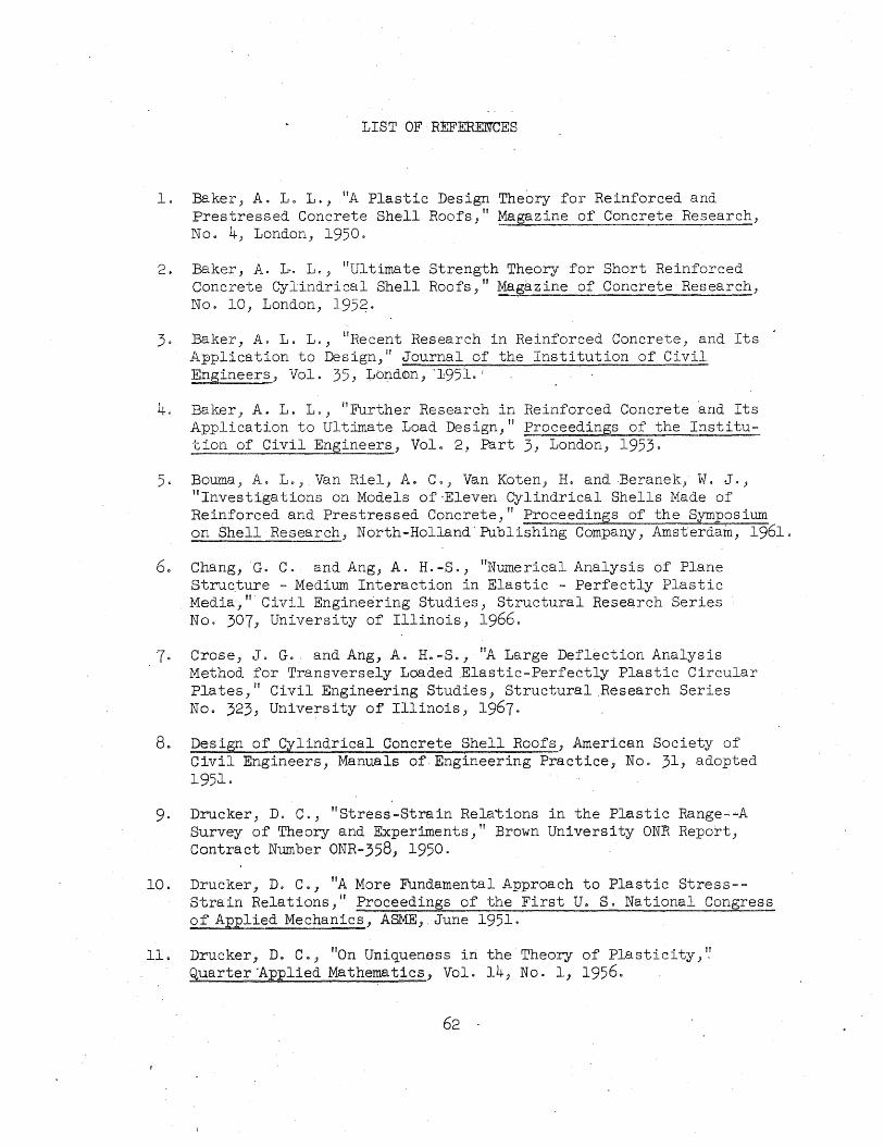
LIST OF REFERENCES
1. Baker, A. L 0 L., "A Plastic Design Theory for Reinforced and Prestressed Concrete Shell Roofs," Magazine of Concrete Research, No.4, London, 1950.
2. Baker, A. L·. L., "Ultimate Strength Theory for Short Reinforced Concrete Cylindrical Shell Roofs," Magazine of Concrete Research, No. 10, London, 1952.
3. Baker, A. L. L., "Recent Research in Reinforced Concrete, and Its Application to Design,lI Journal of the Institution of Civil Ensineers, Vol. 35, Londcbn,'1951.·
4. Baker, A. L. L., "Further Research in Reinforced Concrete ·and Its Application to Ult.imate Load Design," Proceedings of the Institution of Civil Engineers, Vol. 2, Part 3, London, 1953.
5. Bouma,A. Lo, Van Riel, A. C , Van Koten, H. and Beranek, W. J., "Investigations on Models of "Eleven Cylindrical Shells Made of Reinforced and Prestressed Concrete," Proceedings of the SyPlposium on Shell Research, North-Holland·Publishing Company, Amsterdam, 1961.
6. Chang,G. C. and Ang, A. H. -S., "Numerical Analysis of Plane Structure - Medium Interaction in Elastic - Perfectly Plastic
. Media, II Civil Engineering Studies, Structural Research Series No. 307, University of Illinois, 1966.
7. Crose, J. G. and Ang, A. H.-S., "A Large Deflection Analysis Method for Transversely Loaded Elastic-Perfectly Plastic Circular Plates," Civil Engineering Studies, Structural Research Series No. 323, University of Illinois, 1967.
8. Design of Cylindrical Concrete Shell Roofs, American Society of Civil Engineers, Manuals of Engineering Practice, No. 31, adopted 1951.
9. Drucker, D. C., "Stress-Strain Relations in the Plastic Range--A Survey of Theory and Experiments," Brown University ONl1 Report, Contract Number ONR-358, 1950.
10. Drucker, D. C., "A More Fundamental Approach to Plastic Stress-Strain Relations," Proceedings of the First U. S. National Congress of Applied Mechanics, ASME, June 1951.
11. Drucker, D. C., "On Uniqueness in the Theory of Plasticity,'.' Quarter "Applied Mathematics, Vol. 14, No.1, 1956.
62

12. Drucker, D. C., I!A Definition of Stable Inelastic Material,l! Journal of Applied Mechanics) Vol. 26, March 1959.
13. Drucker, Do C., "Plasticity," Proceedings of the First Symposium on Naval Structural Mechanics, ed. J. N. Goodier and N. J. Hoff, Pergamon Press, New York, 1960.
14. Fialkow, M. No) "Limit Analysis of Simply Supported Circular Shell Roofs,!! Journal of the Engineering Mechanics Division, Proceedings of ASCE, VoL 84, J:uly 1958.
15. Gibson, J. Eo, The Design of Cylindrical Shell Roofs, D. Van Nostrand Company, New J"ersey, 1961.
16. Golrdenv~ize~, A. L., Theory of Elastic Thin Shells, Pergamon Press, New York, 1961.
17. Handelman, G,. H. and Lin, C. C. J nOn the Mechanical Behavior of Metals in the Strain Hardening Range," ~uarter of Applied Mathematics, Vol. 4) 194 7"
18. Harper, G. N. and Ang, Ao Ho-S., !fA Numerical Procedure for the Analysis of Contained Plastic Flow ProblemS," Civil Engineering Studies, Structural Research Series No. 256, University of Illinois, 1963.
19. Hill, R., The Mathematical Theory of Plasticity, Oxford University Press, London, 1950.
20. Hodge} P. G., Jr., Limit Analysis of Rotationally Symmetric Plates and Shells, Prentice-Hall, New Jersey, 1963.
21. Johansen} K. W., "Critical Notes on the Calculation and Design ,of Cylindrical Shells,fI Third Congress of the International Association for Bridge and Structural Engineers, Final Report, 1948.
22. Lame, G. and Clapeyron, Eo, IIMemoires Sur L'Equilibre Interiur Des Corps Solides Homogenes," Memoires Presente8 A L'Academie Des Sciences De LVlnstitut De France; second series, Vol. 4, 1828.
I
'23. Lopez, L. A.) !fFlex11ral Analysis of Elastic-Plastic Rectang'ular Plates,fJ Ph.D. Thesis" University of Illinois, May 1966.
~
24. Lopez, L. A. and Ang, A. H. -S., If Flexural AnalYSis of ElasticPlastic RectangUlar Plates,Tr Civil Engineering Studies, Structural Research Series No. 305, UniverSity of IllinoiS, 1966.
25. Lundgren, H., Cylindrical Shells, Danish Technical Press, Copenhag~n, 1951.
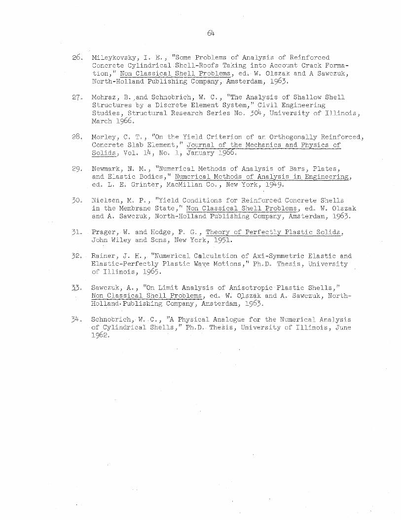
64
26 0 Nileykovsky, I. Eo J !!Some Problems of Analysis of Reinforced Concrete Cylindrical,Shell-Roofs Taking into Account Crack Formation," Non Classical Shell Problems, edo W. Olszak and A Sawczuk, North-Holland Publishing Company, Amsterdam, 1963.
270 Nohraz -' B. )and Schnobrich, w. C., YfThe Analysis of Shallow Shell Structures by a Discrete Element System,n Civil Engineering Studies, Structural Research Series No. 304, University of Illinois, March 19660
28. Morley, Co To, flOn the Yield Criterion of an Orthogonally Reinforced, Concrete Slab Element,1I Journal of the Mechanics and Physics of Solids) Vol. 14, Noo 1, January 19660
290 Newmark, N. M. J HNumerical Methods of Analysis of Bars, Plates, and Elastic Bodies,iI Numerical Methods of Analysis in Engineering, edo Lo Eo Grinter, MacMillan Coo, New York, 19490
300 Nielsen, Mo Po, YfYield Conditions for Reinforced Concrete Shells in the Membrane State,ir Non Classical Shell Problems, edo Wo Olszak and A. Sawczuk, North-Holland Publishing Company, Amsterdam, 19630
310 Prager, Wo and Hodge, Po Go J Theory of Perfectly Plastic Solids, John Wiley and Sons, New York, 1951.
320 Rainer, J. H. J f'N'umerical Calculation ofAxi=Symmetric Elastic and Elastic-Perfectly Plastic Wav;e Motions," PhoDo Thesis, University of Illinois, 1965.
3j. Sawczuk, Ao, nOn Limit Analysis of Anisotropic Plastic Shells,lI Non Classical Shell Problems, edo W. O~lszak and AD Sawczuk, NorthHolland~ Publishing Company} Amst-erdam, 196.30
34. Schnobrich} \AL C., "A Physical Analogue for the Numerical Analysis of CYlindrical Shells,ft PhoD. Thesis, University of Illinois, J'une 1962.

TABLE 1.
~ 1 3
1 -38.2 -36.6 3 -36.8 -35.4 5 -32·9 -31·7 7 -26.7 -26.0 9 -18·7 ;"18.4
11 -9.6 -9·5 13 0 0
1 -105·9 -107·1 3 -103·7 -103·7 5 -95·9 -93·1 7 -80·9 -75·7 9 -58.2 -53.5
11 -30·3 -27·7 13 0 0
J
1 -123·1 -124·9 3 -119.4 -122.6 5 -113·0 -118.0 7 -102.4 -97·0 9 -75·7 -68·7
11 -40.5 -35·9 13 0 0
* LONGITUDINAL FORCE N (lb/ft) x
p = 188.3 1b/ft2
5 7 9 11
-30·5 -16.5 8.5 46.2 -29·6 -16·3 7·9 44.8 -27·0 -15·5 6.4 40.7 -22·7 -13.8 4.1 33·9 -16.6 -10·9 1.6 24.4 -8.8 -6.3 -0.08 12·5 0 0 0 0
j: l;
p = 412.8 1b/ft2
-92.0 -26.4 106.5 110·5 -85.6 -24.8 93.8 116.0 -70·9 -19·5 60.9 117.4 -55·0 -15·3 39·7 93·7 -38·3 -11.8 23·7 62.7 -19·9 -7·1 9.8 30·7 .
0 0 0 0
p = 452.1 lb/ft2
-125·5 20.8 112.4 115.4 -124.0 25.4 108.2 115.1 -93·5 8.1 94.7 116.0 -66.1 1.4 62.1 109·3 -43·6 -2·7 40.6 74·3 -21·9 -3·3 22.0 32.8
0 0 0 O·
* All numbers to be multiplied by 103
JA
13 11
9 7 5 3
y cant.
S.S
1 x 1 3 5 7 9 11 13 IA
13
96.1 93·9 87.2 75·7 58.6 34·3
0
112.4 112·3 106.4 106.3 92.6 58.8
0
114.0 115·0 98.2 83.0 76.0 53·3
0

b 1
1 0 3 0 5 0 7 0 9 0
11 0 13 0
1 0 3 0 5 0 7 0 9 0
11 0 13 0
J 1 0 3 0 5 0 7 0 9 0
11 0 13 0
66
* TA.BLE 2. SHEARING FORCE N (lb/ft) xy
p = 188.3 Ib/ft2
3 5 7 9
0 0 0 0 -1.8 -3·3 -3·9 -3·3 -3·5 -6.4 -7·9 -7.4 -5·0 -9·2 -11.8 -11·7 -6.1 -11·5 -15·2 -15·9 -7·0 '-13·4 -18,0 -19.6 -7.6 -15·7 -23·0 -25·3
p = 412.8 Ib/ft2
0 0 0 0 -3·5 -11·7 -18.2 -4.0 -8·5 -19·6 -27·0 -22.1
-13·5 -26·3 -33·9 -30·3 -17·8 -32.0 -39·0 -36.8 -20·9 -36.9 -43· 5 -42.0 -22.8 -44.7, -60·9 -56.1
p = 452.1 Ib/ft2
0 0 0 0 -1·3 -4.5 -28·3 -1.4 -5.6 -22·5 -37·6 -16·3
-14·3 -31.9 -42·3 -34.3 -20·9 -36.8 -45·4 -41.3 -26.2 -43·5 -50.4 -40·3 -35·1 ... 64·3 -68.3 -64.5
* All numbers to be multiplied by 103
JA+ Y cant.
~? t T T ~ T ~ ~ 1.1.
9 7 5 3
S.S.
11 3 5 7 9 11 13 IA x
11 13
0 0 -1.6 0 -4·7 0 -7·9 0
-11·7 0 -16.5 0 -16.1 0
0 0 -2.8 0 -1.2 0
-10·7 0 -21·9 0 -34.4 0 -24.4 0
0 0 -8.5 0 -6.7 0 -9·7 0
-22.1 0 -38.7 0 -7~6 0
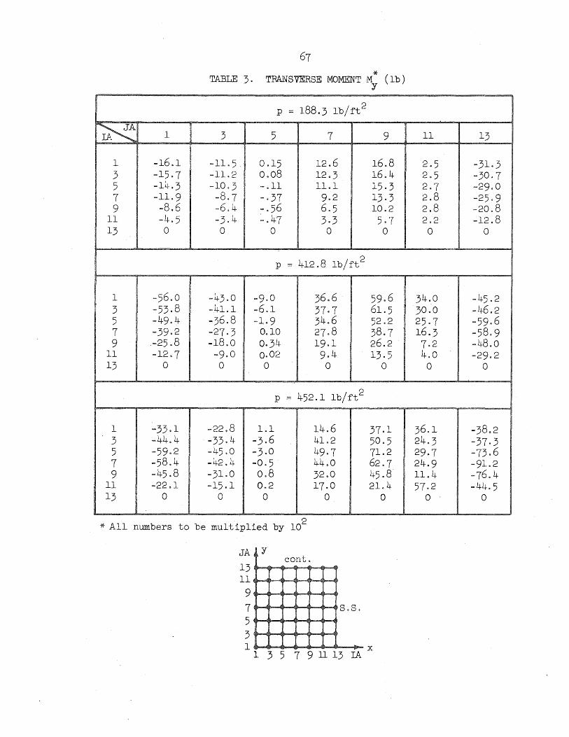
~ 1
1 -16.1 3 -15·7 5 -14.3 7 -11·9 9 -8.6
11 -4.5 13 0
1 -56.0 3 -53.8 5 -49.4 7 -39·2 9 -25.8
11 -12·7 13 0
1 -33·1 3 -44.4 5 -59.2 7 -58.4 9 -45.8
11 -22.1 13 0
* TABLE 3. TRA.l~SVERSE MOMENT M (lb) y
p = 188.3 1b/ft2
3 5 7 9
-11·5. 0.15 12.6 16.8 -ll.2 0.08 12·3 16.4 -10·3 -.11 11.1 15·3 -8.7 -·37 9·2 13·3 -6.4 -.56 6.5 10.2 -3.4 ~.47 3·3 5·7 0 0 0 0
p = 412.8 lb/ft2
-43.0 -9·0 36.6 59.6 -41.1 -6.1 37·7 61.5 -36.8 -1·9 34.6 52.2 -27·3 0.10 27·8 38.7 -18.0 0.34 19·1 26.2 -9·0 0.02 9.4 13·5 0 0 0 0
p = 452.1 lb/ft2
-22.8 1.1 14.6 37.1 -33.4 -3.6 41.2 50·5 -45.0 -3·0 49.7 71.2 -42.4 -0·5 44.0 62.7 -31.0 0.8 32.0 45.8 -15·1 0.2 17·0 21.4
0 0 0 0
* All numbers to be multiplied by 102
JA Y cant.
13 ~t--4I~--.. ............. 11~~~-....-.... ..... 9~~~ ..................... -. 7 5 3
+-~~S.S.
1 x 1 3 5 7 9 11 13 lA
11 13
2·5 -31·3 2.5 -30·7 2·7 -29·0 2.8 -25·9 2.8 -20.8 2.2 -12.8 0 0
34 .. 0 -45.2 30.0 -46.2 25·7 -59.6 16.3 -58.9 7·2 -48.0 4.0 -29·2 0 0
36.1 -38.2 24.3 -37·3 29.7 -73.6 24.9 -91.2 11.4 -76.4 57·2 -44.5
0 0
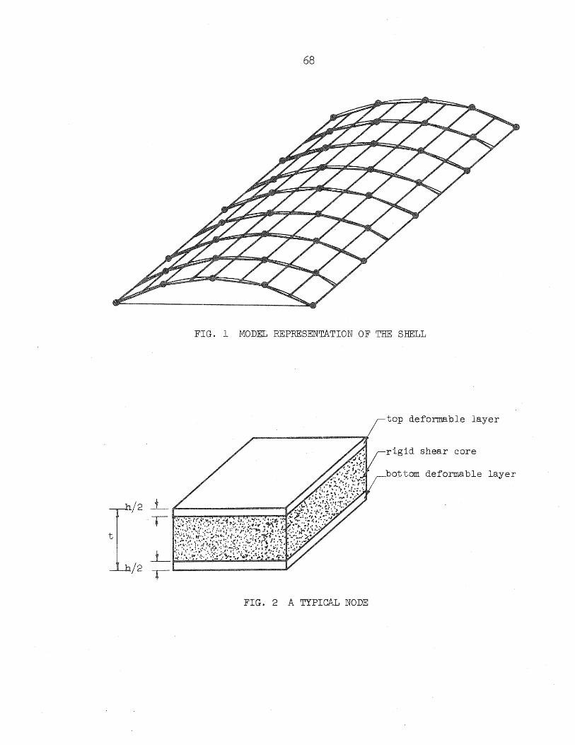
68
FIG. 1 MODEL REPRESENTATION OF THE SHELL
top deformable layer
rigid shear core
bottom deformable layer
t
FIG. 2 A TYPICAL NODE

x
I· L ~j x
i-2 1-1 i i+1 i+2
FIG. 3 GRID POINT IDENTIFICATION AND LOAD CONTRIBUTION AREAS
FIG. 4 COORDINATE AXES AND DISPLACEMENTS

70
y~ ....
FIG. 5a POSITIVE DIRECTIONS OF THE STRESSES
y x
FIG. 5b POSITIVE BENDING MOMENTS
y x
FIG. 5c POSITIVE TWISTING MOMENTS
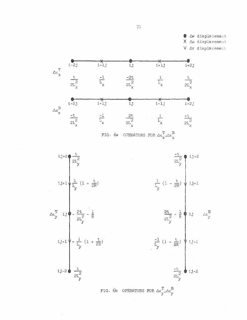
6ET x
6EB x
ij+2
ij+1
ij -1
ij-2
71
, ~
, ~
i-2j i-1j ij i+1j
t -1 -2t 1
212 1 212 L x x x x
, ~
, ~
i-2j i-1j ij i+1j
-t -1 2t 1
2L2 L 212 L x x x x
FIG. 6a OPERATORS T B FOR DE ,DE X X
1 t 1 (1 + 2R)
Y
2t 1 -+ -2L2 R
Y
1 t - L (1 + 2R) Y
-1 t (1 - -) L 2R
Y
T B FIG. 6b OPERATORS FOR DE ,DE Y Y
, DW disp1acemeut
X DU disp1acemen t
V DV disp1acemen!-,
, i+2j
t
212 x
, i+2j
J.. -L,
2L2 x
ij+2
lj+1
ij
ij-1
ij-2
B DE
Y
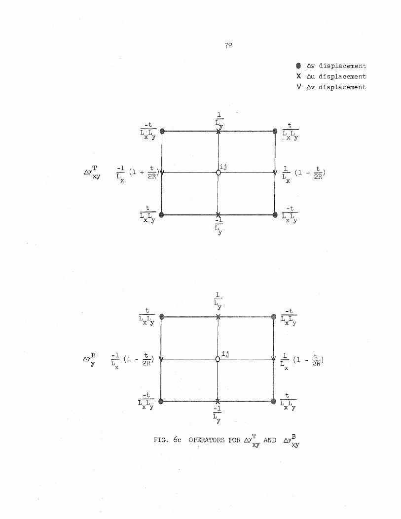
-t L L x y
t L'L x y
t L'L xy
-1 (1 _ ~) L 2R x
-t L'L x y
',I
l1li>.
F'
, J
1 L ,J/ ...
72
ij "\ ~
:""1 L
Y
1 L
Y .(
if'
I
., -1 L
y
ij
\ II
\ II
t
• !:::.W displacement
X !:::.u displacement
V !:::.V displacement
L L ..x y
-t L L
x y
-t L L x y
1 L
x
t (1 - -) 2R
t L'L x y
FIG. 6c OPERATORS FOR !:::.IT AND !:::.lB xy xy

a x
73
T xy
a .. y
FIG. 7a VON MISES YIELD SURFACE FOR A STATE OF PIANE STRESS
a y
FIG. 7b YIELD LOCUS IN CASE ~ = 0 xy
'T xy
FIG. 7c YIELD LOCUS IN CASE 0y"= 0
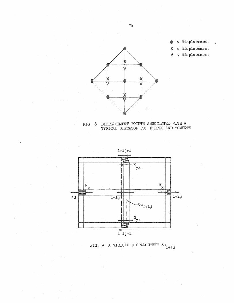
74
• w displacement
X u displacement
V v displacement
FIG. 8 DISPLACEMENT POINTS ASSOCIATED WITH A TYPICAL OPERATOR FOR FORCES AND MOMENTS
i+lj+l
i+lj-l
N x
FIG. 9 A VIRTUAL DISPLACEMENT oU i +1j
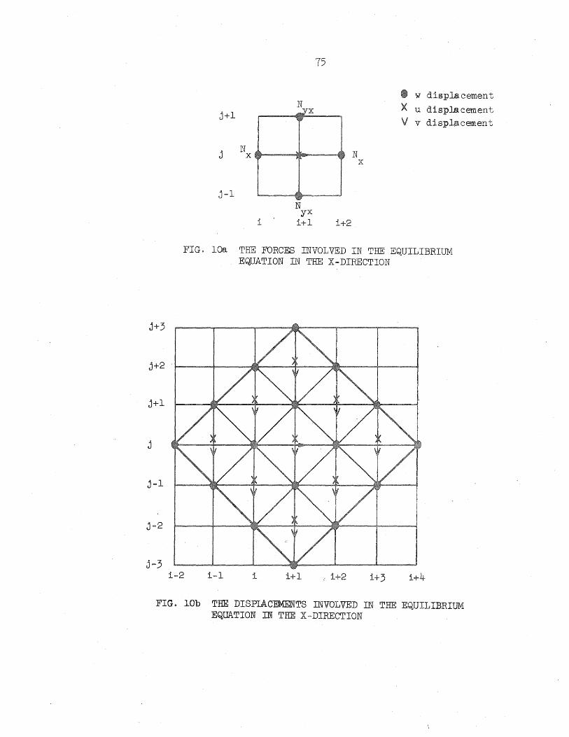
j+3
j+2
j+l
j
j-l
j-2
j-3
j+l
j
j-l
N x 'Ii,.
i
N .:::IX ~"
jJ
<II
~II"
N yx
i+l
75
.Alii
i+2
N x
• w displacement
X u displacement
V v displacement
FIG. lOa THE FORCES INVOLVED IN THE EQUILIBRIUM EQUATION IN THE X-DIRECTION
i-2 i-l 1 1+1 1+2 1+3 i+4
FIG. lOb THE DISPLACEMENTS INVOLVED IN THE EQUILIBRIUM EQUATION IN THE X-DIRECTION

j+4
j+2
j+l
j
j-l
j-2
j+2
j+l
j
N M xy' xy .11'
i-l
N ,M Y Y
. ., N ,M Y Y
i
11 N M xy' xy
i+l
• VI displacement
X u displacement
V v displacement
FIG. lla THE FORCES AND MOMENTS INVOLVED IN THE EQUILIBRIUM EQUATION IN THE Y-DIRECTION
i-3 i-2 i-l i i+l i+2 1+3 -,
FIGe llb THE DISPLACEMENTS INVOLVED IN THE EQUILIBRIUM EQUATION IN THE Y-DlRECTION
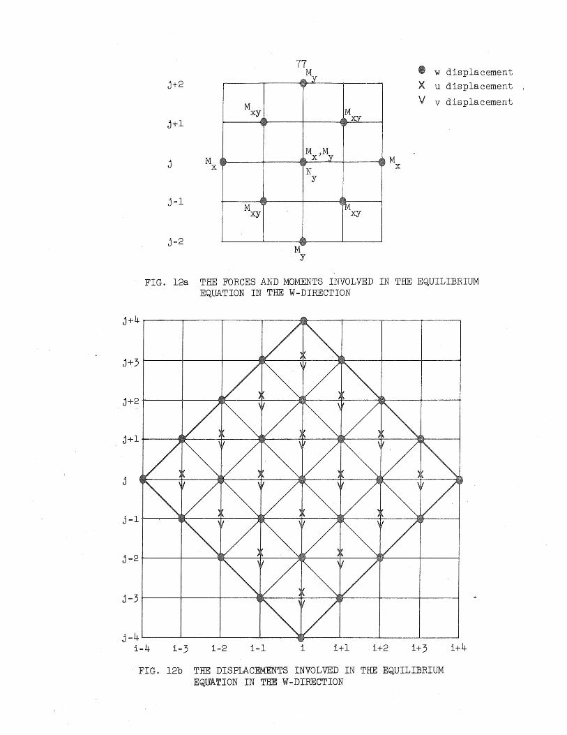
j+2
j+l
j
j-l
j-2
M x
M xy
.fill
M xy
77 M
lilA Y ".
MXJMy
N
41 II!. IT
M Y
Y
Mx:v !II'
II'
"lIlMXY
M x
• w displacement
X u displacement ,
V v displacement
FIG. l2a THE FDRCES AND MOMENTS INVOLVED IN THE EQUILIBRIUM EQUATION IN THE W-DIRECTION
j+4.-----r-----~----~----~----_T----~----~~--~
j+3
j+2~----+-----~----~----~.---~~--~~----~----~
j+l~----~----~----~~--~~--~ __ ----~----~----~
j
j-lr-~~------~----~----~----~----~~--~~--~
j-2~----~--~ __ --~~--~~----~----~----4_--~
j-3r-----~----+-----~----~----~-----+----~----~
j-4~--~----~----~--~~--~-----L----~--~
i-4 i-3 i-2 i-I i 1+1 i+2 1+3
FIG. 12b THE DISPLACEMENTS INVOLVED IN THE EQUILIBRIUM EQUATION IN THE W-DlRECTION
1+4

FIG. 13 DETAIL OF MODEL AT A FREE, EDGE
8:i+2j
~
~i+1j
FIG. 14 EQUILIBRIUM OF A T-SECTION AT A FREE EDGE

79
v .. 1 lJ-
~ v .. 1 tan 2 lJ-
t cos f312
t
2 cos)'
Displacement
ij-2
FIG. 15 JUNCTION GEOMETRY AND DISPLACEMENT CONFIGURATION OF TRANSVERSELY CONTINUOUS SHELL
t t cos (312
e .. 1 = L1 r 101 ij - 101 - v.. 1 (tan)' - tan 13/2)l YlJ - Y Lcos)'a ij -2 lJ - j
FIG. 16 MODIFIED JUNCTION GEOMETRY OF TRANSVERSELY CONTINUOUS SHELL AT NODES ONE-HALF SPACING FROM VALLEY
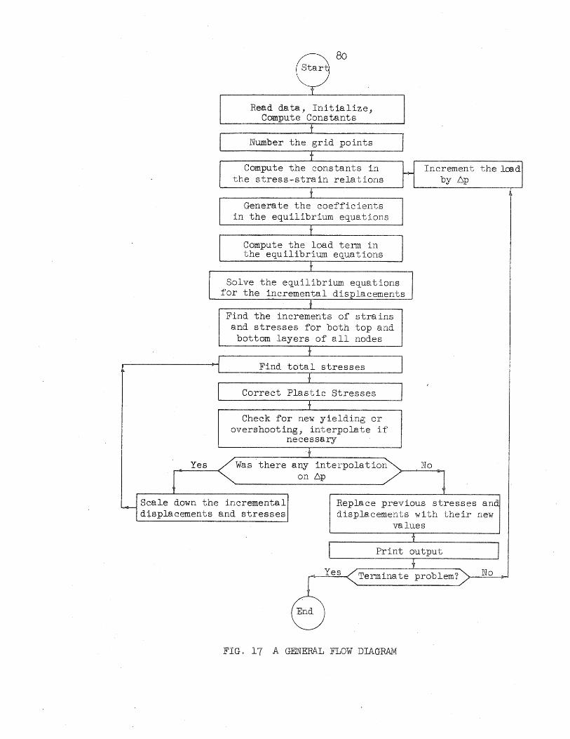
e 8 0
Read data, Initialize, Compute Constants
t Number the grid points
t Compute the constants in
~ Increment the lead
the stress-strain relations by 6p
t Generate the coefficients
in th~ equilibrium equations
t Compute the load term in the equilibrium equations
t Solve the equilibrium equations
for the incremental displacements t
Find the increments of stra ins and stresses for both top and
bottom layers of all nodes
+ Find total stresses
t I
Correct Plastic Stresses t
Check for new yielding or overshooting, interpolate if
necessa.ry
t Yes Was there any interpola.tion No
! on 6p ! Scale down the - incremental Replace previous stresses and displacements and stresses displacements with their new
values t
Print output 1
Yes Terminate problem? No
End
FIG. 1 7 A GENERAL FLOW DIAGRAM
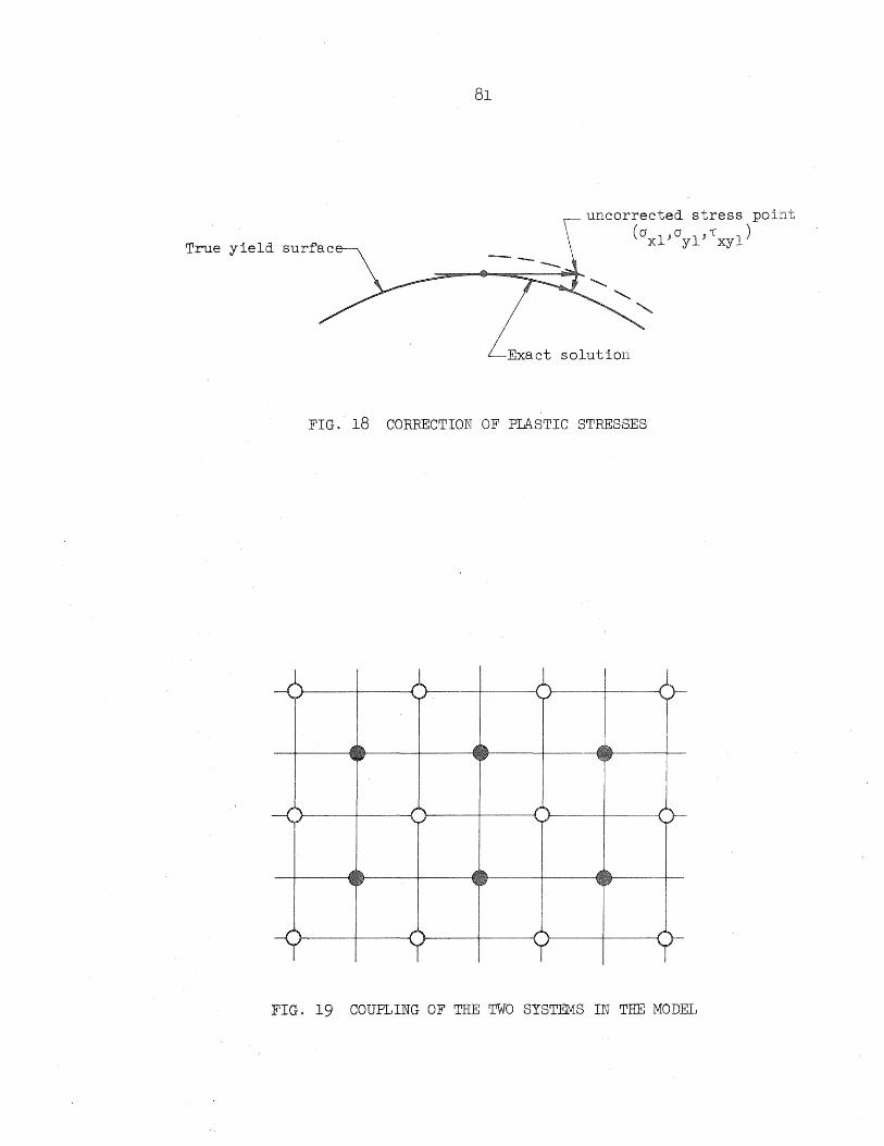
81
uncorrected stress point ( 0' 0' '[ )
xl' yl' xyl True yield sur~ac
~Exact solution
FIG. 18 CORRECTION OF PLASTIC STRESSES
FIG. 19 COUPLING OF THE TWO SYSTEMS IN THE MODEL

82
FIG. 20 SIMPLY SUPPORTED CYLINDRICAL SHELL WITH THE LONGITUDINAL EDGES FREE

I , -+- ,
I
------+-I
p = 165.9 lb/ft2
I , -+- ~
Top Layer
I
-+- , Bottom Layer
p = 222.9 lb/ft2
,-+- I
p = 229.8 lb/ft2
()) \>!
FIG. 2lil PROGRESSION OF YIELDING FOR THE CYL~NDRlCAL SHELL WITH THE FREE LONGITUDINAL EDGES

C' T~TJ d::::::::>
----- -- ---t- -
'-
p
(" ~-:r-~
I
I
.~.-.---.-.-~
f
234.0 1b/ft2
J
----~.--
'-
Top Layer
I
~:;~; j.r:g -- (;D;:~;::::;; =
Bottom Layer
p = 248.9 1b/ft2 p 263.1 1b/ft
2
FIG. 21a (cant I d) PROGRESSION OF YIELDING FOR THE CYLINDRICAL SHELL WITH THE FREE LONGITUDINAL EDGES
CX> +

D Yielded Areas
/ ......... \ I I Unloading Areas \- .....
Top layer
Bottom Layer
p = 270.3 lb/ft2
FIG. 21b FINAL STATE OF YIELDING FOR THE CYLINDRICAL SHELL SHOWN IN FIG. 20

I 260
240
220
200
180
160
140
120
100
80
60
40
20
p Ib/ft2
p = 263.5 Ib/ft2 __ = ~70·3 Ib/ft2
S.s.
= 118.4. Ib/ft2
100
Free
ree
2 I-V Q =Eh
FIG. 22 LOAD-DEFLEGTION CURVE FOR THE CENTER OF THE FREE EDGE AND A POINT HALF A SPACE FROM IT
S.S ao X
co 0\
~ x 106

free
2 l-v Q = -Eh
-100
100
00
00
400
~ x 106
FIG. 23 THE DISPIACEMENT w AT THE MIDSPAN SECTION OF THE CYLINDRICAL SHELL WITH THE FREE LONGITUDINAL EDGES
= 118~ 4 Ib/tt2
p = 22535 Ib/ft2
= 26,3.5 Ib/tt2
= 270.3 Ib/ft2
0> -.l.
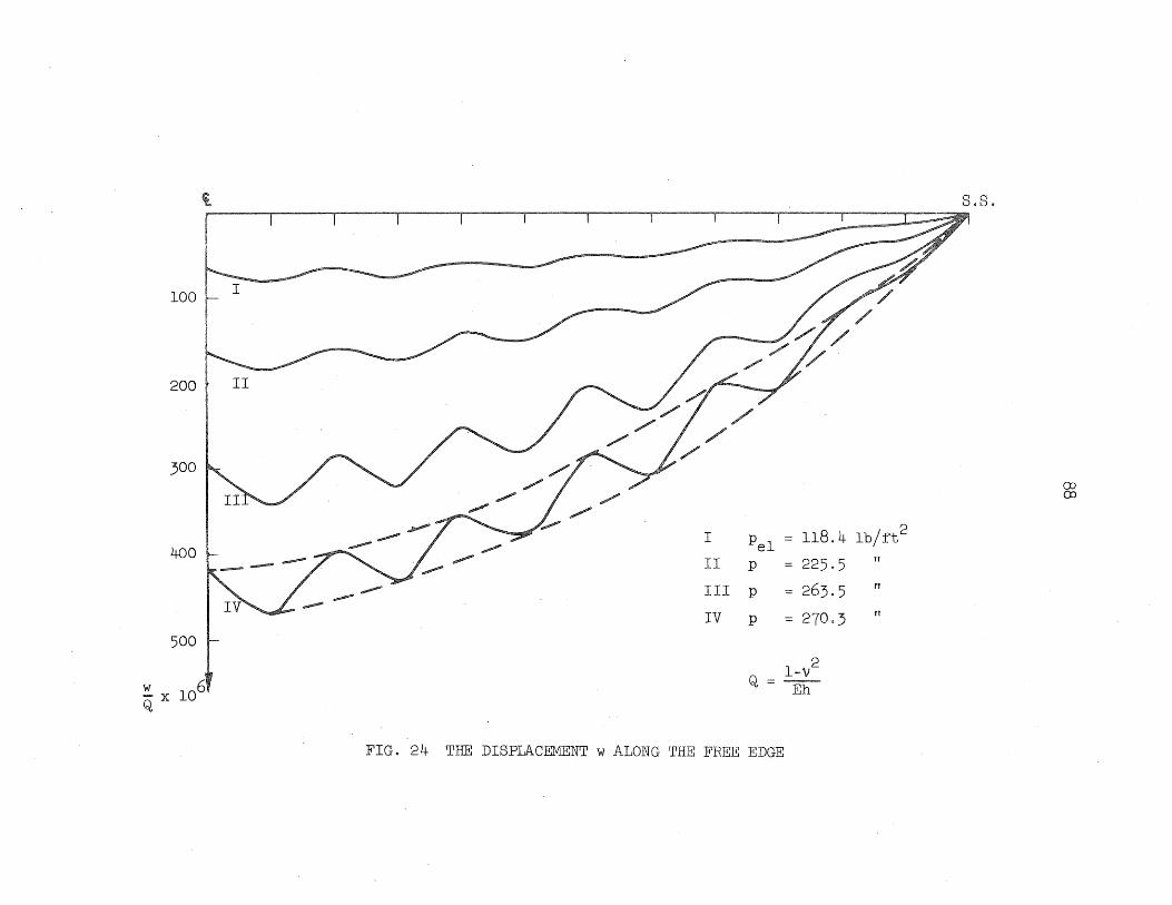
i
100 I
200 II
300
400
500
~ x 106
I Pel =: 118.4 lb/ft2
II p =: 225.5 II
III P =: 263.5 n
IV P =: 270·3 n
2 l-V Q =:--
Eh
FIG. 24 THE DISPLACEMENT w ALONG THE FREE EDGE
8.S.
OJ OJ

100
200
300
400
500
~ x 106
Free
I
II
~ __ ~==::t==~~---.-J s. s,
I
II
III
IV
2 Pel = 118.4 Ib/ft
P = 225.5 Ib/ft2
P = 263.5 lb/ft2
P = 270.3 Ib/ft2
2 I-v Q=~
y
FIG. 25 THE DISPLACEMENT w ALONG A LINE EXTENDING FROM THE FREE EDGE TO THE SIMPLY SUPPORTED EDGE
Free
S S.
x
CD '-0

y
Free
- 80 ~-~ s.s.
- 60 O\\! ~x
-40
-20
20
~ Crown
I 40 l- II
60 ~ III
IV 80
100
120
Pel = 118.4 lb/ft2
P = 225·5 fI
P = 263.5 n
P = 270·3 If
IV \
\ \ \ \ \
Crown
" ~ ~ :>tt
N x 103 ' lb/ft x
FIG. 26 VARIATION OF THE N FORCE AT MIDSPAN SECTION IN THE CYLINDRICAL SHELL WITH x
FREE LONGITUDINAL EDGES
Free
'8

<t
20
40
60
80
100
120
N x 103 J lb/ft x
Y Free --s.s.
s.s.
I
II
III
I P 1 = 118.4 1b/ft2
e 2 II P = 225.5 lb/ft
III p = 270.3 lb/ft2
FIG. 27 VARIATION OF TEE N FDRCE ALONG THE FREE EDGE x
x
\0 I-'

N x 103~ lb/ft xy
-70
-60
-50
-40
-30
-20
-10 ~~~~
~~-
y
I p 1 = 118.4 lb/ft2
e 2 II P = 225.5 lb/ft
I')
III P = 270.3 lb/ftC
,/'/
.----~ ~~
FIG. 28 VARIATION OF THE N FORCE ALONG THE SIMPLY SUPPORTED EDGE xy
Free
8.S.
n~ X
\() f\)
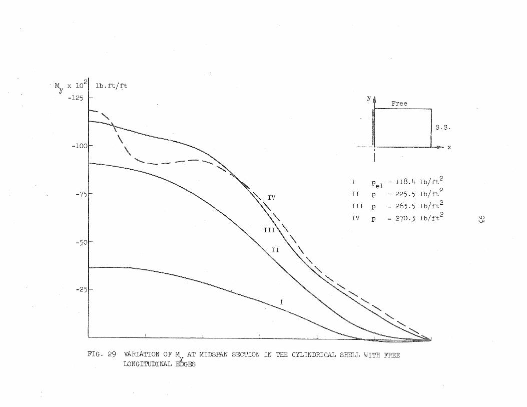
My x 102
1 1b.ft/ft
-125
-100
-75
-50
-25
y Free
S.So
~ x
I P .1 = 118.4 Ib/ft2
e 2 II p = 225.5 1b/ft
III p = 263.5 Ib/ft2
2 IV P = 270.3 Ib/ft
FIG. 29 VARIATION OF M AT MIDSPAN SECTION IN THE CYLINDRICAL SHELL WITH FREE LONGITUDINAL EbGES
\.0 \>J

-30
-20
-10
Crown
10
20
30
40
50
60
70
80
90
100
110
120
N x 10 1b/ft x
FIG. 30
94 Manua131 ------
8x8 -----.... 6 x 6
Free
COMPARISON OF THE N FORCE DISTRIBUTION AT MID SECTION x AS DETERMINED BY THE MODEL AND BY MANUAL 31

I I
I -+- +- , Top Layer
I
I.
i
\0 VI
+- ~ + -+~ I
Bottom Layer
p = 240.8 1b/tt2 p = 353.4 1b!tt2
p = 401.0 1b/tt2
FIG. 31 PROGRESSION OF YIELDING FOR A CYLINDRICAL SHELL CONTINUOUS IN THE TRANSVERSE DIRECTION
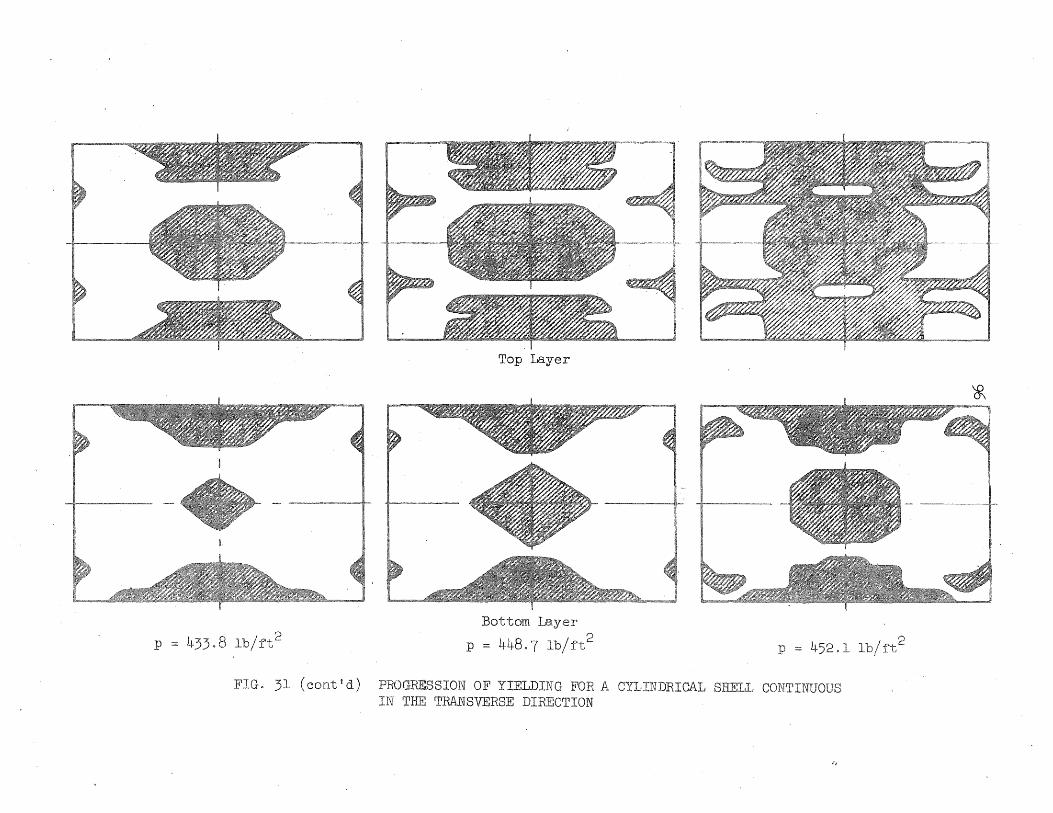
p
Top Layer
Bottom
p == 448·7 .1
FIG. ~1 (conttd) PROGRESSION OF YIELDING FOR A CYLINDRICAL SHELL CONTINlTOUS IN THE TRANSVERSE DIRECTION
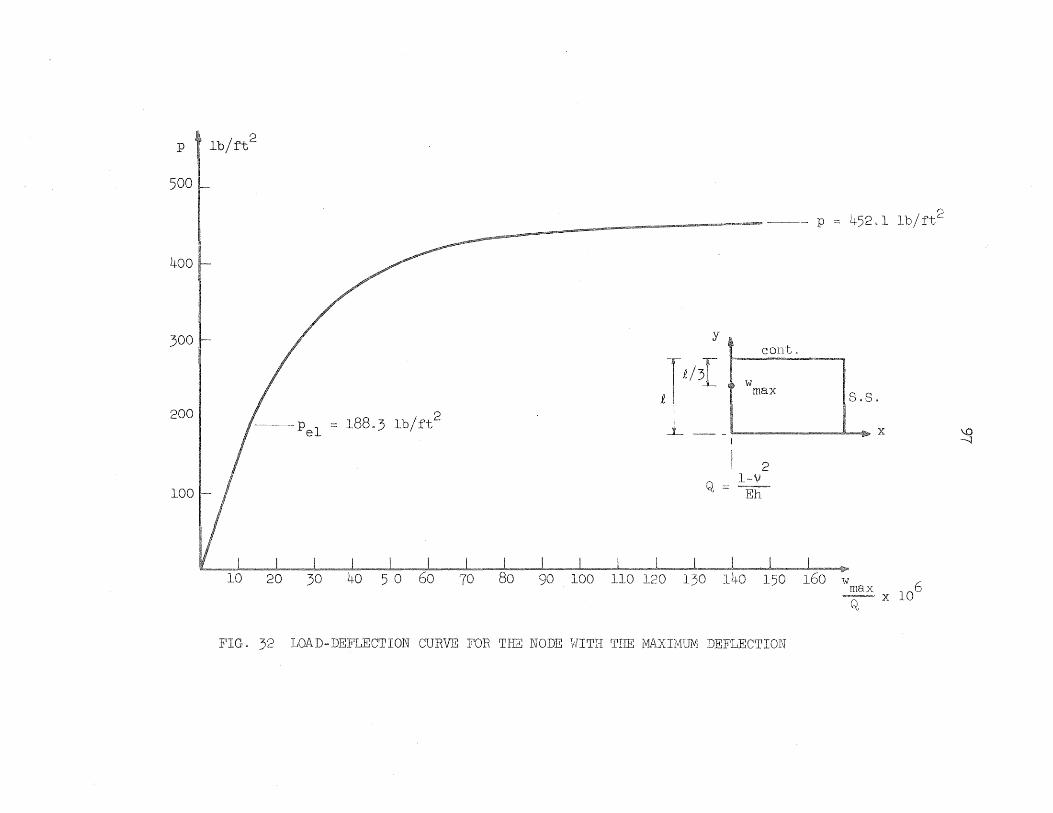
P I lb/ft2
500
400
.300
:200 188 3 lb/ft
2
100
~------------ --- p
y cant.
w max
452.1 1b/ft2
s.s.
b !tit X
2 Q :::: l-·V
x 106
FIG, ":)2 LOAD-DEFLECTION CURVE FOR THE NODE \lJITH THE MAX IlV11JIVl DEFLECTION
\0 -...;:j

cant.
10
20
30
40
50
60
70
80
90
100
110
120
130
140
~ x 106 Q
2 I-v Q = Ell
crown cont.
I
II
Pel p
III P
IV P
FIG. 33 THE DISPLAC:EMENT w AT MIDSPAN SECTION FOR THE MUIJTIPLE BARREL SHELL
= 188.3 1b/ft2
= 412.8 Ib/ft2
444.8 1b/ft2
= 452.1 1b/ft2
\0 CD

8.8. ~~
10 . I
20
30
4Dl II //r p = 188.3 lb/ ft2
II P = 412.8 lb/ft2
50 t- ~ /' III' P = 444.8 1b/ft2
60 IV P = 452.1.1b/rt2
70 \0 \0
80
I / y
90
lOO~ 110 x
l-v 2
Q=-
~ x 106 Eh
Q
FIG. 34 THE DISPLACEMENT w ALONG THE VALLEY

cant. S.S.
10~----~--'--~ ____________ --------
20
30
40
50
60
70
80
90
100
110
~ x 106
II
2 Q == l:L
Eh
I P = 188.3 lb/ft 2
o II P = 412.8 lb/ft~
III p = 452.1 lb/ft2
y
S.S.
=w .,.. X
FIG. 35 THE DISPLACEMENT w ALONG A LINE EXTENDING FROM THE CONTINUOUS EDGE TO THE SIMPLY SUPPORTED EDGE
f--' o o

/
III y
-120 ~_~IBIII_~~ cont.
II
-100
-80
-60
-40 t= I
-20
crown
20l 2
I p= 188.3 lb/ft
40 ~ II p = L~12.8 lb/ft 2
III p = 1.~52.1 lb/ft2
60 "
80
100 I " "'-
~~--~~ 120
N x 103 , 1b/ft x
FIG. 36 VARIATION OF THE N FORCE A~l MIDSPAN SECTION IN THE MULTIPLE BARREt SHELL
S.S,
IIIrX
cont.
f-' o f-'

20
40
60
80
100
120
Yf cont.
8.8.
!L. II X
r-------------~------------~--------------~------------~----....---------~------------2*~s.s.
--------~
I p:= 188. 3 Ib / ft 2
2 II p:= 412.8 Ib/ft
III p = 452.1 Ib/ft2
N x 103 If Ib/ft
x
FIG. 37 VARIATION OF THE N FORCE ALONG THE VALLEY OF THE MULTIPLE BARREL SHELL x
I--' o I'D

. 2 I P = 188.3 1b/ft
II p = 412.8 1b/ft2
III p = 452.1 1b/ft2
----------"""'""... -.......
y cont.
FIG. 38 VARIATION OF THE N FORCE ALONG THE SIMPLY SUPPORTED EDGE OF THE MULTIPLE BARREL SHELL xy
S.S.
U &J X
cant.
f-' o
\..N

-120
-100
-80
·-60
-40
-20 r----L
crown
20
40
60
80
100
120
M x 102
1 lb.ft/ft Y
I P = 188.3 lb/ft2
II p = 412.8 lb/ft2
III p = 452.1 lb/ft2
y cant.
s.S.
-, Ii\!P X
FIG. 39 'VARIATION OF AT MIDSPAN SECTION IN THE Mt~TIPLE BARREL SHELL
f-' o +:-

APPENDIX A
STRESS-DISPLACEMENT OPERATORS
The stresses in the top and bottom layers of a typical
interior node are shown here in their operator form in terms of the
displacements in Figs. A-l through A-6:
105

cT t/2L
2 11 x
.... ....
106
, -Ci1/Lx _,.,T t/L 2 , ,v11 x
\~ T T t 1 -C13 t -C12(2 + R")
L (1 + 2R) L x Y
FIG. A-I OPERATOR FOR aT x
• w-displacement
Xu-displacement
V v-displacement
,Ci1/L .. " x
CT
t/2L2
11 x"" \11 T ""
C13 t ~(1 + 2R)
x

107
4 - 12 Y
B C12 t
C~3t/LXLy _~L (1 - 2R') -y
~IP
'f-CB /1 13 Y
_CB t/2L2 -C~I/Lx CB t/L2 , "" 11 x J 11 x '" \:1
_CB Btl C12 (""2 - R) .:l2 (1 _ :L). L L 2R Y x
'11 -C~3/L -C~3t/L 1
'i' Y \ B . x y -C12 I - ~) -- ,I
L 2R Y
~_CB t 2L2 12 / y
FIG. A-2 OPERATOR FOR erE . x
..
• v-displacement
)( u-displacement
V v-diSlplacement
. B / -C13t LxLy
~~ C~l/Lx B / 2 -ClI t 2~x
,1/ B .-...
c 13 (1 _ ~) L 2R x
1
C~3t/1XLy

T / -C23t/LxLy
CT t/2L2 , .. C~l/Lx .... 21 x ; ..,
" T -C23 · t
(1 + -). L 2R x
,T / C23t LxLy
FIG. A-3
108
T 2 4 C22t/2Ly
T C22 t
wL (1 + 2R) y
,if
I CT /L 23 Y
_CT t/L2 21 x Ttl
-C22 (2" + R") L Y
T /T ~ -C23 Wy J
'_CT t 22
(1 + 2R) L Y
m 1""\
• CJ. t/2Lt::. 22 Y
• w-displacement
Xu-displacement
V v-displacement
C~3t/LXLy
I('1T /L 1~21 x CT t/2L2
21 x"", \V T
...,
C23 t L (1 + 2R)
x
-C~3t/LXLy

_CB t/2L2 SA 21 x ....
109
4 -C22t 2L Y
B / 2
B
B C22 t
\V L (1 - 2R) C23t/LxLy y 'If B Pf' C /1
23 Y
'~ -C~l/Lx CB t/12 21 x
'V B -C23
L x
B -c tiL T, 23 I x-y
Btl t C22(2 - p:)
(1 - -) 1 2R y
) -C~3/Ly \ _CB
22 (1 _ ~) L 2R
Y
E _CB t/2L2 22 Y
FIG. A-4 OPERATOR FOR crB y
/I w-displa.cement
Xu-displacement
V v-displacement
B -C23t/LX1y
..
)~C~l/Lx B / 2 -C21 t 21.,J(
W B t -C23 (1 - 2R)
C~3t/LXLy

-C~3t/LXLy
CT t/2L 2 31 x - ) -C~l/Lx
'IQIJIf
II
_CT
:lL (1 + ~). L 2R x
T C33t/LXLy
110
C C32
t 2L Y
T / 2
T C32 t
,~ L (1 + 2R) -y
,II T I
C33/Ly
_CT t/L2 31 x
Ttl -C32 ('2 + R')
L Y
T ) -C33/Ly
\ T -C32 t L (1 + 2R) y .
m 1"'\
I C.l.. t/2Lc::. • 32 y
T OPEPATOR roR 1" x::I
"
• w-displacement Xu-displacement
V v-displa cement
C~3t/LXLy
)" c~l/Lx CT t/2L2 31 Y_ -\iI T
C33 t 1" (1 + 2R)
x
-C~3t/LXLy

B , -C31/L .~ x
'V :B -c ~ (1
L x
III
t - 2R) .
\ _CB
~ (1 - !...) L 2R
Y
FIG. A-6 OPERATOR FOR ",B xy
• w-displacement
Xu-displacement
V v-disp18cement
W B -
~ t L (1 - 2R')
x
APPENDIX B
BORCE-DISPLACEMENT OPERATORS
The forces and moments similar to the finite difference form
developed about the middle surface of a real continuous shell are
obtained by combining the stresses in the top and bottom layers of
a node according to Eqs. (3.19). The operators for all the three
forces and three moments are shown below in terms of the displacements
in Figs. B-1 through B-6. In what follows A stands for (CT + CB) and
B stands for (CT _ CB).
112

-B13t / LXLy
2 Bllt/2Lx .... .....
B13t / LxLy
113
~P B12t 2L Y
/ 2
A12/Ly
II/ + B12t/2RLy
'v / 'f" Al3 Ly
~ -All/Lx 2
-Bllt/Lx ,~
-AI3/Lx 2 -BI2t/Ly
-BI3t / 2RLx -AI2/R
\., -Arz,/L
• w-disp1acement
Xu-displacement
V v-displacement
BI3t / LXLy
\~AII/L 11\ x
Bllt/2L
\V
A13/Lx
+BI3t / 2RLx
'po. ./ Y • &
,If -A /L· 12 Y
-B12t/2RLy
FIG. B-1 OPERATOR TO BE USED WITH N x
-BI3t / LXLy
2 ~ """

-B23t / LXLy
2 _B21 t/2Lx .....
B23t / LXLy
114
/ 2 ~ B22t 2Ly
A22/Ly
'v +B22t/2RLy
~ B23/Ly
• w-displacem.ent X u-disp,lacement
V v-displacement
B23t / LXLy
,11 -A21/L Ji' x -B21t/L~ yA21/Lx B21t/2L~ '~-A /L -B22t/L;
\of A23/Lx 23 x
-B23t / 2RLx -A22/R
'~23/Ly , -A /L >
22 Y
-B22t/2RLy
~B t 2L2 22 / y
FIG. B-2 OPERATOR TO BE USED WITH N Y
+B23t / 2RLx
-B23t / LXLy
...,.

115
• B32t 2L Y
/ 2
\
A32/Ly
-B33 t/LxL; 'W+B32t/2RLy \~
"" B31 t/2L;
B33t / LXLy
'f\A /L 33 y
,If -A~l /Lv , ..,...n. =B31t/ L;
'V -A /1 33 x -B32t/1;
-B33t / 2RLx -A32/R
,v-A33
/1 'I' Y \V-A32/Ly
-B_~t/2RL )!:: r y
FIG. B-3 OPERATOR TO BE USED WITH N Xl
• w-dispLacement Xu-displacement V v-displacement
B33t / LXLy
v A-z., /1 B~lt/2L i )...L. X )..L. ,;.:
2
,.,. v
A33/Lx
+B33t / 2RLx
-B33t / LXLy

All t/2L2
.... x "'"
116
• A t/2L2
• 12 Y
, w-displacement
Xu-displacement V v-displacement
) -Bll/Lx -All tiL; \ Bll/L ,I>. X All t/2L 2
~
"-B /L 13 x -A12t/L~
-A13t / 2RLx -B12/R
FIG. B ... 4 OPERATOR TO BE USED WITH M x
.., vB /1
13 x
+A13t / 2RLx

L ht x
117
=-8- [ J
-.A21 t/2L; ..,
/ 2 4 A22t 2L Y
B22/Ly i
-A 23t/LXLy V +A22t/2RLy
) B /L 23 Y
, -B21/Lx -A21 tiL; , 'II
-B23/Lx -A22t/L~
A23t / LXLy
--A23t / 2RLX -B22/R
,~-B23/L Jr,. Y
\~-B /L ' 22 Y
-A22t/2RLy
C A22t/2L2 y
FIG. B-5 OPERATOR TO BE USED WITH M Y
• v-displacement X u-d1spla cement V v-displacement
A23t / LXLy
,~ B21/L i~ x
A21t/2L; ""'"
,~ "'"'
B23/Lx
+A23t / 2RLx
..
-A 23t/LXLy
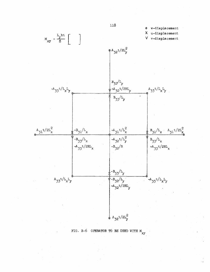
A31t/2L~
118
=+ [ ] • w-d1splacement X u-d1splacement
V v-displa.cement
+A;2t/2RLy A;3t / LXLy ~~--~~~---+---=--~------4
=B;l/Lx
=B;;/LX
...A.;3t/2RLX
B33/Ly
-A;l tiL;
-A;2t / L;
-B32/R
=B3JLy -
-A32t/2RLy
FIG. B-6 OPERATOR TO BE OSED WITH
B31/Lx ' A;l t/2L;
B;;/LX
+A;3t / 2RLx