a backward–forward regularization of the perona–malik …gpatrick/source/papers/g121.pdf ·...

J. Differential Equations 252 (2012) 3226–3244

Contents lists available at SciVerse ScienceDirect

Journal of Differential Equations

www.elsevier.com/locate/jde

A backward–forward regularization of the Perona–Malikequation

Patrick Guidotti

Department of Mathematics, 340 Rowland Hall, University of California at Irvine, Irvine, CA 92697-3875, United States

a r t i c l e i n f o a b s t r a c t

Article history:Received 18 February 2011Revised 28 October 2011Available online 6 December 2011

Keywords:Nonlinear diffusionForward–backward diffusionWell-posednessYoung measure solutionsPerona–Malik type equationGlobal existenceQualitative behavior

It is shown that the Perona–Malik equation (PME) admits a natu-ral regularization by forward–backward diffusions possessing bet-ter analytical properties than PME itself. Well-posedness of theregularizing problem along with a complete understanding of itslong time behavior can be obtained by resorting to weak Youngmeasure valued solutions in the spirit of Kinderlehrer and Pe-dregal (1992) [1] and Demoulini (1996) [2]. Solutions are unique(to an extent to be specified) but can exhibit “micro-oscillations”(in the sense of minimizing sequences and in the spirit of ma-terial science) between “preferred” gradient states. In the limit ofvanishing regularization, the preferred gradients have size 0 or ∞thus explaining the well-known phenomenon of staircasing. Thetheoretical results do completely confirm and/or predict numericalobservations concerning the generic behavior of solutions.

© 2011 Elsevier Inc. All rights reserved.

1. Introduction

Ever since it was proposed by Perona and Malik in 1990 [3], the so-called Perona–Malik equation(PME)

ut = ∇ ·(

1

1 + |∇u|2 ∇u

)=: ∇ · (a

(|∇u|2)∇u)

(1.1)

E-mail address: [email protected]: http://www.math.uci.edu/~gpatrick.

0022-0396/$ – see front matter © 2011 Elsevier Inc. All rights reserved.doi:10.1016/j.jde.2011.10.022

http://dx.doi.org/10.1016/j.jde.2011.10.022

http://www.ScienceDirect.com/

http://www.elsevier.com/locate/jde

mailto:[email protected]

http://www.math.uci.edu/~gpatrick

http://dx.doi.org/10.1016/j.jde.2011.10.022

P. Guidotti / J. Differential Equations 252 (2012) 3226–3244 3227

has attracted the interest of the mathematical community. It is an example of a nonlinear forward–backward heat equation which is not (directly) amenable to variational techniques. It is in fact theformal gradient flow generated by the convex-concave energy functional

E(u) = 1

2

∫Ω

log(1 + |∇u|2)dx =

∫Ω

ϕ(|∇u|)dx. (1.2)

The arguably most natural variational approach to understand and solve this problem does not seemviable as the relaxation of the energy functional (1.2) vanishes everywhere; indeed ϕ ≡ 0 for theconvexification ϕ of ϕ . In an effort to overcome this difficulty Zhang and co-authors [4] and [5] in-troduced an ad-hoc concept of weak Young measure valued solution for (1.1) in one space dimensionby rewriting the equation as a first order system. They proved existence of infinitely many such so-lutions (non-uniqueness) and obtained instability results. The class of solutions they consider excludeclassical solutions. In this regard we observe that (1.1) does admit global in time classical solutionsin the subcritical region where |∇u| < 1 which, as it turns out [6], is invariant under the evolution.In other words subcritical initial data yield classical solutions which remain subcritical for all timesand converge to trivial (constant) steady-states. Such solutions cannot be captured by variational re-laxation techniques which, as pointed out above, deliver a vanishing convexification and no evolutionwhatsoever for any initial datum. More recently, Smarrazzo and Tesei [7–9] obtained some general,albeit one-dimensional, results for forward–backward equations of PME type (not including PME) inthe vanishing limit of a degenerate pseudo-parabolic regularization à la [10]. They use the concept ofYoung measure valued solution (different from the above one employed by Zhang), follow some ideasand techniques of [11–13] which rely on entropy inequalities. Many other regularization approacheswere previously proposed over the years, starting with the early [14] up to the more recent [15–17],and through [18–25] to mention just a few. Other authors have obtained results concerning certainclasses of classical solutions and/or their qualitative properties starting with [26], where ill-posednessin the one-dimensional setting is proved, and followed by [6,27–30]. Ghisi and Gobbino recently con-structed an interesting family of global classical solutions of PME to transcritical initial conditions intwo space dimensions. Finally there exist attempts at obtaining insights concerning the behavior ofsolutions to PME by semi-discretizations in space [31–33]. Many of the efforts mentioned were mo-tivated by the desire to reconcile empirical, numerical observations about the behavior of solutionsto PME with its mathematical properties so as to provide satisfactory theoretical explanations forthem.

Here another, and arguably quite natural, approach is proposed by which the equation is verymildly regularized by a family of better natured forward–backward equations and which works inany space dimension. This novel regularization is even milder than that proposed in [15] but has theadvantage of having a variational structure. The latter allows for an analysis based on general resultsoutlined in [1] and obtained by Demoulini in [2]. The regularization simply reads

ut = ∇ ·([

1

1 + |∇u|2 + δ

]∇u

)=: ∇ · (aδ

(|∇u|2)∇u)

(1.3)

=: ∇ · (qδ(∇u)). (1.4)

While 0 < δ � aδ � 1 + δ holds for the regularized problem (1.3), which makes the problem uniformlyparabolic, it remains of forward–backward type for δ < 1/8 and, thus, in the small δ regime of interest.The energy functional (1.2) is only mildly concave so that any δ > 0 is enough to make

Eδ(u) = 1

2

∫ {log

(1 + |∇u|2) + δ|∇u|2}dx =:

∫ϕδ(∇u)dx (1.5)

Ω Ω

3228 P. Guidotti / J. Differential Equations 252 (2012) 3226–3244

Fig. 1. The potential ϕδ for δ = 0,0.01,0.03 (solid, dashed, and dotted line, respectively).

Fig. 2. The driving function aδ(s2)s for δ = 0,0.01,0.03 (solid, dashed, and dotted line, respectively).

eventually convex. See Fig. 1. The original convex-concave energy E (1.2) is turned into the convex-concave-convex energy Eδ . To be more precise (1.3) can be rewritten as

ut = aδ

(|∇u|2)�u + 2a′δ

(|∇u|2)∇uT D2u∇u

= aδ

(|∇u|2)∂ττ u + {aδ

(|∇u|2) + 2a′δ

(|∇u|2)|∇u|2}∂ννu (1.6)

by means of local coordinates in tangential τ and normal direction ν to the level sets of u. Dependingon the size of |∇u| diffusion in normal direction can still be backward. It is now, however, forwardfor |∇u| � 1 and for |∇u| � 1√

δfor δ ≈ 0. This behavior can be read off Fig. 2. The regions where the

function aδ(s2)s is increasing and decreasing correspond to those where the equation is forward and


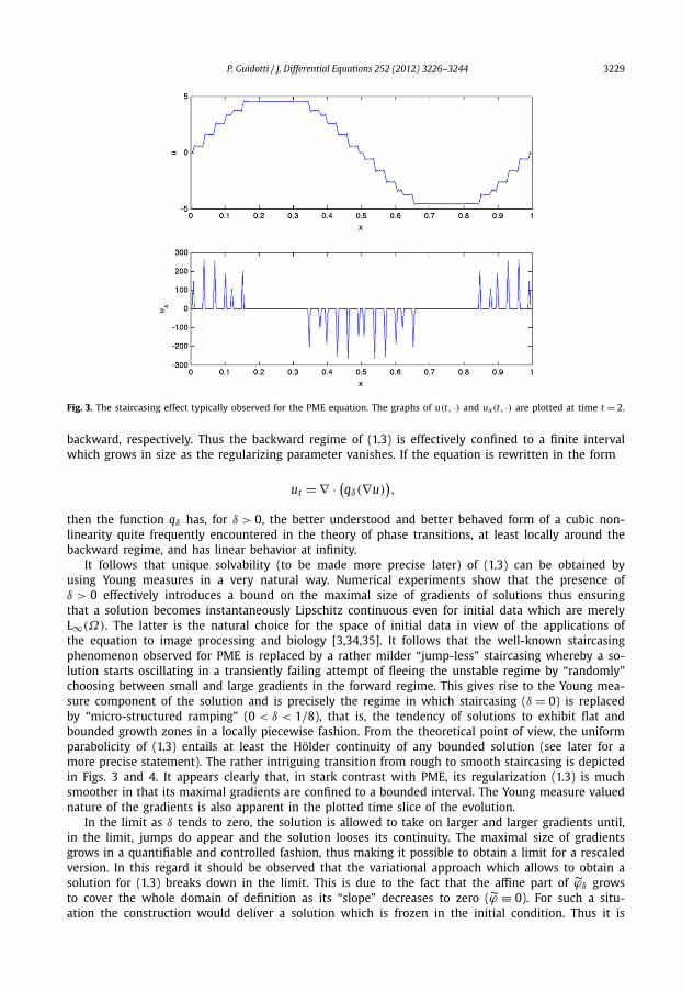
Fig. 3. The staircasing effect typically observed for the PME equation. The graphs of u(t, ·) and ux(t, ·) are plotted at time t = 2.

backward, respectively. Thus the backward regime of (1.3) is effectively confined to a finite intervalwhich grows in size as the regularizing parameter vanishes. If the equation is rewritten in the form

ut = ∇ · (qδ(∇u)),

then the function qδ has, for δ > 0, the better understood and better behaved form of a cubic non-linearity quite frequently encountered in the theory of phase transitions, at least locally around thebackward regime, and has linear behavior at infinity.

It follows that unique solvability (to be made more precise later) of (1.3) can be obtained byusing Young measures in a very natural way. Numerical experiments show that the presence ofδ > 0 effectively introduces a bound on the maximal size of gradients of solutions thus ensuringthat a solution becomes instantaneously Lipschitz continuous even for initial data which are merelyL∞(Ω). The latter is the natural choice for the space of initial data in view of the applications ofthe equation to image processing and biology [3,34,35]. It follows that the well-known staircasingphenomenon observed for PME is replaced by a rather milder “jump-less” staircasing whereby a so-lution starts oscillating in a transiently failing attempt of fleeing the unstable regime by “randomly”choosing between small and large gradients in the forward regime. This gives rise to the Young mea-sure component of the solution and is precisely the regime in which staircasing (δ = 0) is replacedby “micro-structured ramping” (0 < δ < 1/8), that is, the tendency of solutions to exhibit flat andbounded growth zones in a locally piecewise fashion. From the theoretical point of view, the uniformparabolicity of (1.3) entails at least the Hölder continuity of any bounded solution (see later for amore precise statement). The rather intriguing transition from rough to smooth staircasing is depictedin Figs. 3 and 4. It appears clearly that, in stark contrast with PME, its regularization (1.3) is muchsmoother in that its maximal gradients are confined to a bounded interval. The Young measure valuednature of the gradients is also apparent in the plotted time slice of the evolution.

In the limit as δ tends to zero, the solution is allowed to take on larger and larger gradients until,in the limit, jumps do appear and the solution looses its continuity. The maximal size of gradientsgrows in a quantifiable and controlled fashion, thus making it possible to obtain a limit for a rescaledversion. In this regard it should be observed that the variational approach which allows to obtain asolution for (1.3) breaks down in the limit. This is due to the fact that the affine part of ϕδ growsto cover the whole domain of definition as its “slope” decreases to zero (ϕ ≡ 0). For such a situ-ation the construction would deliver a solution which is frozen in the initial condition. Thus it is


Fig. 4. The “gentler” staircasing effect observed for equation (1.3) for δ = 0.001. The dotted lines correspond to approximatedgradient values at which the transition between forward and backward regime occur. The graphs of u(t, ·) and ux(t, ·) areplotted at time t = 2 of the evolution.

seen again that the only way to produce a meaningful limit would involve a rescaling of time in theprocess. After receiving a preliminary version of this paper, Colombo and Gobbino were able to useGamma convergence techniques to carry out this very suggestion. Interestingly they found that care-fully rescaled families of solutions uδ do possess a limit for vanishing δ which does evolve accordingto the well-known Total Variation flow. It is referred to their paper [36] for the details.

It is worthwhile mentioning that the properties of regularization (1.3) have important conse-quences in applications to image processing. The latter will be considered in another more appliedpaper.

While the numerical observations made for the regularized problem cannot be all proven in theirstrongest form, they can certainly all be justified by the theoretical results presented here. They in-clude global existence of weak Young measure valued solutions in any space dimension which doeventually converge to trivial steady-states and which admit Young measure representations of theirgradients the support of which concentrate in the origin and at infinity in the vanishing regulariza-tion parameter limit. Young measures are well suited for capturing the oscillations in the solutions’gradient between preferred states which give rise to “micro-structured” gradients.

For the sake of completeness it should be observed that, while the class of solutions constructed inthis paper do indeed satisfactorily predict and reflect the behavior observed in numerical simulations,it does exclude certain classical solutions of the original problem. This is due to the fact that therelaxation procedure employed here does modify the original energy in its forward (convex) region aswell.

The paper is organized as follows. In the next section the Young measure valued approach to thesolvability of certain forward–backward equations is presented. In Section 3 the results are applied tothe regularized problem (1.3). The results of numerical experiments are shown all along in order tomotivate and/or underscore the theoretical findings.

2. Young measures and forward–backward diffusions

The use of non-convex functionals in the calculus of variations for applications in material sciencehas been discussed by Chipot and Kinderlehrer in [37] where they introduced a crucial stability cri-terion. Later Kinderlehrer and Pedregal [1] found sufficient conditions for the validity of the criterion


in terms of growth properties of the potential ϕ , thus ensuring the availability of important Youngmeasure representations. They also outlined applications of various nature including one to the res-olution of evolution equations. Demoulini [2] finally obtained comprehensive results about existence,uniqueness, and qualitative properties of solutions to gradient systems satisfying these conditions inthe case of homogeneous Dirichlet boundary conditions.

A description of the method is given here in which the results of Demoulini are translated from theDirichlet into the periodic and Neumann settings considered in this paper. Given a bounded domainΩ ⊂ R

N (N � 1) with piecewise smooth boundary ∂Ω , of interest is the divergence form evolutionaryequation

⎧⎪⎨⎪⎩

ut = ∇ · (q(∇u)), in Q ∞ := R

+ × Ω,

q(∇u) · ν = 0, on ∂ Q ∞ := R+ × ∂Ω,

u(0, ·) = u0, in Ω,

(2.1)

where the homogeneous Neumann conditions can be replaced by a periodicity assumption providedthe domain is set to be a unit box. The structural assumption that

q = ∇ϕ for ϕ ∈ C1(R

N)is made along with the requirement that

(c|ξ |2 − 1

)+ � ϕ(ξ) � C |ξ |2 + 1, ξ ∈ RN and (2.2)

0 � q(ξ) · ξ,∣∣q(ξ)

∣∣ � C |ξ |, ξ ∈ RN , (2.3)

for some 0 < c � C < ∞. Given a fixed but arbitrary u0 ∈ H1(Ω), the space H1u0

(Ω) will denote theaffine space of H1(Ω)-functions satisfying

∫Ω

u dx =∫Ω

u0 dx

or its subspace of periodic functions satisfying the same condition depending on the choice of bound-ary condition. It is also recalled that a Young measure on Ω × R

N is a positive measure μ such that

μ(

A × RN) = λN(A), A ∈ B

(R

N),

where B(RN ) is the collection of Borel sets of RN and λN is the N-dimensional Lebesgue measure. It

is possible to associate a Young measure to any given measurable function z : Ω → RN by setting

μz = (δz(x))x∈Ω.

The disintegration (μx)x∈Ω of a Young measure μ (which does always exist, cf. [38]) is such that forany f ∈ C(Ω × R

N ) one has

〈μ, f 〉 =∫Ω

∫RN

f (x, ξ)dμx(ξ)dx,

and thus, in particular,


〈μz, f 〉 =∫Ω

f(x, z(x)

)dx.

Finally it is said that μ is generated by a sequence of functions (zn)n∈N in L1(Ω)N whenever

∫Ω

f(x, zn(x)

)dx = 〈μzn , f 〉 → 〈μ, f 〉, f ∈ Cc

(Ω × R

N).

The point is here of course that μ does not need to be, and, in general is not, a Young measureassociated to any function. This allows the concept to capture the limiting behavior of certain increas-ingly oscillating sequences of functions (cf. [39]). Notice that the spaces H1

loc(Q ∞) and H10,loc(Q ∞) are

defined through

H1loc(Q ∞) = {

u : Q ∞ → R∣∣ u ∈ H1(Q T ) for T > 0

},

and

H10,loc(Q ∞) = {

u : Q ∞ → R∣∣ u ∈ H1(Q T ) for T > 0 and u(·, t) ∈ H1

0(Ω) a.e. in Q ∞},

respectively.

Definition 1. A weak Young measure valued solution of (2.1) is a pair (u, ν) where

u ∈ H1loc(Q ∞) ∩ L∞(

R+,H1(Ω)

)and ν = (νx,t)(x,t)∈Q ∞ is a Young measure generated by a sequence of spatial gradients (as will beexplained below) such that

∫Q T

{utψ + 〈ν,q〉∇ψ

}dx dt = 0, ψ ∈ H1(Q T ), T > 0,

and such that they are connected through

∇u(t, x) =∫

RN

ξ dνx,t(ξ) a.e. in Q ∞.

Remark 2. By inserting the constant test function ψ = 1Ω with value 1 in the above weak equation,it readily follows that the mean of any solution is a conserved quantity

d

dt

∫Ω

u dx = −∫Ω

〈ν,q〉0 dx = 0.

From now on, it will therefore be required for a solution to satisfy u(t) ∈ H1u0

(Ω) a.e. in t � 0 and

that the weak formulation be satisfied for all test functions in the subspace H10(Q ∞).


Following [1] and [2], a solution of (2.1) is obtained by semi-discretization in time and passage tothe limit. Let h > 0 and let u j,h ( j � 1) be given as the minimizer of the functional

Ehuh, j−1(v) :=

∫Ω

ϕ(∇v)dx + 1

2h

∫Ω

(v − uh, j−1)2

dx, v ∈ H1(Ω),

over v ∈ H1(Ω) where uh,0 := u0. Since ϕ is not necessarily convex, and following relaxation theory,ϕ is replaced by its convexification ϕ . The energy functional Eh has the same infimum as

Ehuh, j−1(v) :=

∫Ω

ϕ(∇v)dx + 1

2h

∫Ω

(v − uh, j−1)2

dx, v ∈ H1(Ω).

It is readily seen that

Ehu0

(v − �

∫Ω

v dx + �

∫Ω

u0 dx

)� Eh

u0(v), v ∈ H1(Ω),

and that

Ehu0

(v − �

∫Ω

v dx + �

∫Ω

u0 dx

)� Eh

u0(v), v ∈ H1(Ω).

It follows that minimizers and minimizing sequences can all be assumed to lie in H1u0

(Ω) withoutloss of generality, in keeping with Remark 2. By defining

uh : R+ → H1

u0(Ω)

on the whole positive axis by linear interpolation on the intervals [( j − 1)h, jh) using the sequence(uh, j) j∈N , and setting νh to be piecewise constant on the same intervals using the Young measure

associated with the sequence of gradients ∇uh, jn of a minimizing sequence (uh, j

n )n∈N for the corre-sponding energy functional, an approximating sequence is obtained for the solution of the continuoustime problem which satisfies the equation a.e. in time. A priori estimates are available as a conse-quence of the dissipativity of the equation reflected in

∫Ω

ϕ(∇uh, j)dx + 1

2h

∫Ω

(uh, j − uh, j−1)2

dx �∫Ω

ϕ(∇uh, j−1)dx, j � 1,

and allow for the construction of a limit. One eventually obtains a solution of the original problemas summarized in the following theorem along with some qualitative properties which are a niceconsequence of the construction. While an almost complete proof of the result will be given here, theinterested reader is referred to [2] for further details of the arguments used in it modulo, of course,the necessary changes caused by the different functional setting.

Theorem 3. Let the assumptions (2.2)–(2.3) be satisfied and take u0 ∈ H1(Ω). Then problem (2.1) possessesa unique1 weak Young measure valued solution (u, ν). Uniqueness only pertains to the function u while the

1 See Remark 4 following the proof of the theorem.


(gradient) Young measure ν = (νx,t)x,t∈Q ∞ is in general not unique. It is also the solution of the relaxed prob-lem

ut = ∇ · p(∇u),

where p = ∇ϕ . One also has that

ut ∈ L2(Q ∞),

that

supp(νx,t) ⊂ [ϕ = ϕ] ∩ A(ϕ) a.e. in Q ∞,

and that

∇u(x, t) =∫

RN

ξ dνx,t(ξ) a.e. in Q ∞.

Here A(ϕ) denotes the collection of all subsets on which ϕ behaves in an affine manner. Any solution eventuallyconverges to a Young measure valued solution (u∞, ν∞) of the corresponding stationary problem in the sensethat

u(t, ·) ⇀ u∞ in H1u0

(Ω) as t → ∞,

∇u∞ =∫

RN

ξ dν∞(ξ) a.e. in Ω, (2.4)

and it holds that

supp(ν∞) ⊂ [

ξ · q(ξ) = 0] ∩ [ϕ = ϕ = 0].

The comparison principle holds, that is,

−∥∥(u0 − v0)−∥∥∞ � u(t, x) − v(t, x) �

∥∥(u0 − v0)+∥∥∞ a.e. in Q ∞

is valid for any pair (u, ν), (v,μ) of Young measure valued solutions of (2.1) with initial data u0 and v0 ,respectively.

Proof. Let h > 0 and consider the following equation

1

h(u − w) = ∇ · p(∇u),

which can clearly be viewed as a single time step discretization of the gradient flow

ut = ∇ · p(∇u), t > 0, u(0) = w,

corresponding to the convexified problem. The idea is to construct a sequence by recursively solvingthis equation for u given w starting with w = u0 and subsequently with w = uh, j where uh, j is the


solution computed last. Since, for any given uh, j−1 ∈ H1u0

(Ω), the equations are the Euler–Lagrangeequations for the strictly convex variational problem

argmin∫Ω

{ϕ(∇v) + 1

2h

∣∣v − uh, j−1∣∣2

}dx = argmin Eh

uh, j−1(v), v ∈ H1(Ω),

this amounts to recursive minimization of the functionals Ehuh, j−1 . Now a sequence (uh, j,k)k∈N can al-

ways be chosen such that it approximates the minimum uh, j of Ehuh, j−1 and such that it simultaneously

is a minimizing sequence for

Ehuh, j−1(v) =

∫Ω

{ϕ(∇v) + 1

2h

∣∣v − uh, j−1∣∣2

}dx, v ∈ H1(Ω),

since one function is the relaxation of the other. The growth assumptions on ϕ entail that

∥∥uh, j,k∥∥

H1(Ω)� c < ∞, k ∈ N.

There exists therefore uh, j ∈ H1u0

(Ω) such that

uh, j,k ⇀ uh, j in H1u0

(Ω),

uh, j,k → uh, j in L2(Ω),

as k → ∞, by compactness of the embedding H1(Ω) ↪→ L2(Ω). Clearly

inf Ehuh, j−1 = lim

k→∞Eh

uh, j−1

(uh, j,k) = lim

k→∞Eh

uh, j−1

(uh, j,k)

= min Ehuh, j−1 = Eh

uh, j−1

(uh, j). (2.5)

Again by means of the growth assumptions on ϕ (and thus on ϕ) and using the main results of [1](also restated in the introduction of [2]) it follows that

ϕ(∇uh, j,k) ⇀ ϕ

(∇uh, j) in L1(Ω).

Denote by νh, j the Young measures generated by the sequences (∇uh, j,k)k∈N . By [2, Theorem 2.3] itis an H1(Ω)-gradient Young measure and, once more thanks to the growth assumptions on ϕ , onehas that ϕ(∇uh, j,k) is weakly convergent in L1(Ω) and, using (2.5), that

∫Ω

ϕ(∇uh, j)dx =

∫Ω

⟨νh, j, ϕ

⟩dx =

∫Ω

⟨νh, j,ϕ

⟩dx.

It should be pointed out that [1, Theorem 1.3] plays a crucial role here. Since ϕ � ϕ by definition ofconvexification, it follows that

supp(νh, j) ⊂ [ϕ = ϕ] a.e. in Ω,⟨

νh, j,ϕ⟩ = ⟨

νh, j, ϕ⟩ = ϕ

(∇uh, j) a.e. in Ω,

∇uh, j = ⟨νh, j, id

⟩a.e. in Ω.


Using [∇ϕ = ∇ϕ] ⊃ [ϕ = ϕ] one also infers that

⟨νh, j,q

⟩ = ⟨νh, j, p

⟩a.e. in Ω.

Jensen’s inequality yields

ϕ(⟨νh, j, id

⟩)�

⟨νh, j, ϕ

⟩ = ϕ(∇uh, j) = ϕ

(⟨νh, j, id

⟩)a.e. in Ω, (2.6)

which, in turn, entails that supp(νh, j) lies in a connected region where ∇ϕ is constant because equal-ity in Jensen’s inequality only holds in the affine case.

It is plain that the minimizer uh, j satisfies the corresponding Euler–Lagrange equation, i.e., that

∇ · p(∇uh, j) = 1

h

(uh, j − uh, j−1) in H−1(Ω) = H1

0(Ω)′,

or, equivalently that

⟨p(∇uh, j),∇ψ

⟩ = 1

h

⟨uh, j − uh, j−1,ψ

⟩, ψ ∈ H1

0(Ω). (2.7)

Now, using an argument of [1,37], consider

ϕ(ξ + ε∇ψ(x)

)� C

(1 + |ξ |2), ξ ∈ R

N ,

for ψ ∈ C10(Ω) := {ψ ∈ C1(Ω) | ∫

Ωψ = 0} such that |∇ψ | ∈ L∞(Ω) and for ε ∈ [−1,1]. Then

∫Ω

[⟨νh, j,ϕ

⟩ + 1

2h

(uh, j − uh, j−1)2

]dx

=∫Ω

[⟨νh, j, ϕ

⟩ + 1

2h

(uh, j − uh, j−1)2

]dx

� limk→∞

∫Ω

[⟨νh, j, ϕ

(∇uh, j,k + ε∇ψ)⟩ + 1

2h

(uh, j + εψ − uh, j−1)2

]dx

=∫Ω

[⟨νh, j, ϕ(· + ε∇ψ)

⟩ + 1

2h

(uh, j + εψ − uh, j−1)2

]dx

�∫Ω

[⟨νh, j,ϕ(· + ε∇ψ)

⟩ + 1

2h

(uh, j + εψ − uh, j−1)2

]dx

and differentiating in ε = 0 yields

−∇ · ⟨νh, j,q⟩ + 1

h

(uh, j − uh, j−1)

= −∇ · ⟨νh, j, p⟩ + 1 (

uh, j − uh, j−1) = 0 in H−1(Ω). (2.8)
h


To conclude the latter it is necessary to show that any ψ ∈ H10(Ω) can be approximated by ψε ∈ C1

0(Ω)

with ‖∇ψε‖∞ � Cε < ∞. This, however, follows from the boundedness of the Helmholtz projection

P : L2(Ω)N → L2(Ω)N , u �→ P u

in L2(Ω) onto divergence free vector fields. Consider, in fact, a cut-off function χε ∈ C∞c (Ω) and a

mollifier ϕε ∈ C∞c (Ω). Then

(1 − P )ϕε ∗ (∇ψ · χε) =: ∇ψε ∈ C∞(Ω)

for some ψε ∈ C∞(Ω) with∫Ω

ψε dx = 0. Since

ϕε ∗ (∇ψ · χε) → ∇ψ in L2(Ω),

one also has that

∇ψε → (1 − P )∇ψ = ∇ψ in L2(Ω).

By Poincaré’s inequality ‖ψ − ψε‖2 � C‖∇ψ − ∇ψε‖2 and the claim follows.Define now

uh(x, t) = uh, j(x) + (t − jh)1

h

(uh, j+1 − uh, j), x ∈ Ω,

wh(x, t) = uh, j(x), x ∈ Ω,

νh = (ν

h, jx

)x∈Ω

,

for t ∈ [ jh, ( j + 1)h), j � 0. Then

uh, wh ∈ L∞([0,∞),H1u0

(Ω)), νh ∈ L1

loc

(Q ∞, E 1

0

) ∩ L∞(Q ∞, M

(R

N))uniformly in h > 0 (in the sense that a bound exists in the corresponding norm which is independentof h > 0). Here the notation

E 10 :=

{q ∈ C

(R

N) ∣∣∣ lim|ξ |→∞|q(ξ)|

1 + |ξ | exists

}

was used following [2]. Observe that

⟨νh,q

⟩ ∈ L∞([0,∞), L2(Ω)),

and that

uht = 1

h

(uh, j+1 − uh, j) on

[jh, ( j + 1)h

).

It follows that {uht | h > 0} is bounded in L2(Q ∞) since

∞∫ ∫ ∣∣uht

∣∣2dx dt =

∑j�1

1

h

∫ (uh, j+1 − uh, j)2

dx �∫

ϕ(∇u0)dx,

0 Ω Ω Ω


where the inequality holds by construction. Given T > 0, (2.7) and (2.8) yield

T∫0

∫Ω

{⟨νh,q

⟩ · ∇ψ + uht ψ

}dx dt = 0, ψ ∈ H1

0(Q T ),

by density of tensor products ψ(x, t) = ψ1(x)ψ2(t) in H10(Q T ). Clearly one has 〈νh,q〉 = 〈νh, p〉 for

t > 0 and a.e. in Ω as well as

∇ · ⟨νh,q⟩ = ∇ · ⟨νh, p

⟩ = ∇ · p(∇uh) for t > 0 in H−1(Ω)

and in H−1(Q T ) as seen above for any T > 0. The family (νh)h>0 is uniformly bounded in

L∞([0,∞), L∞(Ω,

(E 1

0

)′)) = L1(Q ∞, E 10

)′

and (〈νh,q〉)h>0 is uniformly bounded in

L∞([0,∞), L2(Ω)) = L1([0,∞), L2(Ω)

)′.

Moreover uh and wh are uniformly bounded in

H1loc(Q ∞) ∩ L∞([0,∞),H1

u0(Ω)

).

By weak compactness a subsequence can be found, which is not relabeled, converging to (u, ν) whereu is the common limit of uh and wh in L2

loc(Q ∞) (as shown at the end of [1]). It holds that

u ∈ H1loc(Q ∞) ∩ L∞([0,∞),H1

u0(Ω)

), ut ∈ L2(Q ∞),

that, for T > 0,

T∫0

∫Ω

{〈ν,q〉 · ∇ψ + utψ}

dx dt = 0, ψ ∈ H10(Q T ),

and that

〈ν,q〉 = 〈ν, p〉 a.e. in Q ∞, supp(ν) ⊂ [ϕ = ϕ] ∩ A(ϕ).

In the same manner as in [2, Corollary 3.2], ν can be shown to be a gradient generated Youngmeasure associated to a sequence in L2([0,∞),H1

u0(Ω)) by a diagonal argument relating it back to

(∇uh, j,k)k∈N . It holds that

∇u(x, t) = 〈νx,t, id〉 a.e. in Q ∞,

because ∇wh ⇀ ∇u in L2loc(Q ∞), ∇wh = 〈νh, id〉, and uniqueness of weak limits.

Uniqueness of the solution follows the argument described in [2] and relies on the following inde-pendence property

〈νx,t,q · id〉 = 〈νx,t,q〉 · 〈νx,t, id〉. (2.9)


The comparison principle and the claim concerning the long time behavior can also be obtained in asimilar manner as in [2]. �Remark 4. It should be pointed out that the uniqueness result only applies to solutions which satisfythe independence condition (2.9), respect the relation between the original and the relaxed problemin the sense that

〈ν,q〉 = 〈ν, p〉

and for which ∇u(x, t) = 〈νx,t , id〉.

3. The regularized equation

It is now possible to formulate the main result concerning the regularized problem (1.3). It isstraightforward to verify that

0 < δ � aδ(s) � 1 + δ, s � 0,

δ

2|ξ |2 � ϕδ(ξ) �

(1 + δ

2

)|ξ |2, ξ ∈ R

N ,

0 � qδ(ξ) · ξ,∣∣qδ(ξ)

∣∣ � 2|ξ |, ξ ∈ RN . (3.1)

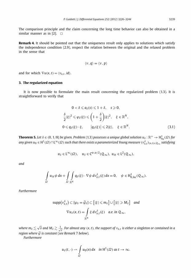
Theorem 5. Let δ ∈ (0,1/8] be given. Problem (1.3) possesses a unique global solution uδ : R+ → H1

u0(Ω) for

any given u0 ∈ H1(Ω)∩L∞(Ω) such that there exists a parameterized Young measure (νδx,t)(x,t)∈Q ∞ satisfying

uδ ∈ L∞(Ω), uδ ∈ Cα,α/2(Q ∞), uδt ∈ L2(Q ∞),

and

∫Ω

uδtψ dx +∫Ω

∫RN

qδ(ξ) · ∇ψ dνδx,t(ξ)dx = 0, ψ ∈ H1

0,loc(Q ∞).

Furthermore

supp(νδ

x,t

) ⊂ [ϕδ = ϕδ] ⊂ [|ξ | � mδ

] ∪ [|ξ | � Mδ

]and

∇uδ(x, t) =∫

RN

ξ dνδx,t(ξ) a.e. in Q ∞,

where mδ �√

δ and Mδ � 1√δ

. For almost any (x, t), the support of νx,t is either a singleton or contained in a

region where ϕ is constant (see Remark 7 below).Furthermore

uδ(t, ·) ⇀

∫Ω

u0(x)dx in H1(Ω) as t → ∞.


Proof. It is a consequence of (3.1) that Theorem 3 applies to the forward–backward equation (1.3).Thus existence of a weak Young measure valued solution u : [0,∞) → H1

u0(Ω) follows. The compari-

son principle and the assumption that u0 ∈ L∞(Ω) entail that

∥∥u(t, ·)∥∥∞ � ‖u0‖∞, t � 0.

Hölder regularity of u follows from the fact that it is in fact a bounded weak solution of

ut = ∇ · pδ(∇u) for t > 0 in Ω,

that δ|ξ |2 � pδ(ξ) · ξ � C |ξ |2, ξ ∈ RN , and from [40,41]. Notice that pδ = ∇ϕδ for the convexification

ϕδ of ϕδ . It therefore satisfies the claimed classical regularity for some positive α. Next using theresult about the support of the Young measure contained in Theorem 3, computing the locationswhere convexity inversion occurs for ϕδ , and estimating the locations where ϕδ and ϕδ touch, it isstraightforward to verify the claim about the support of νx,t . Next observe that

[ξ · qδ(ξ) = 0

] ∩ [ϕδ = ϕδ] = {0}

which, by Theorem 3, implies that ∇u∞ ≡ 0 for any potential equilibrium of the evolution. As the av-erage is a conserved quantity of the evolution, a solution originating in u0 must eventually converge toits average, as stated. The Young measure representation of the gradients follows from Theorem 3. �Remark 6. It is easy to see that the convexification ϕδ of ϕδ coincide in a neighborhood of ξ = 0 andof |ξ | = ∞. In the central region, which grows as δ → 0, one has that

ϕ(ξ) = αδ

ξ

|ξ | , ξ ∈ [mδ � |ξ | � Mδ

]for some 0 < αδ → 0 (δ → 0) by rotational symmetry. This helps understand the Γ -convergenceresult of [36] to solutions of the Total Variation flow. Roughly speaking, rescaling is needed in orderto prevent αδ from vanishing in the limit but also erases all information concerning the time scalefor which the onset of oscillations is observed.

Remark 7. Almost everywhere in Q ∞ one has either that suppνx,t is a singleton, in which case

νx,t = δξ for ξ = ξ(x, t) ∈ [ϕ = ϕ],

or is contained in a region where pδ is constant (see the proof of Theorem 3). Due to the rotationalsymmetry of ϕ such regions are radial segments of the form

{r

ξ0

|ξ0|∣∣∣ r ∈ [mδ, Mδ]

}for a ξ0 ∈ R

N ,

which, combined with the requirement that suppν ⊂ [ϕ = ϕ], yields

νx,t = γ δλδx,t

+ (1 − γ )δΛδx,t

,

where λδx,t = mδ

ξ0|ξ0| and Λδx,t = Mδ

ξ0|ξ0| for some ξ0 = ξ0(x, t) ∈ RN , and where γ = γ (x, t) ∈ [0,1].


Fig. 5. Long time behavior of a solution to (1.3).

Remark 8. An interesting consequence of Theorem 5 is that any solution uδ of (1.3) has an essentiallybounded gradient in the backward region where oscillations may occur since

∣∣∇uδ(x, t)∣∣ = ∣∣⟨νδ

x,t, id⟩∣∣ � max

ξ∈supp(νx,t )|ξ | � Mδ < ∞,

because ν is a family of probability measures and Mδ is a bound for the set [ϕ �= ϕ].

Remark 9. It is interesting to observe that solutions of (1.3) are still continuous, while the samecannot be said for all solutions of the limiting PME.

Remark 10. The concept of weak Young measure valued solution for (1.3) is rather natural in hind-sight. It is in fact able to capture the oscillatory behavior of the gradient caused by the attempt ofsolutions to flee the backward regime either developing smaller or larger gradients (see Remark 7)in an alternating fashion. While this might be the generic behavior of global solutions of PME totranscritical initial data, interestingly there do exist global classical solutions which are initially tran-scritical. They clearly need to have a very special structure, but there are whole families of them asshown in [42].

Remark 11. The long time behavior of solutions, that is, the eventual convergence to a trivial steady-state for (1.3) as well as for (PME) has long been observed numerically. It is comforting to have atheoretical confirmation that this is not an artifact due to numerical diffusion but rather a feature ofthe equation. See Figs. 5–6.

Remark 12. When the regularization parameter gets larger than 1/8, the equation loses its forward–backward and degenerate character and possesses global classical solutions.


Fig. 6. Long time behavior of the gradient of a solution to (1.3).

Remark 13. For transcritical initial data there are effectively two times scales of evolution. In theforward and fast regime, the solution quickly tends to become constant, whereas, in the backwardand slow regime, oscillations appear which survive for a long time because they cannot be read-ily damped by the equation as the solution carries very little left-over energy. The oscillations arecaused by the solution attempting to flee the unstable regime by developing gradients of preferredsmall and large size. As δ tends to zero, the preferred slope sizes approach the values 0 and ∞,respectively. This is precisely the phenomenon of staircasing observed in numerical simulations ofPME.

Remark 14. These theoretical results show that a typical solution to (1.3) never develops jumps, thusdoes not suffer from staircasing. Numerical experiments clearly indicate that the latter is replaced,as soon as δ > 0 by a milder form of infinitesimal behavior, which could appropriately be calledmicro-structured ramping. Solutions with transcritical initial data will develop regions of instabilityin between fast forming macro-plateaus where oscillations of higher and higher frequency (in thesense of approximating sequences) are generated in an attempt to escape the unstable regime. It isalso apparent that the oscillations are between two preferred states with almost vanishing and evergrowing slope (in terms of δ), respectively. This behavior is illustrated in Fig. 7 where the horizontallines represent approximations to the locations where the energy function switches convexity and aresimultaneously upper or lower bounds for the preferred gradient values. This behavior is capturedtheoretically by the concept of Young measure solution and by the location of the support of thegradient Young measure associated to the solution.

Acknowledgments

The author would like to thank Maria Colombo, Marina Ghisi, and Massimo Gobbino for interestingdiscussions and for drawing his attention to the validity of inequality (2.6).


Fig. 7. The ramping phenomenon which replaces staircasing of PME and to which it converges in the vanishing limit of theregularization.

This research was partially supported by the National Science Foundation under award numberDMS-0712875.

References

[1] D. Kinderlehrer, P. Pedregal, Weak convergence of integrands and the Young measure representation, SIAM J. Math.Anal. 23 (1) (1992) 1–19.

[2] S. Demoulini, Young measure solutions for a nonlinear parabolic equation of forward–backward type, SIAM J. Math. Anal. 27(1996) 376–403.

[3] P. Perona, J. Malik, Scale-space and edge detection using anisotropic diffusion, IEEE Trans. Pattern Anal. Mach. Intell. 12(1990) 161–192.

[4] S. Taheri, Q. Tang, K. Zhang, Young measure solutions and instability of the one-dimensional Perona–Malik equation,J. Math. Anal. Appl. 308 (2005) 467–490.

[5] K. Zhang, Existence of infinitely many solutions for the one-dimensional Perona–Malik model, Calc. Var. 26 (2) (2006)171–199.

[6] B. Kawohl, N. Kutev, Maximum and comparison principle for one-dimensional anisotropic diffusion, Math. Ann. 311 (1)(1998) 107–123.

[7] F. Smarrazzo, A. Tesei, On a class of equations with variable parabolicity direction, Discrete Contin. Dyn. Syst. 22 (3) (2008)729–758.

[8] F. Smarrazzo, A. Tesei, Long-time behavior of solutions to a class of forward–backward parabolic equations, SIAM J. Math.Anal. 42 (3) (2010) 1046–1093.

[9] F. Smarrazzo, A. Tesei, Long-time behaviour of two-phase solutions to a class of forward–backward parabolic equations,Interfaces Free Bound. 12 (3) (2010) 369–408.

[10] G. Barenblatt, M. Bertsch, R.D. Passo, M. Ughi, A degenerate pseudoparabolic regularization of a forward–backward heatequation arising in the theory of heat and mass exchange in stably stratified turbulent shear flow, SIAM J. Math. Anal. 24(1993) 1414–1439.

[11] P. Plotnikov, Equations with alternating direction of parabolicity and the hysteresis effect, Russian Acad. Sci. Dokl. Math. 47(1993) 604–608.

[12] P. Plotnikov, Passing to the limit with respect to viscosity in an equation with variable parabolicity direction, Differ. Equ. 30(1994) 614–622.

[13] P. Plotnikov, Forward–backward parabolic equations and hysteresis, J. Math. Sci. 93 (1999) 747–766.


[14] F. Catté, P.-L. Lions, J.-M. Morel, T. Coll, Image selective smoothing and edge-detection by non-linear diffusion, SIAM J.Numer. Anal. 29 (1) (1992) 182–193.

[15] P. Guidotti, J. Lambers, Two new nonlinear nonlocal diffusions for noise reduction, J. Math. Imaging Vision 33 (1) (2009)25–37.

[16] P. Guidotti, A new well-posed nonlinear nonlocal diffusion, Nonlinear Anal. 72 (2010) 4625–4637.[17] P. Guidotti, A new nonlocal nonlinear diffusion of image processing, J. Differential Equations 246 (12) (2009) 4731–4742.[18] M. Nitzberg, T. Shiota, Nonlinear image filtering with edge and corner enhancement, IEEE Trans. Pattern Anal. Mach. In-

tell. 14 (1992) 826–833.[19] G.-H. Cottet, L. Germain, Image processing through reaction combined with nonlinear diffusion, Math. Comp. 61 (204)

(1993) 659–673.[20] J. Weickert, Anisotropic diffusion in image processing, PhD thesis, Universität Kaiserslautern, Kaiserslautern, 1996.[21] G.-H. Cottet, M.E. Ayyadi, A Volterra type model for image processing, IEEE Trans. Image Process. 7 (1998) 292–303.[22] A. Belahmidi, Equations aux dérivées partielles appliquées à la restoration et à l’agrandissement des images, PhD thesis,

Université Paris-Dauphine, Paris, 2003.[23] A. Belahmidi, A. Chambolle, Time-delay regularization of anisotropic diffusion and image processing, M2AN Math. Model.

Numer. Anal. 39 (2) (2005) 231–251.[24] H. Amann, Time-delayed Perona–Malik problems, Acta Math. Univ. Comenian. LXXVI (2007) 15–38.[25] A. Bellettini, G. Fusco, The Γ -limit and the related gradient flow for singular perturbation functionals of Perona–Malik

type, Trans. Amer. Math. Soc. 360 (9) (2008) 4929–4987.[26] S. Kichenassamy, The Perona–Malik paradox, SIAM J. Appl. Math. 57 (5) (1997) 1328–1342.[27] M. Gobbino, Entire solutions of the one-dimensional Perona–Malik equation, Comm. Partial Differential Equations 32 (4–6)

(2007) 719–743.[28] M. Ghisi, M. Gobbino, Gradient estimates for the Perona–Malik equation, Math. Ann. 3 (2007) 557–590.[29] S. Kichenassamy, The Perona–Malik method as an edge pruning algorithm, J. Math. Imaging Vision 30 (2008) 209–219.[30] M. Ghisi, M. Gobbino, A class of local classical solutions of Perona–Malik equation, Trans. Amer. Math. Soc. 361 (12) (2009)

6429–6446.[31] S. Esedoglu, An analysis of the Perona–Malik scheme, Comm. Pure Appl. Math. 54 (2001) 1442–1487.[32] G. Bellettini, M. Novaga, M. Paolini, C. Tornese, Classification of the equilibria for the semi-discrete Perona–Malik equation,

Calcolo 46 (4) (2009) 221–243.[33] G. Bellettini, M. Novaga, M. Paolini, Convergence for long-times of a semidiscrete Perona–Malik equation in one dimension,

Math. Models Methods Appl. Sci. 21 (2) (2008) 241–265.[34] V. Padròn, Sobolev regularization of a nonlinear ill-posed parabolic problem as a model for aggregating populations, Comm.

Partial Differential Equations 23 (1998) 457–486.[35] D. Horstmann, K. Painter, H. Othmer, Aggregation under local reinforcement, from lattice to continuum, European J. Appl.

Math. 15 (2004) 545–576.[36] M. Colombo, M. Gobbino, Passing to the limit in maximal slope curves: from a regularized Perona–Malik equation to the

total variation flow, preprint.[37] M. Chipot, D. Kinderlehrer, Equilibrium configurations of crystals, Arch. Ration. Mech. Anal. 103 (3) (1988) 237–277.[38] L. Evans, Weak Convergence Methods for Nonlinear Partial Differential Equations, CBMS Reg. Conf. Ser. Math., AMS, Provi-

dence, RI, 1990.[39] M. Valadier, A course on young measures, in: Workshop on Measure Theory and Real Analysis, Rend. Istit. Mat. Univ.

Trieste 26 (1994) 349–394.[40] J. Moser, A Harnack inequality for parabolic differential equations, Comm. Pure Appl. Math. XVII (1964) 101–134.[41] J. Moser, Correction to “A Harnack inequality for parabolic differential equations”, Comm. Pure Appl. Math. XX (1967)

231–236.[42] M. Ghisi, M. Gobbino, An example of global classical solution for the Perona–Malik equation, Comm. Partial Differential

Equations 36 (8) (2011) 1318–1352.

a backward–forward regularization of the perona–malik …gpatrick/source/papers/g121.pdf ·...

Documents