A base stock inventory model with possibility of rushing part of order∗

Harry Groenevelt • Nils Rudi

Simon School, University of Rochester, Rochester, NY 14627

groenevelt@simon.rochester.edu • rudi@simon.rochester.edu

December 2003

Abstract

This article studies a situation where a firm outsources production to a distant manufacturer.

The firm has two possible freight modes; a slow mode and a fast but more expensive mode. We

formulate a dynamic model and use it to analyze how the firm can combine these two freight modes

to enjoy the lower cost of the slow mode while using the fast mode as a hedge against cases in which

the demand during the production lead time is high. The structure of the optimal solution of this

dual freight mode strategy is in the form of a nested order-up-to policy. Several properties of the

solution are characterized and these are compared to the case of deterministic demand and the two

pure mode strategies. The analytical findings are extensively illustrated by numerical investigations

throughout the paper.

1 Introduction

To succeed in today’s markets, firms are facing increasing pressure on price as well as on their re-

sponsiveness to volatile market conditions. Price pressure has led to increased sourcing from low-cost

countries, primarily from the Far East. A notable consequence has been increased lead times, which,

in turn, lead to reduced responsiveness to the market. To counter this, several Supply Chain ini-

tiatives have evolved, such as the use of faster freight, Quick Response, variety postponement, and

assembly-to-order based on component commonality.∗We would like to thank Sigrid Lise Nonas, Asmund Olstad, Michal Tzur and Yu-Sheng Zheng for helpful discussions.

Helpful feedback was provided by seminar participants at INSEAD, New York University, University of Oslo and University

of Rochester, as well as from participants at the 2001 Multi-echelon conference at Berkeley on an older version of the

paper.

1

Consider a firm that outsources production to a distant low-cost country. The first part of the lead

time will consist of production (from placing an order to the order being ready for shipping), and the

second part of the lead time will consist of shipping (from the order being ready for shipping until

it is available to the firm). The firm can choose from two alternative modes of shipping: a low-cost

slow mode (e.g., sea freight) or a fast but more expensive mode (e.g., air freight). An issue of interest

is then how to characterize the advantages and disadvantages of the two freight modes, as well as

how to prescribe the choice between them. A third alternative is to combine the two freight modes.

One can then postpone the decision of the mix of the freight modes until the demand during the first

(production) part of the lead time is known. So then, if the demand during the production lead time

is rather low, the firm is likely to possess sufficient inventory to cover the demand during the lead time

of the slow freight mode and use of the expensive freight mode can be avoided. On the other hand, if

the demand during the production lead time is rather high, some (or all) of the produced quantity can

be rushed using the fast freight mode to cover shortages that would otherwise be likely to occur. The

additional demand information can be used to improve the performance over each of the two static pure

freight mode strategies. Hence, using the dual freight strategy provides a hedge for cases in which the

demand during the production lead time is rather high. Combining the two freight modes makes the

firm able to enjoy low freight cost on a large portion of the total demand while still being responsive

through the use of the fast freight mode when needed. Several questions are of interest to firms facing

such decisions: How does the opportunity of rushing part of an order affect the decision of optimal

inventory policy? To what degree should the firm rely on the fast freight mode? What is the impact in

terms of cost reduction of using the dual freight mode strategy? This paper addresses, among others,

these issues.

The scenario studied in this paper is closely related to existing work on the use of express orders and

expediting. The classical serial multistage model of Clark and Scarf (1960) can already be interpreted

as giving the decision-maker some form of control over the total lead time: by leaving units at a stage

for one or more periods, the lead time (i.e. the time it takes the unit to reach the most downstream

stage and be available to satisfy final customer demand) can be extended, while sending the unit on

to the next stage minimizes the total lead time. Of course in Clark and Scarf’s model this means that

the longer a unit stays in the upper stages (the longer the lead time) the more expenses are incurred.

This shortcoming is addressed by Lawson and Porteus (2000), who extend the Clark and Scarf model

by allowing expediting at each stage (i.e., a unit can either be sent to the next stage in the regular

lead time of one period, or it can be expedited at some additional cost and reach the next stage in

2

zero periods). They show that a “top-down base stock policy” is optimal for their model. However,

as Lawson and Porteus state in their conclusion, their model cannot accurately represent the situation

we examine, where the two supply modes differ in their lead time by an amount different from a single

review period. We refer to Lawson and Porteus for a discussion of additional multi-echelon papers with

expediting.

There are also a number of single echelon models with emergency replenishment or multiple supply

sources. A key difference between these papers and ours is that while we consider a single (production)

quantity, some of which can be rushed, models in the literature assume two or more independent supply

alternatives with different lead times and costs. The initial work on the use of express orders, such as

Barankin (1961) and Daniel (1962), are periodic review models where the lead time of the regular order

is one period while the express order has zero lead time. Fukuda (1964) generalizes this to a model with

two supply sources where the lead times differ by one period, and a model with three supply sources

with lead times of three consecutive integers and orders are placed every other period. Whittemore

and Saunders (1977) consider the more general case where the two lead times can take any value

that is a multiple of the review period length. Their resulting optimal policy is extremely complex in

nature. Related models are studied in Gross and Soriano (1972), where in each review period the firm

chooses only one of the supply modes, and Chiang and Gutierrez (1996), who extend this to allow the

express replenishment to have a non-zero lead time that is shorter than the review period, but the cost

expressions are approximations. Moinzadeh and Nahmias (1988) formulate a continuous review model

where regular orders are placed according to a standard reorder point model and express orders can

be placed during the lead time of the regular order. They develop a heuristic approach where neither

the reorder point nor the order quantity for express orders depends on the time remaining of the lead

time of the regular order. Tagaras and Vlachos (2001) have a periodic review model that differs from

Moinzadeh and Nahmias in that the orders are placed at specific review times while the quantities

are variable. Moinzadeh and Schmidt (1991) analyze a continuous review (S-1, S) model with the

possibility of express orders assuming Poisson demand. A common characteristic of all these models

with two or more independent supply alternatives is that the problems are inherently complex to solve,

which leads to complex optimal policies or to the necessity of simplification and approximations in

order to achieve solutions, or both. In our differing model setup, we are able to get exact solutions as

well as several interesting structural properties. Haggins and Olsen (2003) show that (s,S) policies are

optimal in a discrete time, discrete demand model where “expediting” can be used to satisfy unmet

demand in a period.

3

A class of models that are different in setting but similar in spirit are the ones that combine cheap

specific resources, that only can satisfy the corresponding demand classes, with more expensive flexible

resources, that can satisfy any demand class. Examples include Fine and Freund (1990), Van Mieghem

(1997) and Rudi and Zheng (1997). Van Mieghem and Rudi (2001) formulate and analyze a rather

general framework for this type of problems in multi-period settings. Seifert, Thonemann and Hausman

(2001) consider the combination between forward buying and trading in a more flexible spot market

at a higher price in expectation.

When modeling periodic review inventory systems, starting with Arrow, Harris and Marschak (1951)

and Bellman, Glicksberg and Gross (1955), the most frequently used approach to account for inventory

dependent costs is as a function of end-of-period inventory. Specifically, each positive unit of inventory

at the end of a period incurs a unit holding cost and each negative unit of inventory (i.e., demands

not met directly from inventory) incurs a unit penalty cost. Hadley and Whitin (1963) consider an

approximation of the average inventory level during the period by assuming no demand uncertainty

and Moses and Seshadri (1999) use the average of starting and ending period inventory levels as an

approximation to the average inventory during the period. In this paper, we account for inventory

dependent costs in continuous time. Hadley and Whitin (1963) formulate several similar periodic

review models with Poisson and Normal demand. However, they do not obtain analytical solutions.

In a recent paper, Rao (2002), independently of our paper, studies a model similar to our pure freight

mode scenario. His focus is, however, on studying worst-case performance of heuristic ways of setting

the length of the review period with extensions to joint replenishment and multi echelon scenarios.

The remainder of the paper is organized as follows. Section 2 describes the model scenario, its cost

accounting and appropriate demand processes. For demand processes of Normal increments, Section 3

analyzes the use of a pure (single) freight mode and Section 4 analyzes the dual freight mode problem.

In Section 5 we treat the case of Compound Poisson demands and Section 6 gives concluding remarks.

2 Model

We consider a periodic review model where the firm places a production order every T time units.

Unmet demands are assumed to be backlogged. At the completion of production, which has lead time

L1, the firm decides how much to ship using the slow freight mode with lead time L2 and how much

to ship using the fast freight mode with lead time l2. The total lead time of the production and slow

freight is denoted by L = L1 +L2. The only assumption made on the relationship between the decision

4

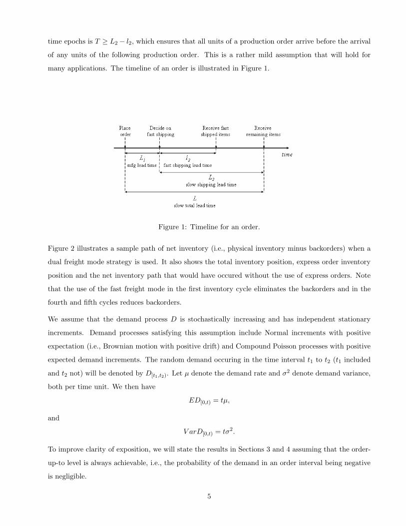
time epochs is T ≥ L2 − l2, which ensures that all units of a production order arrive before the arrival

of any units of the following production order. This is a rather mild assumption that will hold for

many applications. The timeline of an order is illustrated in Figure 1.

Figure 1: Timeline for an order.

Figure 2 illustrates a sample path of net inventory (i.e., physical inventory minus backorders) when a

dual freight mode strategy is used. It also shows the total inventory position, express order inventory

position and the net inventory path that would have occured without the use of express orders. Note

that the use of the fast freight mode in the first inventory cycle eliminates the backorders and in the

fourth and fifth cycles reduces backorders.

We assume that the demand process D is stochastically increasing and has independent stationary

increments. Demand processes satisfying this assumption include Normal increments with positive

expectation (i.e., Brownian motion with positive drift) and Compound Poisson processes with positive

expected demand increments. The random demand occuring in the time interval t1 to t2 (t1 included

and t2 not) will be denoted by D[t1,t2). Let µ denote the demand rate and σ2 denote demand variance,

both per time unit. We then have

ED[0,t) = tµ,

and

V arD[0,t) = tσ2.

To improve clarity of exposition, we will state the results in Sections 3 and 4 assuming that the order-

up-to level is always achievable, i.e., the probability of the demand in an order interval being negative

is negligible.

5

The firm incurs unit holding cost h and unit shortage cost p, both per time unit. It is assumed that

the firm pays on delivery, which results in holding cost being charged on physical inventory. The use of

the fast freight mode incurs an additional unit freight cost cf . The firm seeks to minimize the long-run

expected controllable costs, which is equivalent to minimizing the expected controllable costs per order

cycle.

Figure 2: Example of inventory path.

We use the following base case example throughout the paper. The time between placing production

orders is T = 1. Lead times are: L1 = 0.3 for production, L2 = 0.6 for slow freight, and l2 = 0.3

for fast freight. Per time unit inventory related costs are holding cost per unit of inventory h = 1

and penalty cost per unit of backlog p = 10, and the additional unit freight cost of using fast freight

is cf = 0.5. Finally, the expected demand per time unit is µ = 16 with standard deviation per time

unit σ = 4. While Figure 2 uses the Poisson demand process to illustrate a possible inventory path of

this example, for the numerical illustrations in the remainder of the paper we will employ a demand

process where the increments are Normally distributed. The detailed treatment of the model is done

for demand processes of Normal increments in Sections 3 and 4; analytical results for the Compound

Poisson process are analogous and are summarized in Section 5.

3 Pure freight modes

We will here analyze the case of using only one of the two alternative freight modes. Let sub-

script/superscript s denote the slower freight mode and subscript/superscript f denote the fast freight

mode.

Define x+ = min(0, x). Consider the slower freight mode. At time t′ (the beginning of an order cycle),

6

the firm orders up to quantity S. This order will then affect the inventory level (or, more precisely,

the net inventory level) during the time interval [t′ + L, t′ + L + T ). The inventory level at any time

t ∈ [t′ + L, t′ + L + T ) is then given by S − D[t′,t), where a negative inventory represents backlogs. At

time t, the firm will then incur holding/stockout cost at rate G(S,D[t′,t)

), where

G (y, d) = h (y − d)+ + p (d − y)+ .

The cost affected by a specific order as a function of the order up to level S for the slow freight mode

can then be written as

Cs (S) = E

∫ L+T

LG(S,D[0,t)

)dt

=∫ L+T

LEG

(S,D[0,t)

)dt. (1)

Correspondingly, the cost affected by a specific order as a function of the order-up-to level S for the

fast freight mode can be written as

Cf (S) = cfµT +∫ L1+l+T

L1+lEG

(S,D[0,t)

)dt.

Without loss of generality, we consider the slower freight mode. The following proposition provides the

optimality condition for the ordering policy:

PROPOSITION 1 The expected cycle cost given in (1) is optimized by Ss, which is the value of S such

that1T

∫ L+T

LPr(D[0,t) < S

)dt =

p

p + h. (2)

PROOF: All proofs are given in the appendix. 2

Hadley and Whitin (1963) in their Appendix 4 give a (rather lengthy) expression for the left-hand side

of (2) that involves only evaluations of the standard normal cdf and pdf at various points, (as well as

other elementary operations) that can readily be implemented in a computer program.

The optimality condition (2) allows some interesting insights. Under an optimal solution, the inventory

is, in expectation, positive p/(p + h) of the time and the inventory is, in expectation, negative the

remainder h/(p+h) of the time. This provides an easy to apply rule of thumb for setting the inventory

policy. Note that the optimality condition resembles the optimality condition of the classic newsvendor

problem. The difference is that, while the newsvendor solution prescribes a probability of satisfying all

demands, this solution specifies the expected proportion of time that arriving demands can be satisfied

directly from inventory, also refered to as the fill rate. 1

1We refer to Groenevelt and Rudi (2002) for discussion of settings where the probability of demand between two

consecutive ordering instants being negative is not negligible.

7

The next proposition provides additional properties and insights into the analysis of Cs (S).

PROPOSITION 2 Let Cs (S) represent the deterministic case of Cs (S) (i.e., no demand uncertainty)

with optimizer Ss. We have the following results:

(a) The optimizer of Cs (S) is given by Ss = µL+ pp+hµT with corresponding cost Cs

(Ss)

= 12

hph+pµT 2.

(b) limS→−∞[Cs (S) − Cs (S)

]= 0, and limS→∞

[Cs (S) − Cs (S)

]= 0.

(c) limS→−∞ C ′s (S) = limS→−∞ C ′

s (S) = −pT , and limS→∞ Cs (S) = limS→∞ Cs (S) = hT .

(d) Define the right-hand side linear unit Normal loss function as R (u) =∫∞u (x − u) φ (x) dx. Then,

for demand processes with Normal increments,

Cs (S) = Cs (S) + (h + p)∫ L+T

L

√tσR

( |S − µt|√tσ

)dt. (3)

Proposition 2d implies the following Corollary.

COROLLARY 1 Cs (S) is increasing in the standard deviation σ for any S. It follows as special cases

that Cs (Ss) is increasing in σ and that Cs (Ss) ≥ Cs

(Ss).

Proposition 2 and Corollary 1 offer several insights into the behavior of Cs (S). When the de-

mand process is deterministic, the solution resembles the EOQ model with backlog adjusted for pre-

determined order interval and non-zero lead time. As S becomes sufficiently small, Cs (S) approaches

the deterministic cost function Cs (S) with slope −pT , and, similarly, as S becomes sufficiently large,

Cs (S) approaches the deterministic cost function Cs (S) with slope hT .

We next turn to the relationship between the inventory holding cost h and the penalty cost p. Clearly,

from (2), Ss is increasing in p/(p + h). Letting p + h be fixed at its base value 11, Figure 3 illustrates

the effect of varying p from 1 to 10 in steps of 1. Recall that in the standard newsvendor model with

a symmetric demand distribution (e.g., the normal distribution), for a fixed sum of unit overage and

unit underage costs the maximum expected opportunity cost (i.e., total cost of demand uncertainty

consisting of overage and underage costs) is achieved when setting these two equal (with the corre-

sponding optimal order quantity being equal to the expected demand). Our model closely resembles

the newsvendor model with one fundamental difference: the costs are integrated over a time interval

where the standard deviation of cumulative demand since the last order was placed is increasing in the

time since its placement. This means that the demand variability (in terms of cumulative demand since

the last order was placed) is low early in the cycle when the inventory is positive (just after receiving

an order), relative to later in the cycle when the inventory level is more likely to be negative (just

8

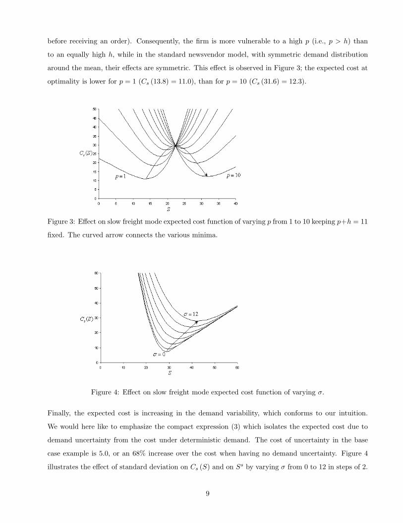
before receiving an order). Consequently, the firm is more vulnerable to a high p (i.e., p > h) than

to an equally high h, while in the standard newsvendor model, with symmetric demand distribution

around the mean, their effects are symmetric. This effect is observed in Figure 3; the expected cost at

optimality is lower for p = 1 (Cs (13.8) = 11.0), than for p = 10 (Cs (31.6) = 12.3).

Figure 3: Effect on slow freight mode expected cost function of varying p from 1 to 10 keeping p+h = 11

fixed. The curved arrow connects the various minima.

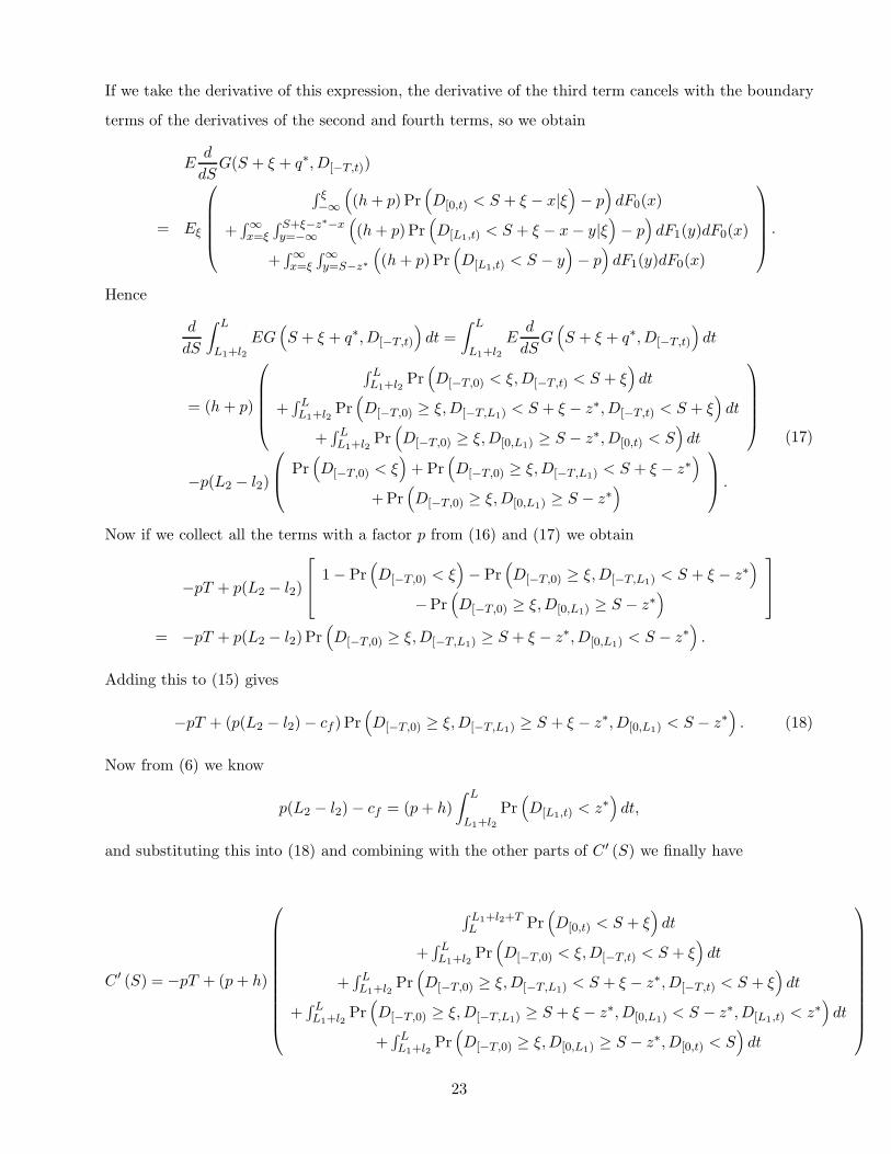
Figure 4: Effect on slow freight mode expected cost function of varying σ.

Finally, the expected cost is increasing in the demand variability, which conforms to our intuition.

We would here like to emphasize the compact expression (3) which isolates the expected cost due to

demand uncertainty from the cost under deterministic demand. The cost of uncertainty in the base

case example is 5.0, or an 68% increase over the cost when having no demand uncertainty. Figure 4

illustrates the effect of standard deviation on Cs (S) and on Ss by varying σ from 0 to 12 in steps of 2.

9

Following up the discussion of the relationship between p and h, when these take their base example

values, Ss is adjusted up from Ss. Figure 4 indicates that this adjustment is amplified as σ increases.

The next lemma compare the two freight modes:

LEMMA 1 The two pure freight modes are related as follows:

(a) Cs

(Ss)

= Cf

(Sf)− cfµT .

(b) limS→−∞ [Cf (S) − Cs (S)] = cfµT − pµ (L2 − l2) T , and limS→∞ [Cf (S) − Cs (S)] = cfµT +

hµ (L2 − l2)T .

(c) Sf < Ss.

(d) Assume that the demand process has Normal increments. Cs (Ss) ≤ Cf

(Sf)

iff

(h + p)∫ L+T

L

√tσR

( |Ss − µt|√tσ

)dt ≤ cfµT + (h + p)

∫ L1+l2+T

L1+l2

√tσR

∣∣∣Sf − µt∣∣∣

√tσ

dt.

As one might expect, the shorter lead time of the fast freight mode does not lead to any benefits

over the slow freight mode, only of extra freight costs. Further, we are able to characterize insightful

relationships in terms of the behavior of the cost functions, as well as the optimal policies, between the

two freight modes.

We refer to Groenevelt and Rudi (2002) for a more in-depth treatment of the pure freight modes.

4 Dual freight mode

We now move on to consider the case of dual freight modes, i.e., the combination of the slow but

cheaper and the fast but more expensive modes. We assume that the retailer places production orders

at times −T , 0, T , etc. – each time to bring the inventory position up to the level S. Hence the

production order placed at time 0 will be for D[−T,0) units of product. At time L1 the firm decides how

to allocate the produced quantity between the two freight modes, knowing both the production order

quantity D[−T,0) and the inventory position excluding the most recent production order S − D[−T,L1).

This is the relevant inventory position for the fast freight order, since the production order placed at

time 0 will not be available to the retailer before time L unless the retailer decides to use the fast

freight mode. Let q be the quantity shipped using the fast freight mode. The (random) cost incurred

during this order cycle is then

cfq +∫ L

L1+l2G(q + S,D[−T,t)

)dt +

∫ L1+l2+T

LG(S,D[0,t)

)dt. (4)

10

Next, we consider the optimal use of the fast freight mode.

PROPOSITION 3 For an arbitrary S, the following use of the fast freight mode is optimal at time L1:

If cf ≥ (L2 − l2)p then q∗ = 0, otherwise

q∗ = min(

D[−T,0),(z∗ − S + D[−T,L1)

)+)

, (5)

where z∗ is the solution to

1L2 − l2

∫ L

L1+l2Pr(D[L1,t) < z

)dt =

p − cf

L2−l2

p + h, (6)

with respect to z.

Notice that the optimal fast freight mode order-up-to quantity z∗ does not depend on the production

order-up-to quantity S. This implies that the problem of finding an optimal combination of fast

shipping policy and production policy can be reduced to the sequential process of first finding z∗ and

then deciding on S∗ (given z∗). Furthermore, the unconstrained optimality condition (6) has a nice

intuitive interpretation. The RHS of (6) is the familiar ratio p/(p + h) adjusted down due to the

additional unit cost of the fast freight mode cf . In the case of the pure freight mode, the total shipping

cost is independent of the inventory policy followed (assuming all demand is satisfied), so the per unit

shipping cost does not play a role in determining the optimal policy.

The objective function to consider when deciding S can then be expressed as

C(S) = cfEq∗ +∫ L

L1+l2EG

(S + q∗,D[−T,t)

)dt +

∫ L1+l2+T

LEG

(S,D[0,t)

)dt. (7)

We are now ready to characterize the optimal S.

PROPOSITION 4 The expected cycle cost given in (7) is optimized by S∗, which is the unique value of

S such that

1T

∫ L1+l2+TL Pr

(D[0,t) < S

)dt

+∫ LL1+l2

(Pr(D[−T,t) < S,D[L1,t) ≥ z∗

)+ Pr

(D[0,t) < S,D[L1,t) < z∗

))dt

=

p

p + h. (8)

An intuitive explanation for (8) is the following. Consider the marginal unit of product included in

S. This unit will decrease the penalty cost rate incurred at time t during the cycle by p, unless the

inventory at time t is already positive, in which case the marginal unit will increase the holding cost

rate incurred at time t by h. Hence, if we denote the physical inventory at time t by I(t), we can

write the impact of the marginal unit at time t as −p + (p + h) Pr (I(t) > 0). It is not hard to see that

I(t) > 0 ⇔ D[0,t) < S when L ≤ t < L1 + l2 + T . This follows since at time L the entire production

11

order placed at time 0 will have arrived at the retailer, regardless of the fast shipping decision made

at time L1.

The situation is more complex when L1 + l2 ≤ t < L. Some reflection shows that in this case we have

I (t) > 0 ⇔ D[L1+l2,t) < S − D[−T,L1+l2) + q∗, since the RHS of this last inequality is the amount of

inventory available at time L1 + l2 (after the delivery of q∗ fast shipped units) and no further delivery

takes place until time L > t. Using (5) we obtain

I (t) > 0 ⇔ 0 < S − D[−T,t) + q∗

⇔ 0 < min(S − D[0,t),max

(S − D[−T,t), z

∗ − D[L1,t)

))

⇔(z∗ > D[L1,t) and S > D[0,t)

)or(z∗ ≤ D[L1,t) and S > D[−T,t)

).

Hence, the integrand of the last integral in (8) equals Pr (I (t) > 0) for L1 + l2 ≤ t < L, and (8) says

nothing other than1T

∫ L1+l2+T

L1+l2Pr (I(t) ≥ 0) dt =

p

p + h.

Note that if cf ≥ (L2 − l2) p, then z∗ = −∞ and the optimality condition (8) reduces to the optimality

condition of the pure slow mode (2) and S∗ = Ss.

We then move on to characterize properties of the dual freight mode problem.

PROPOSITION 5 Let C (S, z) represent the deterministic case of C (S) (i.e., no demand uncertainty)

with optimizers(S∗, z∗

)and let C (S) = C (S, z∗). We have the following results:

(a) If cf < min ((L2 − l2) p, (T − (L2 − l2))h), then the optimizers of C (S, z) are given by

S∗ = µL +p

p + hµT −

p − cf

L2−l2

p + hµ (L2 − l2)

and

z∗ = µl2 +p − cf

L2−l2

p + hµ (L2 − l2) ,

otherwise it is optimal to only use the slow mode. The corresponding cost is given by

C(S∗, z∗

)=

12

hp

h + pT 2µ − ((L2 − l2) p − cf )+ ((T − (L2 − l2))h − cf )+

h + pµ.

(b) limS→−∞ C (S) = limS→−∞ C (S) = limS→−∞ Cs (S)−(p (L2 − l2) − cf )+ µT , and limS→∞ C (S) =

limS→∞ C (S) = limS→∞ Cs (S).

(c) limS→−∞ C ′ (S) = limS→−∞ C ′ (S) = −pT , and limS→∞ C ′ (S) = limS→∞ C ′ (S) = hT .

12

(d) min (Cs (S) , Cf (S)) ≥ C (S) ≥ Cs (S) − (p (L2 − l2) − cf )+ µT and C ′f (S) ≥ C ′ (S) ≥ C ′

s (S).

(e) Ss ≥ S∗ ≥ Sf ≥ z∗.

Proposition 5 offers several interesting insights into the behavior of C (S). The case of no demand

uncertainty has an interesting relationship to its equivalent when using only the slow freight mode in

terms of the adjustment of Ss. Also, we have that the deterministic costs at optimality for the dual

freight mode and the slow freight mode are related by

C(S∗, z∗

)= Cs

(Ss)− ((L2 − l2) p − cf )+ ((T − (L2 − l2))h − cf )+

h + pµ,

where the second term on the right-hand side represents the cost savings per cycle achieved by going

from only using the slow freight mode to using a dual freight mode.

Proposition 5b shows that the expected cost approaches the cost of the deterministic problem as S

gets sufficiently small/large. Further, note that for sufficiently small S, the quantity rushed using the

fast mode is equal to the order quantity that cycle (in expectation µT ). This results in a reduction in

penalty cost of p (L2 − l2)µT compared to only using the slow freight mode, at an extra fast freight

expense of cfµT per cycle. For sufficiently large S, the fast freight mode will never be used and the

cost of the dual strategy approaches the cost of only using the slow freight mode.

Much like Cs (S), the slope of C (S) approaches −pT as S becomes sufficiently small and hT as S

becomes sufficiently large.

Figure 5: Expected cost dual freight mode compared to its deterministic case and the two pure freight

modes.

We then turn to illustrating the analytical findings using the base example much like we did for the

pure freight modes. The relationships between C (S), C (S), Cs (S) and Cf (S) are illustrated in Figure

13

5. Comparing the dual freight mode to the slow freight mode, we see that its optimum C (29.1) = 10.7

represents an expected cost saving of 1.6 or 13%. Breaking up this cost difference, we see that it

consists of the difference between the deterministic costs of Cs (28.9) − C (25.3) = 7.3 − 6.5 = 0.8

and the difference between the costs of uncertainty of[Cs (31.6) − Cs (28.9)

]−[C (29.1) − C (25.3)

]=

[12.3 − 7.3]−[10.7 − 6.5] = 0.8. Further, the optimal base stock level of the dual freight mode S∗ = 29.1

is 2.5 less than its slow freight mode counterpart. This is because the option of using the fast freight

for (part of) the production order reduces the need for a high base stock level.

Figure 6: Effect on dual freight mode optimal decisions and corresponding expected cost of varying p

from 1 to 10 keeping p + h = 11 fixed.

The effect of the relationship between p and h on the expected cost at optimality is illustrated in Figure

6, keeping p + h = 11 fixed and varying p from 1 to 10. Also, the optimal decision variables S∗ and

z∗, as well as the expected quantity shipped using the fast freight mode Eq∗, are plotted to illustrate

how they are affected by p/(p + h). Much like the slow freight mode illustrated in Figure 3, C (S∗)

attains its maximum value when p and h are close to equal. As p increases, the consequence of an

underage becomes larger relative to the consequence of an overage, which causes S∗ and z∗ to increase

with p. For p ≤ 5/3, it is, by the condition of Proposition 3, optimal not to use the fast freight mode

at all (i.e., q∗ = 0 and z∗ = −∞). When 5/3 < p ≤ 2.9, z∗ is increasing more rapidly than S∗ with a

corresponding increase in Eq∗. For the majority of p-values (i.e., 2.9 < p), however, Eq∗ is decreasing

even though z∗ is increasing. This is due to the fact that z∗ increases at a slower rate than S∗ for these

values of p, i.e., an increase in S∗ will lead to a corresponding increase in the inventory level at the

time of making the decision of how much to ship by the fast freight mode.

14

Figure 7: Effect on dual freight mode optimal decisions and corresponding expected cost of varying σ.

Similarly, the effect of demand variability is illustrated in Figure 7 by plotting how the optimal decisions

and corresponding expected cost depend on σ. In terms of the cost of uncertainty, comparing Figure 7

with Figure 4 shows that C (S∗) increases more slowly in σ than Cs (Ss). Further, S∗ is increasing at a

faster rate than z∗ in σ. The intuition being this is that S∗ is to cover the uncertainty of a longer time

span (i.e., L + T ) than is z∗ (i.e., L2). There are two main effects of σ on Eq∗: (i) keeping S and z

fixed, a higher σ would increase the expected difference between z and the inventory level at the time

of making the decision of how many units to ship using the fast freight mode, driving Eq∗ up, and (ii)

S∗ increases at a faster rate than z∗ in σ, which means that for a given quantity to be shipped by the

fast freight mode, the demand during the production lead time needs to be larger. From Figure 7 we

see that the first of these effects dominates the second for smaller σ’s and vice versa for larger σ’s.

We then turn to illustrating how the additional cost of using the fast freight affects the attractiveness

of the dual freight mode in Figure 8. Note here that even if cf = 0, the dual freight mode will dominate

the fast freight mode as it is a way to keep the inventory level “closer” to the mean by two effects:

(i) by two inventory replenishments during a cycle, and (ii) by the postponement of the decision of

what proportion of the production order to receive using the fast freight mode. As cf becomes large,

the dual mode policy and its cost approach the case of only using the slow transportation mode, and

for cf ≥ 3 they coincide by the condition of Proposition 3. As expected, to retain the optimal service

level (i.e., positive inventory p/ (p + h) of the time), S∗ is increasing and z∗ is decreasing in cf , with a

resulting decrease of Eq∗ in cf .

In Figure 9 we illustrate the effect of the shipping lead time l2 of the fast freight mode. Intuitively,

we would expect the expected cost of the dual freight mode C (S∗) to be increasing in the fast freight

15

Figure 8: Effect on dual freight mode optimal decisions and corresponding expected cost of varying

the additional shipping cost of the fast freight mode cf .

lead time l2 due to the loss of responsiveness. For small values of the fast freight lead time (l2 < 0.06),

however, C (S∗) is actually decreasing. This can be explained as follows. If the fast freight lead time

is very small, fast shipped units tend to arrive before they are really needed to reduce shortage costs

and the result is higher holding costs. Then C (S∗) is increasing in the lead time of the fast freight for

0.06 ≤ l2 < 11/20. When l2 ≥ 11/20, it is, by the condition of Proposition 3, optimal not to use the

fast freight mode at all (i.e., q∗ = 0 and z∗ = −∞), and as a result C (S∗) = Cs (Ss).

Figure 9: Effect on dual freight mode optimal decisions and corresponding expected cost of varying

the shipping lead time of the fast freight mode l2.

16

Figure 10: Effect on dual freight mode optimal decisions and corresponding expected cost of varying

the production lead time L1, keeping the total lead times L1 + L2 and L1 + l2 fixed.

Finally, in Figure 10 we illustrate the effect of the value of additional information in terms of how

long the decision of what to ship using fast freight can be postponed. Specifically, we keep the total

lead times, i.e., L1 + L2 and L1 + l2, fixed while varying L1 from 0 to 0.6. First note that S∗ is quite

insensitive to changes in L1 and that z∗ is decreasing close to the rate that l2µ is decreasing in L1.

Consequently, Eq∗ is quite insensitive to changes in L1. The realized q∗ will, however, be quite different

as L1 changes as the firm is making the decision of the quantity shipped by fast freight based on better

information. Consequently, the expected cost of the dual mode at optimality C (S∗) decreases from

11.1 when L1 = 0 to 10.2 when L1 = 0.6, or an 8.1% decrease.

5 Compound Poisson demand process

In this section, we show how to calculate the optimal policies for the pure and dual freight mode

problems when the demand process is a compound Poisson process. Because the compound Poisson

process is non-decreasing, the issue of negative demand does not arise in this case. In addition, as we

will see, numerical integration can be avoided completely (in the Normal increments case one needs to

numerically evaluate several double integrals each time C(S) or C ′(S) is calculated), and the formulas

we derive below can be implemented quite efficiently.

Let D[t1,t2) =∑N(t2)

i=N(t1) Xi, where {N(t)} is a Poisson process with rate ν, and X1,X2, ... are independent

and identically distributed discrete positive random variables. We will write rk = Pr{Xi = k}, k =

0, 1, ..., so r0 = 0 by assumption, and of course we have νEXi = µ as the total expected demand per

17

time unit, consistent with the notation in the rest of the paper. Further, define ρ = |{k : rk > 0}|, i.e.,

ρ is the number of positive probabilities in the distribution of Xi.

For t1 ≤ t2 and integer values of s, we define P[t1,t2)(s) =∫ t2t1

Pr{D[0,t) = s

}dt,

H[t1,t2)(s) =∫ t2t1

Pr{D[0,t) < s

}dt, and J[t1,t2)(s) =

∫ t2t1

E[s − D[0,t)

]+dt. These quantities are needed

in calculating the optimal policies and the cost associated with arbitrary policies for both the pure and

dual freight mode problems. Note that P[t1,t2)(s) = H[t1,t2)(s) = J[t1,t2)(s) = 0 for all s < 0, and it is

easy to verify that for s ≥ 0

H[t1,t2)(s) = H[t1,t2)(s − 1) + P[t1,t2)(s − 1),

J[t1,t2)(s) = J[t1,t2)(s − 1) + H[t1,t2)(s).

Hence if P[t1,t2)(k) can be calculated efficiently for all 0 ≤ k ≤ s, so can H[t1,t2)(k) and J[t1,t2)(k).

Define for t ≥ 0 and integer values of s the probabilities wt(s) = Pr{D[0,t) = s

}, and Wt(s) =

Pr{D[0,t) ≤ s

}. These probabilities can be found using the efficient and stable recursion in Adelson

(1966), see also Tijms (1994):

wt(0) = e−νt,

wt(s) =νt

s

s−1∑

k=0

(s − k) rs−kwt(k), s = 1, 2, ... .

PROPOSITION 6 For t1 ≤ t2 and integer values of s we have

P[t1,t2)(s) =1ν

(wt1(s) − wt2(s)) +s−1∑

j=0

rs−jP[t1,t2)(j). (9)

Note that to find P[t1,t2)(k) for k = 0, ..., s requires at most O(s · min(ρ, s)) operations.

Next, we will find the optimal base stock level when only the slow freight mode is used. The total cost

per cycle is given by expression (1):

Cs(S) =∫ T+L

LEG

(S,D[0,t)

)dt

= (h + p)∫ T+L

LE(S − D[0,t)

)+dt + p

∫ T+L

L

(ED[0,t) − S

)dt

= (h + p) J[L,T+L)(S) + pT

(µ

(L +

12T

)− S

).

Define Ss to be the smallest value of S that minimizes Cs(S). To find the minimum cost, it is useful

to look at

∆Cs(S) = Cs(S) − Cs(S − 1)

= (h + p)(J[L,T+L)(S) − J[L,T+L)(S − 1)

)− pT

= (h + p)H[L,T+L)(S) − pT.

18

For S ≤ 0, this reduces to ∆Cs(S) = −pT , and it follows immediately that Ss ≥ 0. Clearly, ∆Cs(S) is

non-decreasing in S , so Cs(S) is convex. Hence, SS is the unique value of S that satisfies

∆Cs(S) < 0 ≤ ∆Cs(S + 1) ⇔ H[L,T+L)(S) <pT

h + p≤ H[L,T+L)(S + 1).

Hence, to find Ss and Cs(Ss) only the values P[L,T+L)(k), k = 0, ..., Ss are needed, and the total amount

of work needed to calculate the optimal policy and evaluate it is O (Ss · min (ρ, Ss)).

Clearly, Proposition 2 and Lemma 1 remain true for the case of compound Poisson demand as long as

we use the difference operator ∆ instead of the derivative where appropriate, and it is possible that

Ss = Sf in lemma 1 part c.

Next, we turn to the dual freight mode problem. Define z∗ to be the smallest minimizer of (see the

proof of Proposition 3):

Γ(z) = cfz +∫ L2

l2EG

(z,D[L1,t)

)dt

= cfz + (p + h)J[l2,L2)(z) − p (L2 − l2)(

z − µ

2(L2 + l2)

)

= (p + h)J[l2,L2)(z) − (p (L2 − l2) − cf ) z + pµ

2

(L2

2 − l22

).

It follows that

∆Γ(z) = Γ(z) − Γ(z − 1) = (p + h)H[l2,L2)(z) − (p (L2 − l2) − cf ) .

For z ≤ 0 we have ∆Γ(z) = − (p (L2 − l2) − cf ), hence when cf ≥ p (L2 − l2), it is optimal never to

use express freight (z∗ = −∞). If cf < p (L2 − l2) then ∆Γ(z) < 0 for z ≤ 0, and so z∗ ≥ 0 and can be

found as the unique value of z that satisfies

∆Γ(z) < 0 ≤ ∆Γ(z + 1) ⇔ H[l2,L2)(z) <p(L2 − l2) − cf

h + p≤ H[l2,L2)(z + 1). (10)

So to find z∗, only the values P[l2,L2)(k) for k = 0, ..., z∗ are needed.

To calculate C(S) we have (see (7)):

C(S) = cfEq∗ +∫ L

L1+l2EG

(S + q∗,D[−T,t)

)dt +

∫ L1+l2+T

LEG

(S,D[0,t)

)dt.

After considerable manipulation, this can be written as

C(S) =

Tµ(cf + p

(L1 + l2 + T

2

))− pTS

+(p (L2 − l2) − cf )∑S−z∗−1

j=0 (WL1(j) − WT+L1(j))

+(p + h)

J[L,L1+l2+T )(S) +∑S−z∗

k=0 wT+L1(k)J[l2 ,L2)(S − k)

(WL1(S − z∗) − WT+L1(S − z∗))J[l2,L2)(z∗)

+∑S−1

k=S−z∗+1 wL1(k)J[l2,L2)(S − k)

. (11)

19

Define S∗ to be the smallest minimizer of C(S). To find S∗, calculate

∆C(S) = C(S) − C(S − 1)

=

(p (L2 − l2) − cf ) (WL1(S − z∗ − 1) − WT+L1(S − z∗ − 1))

+(p + h)

H[L,L1+l2+T )(S)+∑S−z∗−1

k=0 wT+L1(k)H[l2,L2)(S − k)

+∑S−1

k=S−z∗ wL1(k)H[l2,L2)(S − k)

− pT

. (12)

Using (10), one can show that ∆C(S) is non-decreasing, hence C(S) is convex. It follows that optimal

base stock level S∗ is the unique value of S that satisfies ∆C(S) < 0 ≤ ∆C(S + 1). Again, ∆C(S) =

−pT < 0 when S ≤ 0, and so S∗ ≥ 0. It follows that to find S∗ and to calculate C(S∗) we need the values

P[L,L1+l2+T )(k), P[l2 ,L2)(k), and wL1(k) for k = 0, ..., S∗, and wT+L1(k) for k = 0, ..., S∗ − z∗. These can

all be found in O (S∗ · min (ρ, S∗)) time and the work involved is dominated by the convolution in the

inner parentheses of (12). Hence the total complexity is O((S∗)2

), and an analysis of (11) shows that

the cost C (S∗) can be found in O((S∗)2

)as well. Remarkably, assuming Poisson demand (ρ = 1) does

not reduce this complexity. Finally, we note that Proposition 5 remains true (again, use the difference

operator ∆ instead of derivatives in part c, except that it is possible that S∗ = Sf and/or Sf = z∗ in

part e.

6 Conclusion

This paper introduces a model of combining two freight modes of goods shipped from a single vendor.

The model is solved analytically and several interesting properties of the solution are characterized, as

well as its relationship to the case of using a single freight mode. The transparency of the analysis can

facilitate managerial insights into how to manage such systems in a dynamic setting. The analysis is

illustrated by several numerical examples.

Also, we would like to emphasize the usefulness of the solution techniques used, as we believe they can

be applied to a variety of other inventory problems where the inventory-related costs are accounted for

in continuous time.

7 Appendix: proofs

PROOF OF PPROPOSITION 1: By interchangeability of the derivative and expectation, we have that

C ′s (S) =

d

dS

∫ L+T

LEG

(S,D[0,t)

)dt =

∫ L+T

LE

d

dSG(S,D[0,t)

)dt.

20

Taking the derivative yields

C ′s (S) =

∫ L+T

L

[hPr

(D[0,t) < S

)− pPr

(D[0,t) > S

)]dt.

It is easily seen that C ′′s (S) > 0, and hence that Cs(S) is convex and the first order condition guarantees

the global optimum. Equating to zero and rearranging gives the desired result. 2

PROOF OF PROPOSITION 2: The proof is provided in Groenevelt and Rudi (2002).

PROOF OF COROLLARY 1: To prove the desired monotonicity result of Cs (S), it is sufficient to show

that√

tσR

( |S − µt|√tσ

)

is increasing in σ. This follows readily since R (·) is decreasing in its argument. Further, since C ′s (Ss) =

0, we haved

dσCs (Ss) = C ′

s (Ss)∂Ss

∂σ+

∂Cs (Ss)∂σ

=∂Cs (Ss)

∂σ> 0,

proving the monotonicity result of Cs (Ss). Finally, the result Cs (Ss) ≥ Cs

(Ss)

follows from Cs (Ss) ≥

Cs (Ss) ≥ Cs

(Ss).2

PROOF OF Lemma 1: Parts (a), (b) and (d) of this Lemma follow directly from Proposition 2. Part (c)

follows from∫ L+T

LPr(D[0,t) < S

)dt =

∫ L1+l2+T

L1+l2Pr(D[0,t+L2−l2) < S

)dt <

∫ L1+l2+T

L1+l2Pr(D[0,t) < S

)dt,

together with the fact that these integrals are increasing in S.2

PROOF OF PROPOSITION 3: First observe that the last term of (4) does not depend on q, and hence it is

sufficient to consider the first two terms only. Next, when deciding q, the relevant inventory position

is S − D[−T,L1), since the production order placed at time −T will be received in its entirety by time

−T + L (≤ L1 + l2), regardless of the mix of freight modes employed. The unconstrained problem of

ordering up to z units using the fast freight mode can thus be formulated as

minz

[cfz +

∫ L

L1+l2EG

(z,D[L1,t)

)dt

],

which has the first order condition (6) and whose objective function can easily be shown to be convex

in z. If the cost per unit fast shipped cf exceeds the maximum potential benefit derived, (L2 − l2)p,

then obviously no fast shipping takes place, so q∗ = 0. Note that in this case the objective function

is everywhere increasing in z. If cf < (L2 − l2)p one would like to fast ship z∗ − S + D[−T,L1) units.

However, the actual quantity fast shipped must be nonnegative, and furthermore, one cannot fast ship

more than D[−T,0), the size of the production order placed at time 0, hence (5).2

21

PROOF OF PROPOSITION 4: This proof is given allowing for negative demand in any time interval, which

has the case of non-negative demand in any order interval as presented in the paper as a special case. As

in the corresponding discussion of the pure freight mode strategies, let S + ξ be the inventory position

immediately after placing an order at time −T . A minor modification of the proof of Proposition 3

then shows that the optimal fast freight quantity is given by

q∗ =

0 if D[−T,0) < ξ,

0 if D[−T,0) ≥ ξ and D[−T,L1) < S + ξ − z∗,

z∗ + D[−T,L1) − S − ξ if D[−T,0) ≥ ξ and D[−T,L1) ≥ S + ξ − z∗ and D[0,L1) < S − z∗,

D[−T,0) − ξ if D[−T,0) ≥ ξ and D[0,L1) ≥ S − z∗.

(13)

The objective function can now be written as

C (S) = cfEq∗ +∫ L

L1+l2EG

(S + ξ + q∗,D[−T,t)

)dt +

∫ L1+l2+T

LEG

(S + ξ,D[0,t)

)dt, (14)

where all three expectations are w.r.t. ξ as well as the demand process.

From (13) we have

d

dS(cfEq∗) = −cf Pr

(D[−T,0) ≥ ξ,D[−T,L1) ≥ S + ξ − z∗,D[0,L1) < S − z∗

). (15)

The derivative of the last term of (14) is equal to

d

dS

∫ L1+l2+T

LEG

(S + ξ,D[0,t)

)dt =

∫ L1+l2+T

LE

d

dSG(S + ξ,D[0,t)

)dt

=∫ L1+l2+T

L

((h + p)Eξ Pr

(D[0,t) < S + ξ|ξ

)− p

)dt

= −p(l2 + T − L2) + (h + p)∫ L1+l2+T

LPr(D[0,t) < S + ξ

)dt. (16)

To take the derivative of the middle term of (14), note that the four ranges in the definition of (13)

partition the entire probability space. By conditioning on the realizations of D[−T,0) (with CDF F0)

and D[0,L1) (with CDF F1) and considering the four ranges in this definition of q∗, the integrand of the

middle term of (14) can be expressed as

EG(S + ξ + q∗,D[−T,t)

)

= Eξ

∫ ξ−∞ E

(G(S + ξ − x,D[0,t)

)|ξ)

dF0(x)

+∫∞x=ξ

∫ S+ξ−z∗−xy=−∞ E

(G(S + ξ − x − y,D[L1,t)

)|ξ)

dF1(y)dF0(x)

+EG(z∗,D[L1,t)

) ∫∞x=ξ (F1(S − z∗) − F1(S + ξ − z∗ − x)) dF0(x)

+∫∞x=ξ

∫∞y=S−z∗ EG

(S − y,D[L1,t)

)dF1(y)dF0(x)

.

22

If we take the derivative of this expression, the derivative of the third term cancels with the boundary

terms of the derivatives of the second and fourth terms, so we obtain

Ed

dSG(S + ξ + q∗,D[−T,t))

= Eξ

∫ ξ−∞

((h + p) Pr

(D[0,t) < S + ξ − x|ξ

)− p

)dF0(x)

+∫∞x=ξ

∫ S+ξ−z∗−xy=−∞

((h + p) Pr

(D[L1,t) < S + ξ − x − y|ξ

)− p

)dF1(y)dF0(x)

+∫∞x=ξ

∫∞y=S−z∗

((h + p) Pr

(D[L1,t) < S − y

)− p

)dF1(y)dF0(x)

.

Hence

d

dS

∫ L

L1+l2EG

(S + ξ + q∗,D[−T,t)

)dt =

∫ L

L1+l2E

d

dSG(S + ξ + q∗,D[−T,t)

)dt

= (h + p)

∫ LL1+l2

Pr(D[−T,0) < ξ,D[−T,t) < S + ξ

)dt

+∫ LL1+l2

Pr(D[−T,0) ≥ ξ,D[−T,L1) < S + ξ − z∗,D[−T,t) < S + ξ

)dt

+∫ LL1+l2

Pr(D[−T,0) ≥ ξ,D[0,L1) ≥ S − z∗,D[0,t) < S

)dt

−p(L2 − l2)

Pr(D[−T,0) < ξ

)+ Pr

(D[−T,0) ≥ ξ,D[−T,L1) < S + ξ − z∗

)

+Pr(D[−T,0) ≥ ξ,D[0,L1) ≥ S − z∗

)

.

(17)

Now if we collect all the terms with a factor p from (16) and (17) we obtain

−pT + p(L2 − l2)

1 − Pr(D[−T,0) < ξ

)− Pr

(D[−T,0) ≥ ξ,D[−T,L1) < S + ξ − z∗

)

−Pr(D[−T,0) ≥ ξ,D[0,L1) ≥ S − z∗

)

= −pT + p(L2 − l2) Pr(D[−T,0) ≥ ξ,D[−T,L1) ≥ S + ξ − z∗,D[0,L1) < S − z∗

).

Adding this to (15) gives

−pT + (p(L2 − l2) − cf ) Pr(D[−T,0) ≥ ξ,D[−T,L1) ≥ S + ξ − z∗,D[0,L1) < S − z∗

). (18)

Now from (6) we know

p(L2 − l2) − cf = (p + h)∫ L

L1+l2Pr(D[L1,t) < z∗

)dt,

and substituting this into (18) and combining with the other parts of C ′ (S) we finally have

C ′ (S) = −pT + (p + h)

∫ L1+l2+TL Pr

(D[0,t) < S + ξ

)dt

+∫ LL1+l2

Pr(D[−T,0) < ξ,D[−T,t) < S + ξ

)dt

+∫ LL1+l2

Pr(D[−T,0) ≥ ξ,D[−T,L1) < S + ξ − z∗,D[−T,t) < S + ξ

)dt

+∫ LL1+l2

Pr(D[−T,0) ≥ ξ,D[−T,L1) ≥ S + ξ − z∗,D[0,L1) < S − z∗,D[L1,t) < z∗

)dt

+∫ LL1+l2

Pr(D[−T,0) ≥ ξ,D[0,L1) ≥ S − z∗,D[0,t) < S

)dt

23

= −pT + (p + h)

∫ L1+l2+TL Pr

(D[0,t) < S + ξ

)dt

+∫ LL1+l2

Pr(D[−T,0) < ξ,D[−T,t) < S + ξ

)dt

+∫ LL1+l2

Pr(D[−T,0) ≥ ξ,D[−T,t) < S + ξ,D[L1,t) ≥ z∗

)dt

+∫ LL1+l2

Pr(D[−T,0) ≥ ξ,D[0,t) < S + ξ,D[L1,t) < z∗

)dt

.

To prove this last equality requires some tedious but straightforward manipulation of the integrands;

we omit the details. Clearly, C ′ (S) is increasing in S, so S∗ solves minS C (S). Finally, optimality

condition (8) is obtained by assuming ξ ≡ 0 and Pr(D[−T,0) ≥ 0

)= 1.2

PROOF OF PROPOSITION 5: The proof is provided in Groenevelt and Rudi (2002).

PROOF OF PROPOSITION 6: By conditioning on the number of arrivals in the underlying Poisson process

we have

P[0,t)(s) =∫ t

0

∞∑

n=0

Pr(D[0,u) = s|N(u) = n

)Pr (N(u) = n) du

=∫ t

0

∞∑

n=0

Pr

(n∑

k=1

Xk = s

)(νu)n

n!e−νudu

=∞∑

n=0

Pr

(n∑

k=1

Xk = s

)∫ t

0

(νu)n

n!e−νudu.

Let R(z) =∑∞

n=0 rnzn be the generating function of {rn}∞n=0. The generating function of{

1t P[0,t)(n)

}∞n=0

is given by

Pt(z) =1t

∞∑

s=0

P[0,t)(s)zs

=1t

∞∑

s=0

(R(z)

)s∫ t

0

(νu)s

s!e−νudu

=1t

∞∑

s=0

(R(z)

)s(

1 − e−νts∑

k=0

(νt)k

k!

)

=1

νt(1 − R(z)

)

1 − e−νt

∞∑

k=0

(νtR(z)

)k

k!

=1 − e−νt(1−R(z))

νt(1 − R(z)

) .

By the standard inversion formula we have for k = 0, 1, ...,

1tP[0,t)(s) =

1k!

dkPt(z)dzk

∣∣∣∣∣z=0

. (19)

Hence (since R(0) = r0 = 0 by assumption), we find 1t P[0,t)(0) = Pt(0) = 1−e−νt

νt . For k > 0,

using (19) directly does not result in very friendly expressions, so instead we define Wt(z) = 1 −

24

νt(1 − R(z)

)Pt(z) = eνt(R(z)−1). Note that Wt(z) is the generating function of {wt(n)}∞n=0, see e.g.,

Tijms(1994). Using Leibnitz’s rule for the differentiation of a product on 1 − νt(1 − R(z)

)Pt(z) we

have for k = 1, 2, ... that

W(k)t (z) = νt

(R(z) − 1

)P

(k)t (z) +

k−1∑

j=0

k

j

R(k−j)(z)P (j)

t (z)

.

It follows that

wt(k) =1k!

W(k)t (0) = ν

−P[0,t)(k) +

k−1∑

j=0

rk−jP[0,t)(j)

and hence

P[0,t)(k) = −1ν

wt(k) +k−1∑

j=0

rk−jP[0,t)(j),

and (9) follows with P[t1,t2)(k) = P[0,t2)(k) − P[0,t1)(k). 2

References

Adelson, R.M. 1966. Compound Poisson distribution. Operations Research Quarterly, Vol. 17, 73-75.

Arrow, K.J., T. Harris and J. Marschak. 1951. Optimal inventory policy. Econometrica, Vol. 19,

250-272.

Barankin, E.W. 1961. A delivery-lag inventory model with an emergency provision. Naval Research

Logistics Quarterly, Vol. 8, 285-311.

Bellman, R.E., I. Glicksberg and O. Gross. 1955. On the optimal inventory equation. Management

Science, Vol. 2, 83-104.

Chiang, C. and G.J. Gutierrez. 1996. A periodic review inventory system with two supply modes.

European Journal of Operations Research, Vol. 94, 527-547.

Clark, A. and H. Scarf. 1960. Optimal policies for the multi-echelon inventory problem. Management

Science, Vol. 40, 475-490.

Daniel, K.H. 1962. A delivery-lag inventory model with emergency. H.E. Scarf, D.M. Gilford and

M.W. Shelly (eds.), Multistage inventory models and techniques. Stanford University Press, Stanford,

CA.

Fine, C.H. and R.M. Freund. 1990. Optimal investment in product-flexible manufacturing capacity.

Management Science, Vol. 36, 449-466.

Fukuda, Y. 1964. Optimal policies for the inventory problem with negotiable leadtime. Management

Science, Vol. 10, 690-708.

25

Groenevelt, H. and N. Rudi. 2002. A base stock inventory model with possibility of rushing part of

order (unabridged version). Technical report, University of Rochester.

Gross, D. and A. Soriano. 1972. On the economic application of airlift to product distribution and its

impact on inventory levels. Naval Research Logistics Quarterly, Vol. 19, 501-507.

Hadley, G. and T.M. Whitin. 1963. Analysis of inventory systems. Prentice-Hall, Englewood Cliffs,

New Jersey.

Haggind, E.L. and T.L. Olsen. 2003. Supply chain management with guaranteed delivery. Working

paper, University of Washington in St. Louis.

Kleinrock, L. 1975. Queuing systems volume I: theory. John Wiley and Sons, New York.

Lawson, D.G. and E.L. Porteus. 2000. Multistage inventory management with expediting. Operations

Research, Vol. 48, 878-893.

Moinzadeh, K.S. and S. Nahmias. 1988. A continuous review model for an inventory system with two

supply modes. Management Science, Vol. 34, 761-773.

Moinzadeh, K.S. and C.P. Schmidt. 1991. An (S-1, S) inventory system with emergency orders. Op-

erations Research, Vol. 39, 308-321.

Moses, M. and S. Seshadri. 1999. Policy mechanisms for supply chain coordination. IEE Transaction,

Vol. 32, 245-262.

Rao, U. 2002. Properties of the periodic review (R,T ) inventory policy for stationary, stochastic de-

mand. Working paper, University of Cincinnati.

Rudi, N. and Y.S. Zheng. 1997. Multi-item newsboy model with partial variety postponement. Pre-

sentation, INFORMS Dallas, October.

Seifert, R.W., U.W. Thonemann and W.H. Hausman. 2001. Optimal procurement strategies for online

spot markets. Working paper, International Institute for Management Development (IMD).

Tagaras, G. and D. Vlachos. 2001. A periodic review inventory system with emergency replenishments.

Management Science, Vol. 47, 415-429.

Tijms, H.C. 1994. Stochastic models: an algorithmic approach. John Wiley and Sons, Chichester,

England.

Van Mieghem, J.A. 1998. Investment strategies for flexible resources. Management Science, Vol. 44,

1071-1078.

Van Mieghem, J.A. and N. Rudi. 2002. Newsvendor networks: dynamic inventories and capacities

with discretionary pooling. Manufacturing & Service Operations Management, Vol. 4, 313-335.

Whittemore, A.S. and S. Saunders. 1977. Optimal inventory under stochastic demand with two supply

options. SIAM Journal of Applied Mathematics, Vol 32, 293-305.

26