a bayesian mark interaction model for analysis of tumor

The Annals of Applied Statistics2019, Vol. 13, No. 3, 1708–1732https://doi.org/10.1214/19-AOAS1254© Institute of Mathematical Statistics, 2019

A BAYESIAN MARK INTERACTION MODEL FOR ANALYSIS OFTUMOR PATHOLOGY IMAGES1

BY QIWEI LI∗, XINLEI WANG†, FAMING LIANG‡ AND GUANGHUA XIAO§,2

University of Texas at Dallas∗, Southern Methodist University†, PurdueUniversity‡ and University of Texas Southwestern Medical Center§

With the advance of imaging technology, digital pathology imaging oftumor tissue slides is becoming a routine clinical procedure for cancer di-agnosis. This process produces massive imaging data that capture histologi-cal details in high resolution. Recent developments in deep-learning methodshave enabled us to identify and classify individual cells from digital pathol-ogy images at large scale. Reliable statistical approaches to model the spatialpattern of cells can provide new insight into tumor progression and shed lighton the biological mechanisms of cancer. We consider the problem of model-ing spatial correlations among three commonly seen cells observed in tumorpathology images. A novel geostatistical marking model with interpretableunderlying parameters is proposed in a Bayesian framework. We use aux-iliary variable MCMC algorithms to sample from the posterior distributionwith an intractable normalizing constant. We demonstrate how this model-based analysis can lead to sharper inferences than ordinary exploratory anal-yses, by means of application to three benchmark datasets and a case studyon the pathology images of 188 lung cancer patients. The case study showsthat the spatial correlation between tumor and stromal cells predicts patientprognosis. This statistical methodology not only presents a new model forcharacterizing spatial correlations in a multitype spatial point pattern condi-tioning on the locations of the points, but also provides a new perspective forunderstanding the role of cell–cell interactions in cancer progression.

1. Introduction. Cancer is a complex disease characterized by uncontrolledtumor cell growth. The pathological examination of hematoxylin and eosin (H&E)-stained tissue slides forms the basis of cancer diagnosis. It has been reportedthat cell growth patterns are associated with the survival outcome (Amin et al.(2002), Barletta, Yeap and Chirieac (2010), Borczuk et al. (2009), Gleason andMellinger (2002)) and treatment response (Tsao et al. (2015)) of cancer patients.In addition, the interactions between tumor cells and other types of cells (e.g.,immune cells) play important roles in the progression and metastasis of cancer

Received April 2018; revised March 2019.1Supported in part by NIH Grants R01GM115473, R01GM117597, R01CA152301,

R01CA172211, R15GM113157, R15GM131390, P50CA70907 and P30CA142543, and theCancer Prevention and Research Institute of Texas Grant RP120732.

2Corresponding author.Key words and phrases. Multitype point pattern, spatial correlation, Markov random field, double

Metropolis–Hastings.

1708

http://www.imstat.org/aoas/

https://doi.org/10.1214/19-AOAS1254

http://www.imstat.org

BAYESIAN MARK INTERACTION MODEL 1709

(Gillies, Verduzco and Gatenby (2012), Hanahan and Weinberg (2011), Junttilaand de Sauvage (2013), Mantovani et al. (2002), Merlo et al. (2006), Orimo et al.(2005), Polyak, Haviv and Campbell (2009)). Spatial variations among cell typesand their association with patient prognosis have been previously reported in breastcancer (Mattfeldt et al. (2009)). Pathological examination of tissue slides requiresa pathologist to match the observed image slides with his/her memory for certainpatterns and features (such as tumor content, nuclei counts and tumor boundary).This process is laborious, tedious and subject to errors. More importantly, due tothe limitations of the human brain in interpreting highly complex pathology im-ages, it is hard for pathologists to systematically explore those subtle but impor-tant patterns, such as tumor cell distribution and interaction with the surroundingmicro-environment. Pathological examination by the human eyes is insufficient todecipher the large amount of complex and comprehensive information harbored inthe high resolution pathology images.

With the advance of imaging technology, H&E-stained pathology imaging isbecoming a routine clinical procedure, which produces massive digital pathologyimages on a daily basis. Digital pathology image analyses have been proven tobe valuable in clinical diagnosis and prognosis of various malignancies, includ-ing precancerous lesions in the esophagus (Sabo et al. (2006)), prostate cancer(Tabesh et al. (2007)), neuroblastoma (Sertel et al. (2009a)), lymphoma (Sertelet al. (2009b)), breast cancer (Beck et al. (2011), Yuan et al. (2012)) and recently,lung cancer (Luo et al. (2016), Yu et al. (2016)). However, current studies ofpathology image analysis mainly focus on the morphology features, such as tissuetexture and granularity. For example, Tabesh et al. (2007) aggregate color, textureand morphometric cues at the global and histological object levels to predict themalignancy level of prostate cancer. Both Yu et al. (2016) and Luo et al. (2016)used a large number of objective morphological features (e.g., cell size, shape, dis-tribution of pixel intensity in the cells and nuclei, texture of the cells and nuclei,etc.) extracted by CellProfiler (Carpenter et al. (2006), Kamentsky et al. (2011))to predict lung cancer prognosis. Yuan et al. (2012) even integrate histopathol-ogy and genomics information, extending approaches that only use morphologicalfeatures to predict breast cancer patient survival. However, these imaging data,which capture histological details in high resolution, still leave unexplored moreundiscovered knowledge. Computer vision and machine learning algorithms haveenabled us to automatically identify individual cells from digital pathology im-ages at large scale (e.g. Yuan et al. (2012)). Recent developments in deep-learningmethods have greatly facilitated this process. We have developed a convolutionalneural network (CNN) to identify individual cells and classify their types into threecategories: lymphocyte, stromal and tumor.

Consequently, a pathology image is abstracted into a spatial map of markedpoints, where each cell belongs to one of the three distinct types. The analysis ofpathology images thus becomes an investigation of those marked point pattern,

1710 LI, WANG, LIANG AND XIAO

which will provide a new perspective for the role of cell–cell interactions in can-cer progression. Currently, a patient cohort usually contains hundreds of patients,and each patient has one or more pathology images. These rich datasets providea great opportunity to study the cell–cell interactions in cancer. Recently, Li et al.(2017) developed a modified Potts model to study the spatial patterns observed intumor pathology images, by projecting irregularly distributed cells into a squarelattice. However, this approximate method relies on selection of an ad hoc lattice.More importantly, it models the interaction among different regions (small squaresdefined by the lattice), but not those among individual cells.

The study of interactions between objects, which results in the spatial correla-tion of marks, has been a primary focus in spatial statistics. It is a key aspect inpopulation forestry (Stoyan and Penttinen (2000)) and ecology (Dale (2000)) the-ory, but receives little attention in biology. Illian et al. (2008) discussed in detail alarge variety of numerical, functional and second-order summary characteristics,which can be used to describe the spatial dependency between different types ofpoints in a planar region. The most common approaches are based on generalizingthe standard distance-dependent G-, K-, J- and L-functions to their “cross-type”versions (see, e.g., Besag (1977), Diggle and Cox (1981), Lotwick and Silver-man (1982), Ripley (1977), Vincent and Jeulin (1989), van Lieshout and Baddeley(1996, 1999)). Mark connection functions (MCFs) are another well recognized toolfor qualitative marks, which are more suitable for the detection of mark correlationin an exploratory analysis (Wiegand and Moloney (2004)). The ad hoc testing ofhypotheses, such as spatial independences of the marks, based on some suitablesummary characteristics (e.g., K-functions) has also been discussed in the litera-ture (Grabarnik, Myllymäki and Stoyan (2011)). However, model-based analysis,which may sharpen inferences about the spatial pattern, is lagging. Marked pointprocess models are usually constructed by familiar devices, such as Cox, clus-ter and thinned processes (Gelfand et al. (2010)). For example, Diggle and Milne(1983) defined the class of bivariate Cox processes and investigated the structure ofcorrelated bivariate Cox models. Gibbsian point processes are more appropriate toaccount for interaction between points than Cox models, which tend to reflect un-derlying environmental variation. Ogata and Tanemura (1985) and Diggle, Eglenand Troy (2006) formulated pairwise interaction models based on Gibbs distribu-tions for bivariate marked point patterns and argued that model-based inference isstatistically more efficient. Inference for those mark-dependent/independent pair-wise interactions are mainly based on frequentist approaches, which can only pro-vide for point estimation. Bayesian inference of marked point processes has beennotably underrepresented in the literature (Bognar (2008)). For more detailed ex-amples of modeling approaches for marked point processes, see Baddeley andTurner (2006).

In this paper, motivated by the emerging needs of tumor pathology images anal-ysis, we develop a novel geostatistical marking model, which aims to study themark formulation at a finite known set of points through a Bayesian framework.


A local energy function of three groups of parameters, that is, first- and second-order intensities, and an exponential decay rate to the inter-point distance, is care-fully defined, so is the related Gibbs distribution. The proposed model can serve asa novel model-based approach to characterize the spatial pattern/correlation amongmarks. We use the double Metropolis–Hastings (DMH) algorithm (Liang (2010))to sample from the posterior distribution with an intractable normalizing constantin the Gibbs distribution. The model performs well in simulated studies and threebenchmark datasets. We also conduct a case study on a large cohort of lung can-cer pathology images. The result shows that the spatial correlation between tumorand stromal cells is associated with patient prognosis (P-value = 0.007). Althoughthe morphological features of stroma in tumor regions have been discovered to beassociated with patient survival, there is no strong statistical evidence to supportthis, due to a lack of rigorous statistical methodology. In the study, the proposedstatistical methodology not only delivers a new perspective for understanding howmarks (i.e., cell types in pathology images) formulate, given an independent un-marked point process, but also provides a refined statistical tool to characterizespatial interactions, which the existing approaches (e.g., MCF) may lack sufficientpower to do so.

The remainder of the paper is organized as follows: Section 2 introduces theproposed modeling framework, including the local energy function and its relatedGibbs distribution (i.e., the model likelihood), the choices of priors and the modelinterpretation. Section 3 describes the Markov chain Monte Carlo (MCMC) algo-rithm and discusses the resulting posterior inference. Section 4 assesses perfor-mance of the proposed model on simulated data. Section 5 analyzes three bench-mark datasets and a large cohort of lung cancer pathology images from the Na-tional Lung Screening Trial (NLST). Section 6 concludes the paper with someremarks on future research directions.

2. Model. We describe a spatial map of cells in a Cartesian coordinate sys-tem, with n observed cells indexed by i. We use (xi, yi) ∈ R

2 to denote the x- andy-coordinates and zi ∈ {1, . . . ,Q},Q ≥ 2 to denote the type of cell i. In spatialpoint pattern analysis, such data are considered as multitype point pattern data,where (x1, y1), . . . , (xn, yn) are the point locations in a compact subset of the 2-dimensional Euclidean space R

2 (note that the proposed model can be easily ex-tend to a general case of Rk, k ≥ 3) and z1, . . . , zn are their associated qualitative(i.e., categorical or discrete) univariate marks. The mark attached to each point in-dicates which type/class it is (e.g., on/off, case/control, species, etc.). Without lossof generality, we assume that the data points are restricted within the unit square[0,1]2. This can be done by rescaling each pair of coordinates (xi, yi) to (x′

i , y′i).

Suppose all the points are within a known rectangle, with four vertices’ coordi-nates denoted by (vlwr

x , vlwry ), (v

uppx , vlwr

y ), (vuppx , v

uppy ) and (vlwr

x , vuppy ), then x′

i =(xi − vlwr

x )/L and y′i = (yi − vlwr

y )/L, where L = max(vuppx − vlwr

x , vuppy − vlwr

y ).


Since our primary interest lies in the spatial correlations of different types ofcells, we only treat the marks as random variables, conditional on their fixed lo-cations within a bounded observation window. This removes the need to infer theunmarked point process, simplifying the modeling construction and eliminatingerror due to the estimation of point density. Baddeley (2010) argued that it is of-ten appropriate to analyze a marked point pattern by conditioning on the locationsand under some reasonable assumptions, the marks effectively constitute a randomfield.

2.1. Energy functions. In the analysis of tumor pathology images, cell distri-bution and cell–cell interaction may reveal important messages about the tumorcell growth and its micro-environment. Therefore, it is of great interest to studythe arrangements of cell types associated with the observed cells, given their lo-cations. In spatial point pattern analysis, such a problem is called geostatisticalmarking (Illian et al. (2008)), which is to study the formulation of the marks z ina pattern, given the points (x,y). In this subsection, we explore the formulationof energy functions, accounting for both of the first- and second-order propertiesof the point data. The energy function (also known as the potential function) orig-inates in statistical physics. It can be interpreted as the energy required to obtaina stable arrangement of z, which is contributed by each zi as well as each pair of(zi, z

′i).

At the initial stage, we assume that each point interacts with all other points inthe space. A complete undirected graph G = (V ,E) can be used to depict theirrelationships, with V denoting the set of points (i.e., the n observed cells) andE denoting the set of direct interactions (i.e., the (n − 1)n/2 cell–cell pairs). Wedefine G as the interaction network and define its potential energy as

(2.1) V (z|ω,�) = ∑q

ωq

∑i

I (zi = q)+∑q

∑q ′

θqq ′∑

(i∼i′)∈E

I(zi = q, zi′ = q ′),

where the notation (i ∼ i ′) denotes that points i and i′ are the interacting pair inG (i.e., they are connected by an edge in G), and I denotes the indicator func-tion. Note that θqq ′ = θq ′q as the edge between any pairs of points has no ori-entation. On the right-hand side of equation (2.1), the first term can be viewedas the weighted average of the numbers of points with different marks, whilethe second term can be viewed as the weighted average of the numbers of pairsconnecting two points with the same or different marks. In the context of spa-tial point pattern analysis, the first and second terms are referred to the first- andsecond-order potentials/characteristics, respectively. Their corresponding param-eters ω = (ω1, . . . ,ωQ) and � = [θqq ′ ]Q×Q are defined as the first- and second-order intensities. These two groups of parameters control the enrichment of dif-ferent marks and the spatial correlations among them simultaneously. A detailedinterpretation of ω and � is discussed in Section 2.4.


In mathematical physics and statistical thermodynamics, the interaction energybetween two points (i.e., particles and cells) is usually an exponential decay func-tion with respect to the distance between the two points (see, e.g., Avalos andBucci (2014), Chulaevsky (2014), Kashima (2010), Penrose and Lebowitz (1974),Rincón, Ganahl and Vidal (2015)). Similarly, exponential decay has also been ob-served in biological systems, such as cell–cell interactions (Hui and Bhatia (2007),Segal and Stephany (1984)) and gene-gene correlations (Xiao, Reilly and Kho-dursky (2009), Xiao, Wang and Khodursky (2011)). In this study, we assume theinteraction energy between a pair of points decreases exponentially at a rate λ pro-portional to the distance,

V (z|ω,�, λ) = ∑q

ωq

∑i

I (zi = q)

+ ∑q

∑q ′

θqq ′∑

(i∼i′)∈E

e−λdii′ I(zi = q, zi′ = q ′),(2.2)

where dii′ =√

(xi − xi′)2 + (yi − yi′)2 is the Euclidean distance between points i

and i ′. A larger value of the decay parameter λ makes the interaction energy vanishmuch more rapidly with the distance, while a smaller value leads to e−λdii′ ≈ 1 andequation (2.2) → equation (2.1). See Figure S1 in the Supplementary Material (Liet al. (2019)) for examples of exponential decay functions with different valuesof parameter λ. The decay function makes our approach similar in spirit to theother literature on spatial prediction, which are built from a fairly simple concept:spatial correlation suggests that one should give more weight to observations nearthe prediction location than to those far away (Waller (2005)). In addition to theexponential decay, we can also consider the other decay forms under differentscenarios and for different applications, such as the step decay I (d ≤ λ),0 < λ <

1, the power-law decay d−λ, λ > 0 and the power-exponential decay e−λdβ, λ >

0, β > 0. However, note that different choices of decay functions may result indifferent estimations on the second-order intensities.

As shown in equation (2.2), it needs to sum over n data points and (n − 1)n/2pairs of data points to compute the potential energy, resulting in a tedious compu-tation, especially when n is large. An alternative way is to obtain an approximatevalue of V (z|ω,�, λ) by neglecting those pairs with distance beyond a certainthreshold c, c ∈ (0,1). It can be illustrated that a point (i.e., a cell) can only inter-act with its nearby points within a certain range c. Therefore, the complete networkG reduces to a sparse network G′ = (V ,E′), with E′ ⊆ E denoting the set of edgesjoining pairs of points i and i ′ in G′, if their distance dii′ is smaller than a thresholdc. We write the potential energy of the interaction network G′ as

V (z|ω,�, λ) = ∑q

ωq

∑i

I (zi = q)

+ ∑q

∑q ′

θqq ′∑

(i∼i′)∈E′e−λdii′ I

(zi = q, zi′ = q ′).(2.3)


Note that c is not a model parameter, but a user-defined value. We may determineits value from a mark connection function analysis (discussed in Section 4) orfrom the subjective assessment of an experienced expert in the related field. Thechoice of a large c causes a considerably complex network, while a too small valueresults in a sparse network that may neglect some important spatial information.See Figure S2 in the Supplementary Material (Li et al. (2019)) for an exampleof three-type point pattern data (n = 100) and its corresponding mark interactionnetworks G′ under different choices of c. By introducing the sparse network G′,we not only reduce the computational cost, but also define a local spatial structure.

2.2. Data likelihood. According to the fundamental Hammersley–Cliffordtheorem (Hammersley and Clifford (1971)), if we have a locally defined energy,such as equation (2.3), then a probability measure with a Markov property exists.This frequently seen measure in many problems of probability theory and statisti-cal mechanics is called a Gibbs measure, which gives the probability of observingmarks associated with their locations in a particular state,

(2.4) p(z|ω,�, λ) = exp(−V (z|ω,�, λ))∑z′ exp(−V (z′|ω,�, λ))

.

The normalizing constant C(ω,�, λ) = ∑z′ exp(−V (z′|ω,�, λ)) is also called a

partition function. An exact evaluation of C(ω,�, λ) needs to sum over the entirespace of z, which consists of Qn states. Thus, it is intractable even for a small sizemodel. Take Q = 2 and n = 100, for example, it needs to sum over 2100 ≈ 1.268×1030 elements. To address this issue, we employ the double Metropolis–Hastings(DMH) algorithm (Liang (2010)) to make inference on the model parameters ω,� and λ. DMH is an auxiliary variable MCMC algorithm, which can make thenormalizing constant ratio canceled by augmenting appropriate auxiliary variablesthrough a short run of the ordinary Metropolis–Hastings (MH) algorithm. Moredetails are given in Section 3.1.

Equation (2.4) serves as the full data likelihood. Since the model satisfies thelocal Markov property, we can also write the probability of observing point i be-longing to class q conditional on its neighborhood configuration(s),

p(zi = q|z−i ,ω,�, λ)

∝ exp(−ωq − ∑

q ′θqq ′

∑{i′:(i∼i′)∈E′}

e−λdii′ I(zi′ = q ′)),

(2.5)

where z−i denotes the collection of all marks excluding the ith one. According toequation (2.5), the conditional probability depends on the first-order intensity ωq ,the second-order intensities θqq ′, q ′ = 1, . . . ,Q, the decay parameter λ, and theneighborhood of the points defined by c. Equation (2.5) is essentially a multino-mial logistic regression and hence the parameters ωq and θqq ′ can be interpretedin terms of conditional odds ratios.


2.3. Parameter priors. The proposed model in the Bayesian framework re-quires the specification of prior distributions for the unknown parameters. In thissubsection, we specify the priors for all three groups of parameters: ω, � and λ.For the first- and second-order intensities ω and �, we notice that an identifiabil-ity problem arises from equation (2.4) or (2.5). For example, adding a nonzeroconstant, say s, into ωq, q = 1, . . . ,Q does not change the probability of ob-serving point i belonging to class q . Similarly, the settings of � and � + s1lead to the same conditional probability, where 1 is a Q-by-Q matrix of ones.Therefore, imposing an appropriate constraint is necessary. Without loss of gen-erality, suppose the points with mark Q have the largest population and we setωQ = 1 and θQQ = 1. For the other parameters in ω and �, we consider nor-mal priors and set ωq ∼ N(μω,σ 2

ω), q = 1, . . . ,Q − 1 and θqq ′ ∼ N(μθ , σ2θ ), q =

1, . . . ,Q − 1, q ′ = q, . . . ,Q. We suggest users choose the standard normal dis-tribution; that is, μω = μθ = 0 and σω = σθ = 1. For the decay parameter λ, wespecify a gamma prior λ ∼ Ga(aλ, bλ). One standard way of setting a weakly in-formative gamma prior is to choose small values for the two parameters, such asaλ = bλ = 0.001. The Ga(a, b) prior is an attempt at noninformativeness withinthe conditionally conjugate family, with both a and b set to a low value, such as0.1, 0.01 and 0.001 (Gelman et al. (2014)).

2.4. Interpretation. In this subsection, we aim to interpret the meanings of themodel parameters ω and �. In order to understand the relationship between theestimated parameter values and the observed multitype point pattern.

Suppose there is only one point in the space. Then equation (2.5) reduces top(z1 = q|·) ∝ exp(−ωq), which implies the probability of observing a point withmark q in this single-point system is equal to πq = exp(−ωq)/

∑q exp(−ωq).

Note that the vector π = (π1, . . . , πQ) has a natural constraint; that is,∑

q πq = 1.Furthermore, suppose there are n points in the space and there are almost nomark interactions. This can be fulfilled by any one of the following conditions:(1) the distance between any pairs of two points is beyond the given value c, thatis, dii′ > c,∀(i ∼ i ′) ∈ E; (2) the second-order intensities are all equal, that is,� = s1,∃s ∈ R; or (3) the decay parameter λ goes to infinity, that is, λ → ∞.Then equation (2.5) converges to p(zi = q|z−i ,ω,�, λ) ∝ exp(−ωq) = πq , im-plying that the expected number of points with mark q is nπq . Thus, after trans-forming the first-order intensities ω to their probability measures π , we find aclear path to describe the abundance of different marks in the above simplifiedsituations.

Suppose there are only two points 1 and 2 in the space, with the type of the sec-ond point known; say z2 = q ′. For convenience, we further assume ω1 = · · · = ωQ.We first consider the case of the two points being at the same location, that is,d12 = 0. Then equation (2.5) turns out to be p(z1 = q|z2 = q ′, ·) ∝ exp(−θqq ′),which implies the probability of observing the point with unknown mark belong-ing to type q , given the one with the known mark q ′ (at the same location), is


φqq ′ = exp(−θqq ′)/∑

q exp(−θqq ′). We use a Q-by-Q matrix φ to denote the col-lection of φqq ′, q = 1, . . . ,Q,q ′ = 1, . . . ,Q. Note that each column in φ shouldbe summed to 1 and φ is not necessary to be a symmetric matrix as �. In thisduo-point system (and more complex cases therein), the larger the value of φqq ′ ,the more likely the points with mark q get attracted to the nearby points with markq ′. Thus, the spatial correlations among marks can be easily interpreted by theprobability matrix φ.

In the aforementioned duo-point model with known parameters, if the assump-tion of equivalent first-order intensities is relaxed, then the probability of assigningmark q to point 1 conditional on the mark of point 2 is q ′ is a strictly monotonicfunction of their distance d ,

(2.6) MIFq|q ′(d) = exp(−ωq − θqq ′e−λd)∑q ′′ exp(−ωq ′′ − θq ′′q ′e−λd)

.

We call the above equation the mark interaction function (MIF) of mark q givenmark q ′. As the distance increases, its value ultimately converges to πq . The plotof MIF is a more comprehensive way to describe the spatial correlation/interactionbetween marks.

In conclusion, π , φ and MIF directly characterize a single point behavior (i.e.,the assignment of its mark) in a model with small size, such as n = 1 and 2. How-ever, the observed multitype point pattern is a reflection of how each individualpoint reacts with its neighbors. Note that the mappings from ω to π and from� to φ are one-to-one/unique, so we can implement this step after obtaining theestimates of ω and �.

3. Model fitting. In this section, we describe the MCMC algorithm for pos-terior inference. Our inferential strategy allows for simultaneously estimating (1)the first-order intensities ω, which reveal the abundance of different marks; (2) thesecond-order intensities �, which capture the spatial correlation among marks;and (3) the decay parameter λ. We first give the full details of our MCMC algo-rithm and then discuss the resulting posterior inference.

3.1. MCMC algorithm. We are interested in estimating ω, � and λ, whichdefine the Gibbs measure based on the local energy function. However, the datalikelihood, as shown in equation (2.4), includes an intractable normalizing con-stant C(ω,�, λ), making the Metropolis–Hastings (MH) algorithm infeasible inpractice. To address this issue, we use the double Metropolis–Hastings algorithm(DMH) proposed by Liang (2010). The DMH is an asymptotic algorithm, whichhas been shown to produce accurate results by various spatial models. Unlike otherauxiliary variable MCMC algorithms (Møller et al. (2006), Murray, Ghahramaniand MacKay (2012)) that also aim to have the normalizing constant ratio canceled,the DMH sampler is more efficient because: (1) it removes the need for exact sam-pling while it only needs to generate auxiliary variables through a short run of the


MH algorithm initialized with the original observation; and (2) it does not requiredrawing the auxiliary variables from a perfect sampler, which can be very expen-sive or impossible for many models with intractable normalizing constants. Lianget al. (2016) also proposed an adaptive exchange algorithm, which generates auxil-iary variables via an importance sampling procedure from a Markov chain runningin parallel. However, this exact algorithm is computationally more intensive thanthe DMH. See the Appendix for details of our MCMC algorithm.

3.2. Posterior estimation. We obtain posterior inference by summarizing theMCMC samples after burn-in. Suppose that we obtain sequences of MCMC sam-ples for the model parameters, that is, ω(1)

q , . . . ,ω(U)q ,1 ≤ q ≤ Q, θ(1)

qq ′, . . . , θ(U)qq ′ ,1 ≤

q, q ′ ≤ Q and λ(1), . . . , λ(U), where U is the total number of iteration after burn-in, then an approximate Bayesian estimator of each parameter can be simply ob-tained by averaging over the samples, ω̂q = ∑U

u=1 ω(u)q /U , θ̂qq ′ = ∑U

u=1 θ(u)qq ′/U

and λ̂ = ∑Uu=1 λ(u)/U , where u indexes the iteration. We suggest to project the

parameters (ω,�) to (π ,�), or plot the MIFs as given in equation (2.6).

4. Simulation. In this section, we use simulated data generated from the pro-posed model to assess performance of our strategy for posterior inference on themodel parameters. In addition, we discuss how to choose the tunable parameter c

based on the MCF plots and investigate the sensitivity of the model to the choiceof c.

We considered to generate the points by using two different point processes: (1)a homogeneous Poisson process (HPP) with a constant intensity η = 2000 over thespace [0,1]2; and (2) a log Gaussian Cox process (LGCP) with an inhomogeneousintensity η(x, y) = exp(6+|x −0.3|+ |y −0.3|+GP(x, y)), x ∈ [0,1], y ∈ [0,1]and GP denotes a zero-mean Gaussian process with variance equal to 1 and scaleequal to 1. The mark of each point, zi ∈ {1,2}, was simulated by using a Gibbssampler based on equation (2.5). We ran 100,000 iterations with a random startingconfiguration of z. The true parameters were set as follows: (1) the decay param-eter λ = 60 or λ = 0, and the threshold c = 0.05, which implies that any pair ofpoints with distance large than 0.05 were not considered in the model construction;(2) the first-order intensities ω = (1,1), which correspond to π = (0.5,0.5); and(3) the second-order intensities � were set according to each of the five scenarios,as shown in Table S1 in the Supplementary Material (Li et al. (2019)). They repre-sented the cases of high/low repulsion, complete randomness and high/low attrac-tion. Attraction or inter-mark attraction is defined as the clustering of points withdifferent marks, while repulsion (also known as inhibition or suppression) is de-fined vice versa. We repeated the above steps to generate 30 independent datasetsfor each point process and each setting of λ and �. See Figure S3 for examplesof simulated data generated by the HPP under settings of � and λ = 60, and theirmark connection functions (MCFs) and multitype K-functions. MCF is used to


describe the spatial correlations of marks, where its quantity MCFqq ′(d) is inter-preted as the empirical probability that two points at distance d have marks q andq ′. An upward trend in MCFqq(d) with a downward trend in MCFqq ′(d) indicatesattraction, while the opposite case suggests repulsion. K-function is a standardtool for exploratory analysis of spatial point pattern data and (Lotwick and Silver-man (1982)) defined its “cross” variant that is suitable in the bivariate case. Let ρq

denote the expected number of points with mark q per unit area, then ρqKq ′,q(d)

represents the expected number of additional points with mark q within distanced of an arbitrary point with mark q ′. In the bivariate case, a similarity betweenK11(d) and K22(d) suggests that different types of points are generated by thesame underlying process, while K11(d) = K22(d) = 0 reveals an inhibitory effectwithin each of the component patterns. For the rigorous definitions and detailedexplanations of these two summary statistics, please refer to Baddeley (2010).

For the prior on ω1, we used a normal distribution N(1,1), corresponding thatπ1 ∈ [0.125,0.878] with 95% probability a priori. For the priors on θ11 and θ12, weused a standard normal distribution N(0,1). Note that we set the constraints ω2 = 1and θ22 = 1 to avoid the identifiability problem. We set the hyperparameters thatcontrol the gamma prior on the exponential decay to aλ = bλ = 0.001, which leadsto a vague prior with variance equal to 1000. We chose the tunable parameterc = 0.05. Results we report below were obtained by running the MCMC chainwith 50,000 iterations, discarding the first 50% sweeps as burn in. We started thechain from a model by randomly drawing ω1, θ11, θ12 and λ from their priors andassigning a random configuration of z. All experiments were implemented in Rwith Rcpp package to accelerate computations on a Mac PC with 2.60 GHz CPUand 16 GB memory. In our implementation, the MCMC algorithm ran about halfan hour for each dataset.

Table 1 summarizes the results of posterior inference on the model parameters,for simulated datasets from the HPP and λ = 60. For the results for the other sce-narios, please see Table S2–S4 in the Supplementary Material (Li et al. (2019)).Each estimate was obtained by averaging over 30 independent datasets. Overall,the tables indicate that our model fitting strategy based on the DMH algorithmworks well. However, we notice that the decay parameter λ was greatly overesti-mated in the complete randomness scenarios. This is not surprising because all zi ’sare completely irrelevant to each other (i.e., p(zi = q|·) ∝ exp(−ωq)) under thisscenario. Therefore, λ was ill-defined when λ = 0. The observed large values ofλ also indicate the weights, associated with the second-order intensities, decreasefaster and thus explain why each mark was dominated by the first-order inten-sities. We also found that high repulsion scenarios had the worst performance onθ12, which measures the interaction strength between different types of points. Thereason is that we can only observe a small number of the interacting pairs betweentype 1 and 2 points. Take Figure S3(a) for example, such interacting pairs can beonly seen near the border between the two clumps. Therefore, a biased estimationon θ12 is expected.


TABLE 1Simulated datasets from the homogeneous Poisson process with λ = 60: Results of posteriorinference on the model parameters. Values are averaged over 30 simulated datasets for each

scenario, with standard deviations indicated in parentheses

High Low Complete Low Highrepulsion repulsion randomness attraction attraction

ω1 1.0 1.0 1.0 1.0 1.0ω̂1 1.30 (0.39) 1.05 (0.12) 1.04 (0.09) 1.08 (0.18) 1.05 (0.19)

θ11 1.0 1.0 1.0 1.0 1.0θ̂11 0.71 (0.37) 0.97 (0.09) 0.84 (0.33) 0.94 (0.15) 0.95 (0.14)

θ12 3.2 1.9 1.0 0.2 −1.2θ̂12 2.52 (0.26) 1.82 (0.17) 0.81 (0.30) 0.05 (0.19) −1.14 (0.20)

λ 60 60 60 60 60λ̂ 48.36 (6.79) 58.77 (7.49) 186.76 (118.09) 65.58 (11.82) 58.75 (4.81)

The proposed model contains a tunable parameter c, which defines the neighbor-hood for each point. A large value of c quadratically increases the computationalcost, while a small value may cause biased estimates. We suggest users choose avalue of 0.1 or less unless there is strong evidence in support of a larger value.Such evidence could be either subjective, such as an assessment from an experi-enced expert, or objective, such as MCF plots from the data. Take Figure S3 in theSupplementary Material (Li et al. (2019)), for example. For attraction scenarios,the MCF curve converged right after d passing over the true value of c. However,for repulsion scenarios, the curve tends to have a much bigger lag, especially forlarger values of φ12 or φ21. We also conducted a sensitivity analysis. We fit eachof the 120 simulated datasets generated from the HPP (30 for each scenario, ex-cluding the complete randomness) into the proposed model with c = 0.03, 0.05and 0.1. Figure S4 show the boxplots of the three estimates ω̂1, θ̂11 and θ̂12 underdifferent values of c for each scenario. The model was quite robust to differentchoices of c.

5. Application. In this section, we first investigate the performance of ourmethodology using three benchmark datasets. Then we apply the model to a largecohort of lung cancer pathology images, and the result reveals novel potentialimaging biomarkers for lung cancer prognosis.

5.1. spatstat datasets. R package spatstat is a major tool for spatialpoint pattern analyses. One of the basic data types offered by it is multitype pointpattern data. We used two retinal cell datasets with marks on/off and one wooddataset with six species to quantify their attraction/repulsion characteristics usingthe proposed model.


FIG. 1. The plots of the rescaled marked points of [left]: amacrine with a unit standing forapproximate 1000 μm, including 142 “light-off” cells (◦) and 152 “light-on” cells (+); [middle]:betacells with a unit standing for approximate 1000 μm, including 70 “light-off” cells (◦) and65 “light-on” cells (+); [right]: lansing with a unit standing for approximate 282 m (≈ 924 ft),including 135 black oaks (◦), 703 hickories (+), 514 maples (�), 105 miscellaneous trees (×), 346red oaks (�) and 448 white oaks (∗).

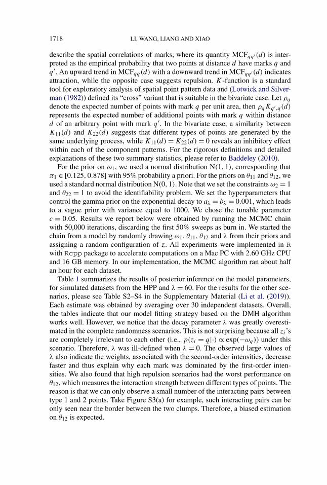
Since 1970s, there has been considerable interest in studying the spatial patternpresented by particular types of mammalian retinal cell bodies (Wässle, Peichl andBoycott (1981), Wässle and Riemann (1978), Hughes (1981a, 1981b), Peichl andWässle (1981), Rockhill, Euler and Masland (2000), Vaney, Peichl and Boycott(1981)). One of the two commonly used examples is the amacrine cells dataset(Diggle (1986)), consisting of two types of displaced amacrine cells within the reti-nal ganglion cell layer of a rabbit. The other is the betacells dataset (Wässleand Illing (1981)), composed of two types of beta cells that are associated with theresolution of fine details in the visual system of a cat. Figure 1 [left] and [middle]depict how the two different types of amacrine and beta cells distribute in restrictedrectangular regions. Their MCF and multitype k-function plots are shown in Fig-ure S5 in the supplemental material (Li et al. (2019)). Although the MCF plotsclearly indicate strong attraction among cells with the different type and the inter-action region radius around 0.1, no quantities can be accurately estimated further.We applied the proposed model with the same hyperparameter and algorithm set-tings as described in Section 4 and the choice of c = 0.2 for each dataset. Weran four independent MCMC chains and used the potential scale reduction factor(PSRF) (Gelman et al. (1992)) to evaluate convergence. PSRF is a statistic com-paring the estimated between-chains and within-chain variances for each modelparameter. Its value should be close to 1 if multiple chains have converged to thetarget posterior distribution. In this case, the PSRFs for all the model parameterswere below 1.029, clearly suggesting that the MCMC chains converged. Then, foreach dataset, we pooled together the outputs from the four chains and reported theestimated model parameters with their 95% credible interval in Figure S6 and S7.We plotted the estimated MIFs in Figure 2. Our method, as well as other methods(Diggle (1986), van Lieshout and Baddeley (1999)), suggest attraction between


FIG. 2. The MIF functions estimated from [left]: amacrine; [middle]: betacells; [right]:lansing (only the MIFs between the same mark are shown here; see Figure S8 for the numeri-cal results of interactions between different marks).

the cells (i.e., most cells have a nearest neighbor of the opposite type). The mes-sage about oppositely labeled pairs between neighbor cells would strengthen theassumption that there are two separate channels for brightness and darkness as pos-tulated by Hering in 1874. Furthermore, our method is able to provide an accuratequantitative description, which can benefit the development and retinal samplingefficiency.

The third dataset in spatstat that was used is the lansing dataset. It con-tains the locations and botanical classification of trees in a 924 × 924 feet (19.6acre) area of Lansing Woods, Clinton County, MI, USA. Figure 1 [right] shows therescaled multitype point pattern that consists of Q = 6 types of trees. The MCFplots are shown in Figure S5 in the Supplementary Material (Li et al. (2019)),which indicate exhibition of clustering among the trees with the same type. Withthe same hyperparameter, algorithm and convergence diagnostic settings, we ap-plied the proposed model with the choice of c = 0.1. The PSRFs were rangingfrom 1.003 to 1.022. The estimated model parameters are reported in Figure S8and the MIFs are summarized in Figure 2 [right]. The pattern reveals that the firstfive types of trees exhibited clustering, especially for black oak and miscellaneoustrees. This means if one species had a clump in an area, then no other speciestended to form a clump there. We also found white oak had the least φ̂qq value,which suggests its spatial pattern was more likely random. Those findings werealso reported in Cox and Lewis (1976) and Cox (1979). In addition, our MIF plotsindicates that there was no interaction between the same type trees beyond 90 feet.

5.2. Case study on lung cancer. Lung cancer is the leading cause of deathfrom cancer in both men and women. Non-small-cell lung cancer (NSCLC) ac-counts for about 85% of deaths from lung cancer. Current guidelines for diag-nosing and treating NSCLC are largely based on pathological examination ofH&E-stained tumor tissue section slides. We have developed a ConvPath pipeline(https://qbrc.swmed.edu/projects/cnn/) to determine the locations and types of

https://qbrc.swmed.edu/projects/cnn/


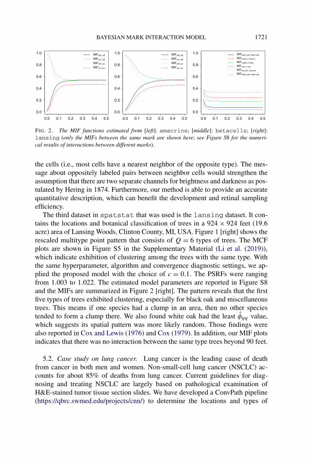
FIG. 3. Lung cancer case study: Two examples of the rescaled marked point data from NLSTdataset, where black, red and green points represent lymphocyte (◦), stromal (+) and tumor (�)cells. For the data shown in the left, λ̂ = 172.102, π̂lym = 0.022, π̂str = 0.173, π̂tum = 0.805

and φ̂tum,str = 0.012; For the data shown in the right, λ̂ = 169.268, π̂lym = 0.011, π̂str = 0.603,

π̂tum = 0.386 and φ̂tum,str = 0.162.

cells observed in the processed tumor pathology images. Specifically, the clas-sifier, based on a convolutional neural network (CNN), was trained using a largecohort of lung cancer pathology images manually labeled by pathologists, and itcan classify each cell by its Q = 3 category: lymphocyte (a type of immune cell),stromal, or tumor cell. The overall classification accuracy is 92.9% and 90.1% intraining and independent testing datasets, respectively (Wang et al. (2018)).

In this case study, we used the pathology images from 188 NSCLC patients inthe National Lung Screening Trial (NLST). Each patient has one or more tissueslide(s) scanned at 40× magnification. The median size of the slides is 24,244 ×19,261 pixels. A lung cancer pathologist first determined and labeled the region ofinterest (ROI) within the tumor region(s) from each tissue slide using an annotationtool, ImageScope (Leica Biosystem). ROIs are regions of the slides containing themajority of the malignant tissues and are representative of the whole slide image.Then we randomly chose five square regions, each of which is in a 5000 × 5000pixel window, per ROI as the sample images. The total number of sample imagesthat we collected was 1585. For each sample image, the ConvPath (illustrated inFigure S9 in the Supplementary Material (Li et al. (2019))) software was used toidentify cells from the sample images and classify each cell into one of three types,so that a corresponding spatial map of cells was generated and used as the inputof our model. The number of cells in each sample image ranges from n = 2876to 26,463. Figure 3 shows the examples of two sample images and Figure S10displays their MCF and multitype K-function plots.

We applied the proposed model with the same hyperparameter and algorithmsettings as described in Section 4 and different choices of c = 0.02, 0.05 and 0.1.We then computed the pairwise Pearson correlation coefficients between the esti-mated model parameters under different choices of c. These correlations indicated


TABLE 2Lung cancer case study: The p-values of the transformed model parameters (in percentile %) byfitting a Cox proportional hazards model with survival time (defined as the number of days fromdiagnosis to death for participants who died or last contact for all other participants) and vital

status (death or alive) as responses, and model parameters and clinical variables as predictors. Theoverall p-value (Wald test) is 0.003

Predictor Coefficient exp (Coef.) SE P -value

φ̂str,lym 0.147 1.158 0.052 0.106φ̂tum,lym 0.030 1.030 0.025 0.546φ̂lym,str −0.009 0.991 0.008 0.543φ̂tum,str 0.096 1.100 0.016 0.002φ̂lym,tum −0.002 0.998 0.008 0.896φ̂str,tum −0.059 0.943 0.019 0.128

π̂lym 0.034 1.035 0.015 0.219π̂str −0.032 0.969 0.007 0.019

λ̂ −0.006 0.994 0.003 0.382

Age 0.038 1.039 0.009 0.176

Female/male −0.138 0.871 0.091 0.631

Smoking/nonsmoking −0.001 0.999 0.089 0.997

substantial agreement between any pair of settings, with values ranging from 0.967to 0.997. The estimated parameters (with their summary statistics summarized inTable S5) that we used for the following three downstream analyses were obtainedunder the most conservative choice of c = 0.1.

5.2.1. Association study. With the estimated parameters in each sample im-age, we conducted a downstream analysis to investigate their associations with theother measurements of interest. Specifically, a Cox proportional hazards model(Cox (1992)) was fitted to evaluate the association between the transformed modelparameters π̂ and �̂ (in percentile %), and patient survival outcomes, after ad-justing for other clinical information, such as age, gender and tobacco history.Multiple sample images from the same patient were modeled as correlated obser-vations in the Cox proportional hazards model to compute a robust variance foreach coefficient. The overall p-value for the Cox model was 0.002 (Wald test), andthe p-value and coefficient for each individual variable are summarized in Table 2.The results imply that a low interaction between stromal and tumor cells is asso-ciated with good prognosis in NSCLC patients (p-value = 0.007). Interestingly,Beck et al. (2011) also discovered that the morphological features of the stromain the tumor region are associated with patient survival in a systematic analysis ofbreast cancer. Besides, the abundance of the stromal cells itself (p-value = 0.017)is also a prognostic factor, while the underlying biological mechanism is currently


unknown. The positive coefficient of the predictor φtum,str implies that a highervalue may reveal a higher risk of death. Indeed, we obtained φ̂tum,str = 0.012 forthe data shown in Figure 3 [left] and it was from a patient who was still alive over2615 days after the surgery, while the estimated value of φtum,str = 0.162 for thedata shown in Figure 3 [right] and it was from a patient who died on the 1246th dayafter the surgery. These two images have distinctive patterns, as the former clearlyshows the same type cells tend to clump in the same area, while the latter displaysa case where stromal and tumor cells are thoroughly mixed together, indicating thespread of stromal cells into the tumor region. Although the high/low interactionbetween stromal and tumor cells can be easily seen by eyes in these two images,the patterns are much more subtle for many other images. Therefore, the proposedmodel can be used to predict the survival time when human visualization does notwork.

By contrast, we fitted a similar Cox proportional hazards model by us-ing the MCF features as predictors. Specifically, we first used MCFlym,lym(d),MCFlym,str(d), MCFlym,tum(d), MCFstr,str(d) and MCFstr,tum(d), where d = 0.1for each sample image as covariates. The results are summarized in Table S6 in theSupplementary Material (Li et al. (2019)). As we can see, there was no significantpredictor and the overall p-value for the Cox model was 0.60 (Wald test). Next, wetried to vary d from 0 to 0.1. Figure S12(a) shows the p-values of those statisticsagainst d . We repeated this analysis with the features from multitype K-functionsand reported the results in Table S7 and Figure S12(b). Again, we were unableto find any association between cell–cell interactions and clinical outcomes. Thecomparison demonstrates the advantage of modeling the pathology images via theproposed model over the traditional explanatory analysis for characterizing spatialcorrelation.

5.2.2. Predictive performance by cross-validation. Lastly, we used leave-one-out cross-validation to evaluate the above Cox proportional hazards model. Specif-ically, we trained the model by using (N − 1) sample images and then predictedthe risk score of the left-out sample. After repeating this step for each of the N

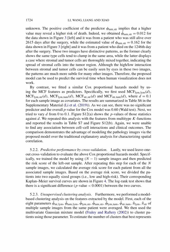
sample images, we calculated the average risk score for each patient from all theassociated sample images. Based on the average risk score, we divided the pa-tients into two equally sized groups (i.e., low and high-risk). Their correspondingKaplan–Meier survival curves are shown in Figure 4. The log-rank test shows thatthere is a significant difference (p-value < 0.0001) between the two curves.

5.2.3. Unsupervised clustering analysis. Furthermore, we performed a model-based clustering analysis on the features extracted by the model. First, each of theeight parameters φ̂str,lym, φ̂tum,lym, φ̂lym,str, φ̂tum,str, φ̂lym,tum, φ̂str,tum, π̂lym, π̂str ofmultiple sample images from the same patient were averaged. We then used themultivariate Gaussian mixture model (Fraley and Raftery (2002)) to cluster pa-tients using those parameter. To estimate the number of clusters that best represents


FIG. 4. Lung cancer case study: The Kaplan–Meier plot for the low and high-risk groups obtainedby leave-one-out cross-validation (log rank test p-value < 0.0001).

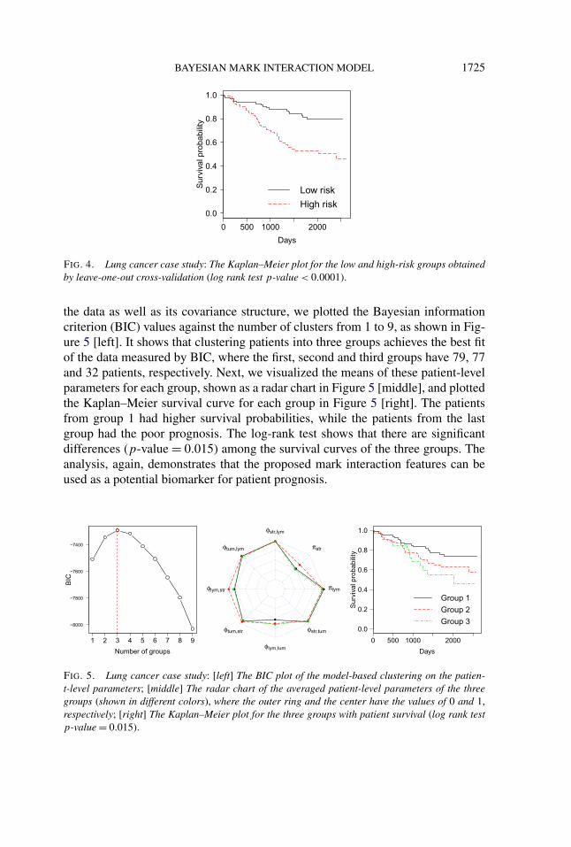
the data as well as its covariance structure, we plotted the Bayesian informationcriterion (BIC) values against the number of clusters from 1 to 9, as shown in Fig-ure 5 [left]. It shows that clustering patients into three groups achieves the best fitof the data measured by BIC, where the first, second and third groups have 79, 77and 32 patients, respectively. Next, we visualized the means of these patient-levelparameters for each group, shown as a radar chart in Figure 5 [middle], and plottedthe Kaplan–Meier survival curve for each group in Figure 5 [right]. The patientsfrom group 1 had higher survival probabilities, while the patients from the lastgroup had the poor prognosis. The log-rank test shows that there are significantdifferences (p-value = 0.015) among the survival curves of the three groups. Theanalysis, again, demonstrates that the proposed mark interaction features can beused as a potential biomarker for patient prognosis.

FIG. 5. Lung cancer case study: [left] The BIC plot of the model-based clustering on the patien-t-level parameters; [middle] The radar chart of the averaged patient-level parameters of the threegroups (shown in different colors), where the outer ring and the center have the values of 0 and 1,respectively; [right] The Kaplan–Meier plot for the three groups with patient survival (log rank testp-value = 0.015).


6. Conclusion. The major cell types in a malignant tissue of lung are tumorcells, stromal cells and infiltrating lymphocytes. The distribution of different typesof cells and their interactions play a key role in tumor progression and metasta-sis. For example, stromal cells are connective tissue cells, such as fibroblasts andpericytes, and their interaction with tumor cells is known to play a major role incancer progression (Wiseman and Werb (2002)). Tumor-infiltrating lymphocyteshave been associated with patient prognosis in multiple tumor types previously(Brambilla et al. (2016), Huh, Lee and Kim (2012)). Recent advances in deeplearning methods have made possible the automatic identification and classifica-tion of cells at large scale. For example, the ConvPath pipeline could determine thelocation and cell type for thousands of cells. However, it is challenging to utilizethe vast amount of information extracted digitally. In this study, we developed aBayesian statistical method to model the spatial interaction among different typesof cells in tumor regions. We focused on modeling the spatial correlation of marksin a spatial pattern that arose from a pathology image study. A Bayesian frame-work was proposed in order to model how the mark in a pattern might have beenformed given the points. The proposed model can utilize the spatial informationof thousands of points from any point processes. The output of the model is theparameters that characterize the spatial pattern. After a certain transformation, theparameters are identifiable and interpretable, and most importantly, transferable forconducting an association study with other measurements of interest. Furthermore,this statistical methodology provides new insights into the biological mechanismsof cancer.

For the lung cancer pathology imaging data, our study shows the interactionstrength between stromal and tumor cells is associated with patient prognosis.This parameter can be easily measured using the proposed method and used asa potential biomarker for patient prognosis. This biomarker can be translated intoreal clinical tools at low cost because it is based only on tumor pathology slides,which are available in standard clinical care.

Several extensions of our model are worth investigating. First, the proposedmodel can be extended to finite mixture models for inhomogeneous mark interac-tions. Second, the correlation among first- and second-order intensity parameterscould be taken into account by modeling them as a multivariate normal distribu-tion. Third, in some scenarios, we may need to consider edge effects in that themarks associated with the points within the observation window may also interactwith those marks of points outside the window. Therefore, some edge-correctionmethods, such as minus sampling, should be employed. Last but not least, theproposed model provides a good chance to investigate the performance of otherapproximate Bayesian computation methods, such as variational Bayes (Ren et al.(2011)). These could be future research directions.


APPENDIX: MCMC ALGORITHM

Update of ω: We update each of ωq, q = 1, . . . ,Q − 1 by using the DMH al-gorithm. We first propose a new ω∗

q from N(ωq, τ2ω). Next, according to equation

(2.5), we implement the Gibbs sampler to simulate an auxiliary variable z∗ startingfrom z based on the new ω∗, where all the elements are the same as ω excludingthe qth one. The proposed value ω∗

q is then accepted to replace the old value withprobability min(1, r). The Hastings ratio r is given as

r = p(z∗|ω,�, λ)

p(z|ω,�, λ)

p(z|ω∗,�, λ)

p(z∗|ω∗,�, λ)

N(ω∗q;μω,σ 2

ω)

N(ωq;μω,σ 2ω)

J (ωq;ω∗q)

J (ω∗q;ωq)

,

where the form of p(z|ω,�, λ) is given by equation (2.4). As a result, the nor-malizing constant in equation (2.4) can be canceled out. Note that the last fractionterm, which is the proposal density ratio, equals 1 for this random walk Metropolisupdate on ωq .

Update of �: We update each of θqq ′, q = 1, . . . ,Q−1, q ′ = q, . . . ,Q by usingthe DMH algorithm. We first propose a new θ∗

qq ′ from N(θqq ′, τ 2θ ) and set θ∗

q ′q =θ∗qq ′ as the matrix is symmetric. Next, according to equation (2.5), an auxiliary

variable z∗ is simulated via the Gibbs sampler with z as the starting point. Thissimulation should be based on the new �∗, where all the elements are the same as� except the two elements corresponding to θqq ′ and θq ′q . The proposed value θ∗

qq ′as well as θ∗

q ′q is then accepted to replace the old values with probability min(1, r).The Hastings ratio r is given as

r = p(z∗|ω,�, λ)

p(z|ω,�, λ)

p(z|ω,�∗, λ)

p(z∗|ω,�∗, λ)

N(θ∗qq ′ ;μθ,σ

2θ )

N(θqq ′ ;μθ,σ2θ )

J (θqq ′ ; θ∗qq ′)

J (θ∗qq ′ ; θqq ′)

,

where the form of Pr(z|θ , λ) is given by equation (2.4). As a result, the normaliz-ing constant in equation (2.4) can be canceled out. Note that the last fraction term,which is the proposal density ratio, equals 1 for this random walk Metropolis up-date on θqq ′ .

Update of λ: We update the decay parameter λ by using the DMH algorithm.We first propose a new λ∗ from a gamma distribution Ga(λ2/τλ, λ/τλ), where themean is λ and the variance is τλ. Next, according to equation (2.5), we implementthe Gibbs sampler to simulate an auxiliary variable z∗ starting from z based onthe new λ∗. The proposed value λ∗ is then accepted to replace the old value withprobability min(1, r). The Hastings ratio r is given as

r = p(z∗|ω,�, λ)

p(z|ω,�, λ)

p(z|ω,�, λ∗)p(z∗|ω,�, λ∗)

Ga(λ∗;a, b)

Ga(λ;a, b)

J (λ;λ∗)J (λ∗;λ)

,

where the form of Pr(z|θ , λ) is given by equation (2.4). As a result, the normaliz-ing constant in equation (2.4) can be canceled out. Note that the last fraction term,which is the proposal density ratio, equals 1 for this random walk Metropolis up-date on λ.


Acknowledgment. The authors would like to thank Jessie Norris for helpingus in proofreading the manuscript.

SUPPLEMENTARY MATERIAL

Figures and tables (DOI: 10.1214/19-AOAS1254SUPPA; .pdf). We provideadditional supporting plots and tables.

Code (DOI: 10.1214/19-AOAS1254SUPPB; .zip). We provide code in the formof R/C++ code. It can also be downloaded from GitHub (link: https://github.com/liqiwei2000/BayesMarkInteractionModel).

REFERENCES

AMIN, M. B., TAMBOLI, P., MERCHANT, S. H., ORDÓÑEZ, N. G., RO, J., AYALA, A. G. andRO, J. Y. (2002). Micropapillary component in lung adenocarcinoma: A distinctive histologicfeature with possible prognostic significance. Amer. J. Surg. Pathol. 26 358–364.

AVALOS, G. and BUCCI, F. (2014). Exponential decay properties of a mathematical model for acertain fluid-structure interaction. In New Prospects in Direct, Inverse and Control Problems forEvolution Equations. Springer INdAM Ser. 10 49–78. Springer, Cham. MR3362986

BADDELEY, A. (2010). Multivariate and marked point processes. In Handbook of Spatial Statistics(A. E. Gelfand, P. Diggle, P. Guttorp and M. Fuentes, eds.). Chapman & Hall/CRC Handb. Mod.Stat. Methods 371–402. CRC Press, Boca Raton, FL. MR2730956

BADDELEY, A. and TURNER, R. (2006). Modelling spatial point patterns in R. In Case Studies inSpatial Point Process Modeling. Lect. Notes Stat. 185 23–74. Springer, New York. MR2232122

BARLETTA, J. A., YEAP, B. Y. and CHIRIEAC, L. R. (2010). Prognostic significance of grading inlung adenocarcinoma. Cancer 116 659–669.

BECK, A. H., SANGOI, A. R., LEUNG, S., MARINELLI, R. J., NIELSEN, T. O., VAN DE VI-JVER, M. J., WEST, R. B., VAN DE RIJN, M. and KOLLER, D. (2011). Systematic analysis ofbreast cancer morphology uncovers stromal features associated with survival. Sci. TranslationalMed. 3 108–113.

BESAG, J. E. (1977). Comment on “Modelling spatial patterns.” J. Roy. Statist. Soc. Ser. B 39 193–195.

BOGNAR, M. A. (2008). Bayesian modeling of continuously marked spatial point patterns. Comput.Statist. 23 361–379. MR2425167

BORCZUK, A. C., QIAN, F., KAZEROS, A., ELEAZAR, J., ASSAAD, A., SONETT, J. R., GINS-BURG, M., GORENSTEIN, L. and POWELL, C. A. (2009). Invasive size is an independent pre-dictor of survival in pulmonary adenocarcinoma. Amer. J. Surg. Pathol. 33 462.

BRAMBILLA, E., LE TEUFF, G., MARGUET, S., LANTUEJOUL, S., DUNANT, A., GRAZIANO, S.,PIRKER, R., DOUILLARD, J.-Y., LE CHEVALIER, T., FILIPITS, M. et al. (2016). Prognosticeffect of tumor lymphocytic infiltration in resectable non-small-cell lung cancer. J. Clin. Oncol.34 1223–1230.

CARPENTER, A. E., JONES, T. R., LAMPRECHT, M. R., CLARKE, C., KANG, I. H., FRIMAN, O.,GUERTIN, D. A., CHANG, J. H., LINDQUIST, R. A., MOFFAT, J. et al. (2006). CellProfiler:Image analysis software for identifying and quantifying cell phenotypes. Genome Biol. 7 R100.

CHULAEVSKY, V. (2014). Exponential decay of eigenfunctions in a continuous multi-particle An-derson model with sub-exponentially decaying interaction. Available at arXiv:1408.4646.

COX, T. F. (1979). A method for mapping the dense and sparse regions of a forest stand. Appl.Statist. 28 14–19.

https://doi.org/10.1214/19-AOAS1254SUPPA

https://doi.org/10.1214/19-AOAS1254SUPPB

https://github.com/liqiwei2000/BayesMarkInteractionModel

http://www.ams.org/mathscinet-getitem?mr=3362986




http://arxiv.org/abs/arXiv:1408.4646

https://github.com/liqiwei2000/BayesMarkInteractionModel


COX, D. R. (1992). Regression models and life-tables In Breakthroughs in Statistics, Vol. II. Method-ology and Distribution (S. Kotz and N. L. Johnson, eds.) 527–541. Springer, Berlin.

COX, T. F. and LEWIS, T. (1976). A conditioned distance ratio method for analyzing spatial patterns.Biometrika 63 483–491. MR0445713

DALE, M. R. (2000). Spatial Pattern Analysis in Plant Ecology. Cambridge Univ. Press, Cambridge.DIGGLE, P. J. (1986). Displaced amacrine cells in the retina of a rabbit: Analysis of a bivariate

spatial point pattern. J. Neuroscience Methods 18 115–125.DIGGLE, P. J. and COX, T. (1981). On sparse sampling methods and tests of independence for

multivariate spatial point patterns. Bulletin Internat. Statist. Inst. 49 213–229.DIGGLE, P. J., EGLEN, S. J. and TROY, J. B. (2006). Modelling the bivariate spatial distribution of

amacrine cells. In Case Studies in Spatial Point Process Modeling. Lect. Notes Stat. 185 215–233.Springer, New York. MR2232131

DIGGLE, P. J. and MILNE, R. K. (1983). Bivariate Cox processes: Some models for bivariate spatialpoint patterns. J. Roy. Statist. Soc. Ser. B 45 11–21. MR0701070

FRALEY, C. and RAFTERY, A. E. (2002). Model-based clustering, discriminant analysis, and densityestimation. J. Amer. Statist. Assoc. 97 611–631. MR1951635

GELFAND, A. E., DIGGLE, P., GUTTORP, P. and FUENTES, M. (2010). Handbook of Spatial Statis-tics. CRC Press, Boca Raton, FL.

GELMAN, A., RUBIN, D. B. (1992). Inference from iterative simulation using multiple sequences.Statist. Sci. 7 457–472.

GELMAN, A., CARLIN, J. B., STERN, H. S., DUNSON, D. B., VEHTARI, A. and RUBIN, D. B.(2014). Bayesian Data Analysis, 3rd ed. Texts in Statistical Science Series. CRC Press, BocaRaton, FL. MR3235677

GILLIES, R. J., VERDUZCO, D. and GATENBY, R. A. (2012). Evolutionary dynamics of carcino-genesis and why targeted therapy does not work. Nat. Rev. Cancer 12 487–493.

GLEASON, D. F. and MELLINGER, G. T. (2002). Prediction of prognosis for prostatic adenocarci-noma by combined histological grading and clinical staging. J. Urology 167 953–958.

GRABARNIK, P., MYLLYMÄKI, M. and STOYAN, D. (2011). Correct testing of mark independencefor marked point patterns. Ecol. Model. 222 3888–3894.

HAMMERSLEY, J. M. and CLIFFORD, P. (1971). Markov fields on finite graphs and lattices.HANAHAN, D. and WEINBERG, R. A. (2011). Hallmarks of cancer: The next generation. Cell 144

646–674.HUGHES, A. (1981a). Cat retina and the sampling theorem: The relation of transient and sustained

brisk-unit cut-off frequency to α and β-mode cell density. Experimental Brain Res. 42 196–202.HUGHES, A. (1981b). Population magnitudes and distribution of the major modal classes of cat

retinal ganglion cell as estimated from HRP filling and a systematic survey of the soma diameterspectra for classical neurones. J. Comparative Neurology 197 303–339.

HUH, J. W., LEE, J. H. and KIM, H. R. (2012). Prognostic significance of tumor-infiltrating lym-phocytes for patients with colorectal cancer. Archives of Surgery 147 366–372.

HUI, E. E. and BHATIA, S. N. (2007). Micromechanical control of cell–cell interactions. Proc.Natn. Acad. Sci. 104 5722–5726.

ILLIAN, J., PENTTINEN, A., STOYAN, H. and STOYAN, D. (2008). Statistical Analysis and Mod-elling of Spatial Point Patterns. Statistics in Practice. Wiley, Chichester. MR2384630

JUNTTILA, M. R. and DE SAUVAGE, F. J. (2013). Influence of tumour micro-environment hetero-geneity on therapeutic response. Nature 501 346–354.

KAMENTSKY, L., JONES, T. R., FRASER, A., BRAY, M.-A., LOGAN, D. J., MADDEN, K. L.,LJOSA, V., RUEDEN, C., ELICEIRI, K. W. and CARPENTER, A. E. (2011). Improved structure,function and compatibility for CellProfiler: Modular high-throughput image analysis software.Bioinformatics 27 1179–1180.

KASHIMA, Y. (2010). Exponential decay of correlation functions in many-electron systems. J. Math.Phys. 51 063521, 40. MR2676498









LI, Q., YI, F., WANG, T., XIAO, G. and LIANG, F. (2017). Lung cancer pathological image analysisusing a hidden Potts model. Cancer Informatics 16 1176935117711910.

LI, Q., WANG, X., LIANG, F. and XIAO, G. (2019). Supplement to “A Bayesian mark inter-action model for analysis of tumor pathology images.” DOI:10.1214/19-AOAS1254SUPPA,DOI:10.1214/19-AOAS1254SUPPB.

LIANG, F. (2010). A double Metropolis–Hastings sampler for spatial models with intractable nor-malizing constants. J. Stat. Comput. Simul. 80 1007–1022. MR2742519

LIANG, F., JIN, I. H., SONG, Q. and LIU, J. S. (2016). An adaptive exchange algorithm for samplingfrom distributions with intractable normalizing constants. J. Amer. Statist. Assoc. 111 377–393.MR3494666

LOTWICK, H. W. and SILVERMAN, B. W. (1982). Methods for analysing spatial processes of severaltypes of points. J. Roy. Statist. Soc. Ser. B 44 406–413. MR0693241

LUO, X., ZANG, X., YANG, L., HUANG, J., LIANG, F., CANALES, J. R., WISTUBA, I. I., GAZ-DAR, A., XIE, Y. and XIAO, G. (2016). Comprehensive computational pathological image anal-ysis predicts lung cancer prognosis. J. Thorac. Oncol. DOI:10.1016/j.jtho.2016.10.017.

MANTOVANI, A., SOZZANI, S., LOCATI, M., ALLAVENA, P. and SICA, A. (2002). Macrophagepolarization: Tumor-associated macrophages as a paradigm for polarized M2 mononuclear phago-cytes. Trends in Immunology 23 549–555.

MATTFELDT, T., ECKEL, S., FLEISCHER, F. and SCHMIDT, V. (2009). Statistical analysis of la-belling patterns of mammary carcinoma cell nuclei on histological sections. J. Microsc. 235 106–118. MR2731112

MERLO, L. M., PEPPER, J. W., REID, B. J. and MALEY, C. C. (2006). Cancer as an evolutionaryand ecological process. Nat. Rev. Cancer 6 924–935.

MØLLER, J., PETTITT, A. N., REEVES, R. and BERTHELSEN, K. K. (2006). An efficient Markovchain Monte Carlo method for distributions with intractable normalising constants. Biometrika93 451–458. MR2278096

MURRAY, I., GHAHRAMANI, Z. and MACKAY, D. (2012). MCMC for doubly-intractable distribu-tions. Available at arXiv:1206.6848.

OGATA, Y. and TANEMURA, M. (1985). Estimation of interaction potentials of marked spatial pointpatterns through the maximum likelihood method. Biometrics 41 421–433.

ORIMO, A., GUPTA, P. B., SGROI, D. C., ARENZANA-SEISDEDOS, F., DELAUNAY, T.,NAEEM, R., CAREY, V. J., RICHARDSON, A. L. and WEINBERG, R. A. (2005). Stromal fi-broblasts present in invasive human breast carcinomas promote tumor growth and angiogenesisthrough elevated SDF-1/CXCL12 secretion. Cell 121 335–348.

PEICHL, L. and WÄSSLE, H. (1981). Morphological identification of on-and off-centre brisk tran-sient (Y) cells in the cat retina. Proc. Roy. Soc. London Ser. B, Biolog. Sci. 212 139–153.

PENROSE, O. and LEBOWITZ, J. L. (1974). On the exponential decay of correlation functions.Comm. Math. Phys. 39 165–184. MR0432092

POLYAK, K., HAVIV, I. and CAMPBELL, I. G. (2009). Co-evolution of tumor cells and their mi-croenvironment. Trends Genet. 25 30–38.

REN, Q., BANERJEE, S., FINLEY, A. O. and HODGES, J. S. (2011). Variational Bayesian methodsfor spatial data analysis. Comput. Statist. Data Anal. 55 3197–3217. MR2825404

RINCÓN, J., GANAHL, M. and VIDAL, G. (2015). Lieb–Liniger model with exponentially decayinginteractions: A continuous matrix product state study. Phys. Rev. B 92 115107.

RIPLEY, B. D. (1977). Modelling spatial patterns. J. Roy. Statist. Soc. Ser. B 39 172–212.MR0488279

ROCKHILL, R. L., EULER, T. and MASLAND, R. H. (2000). Spatial order within but not betweentypes of retinal neurons. Proc. Natn. Acad. Sci. 97 2303–2307.

SABO, E., BECK, A. H., MONTGOMERY, E. A., BHATTACHARYA, B., MEITNER, P., WANG, J. Y.and RESNICK, M. B. (2006). Computerized morphometry as an aid in determining the grade ofdysplasia and progression to adenocarcinoma in Barrett’s esophagus. Lab. Investigation 86 1261.

https://doi.org/10.1214/19-AOAS1254SUPPA

https://doi.org/10.1214/19-AOAS1254SUPPB




https://doi.org/10.1016/j.jtho.2016.10.017








SEGAL, D. M. and STEPHANY, D. A. (1984). The measurement of specific cell: Cell interactionsby dual-parameter flow cytometry. Cytometry A 5 169–181.

SERTEL, O., KONG, J., CATALYUREK, U. V., LOZANSKI, G., SALTZ, J. H. and GURCAN, M. N.(2009a). Histopathological image analysis using model-based intermediate representations andcolor texture: Follicular lymphoma grading. J. Signal Processing Systems 55 169.

SERTEL, O., KONG, J., SHIMADA, H., CATALYUREK, U. V., SALTZ, J. H. and GURCAN, M. N.(2009b). Computer-aided prognosis of neuroblastoma on whole-slide images: Classification ofstromal development. Pattern Recognit. 42 1093–1103.

STOYAN, D. and PENTTINEN, A. (2000). Recent applications of point process methods in forestrystatistics. Statist. Sci. 15 61–78. MR1842237

TABESH, A., TEVEROVSKIY, M., PANG, H.-Y., KUMAR, V. P., VERBEL, D., KOTSIANTI, A. andSAIDI, O. (2007). Multifeature prostate cancer diagnosis and Gleason grading of histologicalimages. IEEE Trans. Med. Imag. 26 1366–1378.

TSAO, M.-S., MARGUET, S., LE TEUFF, G., LANTUEJOUL, S., SHEPHERD, F. A., SEYMOUR, L.,KRATZKE, R., GRAZIANO, S. L., POPPER, H. H., ROSELL, R. et al. (2015). Subtype classifica-tion of lung adenocarcinoma predicts benefit from adjuvant chemotherapy in patients undergoingcomplete resection. J. Clin. Oncol. 33 3439–3446.

VAN LIESHOUT, M. N. M. and BADDELEY, A. J. (1996). A nonparametric measure of spatialinteraction in point patterns. Stat. Neerl. 50 344–361. MR1422574

VAN LIESHOUT, M. N. M. and BADDELEY, A. J. (1999). Indices of dependence between types inmultivariate point patterns. Scand. J. Stat. 26 511–532. MR1734259

VANEY, D. I., PEICHL, L. and BOYCOTT, B. (1981). Matching populations of amacrine cells inthe inner nuclear and ganglion cell layers of the rabbit retina. J. Comparative Neurology 199373–391.

VINCENT, L. and JEULIN, D. (1989). Minimal paths and crack propagation simulations. Acta Stere-ologica 8 487–494.

WALLER, L. A. (2005). Bayesian thinking in spatial statistics. In Bayesian Thinking: Model-ing and Computation. Handbook of Statist. 25 589–622. Elsevier/North-Holland, Amsterdam.MR2490540

WANG, S., WANG, T., YANG, L., YI, F., LUO, X., YANG, Y., GAZDAR, A., FUJIMOTO, J.,WISTUBA, I. I., YAO, B. et al. (2018). ConvPath: A software tool for lung adenocarci-noma digital pathological image analysis aided by convolutional neural network. Available atarXiv:1809.10240.

WÄSSLE, H. and ILLING, R.-B. (1981). Morphology and mosaic of on-and off-beta cells in thecat retina and some functional considerations. Proc. Roy. Soc. London Ser. B, Biolog. Sci. 212177–195.

WÄSSLE, H., PEICHL, L. and BOYCOTT, B. B. (1981). Dendritic territories of cat retinal ganglioncells. Nature 292 344–345.

WÄSSLE, H. and RIEMANN, H. (1978). The mosaic of nerve cells in the mammalian retina. Proc.Roy. Soc. London Ser. B, Biolog. Sci. 200 441–461.

WIEGAND, T. and MOLONEY, K. A. (2004). Rings, circles, and null-models for point pattern anal-ysis in ecology. Oikos 104 209–229.

WISEMAN, B. S. and WERB, Z. (2002). Stromal effects on mammary gland development and breastcancer. Science 296 1046–1049.

XIAO, G., REILLY, C. and KHODURSKY, A. B. (2009). Improved detection of differentially ex-pressed genes through incorporation of gene locations. Biometrics 65 805–814. MR2649853

XIAO, G., WANG, X. and KHODURSKY, A. B. (2011). Modeling three-dimensional chromosomestructures using gene expression data. J. Amer. Statist. Assoc. 106 61–72. MR2816702

YU, K.-H., ZHANG, C., BERRY, G. J., ALTMAN, R. B., RÉ, C., RUBIN, D. L. and SNYDER, M.(2016). Predicting non-small cell lung cancer prognosis by fully automated microscopic pathol-ogy image features. Nat. Commun. 7.









YUAN, Y., FAILMEZGER, H., RUEDA, O. M., ALI, H. R., GRÄF, S., CHIN, S.-F.,SCHWARZ, R. F., CURTIS, C., DUNNING, M. J., BARDWELL, H. et al. (2012). Quantitativeimage analysis of cellular heterogeneity in breast tumors complements genomic profiling. Sci.Translational Med. 4 157ra143.

Q. LI

DEPARTMENT OF MATHEMATICAL SCIENCES

UNIVERSITY OF TEXAS AT DALLAS

FOUNDERS BUILDING FO 2.604D800 WEST CAMPBELL RD

RICHARDSON, TEXAS 75080USAE-MAIL: [email protected]: https://sites.google.com/site/liqiwei2000

X. WANG

DEPARTMENT OF STATISTICAL SCIENCE

SOUTHERN METHODIST UNIVERSITY

HEROY SCIENCE HALL 1023225 DANIEL AVE

DALLAS, TEXAS 75275USAE-MAIL: [email protected]: http://faculty.smu.edu/swang/

F. LIANG

DEPARTMENT OF STATISTICS

PURDUE UNIVERSITY

MATH BUILDING 520250 N. UNIVERSITY ST

WEST LAFAYETTE, INDIANA 47907USAE-MAIL: [email protected]: http://www.stat.purdue.edu/~fmliang/

G. XIAO

DEPARTMENT OF POPULATION

AND DATA SCIENCES

UNIVERSITY OF TEXAS

SOUTHWESTERN MEDICAL CENTER

DANCIGER BUILDING H9.1245323 HARRY HLINES BLVD

DALLAS, TEXAS 75390USAURL: https://sites.google.com/site/liqiwei2000https://qbrc.swmed.edu/labs/xiaolab

mailto:[email protected]

https://sites.google.com/site/liqiwei2000


http://faculty.smu.edu/swang/


http://www.stat.purdue.edu/~fmliang/

https://sites.google.com/site/liqiwei2000

https://qbrc.swmed.edu/labs/xiaolab

a bayesian mark interaction model for analysis of tumor

Documents