a bayesian spatial and temporal modeling … an examination of spatio-temporal variation in less...

1Division of Research Methodology, National Center for Health Statistics, Centers for Disease Control and Prevention, Hyattsville, MD 207822

2 Division of Vital Statistics, National Center for Health Statistics, Centers for Disease Control and Prevention, Hyattsville, MD 20782

3 Office of Analysis and Epidemiology, National Center for Health Statistics, Centers for Disease Control and Prevention, Hyattsville, MD 20782

Abstract: Hierarchical Bayes models have been used in disease mapping to examine

small scale geographic variation. State level geographic variation for less common

causes of mortality outcomes have been reported however county level variation is rarely

examined. Due to concerns about statistical reliability and confidentiality, county-level

mortality rates based on fewer than 20 deaths are suppressed based on Division of Vital

Statistics, National Center for Health Statistics (NCHS) statistical reliability criteria,

precluding an examination of spatio-temporal variation in less common causes of

mortality outcomes such as suicide rates (SRs) at the county level using direct estimates.

Existing Bayesian spatio-temporal modeling strategies can be applied via Integrated

Nested Laplace Approximation (INLA) in R to a large number of rare causes of mortality

outcomes to enable examination of spatio-temporal variations on smaller geographic

scales such as counties. This method allows examination of spatiotemporal variation

across the entire U.S., even where the data are sparse. We used mortality data from 2005-

2015 to explore spatiotemporal variation in SRs, as one particular application of the

Bayesian spatio-temporal modeling strategy in R-INLA to predict year and county-

specific SRs. Specifically, hierarchical Bayesian spatio-temporal models were

implemented with spatially structured and unstructured random effects, correlated time

effects, time varying confounders and space-time interaction terms in the software R-

INLA, borrowing strength across both counties and years to produce smoothed county

level SRs. Model-based estimates of SRs were mapped to explore geographic variation.

Running head: Mapping Geographic Variation in Mortality Rates

Key words: Hierarchical Bayes, Integrated Nested Laplace Approximation, Small area

estimation, Suicide rates

1. Introduction and motivation

The use of Bayesian methods in the areas of disease mapping, epidemiology, and small area health

applications is well established. The Bayesian inference combines the prior distribution on model

parameters and the data likelihood to derive the posterior distribution which summarizes the behavior

of the parameters in light of the observed data. (Lawson, A. (2013)) Bayesian hierarchical models that

incorporate time and area effects provide additional insights in terms of the interpretability and

similarity based on the neighborhood structure of areas and adjacent times. However, incorporating

time and area effects results in increasingly complex model structures which can substantially increase

the computational time required to estimate these models.

Journal of Data Science 18(2018), 147-182

A BAYESIAN SPATIAL AND TEMPORAL MODELING APPROACH TO

MAPPING GEOGRAPHIC VARIATION IN MORTALITY RATES FOR

SUBNATIONAL AREAS WITH R-INLA

Diba Khana1, Lauren M. Rossen 2, Holly Hedegaard 3, Margaret Warner 4

Traditionally, Markov Chain Monte Carlo (MCMC methods) have been used to approximate the

posterior marginals in Bayesian Hierarchical models and are computationally intensive and time

consuming. Two basic methods, namely, Gibbs sampling and Metropolis-Hastings are designed in

Winbugs software (Ntzoufras, I. (2009)) to approximate the posterior distributions via MCMC. The

computation time in reaching convergence for the different parameters in the model can often be

measured in days or weeks of time for big datasets or large models. (Barker, L. E. et al. (2013), Bivand,

R.S. et. al. (2015), Khan, D. et. al. (2018), Martins, T.G. et al. (2013), Rue, H. et al. (2009), Rue, H.

and Martino, S. (2009)) Further, the highly multivariate structure of the models limits the ability to

approximate the full posterior distributions. Several other packages exist for example, STAN (Stan

Development Team (2016)) but require a certain level of programming expertise. Spatial models are

not built-in in JAGS (Plummer, M. (2003)) and hence need to be programmed.

The INLA method has been introduced as an alternative to MCMC to approximate the posterior

marginals of latent Gaussian models and significantly reduces the computation time. (Rue, H. et.al.

(2009) The INLA method does not use iterative computation techniques like MCMC. The posterior

approximation is achieved by applying numerical integrations for fixed effects and Laplace integral

approximation to the random effects (Chen, C. et al. (2014), Martins, T.G. et al. (2013), Rue, H. et al.

(2009), Rue, H. and Martino, S. (2009)). Models are built-in and can be fitted in R-INLA, using R

commands (Bivand, R. S. (2015))

In this study, we examine existing Bayesian spatio-temporal models in the software R-INLA for

the purposes of mapping less common causes of mortality outcomes on small geographic scales and

consider suicide rates (SRs) at the county level as one particular application. Mapping county level

estimates provides greater understanding of the trends and variability in spatio-temporal patterns of

less common causes of mortality outcomes not possible by examination of direct national and state

estimates (Schaible, W.L. (1996)) or by examination of direct county level estimates. Additionally,

mapping county-level estimates can help highlight areas where estimates are higher or lower than the

national average, and provide additional insights on how county-level estimates have changed over

time across the U.S. Due to the potential instability of the direct estimates of less common causes of

mortality outcomes at smaller geographic scales such as counties, compounded by small population

sizes, the annual county level direct estimates are typically not reported. For example, the majority of

counties across the U.S. report fewer than 20 suicide deaths in any given year, the criterion for

suppression of death rates due to concerns about statistical reliability by the Division of Vital Statistics

at the National Center for Health Statistics. (Kochanek, K.D. et al. (2016), page 118) To account for

the problems encountered in examining spatio-temporal variations with county level direct estimates

for less common causes of mortality outcomes such as SRs over time, as outlined above, we propose

to examine existing hierarchical Bayesian spatio-temporal models that account for extra uncertainty,

inherent spatial autocorrelation, and the time dependent structure of the data to produce smoothed

model based yearly county level SRs in the software R-INLA to examine broad scale trend and

variability in spatiotemporal patterns in SRs across 3,140 U.S. counties from 2005 through 2015.

(Knorr-Held, L. and Besag, J. (1998), Lawson, A. (2013), Lawson, A. (2015), Lagazio, C. et al. (2001),

Wall, M. M. (2004), Xia, H., et al. (1997))

Specifically, in a Bayesian spatio-temporal model, the spatially structured and unstructured random

effects are used to model the inherent spatial autocorrelation in the data, the correlated and uncorrelated

time effects model the time dependent structure of the data, time varying covariates model the extra

uncertainty in the data due to measured confounders, and the space-time interaction effects model the

148 A BAYESIAN SPATIAL AND TEMPORAL MODELING APPROACH TO MAPPING GEOGRAPHIC VARIATION IN MORTALITY RATES FOR SUBNATIONAL AREAS WITH R-INLA

residual spatio-temporal variation that are unaccounted for by the county and time random effects to

produce reliable model based yearly county level estimates.

The posterior distributions for the parameters in Bayesian Hierarchical spatio-temporal models in

this study are simulated in the software R-INLA, to reduce the computation time often incurred when

analyzing large spatial datasets. A variety of prior distributions for model parameters and random

effects can be specified in R-INLA. The Bayesian spatio-temporal modeling approach borrows strength

across both counties and years to produce smoothed yearly county level estimates and allows

examination of spatial and temporal variability in less common causes of mortality outcomes over time.

This method can be applied to a large number of rare causes of mortality outcomes to examine small-

scale geographic variation and temporal variability with model based smoothed and robust small area

estimates. The accuracy of the INLA estimates compared to MCMC estimates have been examined in

large number of study areas. (Fong, Y. et al. (2010), Martins, T.G. et al. (2013), Paul, M. et al. (2010),

Riebler, A. et al. (2012), Rue, H. et al. (2009), Rue, H. and Martino, S. (2009), Schrodle, B. (2011))

The spatiotemporal models in R-INLA smooth the time trends by borrowing strength from adjacent

times. Since 2015 is the most recent year of data that is available from the National Vital Statistics

System (NVSS) files, this study incorporates the years 2005-2015 to examine the county level spatio-

temporal variation in SRs using 11 years of NVSS data. The smoothed model based county level SRs

are mapped and compared for the years 2005 and 2015 to examine the geographic variations and the

broad scale trend in spatio-temporal patterns. The absolute difference in the increase in SRs over time

is also mapped to examine the overall increase in SRs from the start of the analyses year (2005) to the

end of the analyses year (2015).

Section 2 describes the general space-time model for analyzing rare causes of mortality outcomes

on small geographic scales, such as counties. Section 3 describes one particular application of the

proposed existing methodology to examine county level spatio-temporal variation in SRs. Specifically,

Section 3.1 contains information on SRs data and the respective sources of covariates used in this study.

Section 3.2 describes model and prior distribution assumptions for modeling county level SRs, and

Section 3.3 discusses model selection criteria for selecting the best model for county level SRs. In

Section 3.4 we discuss model accuracy. Section 3.5 discusses results with respect to model covariates,

and Section 3.6 outlines the broad scale trend and variability in geographic patterns and the usefulness

of the Bayesian spatio-temporal technique in mapping small area outcomes such as SRs by using the

proposed existing Bayesian spatio-temporal technique in R-INLA. Sections 4 summarizes the

discussion.

2. Methods

2.1 Hierarchical Bayesian Model Specification

The hierarchical Bayes statistical models employ multiple levels of modeling specified in a

hierarchical order to estimate the posterior distributions of the model parameters using the Bayes

method. The observed data is combined with the multiple sub-level model specifications (prior

distributions) and possible covariates to estimate the posterior distribution via Bayes theorem. The

hierarchical Bayes models can be used to model to model grouped data: temporally (repeated in time)

or spatially structured (exhibiting spatial autocorrelation).

The small-scale geography (e.g. county level) data for a less common cause of mortality outcome,

in general, often exhibits strong spatial autocorrelation. (Besag et.al. (1991)) Time varying covariates

Diba Khana1, Lauren M. Rossen 2, Holly Hedegaard 3, Margaret Warner 4 149

can account for some of the spatial and temporal autocorrelation. (Lawson, A. (2013)) The residual

spatial autocorrelation is accounted for by the introduction of spatially structured random effects into

the model. The modeling of spatially structured random effects via the adjacency matrix of the counties

by conditional autoregressive priors was first proposed by Besag et.al. (1991). (Besag, J. and

Kooperberg, C (1995), Wall, M. M. (2004)) To account for potential linear and non-linear trends and

extra variation in county level estimates over time, fixed, correlated and uncorrelated time effects and

space time interaction effects are incorporated. (B ohning, D. et al. (2000), Knorr-Held, L. and Besag,

J. (1998), Knorr-Held, L. and Rasser G (2000), Lagazio, C. et al. (2001), Lawson, A. (2013), Xia, H.

et al. (1997)) Several models can be implemented using the R-INLA package accounting for the time

and county, fixed and random effects. (Bivand, R (2015), Martins, T.G. et al. (2013), Rue, H. and

Martino, S. (2009), Rue, H. et al. (2009)) Specifically, if

𝑦𝑖𝑡= counts of deaths for a rare outcome of interest in county i and year t, and 𝑛𝑖𝑡= counts of population

of county i in year t. Then, 𝑦𝑖𝑡~Binomial (𝑛𝑖𝑡 , 𝑝𝑖𝑡); i = 1,…, m counties and

t =1,…, T years, where 𝑝𝑖𝑡= probability of a rare outcome of interest in county i at time t. The general

hierarchical Bayes space-time model structure for modeling 𝑝𝑖𝑡 can be specified as (Lawson et.al.

(2013)):

logit (𝑝𝑖𝑡) = 𝛼0 + 𝐴𝑖 + 𝐵𝑡 + 𝐶𝑖𝑡 +𝑿𝒊𝒕′𝜷, where, the regression models include:

a. Grand intercept 𝛼0.

b. Spatial component accounting for existent spatial autocorrelation 𝐴𝑖.

c. Time component accounting for fixed and random time effects 𝐵𝑡.

d. Space-time interaction term accounting for residual spatial variation not accounted for by the

main time and space effects 𝐶𝑖𝑡 .e. Covariates which can be time varying or time-invariant 𝑿𝒊𝒕′𝜷 accounting for uncertainty due to

measured confounders, where, 𝑿𝒊𝒕 is the covariates matrix for county i and time t and 𝜷 is a

vector of regression parameters.

The posterior distributions of the parameters in the hierarchical Bayesian model can be estimated

via Integrated Nested Laplace Approximation (INLA) in R, borrowing strength across both counties

and years to produce smoothed yearly county level estimates even where the data are sparse. Depending

on the nature of the data, a variety of latent models such as random walk-1, random walk-2, besag,

convolution etc. can be implemented via R-INLA software package to model the small area outcome

and produce reliable smoothed estimates. (Bivand et.al. (2015)) Full list of the latent models,

likelihoods and prior assumptions can be found in the R-INLA website at http://www.r-inla.org/

3 Application to US county level suicide rates

3.1 Data

Data were obtained from the 2005-2015 National Vital Statistics System (NVSS) Multiple Cause

of Death Files (restricted-use geography files). (Centers for Disease Control and Prevention (2016))

The number of suicides by county of residence and year were identified based on the International

Classification of Diseases, 10th Revision (ICD-10) underlying cause codes U03, X60-X84, and Y87.0.

Population denominators for SRs were obtained from the U.S. Census intercensal (2005-2009),

decennial (2010) and postcensal (2011-2015) population estimates. (Statistics NCHS (2011), Statistics

NCHS (2016a), Statistics NCHS (2016b)) Because suicide is not an allowable cause of death for

persons under 5 years of age, population estimates were limited to those age 5 and older.


http://www.r-inla.org/

Data on time-varying county-level characteristics were obtained from several sources, including Area

Health Resource Files, (AHRF (2015)), Uniform Crime Reporting Program Data: County-Level

Detailed Arrest and Offense Data, (Uniform Crime Reporting Program Data (2014)), National Survey

of Drug Use and Health (NSDUH) Substate Estimates, (NSDUH (2016)), Housing and Urban

Development Small Area Foreclosure Rates (HUD 2017). County-level covariates considered for

inclusion in the model were selected based on previous studies that demonstrated an association

between these factors and SRs such as prevalence of suicidal thoughts and behaviors, (Crosby, A.E. et

al. (2011)) and economic factors (e.g., unemployment levels, foreclosure rates, poverty rates ) etc.

(Brenner, B. et al. (2011), Crosby, A.E. et al. (2011), Haws, C. A. (2009), Hempstead, K. (2006), Kerr,

W.C. et al. (2016), Kim, N. (2011), Lester, D. (1995), Middleton N. (2008), Miller, M. et al. (2006),

Opoliner, A. et al. (2014), Siegel, M. and Rothman, E. F. (2016)) A table of included covariates and

their respective sources is provided in Table s1 in the supplemental online information. While most

values for covariates were at the county-level, estimates from NSDUH data (e.g., drug use, prevalence

of major depressive episodes and serious mental illness) were measured at the sub-state level

(aggregates of counties). (NSDUH (2016)) All covariates were standardized to have a mean of zero

and standard deviation of one before inclusion in the model.

Geographic boundaries for some counties changed during the study period. To provide constancy

in the total number of counties during the study period (2005-2015), several counties in Alaska were

aggregated and Bedford City, VA was merged with Bedford County, VA, resulting in a combined

national file that included 3,140 counties (National Center for Health Statistics (2016c)).

3.2 Modeling assumptions for county level SRs

The total numbers of crude counts and percentages of the numbers of suicides equal to zero, less

than 10, and less than 20 that were extracted from the NVSS files are shown in Table 1 for the years

2005, 2009 and 2015. Several models were implemented for modeling the county level SRs based on

the general space-time modeling framework specified in Section 2. The general hierarchical Bayesian

model incorporating time varying covariates and several time and county random effects for i = 1,…,

m counties and t =1,…, T years, is:

logit (𝑝𝑖𝑡) = 𝛼0 + 𝑢𝑖 + 𝑣𝑖 + 𝜑1𝑡 + 𝜑2𝑡 + 𝜓𝑖𝑡+𝑿𝒊𝒕′𝜷, where, the regression models include:

a) logit link function log (𝑝𝑖𝑡/(1 − 𝑝𝑖𝑡)); where, 𝑝𝑖𝑡 is the probability of suicides in county i at time

t.

b) an overall intercept term 𝛼0. The intercept, 𝛼0 was assigned a flat prior: P(𝛼0) ∝ constant,(where, P indicates probability).

c) 𝑿𝒊𝒕′𝜷, where, 𝑿𝒊𝒕 : is the i th row and t th column of the covariates matrix 𝑿 and 𝜷 is a vector of

regression parameters. The 𝜷 for fixed effects (𝑿𝒊𝒕′𝜷) were assigned Normal priors.

𝜷 ~𝑁(0,100)

d) the spatial effects, 𝑢𝑖, by county to account for strong spatial autocorrelation, and weremodeled via normal conditionally autoregressive priors (CAR) ( Besag, J. et al. (1991))where weights were assigned to each county according to adjacency; neighboring counties

receive a weight of one while non-neighboring counties receive a weight of zero.Specifically, for i = 1,…, m, counties and j = 1,…, T, years;

𝑢𝑖|𝑢𝑗, 𝜏𝑢~𝑁 (1

∑ 𝜔𝑖𝑗𝑚𝑗=1

∑ 𝜔𝑖𝑗𝑢𝑗

𝑗 ∈𝛿𝑖

,1

𝑛𝛿𝑖𝜏𝑢

) 𝑖 ≠ 𝑗,


where, 𝜏𝑢 is the conditional precision of spatial random effects and 𝛿𝑖 is the neighborhood of the i

th region, 𝑛𝛿𝑖 is the number of neighbours, ∑ 𝜔𝑖𝑗

𝑚𝑗=1 , and the spatial weight, 𝜔𝑖𝑗 equals 1 for

counties i and j that are deemed neighbors and otherwise 0. Delaunay triangulation was used to

establish spatial weights. This method generates Voronoi triangles from county centroids. Nodes

connected by a triangle edge are considered neighbors. (Bivand, R (2017)) Each county has at

least one neighbor, and the number of neighbors is determined empirically based on the spatial

distribution of the counties. Sphere of influence spatial weighting scheme was also investigated as

an alternative and sensitivity results are discussed in the results section (Sterrantino, A.F. et al.

(2017)). The conditional precision of the spatial random effect was assigned 𝜏𝑢~ Gamma (1,

0.001) prior. The Gamma (𝛼, 𝛽) density is defined as:

𝜋(𝜏) =𝛽𝛼

(𝛼−1)!𝜏𝛼−1 exp(−𝛽𝜏) , for

𝜏 > 0, where,

𝛼 > 0, 𝑡ℎ𝑒 𝑠ℎ𝑎𝑝𝑒 𝑝𝑎𝑟𝑎𝑚𝑒𝑡𝑒𝑟, 𝑎𝑛𝑑

𝛽 > 0, 𝑡ℎ𝑒 𝑖𝑛𝑣𝑒𝑟𝑠𝑒 𝑠𝑐𝑎𝑙𝑒 𝑝𝑎𝑟𝑎𝑚𝑒𝑡𝑒𝑟. e) non-spatial random effects 𝑣𝑖 by county, to model residual spatial variation not dealt with by our

spatial random effects and were assigned a Normal prior, 𝑣𝑖~𝑁(0,1

𝜏𝑣), with precision, 𝜏𝑣. The

conditional precision of the unstructured random effect was assigned 𝜏𝑣~ Gamma (1, 0.001)

prior.

f) correlated random time effects, 𝜑1𝑡 , to account for time dependence, were modeled via first order

random walk. (B ohning, D (2000), Knorr-Held L and Rasser G (2000), Lawson, A. (2013)) This

component assumes that the values for a given county in a given year depend upon the values

observed for that county in the prior year plus a residual. The correlated temporal random effect,

𝜑1𝑡 , which has a random walk prior distribution, with precision, 𝜏𝜑1; where 𝜑1𝑡~𝑁(𝜑1,𝑡−1,1

𝜏𝜑1).

The conditional precision of the unstructured random effect was assigned 𝜏𝜑1~ Gamma (1,

0.001) prior.

g) an uncorrelated time dependent random effect 𝜑2𝑡 , to account for independent time effects,

which were modeled as normal distributed with precision, 𝜏𝜑2; 𝜑2𝑡~𝑁(0,1

𝜏𝜑2). The conditional

precision of the unstructured random effect was assigned 𝜏𝜑2~ Gamma (1, 0.001) prior.

h) the space time interaction term, 𝜓𝑖𝑡 , to account for any residual spatiotemporal variation that was

not captured by the spatial or temporal main effects, and were assumed to be independently and

identically distributed. (Knorr-Held, L. and Rasser G (2000), Lawson (2015)); 𝜓𝑖𝑡~𝑁(0,1

𝜏𝜓). The

conditional precision of the unstructured random effect was assigned 𝜏𝜓~ Gamma (1, 0.001)

prior.

(The precisions for the intercept, fixed effects and the random effects are assigned priors

that are default in R-INLA. INLA assigns log (precisions) ~log-gamma (1, 0.001) priors)

(Bivand, R. S. (2015), Martins, T.G. et al. (2013), Rue, H. and Martino, S. (2009), Rue, H. et al.

(2009)))

A set of models following the above general space time modeling approach were explored

to determine the contribution of different components, namely, the correlated and uncorrelated

random time effects, spatially structured and unstructured random effects, space time interaction

term and the different covariates to examine spatio-temporal variation in county level SRs.

Alternative models such as proper CAR, Besag proper, and (ZIP) were also explored but did


not provide any improvement in model fit, as assessed using the Deviance Information Criterion

(DIC). (Spiegelhalter, D.J. et al. (2002)) Sensitivity analysis was also conducted to examine the

effect of different priors. The six best competing models that incorporated a variety of time and

county effects describing the features of the SRs data are presented here.

3.3 Model selection criteria

Model fit was evaluated using the Deviance Information Criterion (DIC) with lower values

indicating better fit. For context, a DIC difference of 3-5 is considered significant. (Lawson (2015),

Spiegelhalter, D.J. et al. (2002)) The best fitting model should have the lowest DIC and small effective

number of parameters to estimate (n.eff). Several models were examined to determine the best fitting

model via DIC, as seen in Table 2. The first model incorporated a normal random effect for each county

and a grand intercept. Moran’s I test (Lee, D. (2013)) on the yearly county level direct SRs in this study

indicated strong spatial autocorrelation as expected. Thus, the addition of a spatially structured random

effect for each county to the first model reduced the DIC by 405 points, accounting for the existence

of strong spatial autocorrelation but n.eff remained the same. The fixed year effects accounting for

linear trends in time, did not provide any improvement in the DIC value and were not included in the

model. To account for potential non-linearities in the county level SRs over time, correlated random

time effects with a Type ΙΙ random walk prior distribution were incorporated which resulted in a

reduction in DIC by 1958 points and n.eff reduced to 1884, indicating the strong non-linear temporal

dependence in the SRs at the county level not evident at the state level. The model with uncorrelated

time effects resulted in a slight increase in DIC as compared to the model with correlated time effects

and n.eff remained approximately the same. Hence, correlated time effect was retained in the model.

The DIC for models incorporating both uncorrelated and correlated time effects suggested no

improvement in model fit. To account for residual spatiotemporal variation unaccounted for by the

main effects, an independent identically distributed space time interaction term was included which

further reduced the DIC by 186 points but n.eff increased to 2766. Models including a space-time

interaction term with a random walk prior distribution did not result in an appreciably lower DIC value

and increased the computation time substantially, and thus was not included. The final model included

county and time random effects, a space time interaction term, and the full set of time-varying

covariates to account for measured confounders. The model with time varying covariates and without

time varying covariates had a DIC difference of 640 points. Thus, the model with the full set of time

varying covariates provided the best fit, providing the least value of DIC amongst all the models that

were explored and a lower value of n.eff (1896) as compared to the null model and hence was selected

as the best fitting model. The best hierarchical Bayesian model incorporating time varying covariates

and several time and county random effects for SRs is:

logit (𝑝𝑖𝑡) = 𝛼0 + 𝑢𝑖 + 𝑣𝑖 + 𝜑1𝑡 + 𝜓𝑖𝑡+𝑿𝒊′𝜷.

The county level SR estimates from the best model and more parsimonious models (no covariates

or only a subset of statistically significant covariates) were highly correlated (R2 from 0.88-0.99, see

Supplemental Figure S1 in online supplemental information). However, the DIC value indicated a

better fit for the model incorporating time varying covariates accounting for the extra uncertainty due

to measured confounders. Since a better fitting model provides lower posterior mean deviance and the

number of effective parameters to estimate, the best model incorporated all the time varying covariates

and was selected as the best fit.

The estimated marginals of the coefficients of the fixed effects and the estimated marginals of the

precisions of the prior variances for all the random components from the best model were also checked

for convergence. Table 3 shows the posterior means, posterior standard deviations, 95 % Bayesian


credible intervals and the posterior mode for all the estimated marginals of the precisions of the prior

variances for the random effects in the best model. The mode of the posterior density of the precision

of the prior variance for the spatial effect, 𝑢𝑖 is small accounting for a large amount of spatial

autocorrelation as compared to the precision of the prior variance for the non-spatially structured

random effect 𝑣𝑖, indicating the borrowing effect amongst counties. The mode of the posterior density

of the precision of the prior variance for the space time interaction term, 𝜓𝑖𝑡 is also small capturing the

temporal dependence of SRs and indicates borrowing of strength across years. The residual spatio-

temporal variation is accounted for by fixed effects and the correlated time effects, 𝜑1𝑡 for which the

mode of the posterior density of the precision on the prior variance is comparatively small validating

our belief in statistical modeling assumptions for the SRs and supporting our choice of spatio-temporal

model accounting for year and county effects. Figure S3, in the supplemental online information shows

the distribution plots of the estimated marginals of the precisions of the prior variances for the random

components from the best model. This model accounts for non-linear effects in time at the county level,

which are not evident at the state level, via the correlated random time effects, 𝜑1𝑡 , a distinct feature

of the space-time modeling methods in R-INLA which can be considered in future small area mapping

studies for the small scale-geography data. This model is an improvement on the past Bayesian spatio-

temporal models accounting for linear trends via MCMC in the software Winbugs and captures the

non-linearity in time at the county level via the correlated random effects. (Khan, D. et. al. (2018),

Lawson, A. (2015))

3.4 Model check and accuracy

Residual analysis was conducted to compare the state level direct estimates with the aggregated

state level model-based estimates to check the model accuracy and performance. The county-level

model-based posterior predictions for each year were summed by state, weighted by county population

size as a proportion of state population size, to calculate the state-level model-based estimates. The

comparison of the state-level directly estimated SRs and the aggregated model-based state-level SRs

for the best model for different years is shown in Figure 1. The majority of the estimates fall on the line

of equality, indicating the lack of any major model failures that would result in large deviations from

the state-level direct estimates. The national direct SRs and the aggregated national model-based SRs

were also plotted in Figure S2 in the supplemental online information, illustrating that for the US, the

model-based estimates corresponded very closely to the national direct estimates of suicide rates from

2005-2015.

As an additional model check, the shrinkage between the direct state-level SRs and the aggregated

model-based state-level SRs is plotted and can be seen in Figure 2. States with small populations show

larger shrinkage in model-based SRs, a tendency of the aggregated model-based state-level SRs to scale

towards local area (county/state) model-based mean SRs, indicating borrowing of strength from

neighboring areas (counties/states).

Sensitivity analysis was conducted to compare the Delaunay triangulation and sphere of influence

spatial weighting schemes. The estimated county level SRs and the associated posterior standard

deviations from the two spatial weighting schemes were highly correlated (R2 =0.99) as seen in Figure

S4 in the Appendix.


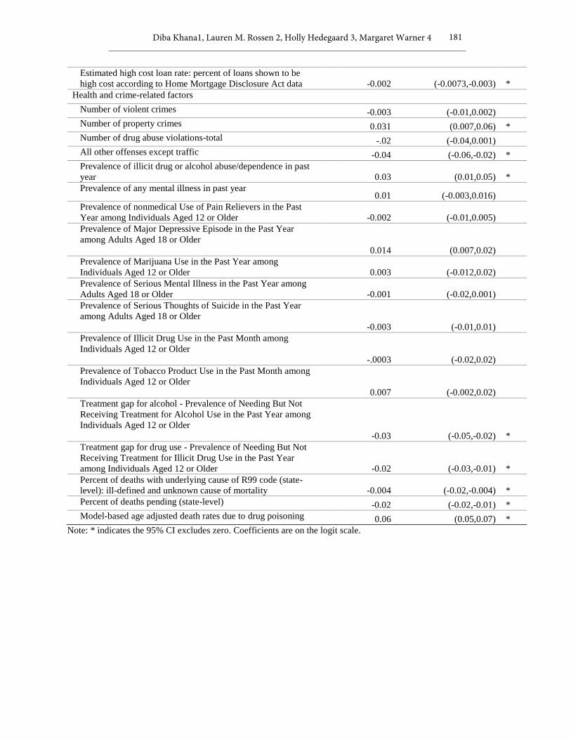
3.5 Covariates

The inclusion of covariates can enhance the predictive power of small area estimation models. (Rao,

J.N.K. (2003)) Several covariates were significant predictors of county-level SRs (i.e., 95% Bayesian

Credible Intervals excluded zero). Coefficients and 95% Bayesian credible intervals for covariates and

a list of significant as well as non-significant variables included in the full model are shown in the

supplemental online information in Table s2. Covariates were included in this study to enhance the

small area predictions. Thus, the coefficients should be interpreted with caution, as they represent

ecological relationships and are not suggestive of causal pathways or individual-level risk factors.

Broadly, covariates significantly associated with SRs included: demographic characteristics (e.g.,

household size, racial and ethnic distribution, urbanization level, divorce rates), socioeconomic factors

(e.g., median home value, median gross rent, household crowding, median per capita income, %

persons with college education, unemployment rate, high-cost loan rate), and health-related

characteristics (e.g., % abusing or dependent on illicit drugs or alcohol in the previous year, treatment

gap for alcohol and drug use, prevalence of major depressive episode, and county-level model-based

estimates of age-adjusted death rates due to drug poisoning). This is consistent with prior analyses

reporting county-level (i.e., ecological) associations between socioeconomic, demographic and/or

health-related factors and suicide rates. (Brenner, B. et al. (2011), Crosby, A.E. et al. (2011), Haws, C.

A. (2009) , Hempstead, K. (2006), Kerr, W.C. et al. (2016), Kim, N. (2011), Lester, D. (1995), Miller,

M. et al. (2006), Opoliner, A. et al. (2014), Siegel, M. and Rothman, E. F. (2016))

3.6 Spatio-temporal variation

The actual number of deaths due to suicide at the county level for the year 2015 (number of deaths

less than 20 are suppressed) are shown in Figure 3. This map precludes examination of geographic

variations in county level SRs because most of the actual county level data extracted from the NVSS

files are suppressed. The majority of counties across the U.S. report fewer than 20 suicide deaths in

any given year, the criterion for suppression of death rates due to concerns about statistical reliability

by the Division of Vital Statistics at the National Center for Health Statistics. (Kochanek, K.D. et al.

(2016), page 118). The maps obtained by mapping stable posterior predictions from the best fitting

Bayesian spatio-temporal for the county-level SRs for the years 2005 (Figure 4 (top)) and 2015 (Figure

4 (bottom)) enable examination of the geographic patterns and broad scale trend in spatio-temporal

variability for the years 2005 and 2015 for all of the counties. The uncertainty associated with the

estimated county level SRs for the years 2005 and 2015 is very small as shown in Figure S5 (2005 (top)

and 2015 (bottom)) in the Appendix. A comparison of the aggregated state level SRs obtained by

aggregating county level SRs via MCMC simulations in the software Winbugs with the same modeling

assumptions as in Section 3.2 and vague prior distributions specifications, showed that the predictions

are almost the same (Figure S6 in the Appendix), further solidifying our belief in the INLA based

predictions. However, the MCMC programs took 8 weeks to converge in the software Winbugs.

In 2005 and 2015, counties with the highest model-based SRs were predominantly located across

the western US while the lowest rates were observed across southern California, western Texas, along

the Mississippi river, and in areas along the East Coast. These patterns were largely consistent over

time. Multiple studies have described state-level variation in suicide rates (SRs), with higher rates noted

in Western states lending credibility to the model based county level SRs. (Karch, L.D. et al. (2009),

Kposowa, A.J. (2013)) This further validates our belief in statistical modelling assumptions.

Additionally, the maps for the years 2005 (Figure 4 (top)) and 2015 (Figure 4 (bottom)) with robust

and reliable county level estimates highlight all counties with high and low suicides mortality which


can be used to target prevention programs and for more effective allocation of resources. Hence, the

existing Bayesian spatio-temporal techniques in R-INLA outlined in this study can be useful in

analyzing the trend and changing spatial patterns of a small area outcome such as SRs at the county

level not afforded by examination of direct state estimates, national estimates and direct county level

estimates.

The absolute differences in the model based county level SRs in the U.S. from 2005-2015 are

shown in Figure 5. The absolute differences map of the posterior predictions of the county level SRs

depicts the magnitude of change in spatio-temporal variability in county level SRs for the years 2005

and 2015. Approximately 77% (2418) counties reported an absolute difference between 1 and 5 in the

model based county level SRs for the years 2005 and 2015. The spatial patterning of the random effects

can be seen in Figure 6 accounting for the large correlated heterogeneity in areas where the SRs are

high. This supports our choice of using a spatially structured random effects model. The extra

uncorrelated variability is seen in Figure 7. Thus, the existing hierarchical Bayesian spatio-temporal

models in R-INLA can account for the differences in time and the challenges associated with examining

unreliable direct estimates for less common causes of mortality outcomes for small scale geographic

data and produce robust and reliable estimates enabling examination of spatiotemporal variations

4 Discussion

County-level direct estimates of less common mortality outcomes are often highly unstable. Many

prior studies on county-level variations in less common causes of mortality outcomes have relied on

estimates aggregated over time or larger geographic areas. However, this type of aggregation precludes

the examination of detailed temporal and spatial trends. To overcome these limitations, this study uses

hierarchical Bayesian methods to generate robust model-based estimates of yearly county-level SRs to

examine the spatio-temporal variations across a span of 11 years.

This study contributed to the existing literature by applying an existing methodology, namely

hierarchical Bayesian spatio-temporal models in R-INLA to estimate county-level SRs in order to

examine spatiotemporal variation in SRs. Although there are a variety of alternative models with

different assumptions that we did not explicitly explore, this study is the first to incorporate

spatiotemporal random effects along with time varying confounders to estimate annual county level

estimates for SRs for the years 2005-2015. There was substantial geographic variation in SRs. The

majority of the counties across the U.S. demonstrated an increase in suicide death rates over this time

period and no counties exhibited a decline. The existing Bayesian spatio-temporal modeling techniques

in R-INLA can potentially be applied to a large number of rare causes of mortality-related outcomes

from vital statistics data to examine geographic and temporal variation.

The use of R-INLA method resulted in substantially reduced computation time for this study, an

average of twenty four for the best model with a full set of covariates and six to twenty four hours for

models with no or few covariates, as opposed to weeks of time required for simulations based Markov

Chain Monte Carlo (MCMC) via WINBUGS with large spatial datasets. (Khan, D. et al. (2018),

Martins, T.G. et al. (2013), Rockett, I.R. et al. (2012), Rue, H. and Martino, S. (2009)) A variety of

models incorporating space and time random effects could be tested in R-INLA without an

overwhelming burden of computation time. INLA provides substantial flexibility with several built-in

model components and specifications to examine a variety of models such as proper CAR

(Conditionally autoregressive), ZIP (Zero Inflated Poisson) and Besag Proper without the need of

further programming expertise. Moreover, the functional form of the covariates in R-INLA can be

specified in different forms and can be other than linear as well.


The model fit was examined via DIC comparisons. Amongst the models fitted, the contribution of

different space and time components was examined by the subsequent reduction in DIC values and the

effective number of parameters to estimate. The best-fitting model captured the spatial autocorrelation

and the time dependence structure of the data and was further improved by using time varying

covariates accounting for the extra variability that was not captured by the main time and county effects.

The best fitting model was found to have the lowest DIC with small number of effective parameters to

estimate as compared to the model without time varying covariates. However, the temporal random

effect was found to be an autoregressive process of order 1 which dampens out after a certain period

of time. This suggests that future analyses might not require too long of a stretch of data in time in

order to compute stable county level SRs. The comparison of state-level directly estimated SRs and the

aggregated model-based state-level SRs for the different years showed that the majority of estimates

fell on the line of equality indicating a close correspondence between the model-based state SRs and

the direct state SRs at larger geographic scales.

The limitations of this study are as follows. Although a large number of models were implemented,

alternative models incorporating different covariates from other data sources and space and time

components might have improved the predictions. Secondly, R-INLA software can implement a variety

of traditional models that are built-in, however there are a class of models such as latent mixture models

that still need to be implemented. Moreover, the prior specifications that are not built-in in R-INLA

need to be programmed. Thirdly, this study incorporated a large number of covariates to account for

measured covariates, however suicides rates vary by gender and age groups and future studies can look

at suicide rates by these mechanisms. Lastly, there is underreporting in suicides numbers and the actual

number of suicides are always larger than the reported. Underreporting and measurement errors in

suicides cannot be understated and have been studied in the literature (Claassen, C.A. et al. (2010)).

Future studies can consider more explicit handling of the prior distributions other than the default

priors specified in R-INLA (Simpson, D. et al. (2017)). Future research exploring spatial clustering of

less common causes of mortality outcomes over time, including at sub-county levels, would provide

further understanding of how the small-scale geographic variation may be spatially patterned across

the U.S. Lastly, the R-INLA package has provided a new, flexible and substantially faster alternative

to MCMC methods.


References

[1] Area Health Resource Files (2015). US Department of Health and Human Services, Health

Resources and Services Administration, Bureau of Health Workforce. Area Health Resources

Files (Rockville, MD).

[2] Barker, L. E., Thompson, T. J., Kirtland, K. A., Boyle, J. P., Geiss, L. S., McCauley, M. M. and

Albright, A. L. (2013) Bayesian small area estimates of diabetes incidence by United States

county, 2009. J. Data Sci., 11, 249–267.

[3] Besag, J. and Kooperberg, C. (1995). On conditional and intrinsic autoregressions. Biometrika 82,

733–746.

[4] Besag, J., York, J. and Mollie A. (1991). Bayesian image restoration, with two applications in

spatial statistics. Annals of the Institute of Statistical Mathematics 43:1-20.

[5] Betz, M. E., Valley, M. A., and Lowenstein, S. R., Hedegaard, H., Thomas, D., Stallones, L., and

Honigman, B. (2011). Elevated suicide rates at high altitude: sociodemographic and health issues

may be to blame. Suicide Life Threat Behav 41:562-573.

[6] Bivand, R. S., Rubio-Gomez, V., Rue, H. (2015). Spatial Data Analysis with R-INLA with Some

Extensions. Journal of Statistical Software 63.

[7] Bivand, R. Creating Neighbours. (2017). The Comprehensive R Archive Network. Vol 2017 2017.

[8] B ohning, D., Dietz, E. and Schlattmann, P. (2000). Space-time mixture modelling of public health

data. Statist.Med. 19, 2333–2344.

[9] Breiding, M. J. and Wiersema, B. (2006). Variability of undetermined manner of death

classification in the US. Inj Prev. 12 Suppl 2:ii49-ii54.

[10] Brenner, B., Cheng, D., Clark, S., Camargo Jr., C. A. (2011). Positive association between altitude

and suicide in 2584 U.S. counties. High Alt Med Biol. 12:31-35.

[11] Centers for Disease Control and Prevention, National Center for Health Statistics. (2016). Multiple

Cause of Death 1999-2015 on CDC WONDER Online Database, released December, 2016. Data

are from the Multiple Cause of Death Files, 1999-2015, as compiled from data provided by the

57 vital statistics jurisdictions through the Vital Statistics Cooperative Program.

http://wonder.cdc.gov/ucd-icd10.html

[12] Chen, C., Wakefield, J., Lumley, T. (2014). The use of sampling weights in Bayesian hierarchical

models for small area estimation. Spatial and Spatiotemporal Epidemiology 11: 33–43.

[13] Cheng, D. (2010). Higher suicide death rate in rocky mountain states and a correlation to altitude.

Wilderness Environ Med. 21:177-178.

[14]Claassen, C.A., Yip, S. P., Corcoran, P., Bossarte, R.M., Lawrence, B.A., and Currier, G.W. (2010).

National suicide rates a century after Durkhleim: Do we know enough to estimate error? Suicide

and Life-Threatening Behavior. 40 (3) June 2010.


[15] Crosby, A. E., Han, B., Ortega, L. A., Parks, S. E., and Gfroerer, J. (2011). Suicidal thoughts and

behaviors among adults aged >/=18 years--United States, 2008-2009. MMWR Surveill Summ.

60:1-22.

[16] Curtin, S.C., Warner, M., Hedegaard, H. (2016). Increase in Suicide in the United States, 1999-

2014. NCHS Data Brief. 1-8.

[17] Fong, Y., Rue, H., Wakefield, J. (2010). Bayesian inference for generalized linear mixed models.

Biostatistics. 11:397–412. [PubMed: 19966070]

[18] Haws, C. A., Gray, D. D., Yurgelun-Todd, D. A., Moskos, M., Meyer, L. J., Renshaw, P. F. (2009).

The possible effect of altitude on regional variation in suicide rates. Med Hypotheses 73:587-590.

[19] Hempstead, K. (2006). The geography of self-injury: spatial patterns in attempted and completed

suicide. Soc Sci Med.;62:3186-3196.

[20] Hempstead, K. A. (2015). Phillips. J. A. Rising suicide among adults aged 40-64 years: the role of

job and financial circumstances. Am J Prev Med. 2015;48:491-500.

[21] Houle, J. N. and Light, M. T. (2014). The home foreclosure crisis and rising suicide rates, 2005 to

2010. Am J Public Health 104:1073-1079.

[22] Karch, D. L., Dahlberg, L. L., Patel, N., Davis, T. W., Logan, J. E., Hill, H. A. (2009). Surveillance

for violent deaths–National Violent Death Reporting System, 16 states, 2006. MMWR

Surveillance Summaries, 58, 1–44.

[23] Kerr, W. C., Kaplan, M. S., Huguet, N., Caetano, R., Giesbrecht, N., McFarland, B. H. (2016).

Economic Recession, Alcohol, and Suicide Rates: Comparative Effects of Poverty, Foreclosure,

and Job Loss. Am J Prev Med.

[24] Khan, D., Rossen, L., Hamilton, B., Dienes, E., Wei, R., He, Y. (2018). Spatiotemporal trends in

teen birth Rates in the U.S., 2003-2012. Journal of the Royal Statistical Society, Series A (To

appear 2018). Available online: http://onlinelibrary.wiley.com/doi/10.1111/rssa.12266/epdf

[25] Kim, N., Mickelson, J. B., Brenner, B. E., Haws, C. A., Yurgelun-Todd, D. A., Renshaw, P. F.

(2011). Altitude, gun ownership, rural areas, and suicide. Am J Psychiatry. 168:49-54.

[26] Knorr-Held, L. and Besag, J. (1998) Modelling risk from a disease in time and space. Statist. Med.,

17, 2045–2060.

[27]Knorr-Held L, Rasser, G. (2000). Bayesian detection of clusters and discontinuities in disease maps.

Biometrics 56:13-21.

[28] Kochanek, K. D., Murphy, S. L., Xu, J. Q., Tejada-Vera, B. (2016). Deaths: Final data for 2014.

National vital statistics reports; vol 65:1-122, no 4. Hyattsville, MD: National Center for Health

Statistics.

[29] Kposowa, A. J. (2013). Association of suicide rates, gun ownership, conservatism and individual

suicide risk. Soc Psychiatry Psychiatr Epidemiol vol 48: 1467. doi:10.1007/s00127-013-0664-4


[30] Lagazio, C., Dreassi, E. and Biggeri, A. (2001) A hierarchical Bayesian model for space-time

variation of disease risk. Statist. Modllng, 1, 17–29.

[31] Lawson, A. (2013). Bayesian Disease Mapping: Hierarchical Modeling in Spatial Epidemiology.

Boca Raton, FL: Chapman & Hall/CRC Press.

[32] Lawson, A. (2015). Bayesian Disease Mapping: Hierarchical Modeling in Spatial Epidemiology.

Workshop notes (unpublished).

[33] Lester, D. (1995). Explaining regional differences in suicide rates. Soc Sci Med. 40:719-721.

[34] Lunn, D., Jackson, C., Best, N., Thomas, A. and Spiegelhalter, D. (2013). The BUGSBook: a

Practical Introduction to Bayesian Analysis. Boca Raton: Chapman and Hall–CRC.

[35] Lee, D. (2013). CARBayes: an R package for Bayesian spatial modeling with conditional

autoregressive priors. J. Statist. Softwr., 55, no. 13, 1–24.

[36] Martins, T. G., Simpson, D., Lindgren, F, H. R. (2013). Bayesian computing with INLA: New

features. Journal of Computational Statistics and Data Analysis 67:68-83.

[37] Middleton, N., Sterne, J. A. and Gunnell, D. J. (2008). An atlas of suicide mortality: England and

Wales, 1988-1994. Health Place 14:492-506.

[38] Miller, M., Azrael, D. and Hemenway, D. (2002). Household firearm ownership and suicide rates

in the United States. Epidemiology 13:517-524.

[39] Miller, M., Azrael, D., Hepburn, L., Hemenway, D., Lippmann, S. J. (2006). The association

between changes in household firearm ownership and rates of suicide in the United States, 1981-

2002. Inj Prev. 12:178-182.

[40] National Center for Health Statistics Centers for Disease Control and Prevention. (2015). NCHS

Urban-Rural Classification Scheme for Counties.

[41] National Center for Health Statistics. (2011). Estimates of the April 1, 2010 resident population of

the United States, by county, single-year of age (0, 1, 2, …, 85 years and over), bridged race,

Hispanic origin, and sex. Prepared under a collaborative arrangement with the U.S. Census

Bureau.

[42] National Center for Health Statistics. (2016a). Vintage 2015 postcensal estimates of the resident

population of the United States (April 1, 2010, July 1, 2010-July 1, 2015), by year, county, single-

year of age (0, 1, 2, .., 85 years and over), bridged race, Hispanic origin, and sex. Prepared under

a collaborative arrangement with the U.S. Census Bureau.

[43] National Center for Health Statistics. (2016b). Bridged-race intercensal estimates of the resident

population of the United States for July 1, 2000-July 1, 2009, by year, county, single-year of age

(0, 1, 2, .., 85 years and over), bridged race, Hispanic origin, and sex. Prepared under a

collaborative arrangement with the U.S. Census Bureau.

[44] National Center for Health Statistics (2016c). County Geography Changes: 1990-2015:1-7.

https://www.cdc.gov/nchs/nvss/bridged_race/county_geography-_changes2015.pdf


[45] National Survey on Drug Use and Health. (2016). Subtance Abuse and Mental Health Services

Administration (SAMHSA). Rockville, MD. Substate Estimates.

[46] Ntzoufras, I. (2009). Bayesian Modeling using Winbugs. Hoboken: Wiley.

[47] Opoliner, A., Azrael, D., Barber, C., Fitzmaurice, G., Miller, M. (2014). Explaining geographic

patterns of suicide in the US: the role of firearms and antidepressants. Inj Epidemiol. 1:6.

[48] Paul, M., Riebler, A., Bachmann, L., Rue, H., Held, L. (2010). Bayesian bivariate meta-analysis

of diagnostic test studies using integrated nested laplace approximations. Statistics in Medicine.

vol 29:1325–1339. [PubMed: 20101670]

[49] Plummer, M. (2003). JAGS: A Program for Analysis of Bayesian Graphical Models Using Gibbs

Sampling, Proceedings of the 3rd International Workshop on Distributed Statistical Computing

(DSC 2003), March 20–22, Vienna, Austria. ISSN 1609-395X.

[50] Rao, J.N.K. (2003) Small area estimation. Hoboken, NJ: Wiley.

[51] Rezaeian, M., Dunn, G., St. Leger, S., Appleby, L. (2007). Do hot spots of deprivation predict the

rates of suicide within London boroughs? Health Place. 13:886-893.

[52] Riebler, A, Held, L., Rue, H. (2012). Estimation and extrapolation of time trends in registry data –

borrowing strength from related populations. Annals of Applied Statistics. 6:304–333.

[53] Rockett, I. R., Hobbs, G. R., Wu, D., Jia, H., Notte, K. B., Smith, G.S., Putnam, S. L, Caine, E. D.

(2015). Variable Classification of Drug-Intoxication Suicides across US States: A Partial Artifact

of Forensics? PLoS One. 2015;10:e0135296.

[54] Rue, H, Martino, S. (2009). INLA: Functions which allow to perform a full Bayesian analysis of

structured additive models using Integrated Nested Laplace Approximation. R package, version

0.0.

[55] Rue, H., Martino, S., Chopin, N. (2009). Approximate Bayesian inference for latent Gaussian

models by using integrated nested Laplace approximations. Journal of the Royal Statistical

Society Series B -Statistical Methodology 71:319-392.

[56] Schaible, W. L. (1996) Indirect Estimators in U.S. Federal Programs (Lecture Notes in Statistics.

Springer, New York.

[57] Schrodle, B., Held, L., Riebler, A., Danuser, J. (2011). Using INLA for the evaluation of veterinary

surveillance data from Switzerland: A case study. Journal of the Royal Statistical Society, Series

C. 60:261–279.

[58]Siegel, M., Rothman, E. F. (2016). Firearm ownership and suicide rates among US men and women,

1981-2013. Am J Public Health. 106:1316-1322.

[59] Simpson, D., Rue, H., Riebler A., Martins, T.G., Sorbye, S.H. (2017). Penalising Model

Component Complexity: A Principled, Practical Approach to Constructing Priors. Statist Sci.

Volume 32, Number 1 (2017), 1-28.


[60] Spiegelhalter, D. J., Best, N. G., Carlin, B. P., and van der Linde, A. (2002). Bayesian measures of

model complexity and fit (with discussion). Journal of the Royal Statistical Society (Series B)

64:5830639.

[61] Stan Development Team. (2016). RStan: the R interface to Stan. R package version 2.14.1.

http://mc-stan.org

[62] Sterrantino, A., F., Ventrucci, M, and Rue, Haavard (2017). A note on intrinsic Conditional

Autoregressive models for disconnected graphs. arXiv:1705.04854v1.

[63] Uniform Crime Reporting Program Data. (2014). United States Department of Justice. Federal

Bureau of Investigation. Uniform Crime Reporting Program Data: County-Level Detailed Arrest

and Offense Data. Ann Arbor, MI: Inter-university Consortium for Political and Social Research

2014.

[64] U.S. Department of Housing and Urban Development. (2017). HUD Provided Local Level Data.

[65] Wall, M. M. (2004). A close look at the spatial structure implied by the CAR and SAR models. J.

Statist. PlanngInf., 121, 311–324.

[66] Xia, H., Carlin, B. P. and Waller, L. A. (1997) Hierarchical models for mapping Ohio lung cancer

rates. Environmetrics, 8, 107–120.

Tables

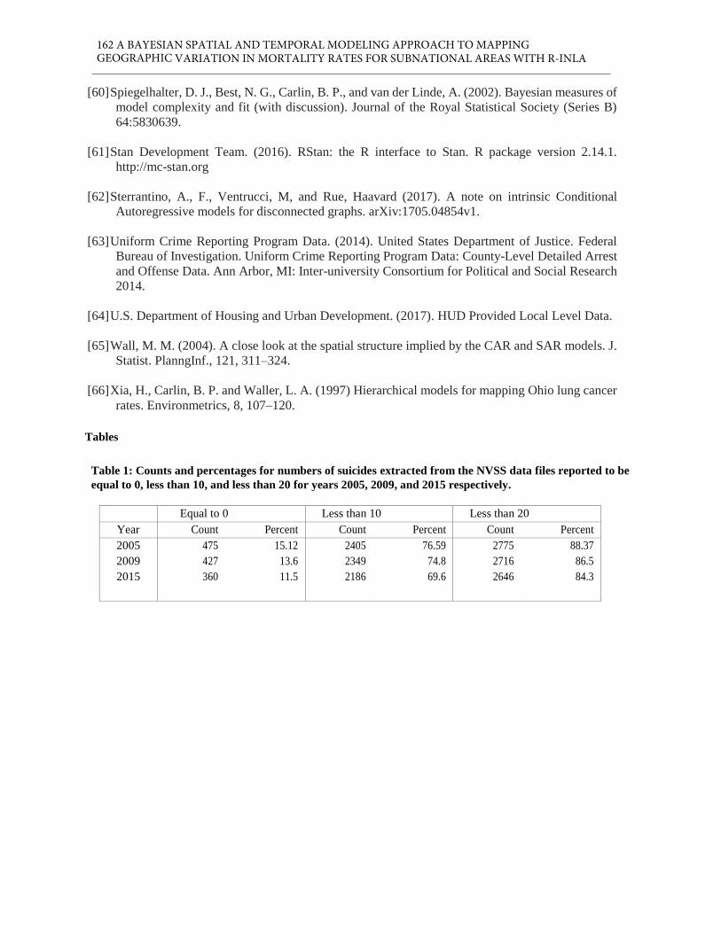
Table 1: Counts and percentages for numbers of suicides extracted from the NVSS data files reported to be

equal to 0, less than 10, and less than 20 for years 2005, 2009, and 2015 respectively.

Equal to 0 Less than 10 Less than 20

Year Count Percent Count Percent Count Percent

2005 475 15.12 2405 76.59 2775 88.37

2009 427 13.6 2349 74.8 2716 86.5

2015 360 11.5 2186 69.6 2646 84.3


http://mc-stan.org/

https://arxiv.org/abs/1705.04854v1

Table 2. Alternative Model Specification and Fit Statistics

Terms: 𝛼0 represents the intercept or grand mean; 𝑢𝑖 is a spatial random effect; 𝑣𝑖 is a non-spatial random effect;

𝜑1𝑡 and 𝜑2𝑡 are the temporal random effects, 𝜓𝑖𝑡 is the space-time interaction term, which is independently and

identically distributed, accounting for any residual spatiotemporal variation; and 𝑿𝒊𝒕′𝜷 represent the matrix of time-

varying covariates and the corresponding coefficients.

Table 3. Model hyperparameters: posterior mean, posterior standard deviation, 95% Bayesian credible

intervals and posterior mode for the estimated marginals of the precisions of the prior variances of non-

spatial effects, 𝜏𝑣 , spatial effects, 𝜏𝑢 , correlated time effect, 𝜏𝜑1 and iid space time interaction effect, 𝜏𝜓.

Precisions Posterior mean Posterior

standard

deviation

0.025 quantile 0.975 quantile Posterior mode

𝜏𝑣 22380.75 2009.316 2523.08 75191.57 7201.39

𝜏𝑢 21.27 1.439 18.85 24.46 20.68

𝜏𝜑1 5935.05 3180.924 2062.85 14120.89 4046.36

𝜏𝜓 461.13 78.305 335.38 641.15 428.46

Model Components DIC n.eff

1.Simple random effects, 𝑣𝑖 𝛼0 + 𝑣𝑖 150371.4 2316

2.Spatial 𝑢𝑖 and non-Spatial 𝑣𝑖 , random effects 𝛼0 + 𝑢𝑖 + 𝑣𝑖 149966.2 2316

Random time effects

3. Correlated time effects, 𝜑1𝑡 𝛼0 + 𝑢𝑖 + 𝑣𝑖 + 𝜑1𝑡 148008.6 1884

4. Uncorrelated time effects, 𝜑2𝑡

Full Model

𝛼0 + 𝑢𝑖 + 𝑣𝑖 + 𝜑2𝑡 148010.3 1886

5. Space time interaction term, 𝜓𝑖𝑡 𝛼0 + 𝑢𝑖+𝑣𝑖 + 𝜑2𝑡+𝜓𝑖𝑡 147821.9 2766

Full Model with Covariates

6. All components and covariates 𝛼0 + 𝑢𝑖 + 𝑣𝑖 + 𝜑1𝑡+𝜓𝑖𝑡+𝑿𝒊𝒕′𝜷 147181.1 1896


FIGURES

Figure 1. Comparison of state-level direct estimates (y-axis) and model-based estimates (x-axis), by year.


Figure 2. Shrinkage of suicide rates for each state, by population size for 2015. Crude death rates are plotted at the

start of the arrows, and model-based death rates are located at the end of the arrows. Shrinkage is greater in states

with smaller populations (left side of the chart) and more extreme suicide rates.


Figure 3: Crude county level deaths due to suicides for the year 2015. Number of deaths less than 20 are

suppressed.


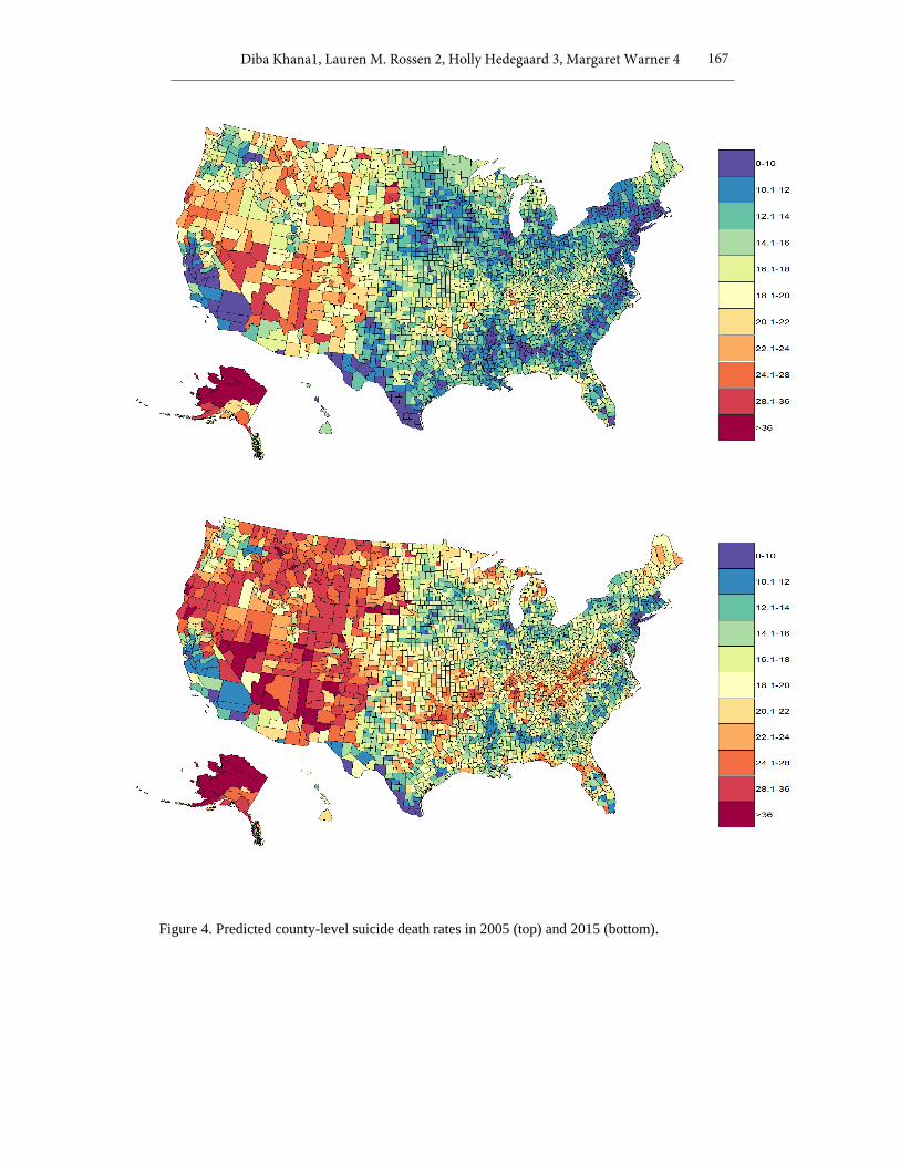
Figure 4. Predicted county-level suicide death rates in 2005 (top) and 2015 (bottom).


Figure 5. Absolute differences in model based county level suicide rates in the U.S. from 2005-2015. (The

legend corresponds to the increase in suicide number of deaths per 100,000)


Figure 6. Spatially structured random effect representing correlated heterogeneity in suicide rates across

U.S. counties.


Figure 7. Spatially unstructured random effect representing uncorrelated heterogeneity in suicide rates

across U.S. counties.


Supplemental Online Information

Figure S1. Scatterplot of posterior estimates of suicide rates, model with no covariates vs. model with all covariates.


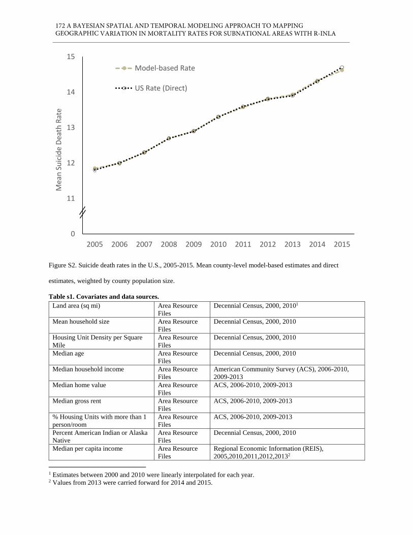
Figure S2. Suicide death rates in the U.S., 2005-2015. Mean county-level model-based estimates and direct

estimates, weighted by county population size.

Table s1. Covariates and data sources.

Land area (sq mi) Area Resource

Files

Decennial Census, 2000, 20101

Mean household size Area Resource

Files


Housing Unit Density per Square

Mile

Area Resource

Files


Median age Area Resource

Files


Median household income Area Resource

Files

American Community Survey (ACS), 2006-2010,

2009-2013

Median home value Area Resource

Files

ACS, 2006-2010, 2009-2013

Median gross rent Area Resource

Files

ACS, 2006-2010, 2009-2013

% Housing Units with more than 1

person/room

Area Resource

Files

ACS, 2006-2010, 2009-2013

Percent American Indian or Alaska

Native

Area Resource

Files


Median per capita income Area Resource

Files

Regional Economic Information (REIS),

2005,2010,2011,2012,20132

1 Estimates between 2000 and 2010 were linearly interpolated for each year. 2 Values from 2013 were carried forward for 2014 and 2015.

10

11

12

13

14

15

2005 2006 2007 2008 2009 2010 2011 2012 2013 2014 2015

Mea

n S

uic

ide

Dea

th R

ate

Model-based Rate

US Rate (Direct)


Percent Asian Area Resource

Files


Percent non-Hispanic Black Area Resource

Files


% Persons aged 25+ w/ 4+ Yrs

College

Area Resource

Files

ACS, 2006-2010, 2009-2013

Percent of females divorced Area Resource

Files

ACS, 2006-2010, 2009-2013

Percent female headed household Area Resource

Files


Percent foreign born Area Resource

Files

ACS, 2006-2010, 2009-2013

Percent Hispanic Area Resource

Files


% Persons aged 25+ w/ High

School Diploma

Area Resource

Files

ACS, 2006-2010, 2009-2013

% Persons aged 25+ w/ less than

High School Diploma

Area Resource

Files

ACS, 2006-2010, 2009-2013

Percent in owner-occupied housing Area Resource

Files


Percent below the poverty level Area Resource

Files

Census SAIPE, 2005,2006,2007,2008,2009,2010,

2011,2012,20133

Percent rural population Area Resource

Files


Percent urban population Area Resource

Files


Percent non-Hispanic White Area Resource

Files


Percent workers in

agriculture/forestry/fishing/hunting/

mine work

Area Resource

Files

ACS, 2006-2010, 2009-2013

Percent workers in construction Area Resource

Files

ACS, 2006-2010, 2009-2013

Percent workers in

Education/Healthcare/Social

Assistance

Area Resource

Files

ACS, 2006-2010, 2009-2013

Percent workers in manufacturing Area Resource

Files

ACS, 2006-2010, 2009-2013

Percent workers in Other Industries Area Resource

Files

ACS, 2006-2010, 2009-2013

Unemployment rate, 16+ Area Resource

Files

Bureau of Labor Stats (BLS),

2005,2010,2011,2012,2013,20144

Veteran population estimate Area Resource

Files

Dept of Veteran’s Affairs,

2005,2006,2007,2008,2009,2010,

2011,2012,2013,2014,2015

Number of violent crimes Uniform Crime

Reporting

Program Data:

County-Level

2005,2006,2007,2008,2009,2010,2011,2012,2013,201

45

3 Values from 2013 were carried forward for 2014 and 2015. 4 Values from 2014 were carried forward to 2015. 5 Values from 2014 were carried forward to 2015.


Detailed Arrest

and Offense Data

Number of property crimes Uniform Crime

Reporting

Program Data:

County-Level

Detailed Arrest

and Offense Data

2005,2006,2007,2008,2009,2010,2011,2012,2013,201

4

Number of drug abuse violations-

total

Uniform Crime

Reporting

Program Data:

County-Level

Detailed Arrest

and Offense Data

2005,2006,2007,2008,2009,2010,2011,2012,2013,201

4

All other offenses except traffic Uniform Crime

Reporting

Program Data:

County-Level

Detailed Arrest

and Offense Data

2005,2006,2007,2008,2009,2010,2011,2012,2013,201

4

Estimated number of foreclosure

starts divided by number of

mortgages times 100.

Housing and

Urban

Development

Small Area

Foreclosure

Rates6

2007-20087

United States Postal Service data

from June 2008 on residential

addresses vacant 90-days or longer

Housing and

Urban

Development

Small Area

Foreclosure

Rates

20087

Estimated high cost loan rate:

percent of loans shown to be high

cost according to Home Mortgage

Disclosure Act data

Housing and

Urban

Development

Small Area

Foreclosure

Rates

2004-20068

Illicit drug or alcohol

abuse/dependence in past year

National Survey

of Drug Use and

Health Substate

Estimates

2006-2008,2008-2010,2010-20129

Any mental illness in past year National Survey

of Drug Use and

Health Substate

Estimates

2006-2008,2008-2010,2010-2012

6 https://www.huduser.gov/portal/datasets/nsp_foreclosure_data.html 7Time-invariant variable.

8 Time-invariant variable. 9 Values from the 2010-2012 data were carried forward to 2015.


Nonmedical Use of Pain Relievers

in the Past Year among Individuals

Aged 12 or Older

National Survey

of Drug Use and

Health Substate

Estimates

2006-2008,2008-2010,2010-2012

Major Depressive Episode in the

Past Year among Adults Aged 18 or

Older

National Survey

of Drug Use and

Health Substate

Estimates

2006-2008,2008-2010,2010-2012

Marijuana Use in the Past Year

among Individuals Aged 12 or

Older

National Survey

of Drug Use and

Health Substate

Estimates

2006-2008,2008-2010,2010-2012

Serious Mental Illness in the Past

Year among Adults Aged 18 or

Older

National Survey

of Drug Use and

Health Substate

Estimates

2006-2008,2008-2010,2010-2012

Had Serious Thoughts of Suicide in

the Past Year among Adults Aged

18 or Older

National Survey

of Drug Use and

Health Substate

Estimates

2006-2008,2008-2010,2010-2012

Illicit Drug Use in the Past Month

among Individuals Aged 12 or

Older

National Survey

of Drug Use and

Health Substate

Estimates

2006-2008,2008-2010,2010-2012

Tobacco Product Use in the Past

Month among Individuals Aged 12

or Older

National Survey

of Drug Use and

Health Substate

Estimates

2006-2008,2008-2010,2010-2012

Treatment gap for alcohol -

Needing But Not Receiving

Treatment for Alcohol Use in the

Past Year among Individuals Aged

12 or Older

National Survey

of Drug Use and

Health Substate

Estimates

2006-2008,2008-2010,2010-2012

Treatment gap for drug use -

Needing But Not Receiving

Treatment for Illicit Drug Use in

the Past Year among Individuals

Aged 12 or Older

National Survey

of Drug Use and

Health Substate

Estimates

2006-2008,2008-2010,2010-2012

Percent of deaths with underlying

cause of R99 code (state-level): ill-defined and unknown cause of

mortality

Mortality Data 2005,2006,2007,2008,2009,2010

2011,2012,2013,2014,2015

Percent of deaths pending (state-

level)

Mortality Data 2005,2006,2007,2008,2009,2010

2011,2012,2013,2014,2015

Model-based age adjusted death

rates due to drug poisoning

Model-Based

Drug Poisoning

Estimates

2005,2006,2007,2008,2009,2010

2011,2012,2013,201410

10 Values for 2014 were carried forward to 2015.


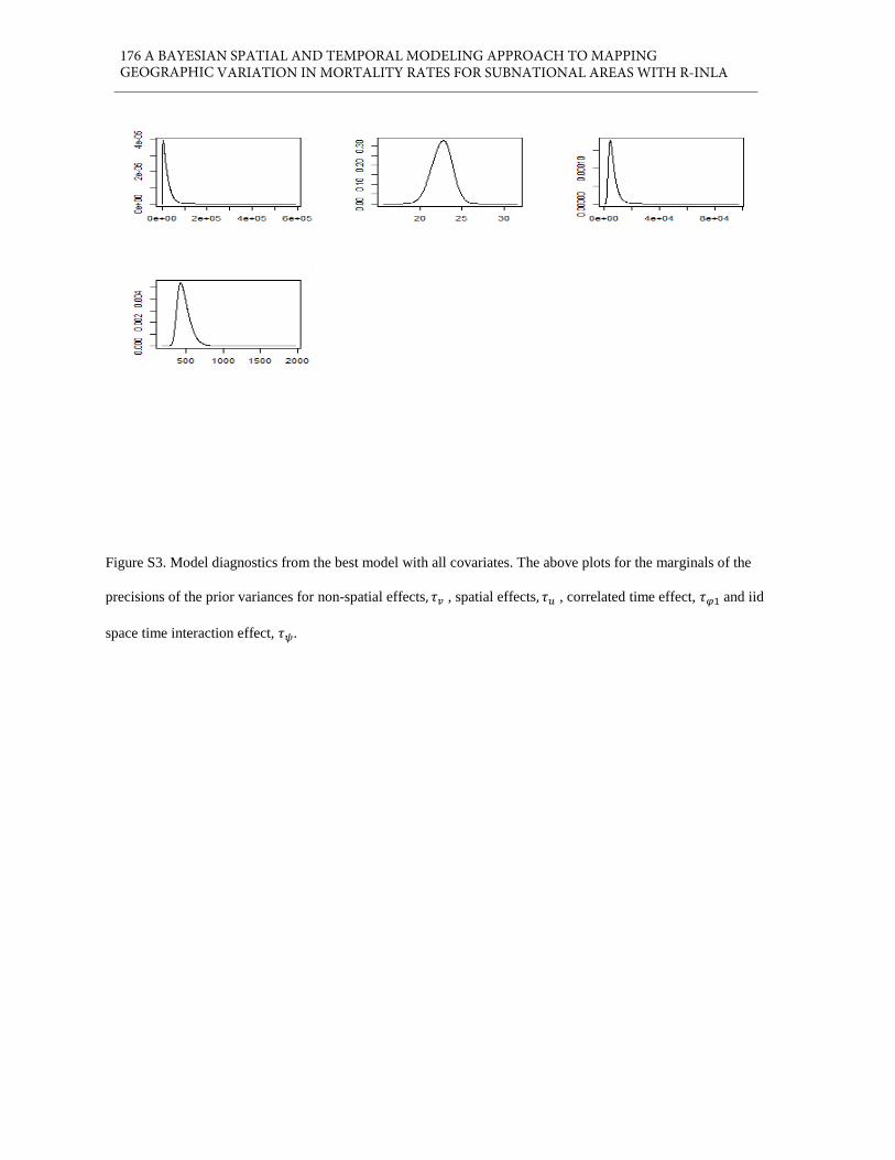
Figure S3. Model diagnostics from the best model with all covariates. The above plots for the marginals of the

precisions of the prior variances for non-spatial effects, 𝜏𝑣 , spatial effects, 𝜏𝑢 , correlated time effect, 𝜏𝜑1 and iid

space time interaction effect, 𝜏𝜓.


Figure S4. Comparison of the estimated county level SRs (top) and the associated posterior standard deviations

(bottom) obtained from the best model with all covariates using the Delaunay triangulation and sphere of influence

spatial weighting schemes.


Figure S5. Uncertainty in the county level SRs for the year 2005 (top) and 2015 (bottom) from the best model with

all covariates.


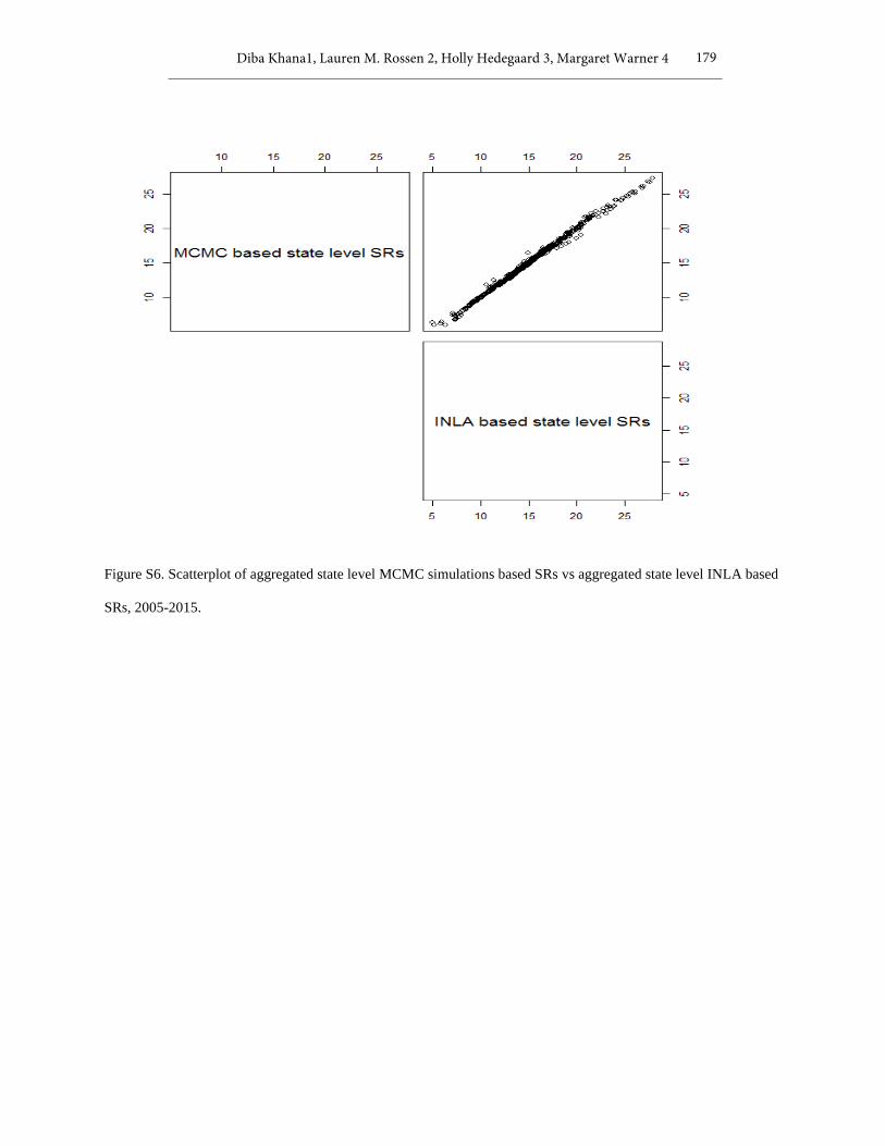
Figure S6. Scatterplot of aggregated state level MCMC simulations based SRs vs aggregated state level INLA based

SRs, 2005-2015.


Table s2. Parameter estimates and 95% credible intervals from the best fitting model

Covariate 𝛽 95% Bayesian Credible Interval

Intercept -8.76 (-8.76,-8.75) *

Demographic factors

Land area (sq mi) 0.01 (-0.002,0.02)

Mean household size -0.08 (-0.10,-0.06) *

Housing Unit Density per Square Mile -0.002 (-0.01,0.003)

Median age 0.02 (-0.0002,0.03)

Percent American Indian or Alaska Native -0.004 (-0.02,0.015)

Percent Asian -0.02 (-0.04,-0.01) *

Percent non-Hispanic Black 0.05 (0.03,0.06) *

Percent foreign born 0.04 (0.02,0.05) *

Percent Hispanic 0.04 (0.01,0.07) *

Percent non-Hispanic White 0.02 (0.01,0.03) *

Percent rural population -0.02 (-0.03,-0.005) *

Percent urban population -0.17 (-0.22,-0.12) *

Veteran population estimate -0.06 (-0.08,-0.04) *

Percent of females divorced 0.04 (0.030,0.05) *

Socioeconomic and housing-related factors

Median household income 0.06 (0.04,0.1) *

Median home value -0.02 (-0.04,-0.0003) *

Median gross rent -0.07 (-0.1,-0.04) *

% Housing Units with more than 1 person/room -15.2 (-49.36,17.4)

Median per capita income -15.2 (-49.38,17.38)

% Persons aged 25+ w/ High School Diploma 0.02 (0.001,0.04) *

% Persons aged 25+ w/ less than High School Diploma -0.01 (-0.03,0.002)

% Persons aged 25+ w/ 4+ Yrs College 0.0004 (-0.006,0.007)

Percent in owner-occupied housing -0.04 (-0.05,-0.02) *

Percent below the poverty level -0.046 (-0.09,0.002)

Percent female headed household -0.16 (-0.66,0.34)

Percent workers in agriculture/forestry/fishing/hunting/

mine work -0.03 (-0.2,0.13)

Percent workers in construction -0.1 (-0.41,0.21)

Percent workers in Education/Healthcare/Social Assistance -0.15 (-0.64,0.33)

Percent workers in manufacturing -0.15 (-0.67,0.37)

Percent workers in Other Industries 0.008 (-3.9E-05,0.017)

Unemployment rate, 16+ 0.02 (0.005,0.03) *

Estimated number of foreclosure starts divided by number of

mortgages times 100. 0.001 (-0.007,0.009)

United States Postal Service data from June 2008 on residential

addresses vacant 90-days or longer 0.01 (8.93E-05,0.016)


Estimated high cost loan rate: percent of loans shown to be

high cost according to Home Mortgage Disclosure Act data -0.002 (-0.0073,-0.003) *

Health and crime-related factors

Number of violent crimes -0.003 (-0.01,0.002)

Number of property crimes 0.031 (0.007,0.06) *

Number of drug abuse violations-total -.02 (-0.04,0.001)

All other offenses except traffic -0.04 (-0.06,-0.02) *

Prevalence of illicit drug or alcohol abuse/dependence in past

year 0.03 (0.01,0.05) *

Prevalence of any mental illness in past year 0.01 (-0.003,0.016)

Prevalence of nonmedical Use of Pain Relievers in the Past

Year among Individuals Aged 12 or Older -0.002 (-0.01,0.005)

Prevalence of Major Depressive Episode in the Past Year

among Adults Aged 18 or Older

0.014 (0.007,0.02)

Prevalence of Marijuana Use in the Past Year among

Individuals Aged 12 or Older 0.003 (-0.012,0.02)

Prevalence of Serious Mental Illness in the Past Year among

Adults Aged 18 or Older -0.001 (-0.02,0.001)

Prevalence of Serious Thoughts of Suicide in the Past Year

among Adults Aged 18 or Older

-0.003 (-0.01,0.01)

Prevalence of Illicit Drug Use in the Past Month among

Individuals Aged 12 or Older

-.0003 (-0.02,0.02)

Prevalence of Tobacco Product Use in the Past Month among


0.007 (-0.002,0.02)

Treatment gap for alcohol - Prevalence of Needing But Not

Receiving Treatment for Alcohol Use in the Past Year among


-0.03 (-0.05,-0.02) *

Treatment gap for drug use - Prevalence of Needing But Not

Receiving Treatment for Illicit Drug Use in the Past Year

among Individuals Aged 12 or Older -0.02 (-0.03,-0.01) *

Percent of deaths with underlying cause of R99 code (state-

level): ill-defined and unknown cause of mortality -0.004 (-0.02,-0.004) *

Percent of deaths pending (state-level) -0.02 (-0.02,-0.01) *

Model-based age adjusted death rates due to drug poisoning 0.06 (0.05,0.07) *

Note: * indicates the 95% CI excludes zero. Coefficients are on the logit scale.


a bayesian spatial and temporal modeling … an examination of spatio-temporal variation in less...

Documents