a behaviour based framework for the control of...
TRANSCRIPT

A Behaviour Based Framework for the
Control of Autonomous Mobile Robots
Final Year Project
Tom Walker
Supervisors: A/Prof. Thomas Braunl
A/Prof. Gary Bundell
Centre for Intelligent Information Processing Systems
School of Electrical, Electronic and Computer Engineering

ii

Tom Walker
8 Baslow Court
Carine, WA 6020
27th October 2006
The Dean
Faculty of Engineering Computing and Mathematics
The University of Western Australia
35 Stirling Highway
Crawley, WA 6009
Dear Sir,
It is with great pleasure that I submit to you this dissertation entitled “A Behaviour
Based Framework for the Control of Autonomous Mobile Robots” in partial fulfil-
ment of the requirement of the award of Bachelor of Engineering with Honours.
Yours Sincerely
Tom Walker
iii

iv

Abstract
Traditional robot control involves following a structure of perception, planning and
then action. In the perception and planning phases a world model is built up and
subsequently used to determine action. Behaviour based robotics departs from this
organisation by removing the world model and employing a structure where the
robot is controlled through a combination of parallel behavioural modules.
This project involved the design and implementation of a software framework for the
development of behaviour based applications for use with Eyesim. Basic behaviours
and a simple controller were developed to demonstrate the framework. Adaptive ca-
pabilities were implemented to extend the system and allow the robot to successfully
react to changes in the environment.
The adaptive capabilities allow for improved navigation through environments of
varying densities. The main adaptive controller was built around the Q-Learning
algorithm. This controller was trained using carefully chosen training environments
in order to optimise its performance. Q-Learning has been demonstrated to provide
a marked improvement in performance.
v

vi

Acknowledgements
I’d like to thank Thomas Braunl for providing me with the opportunity of doing
this project. It has been rewarding and intellectually stimulating experience.
Thanks to Gary Bundell for providing me with additional feedback and guidance
whilst Thomas was in Germany.
I’d also like to thank Bernard, Dave, Grace, Lixin and everyone else in the robotics
lab for their help and for helping me keep my sanity. Also, cheers to Ben, Jason,
Trev and everyone else who was generally around uni.
Finally I’d like to thank my family for proofreading my thesis and for putting up
with my coming home at absurd hours of the night. For the record, it was not a low
flying cloud.
vii

viii
Contents
Letter to the Dean iii
Abstract v
Acknowledgements vii
1 Introduction 1
1.1 Project Aims . . . . . . . . . . . . . . . . . . . . . . . . . . . . . . . 3
1.2 Dissertation Outline . . . . . . . . . . . . . . . . . . . . . . . . . . . 4
2 Background 5
2.1 Behaviour based robotics . . . . . . . . . . . . . . . . . . . . . . . . . 5
2.2 Reinforcement learning . . . . . . . . . . . . . . . . . . . . . . . . . . 6
2.2.1 Q-learning . . . . . . . . . . . . . . . . . . . . . . . . . . . . . 7
2.3 Rule-based adaptation . . . . . . . . . . . . . . . . . . . . . . . . . . 9
3 Literature Review 11
3.1 Classification of Robot Behaviours . . . . . . . . . . . . . . . . . . . 11
3.2 Architectures . . . . . . . . . . . . . . . . . . . . . . . . . . . . . . . 13
3.2.1 Subsumption . . . . . . . . . . . . . . . . . . . . . . . . . . . 13
3.2.2 Autonomous Robot Architecture . . . . . . . . . . . . . . . . 15
3.3 Adapative Control . . . . . . . . . . . . . . . . . . . . . . . . . . . . 16
ix

CONTENTS
3.3.1 Q-Learning . . . . . . . . . . . . . . . . . . . . . . . . . . . . 17
3.3.2 Learning Momentum . . . . . . . . . . . . . . . . . . . . . . . 18
3.3.3 Case-based reasoning . . . . . . . . . . . . . . . . . . . . . . . 19
4 Framework 21
4.1 Overview . . . . . . . . . . . . . . . . . . . . . . . . . . . . . . . . . . 21
4.2 Architecture . . . . . . . . . . . . . . . . . . . . . . . . . . . . . . . . 21
4.2.1 Design . . . . . . . . . . . . . . . . . . . . . . . . . . . . . . . 22
4.2.2 Implementation . . . . . . . . . . . . . . . . . . . . . . . . . . 24
4.3 Subsumption Architecture . . . . . . . . . . . . . . . . . . . . . . . . 26
4.3.1 Implementation of Subsumption . . . . . . . . . . . . . . . . . 26
5 Controller 29
5.1 Q-learning . . . . . . . . . . . . . . . . . . . . . . . . . . . . . . . . . 30
5.1.1 Task specification . . . . . . . . . . . . . . . . . . . . . . . . . 31
5.1.2 QMoveToGoal . . . . . . . . . . . . . . . . . . . . . . . . . . . 31
5.1.3 QMoveToGoal2 . . . . . . . . . . . . . . . . . . . . . . . . . . 34
5.2 Learning Momentum . . . . . . . . . . . . . . . . . . . . . . . . . . . 35
5.2.1 Rules . . . . . . . . . . . . . . . . . . . . . . . . . . . . . . . . 35
6 Navigation Task 37
6.1 Overview . . . . . . . . . . . . . . . . . . . . . . . . . . . . . . . . . . 37
6.2 Training . . . . . . . . . . . . . . . . . . . . . . . . . . . . . . . . . . 38
6.2.1 Basis . . . . . . . . . . . . . . . . . . . . . . . . . . . . . . . . 38
6.2.2 Regime . . . . . . . . . . . . . . . . . . . . . . . . . . . . . . . 39
6.2.3 Analysis . . . . . . . . . . . . . . . . . . . . . . . . . . . . . . 40
6.3 Comparison Task Environment . . . . . . . . . . . . . . . . . . . . . 44
6.4 Metrics . . . . . . . . . . . . . . . . . . . . . . . . . . . . . . . . . . . 45
x

CONTENTS
6.5 Evaluation . . . . . . . . . . . . . . . . . . . . . . . . . . . . . . . . . 45
6.5.1 Time . . . . . . . . . . . . . . . . . . . . . . . . . . . . . . . . 46
6.5.2 Path Length . . . . . . . . . . . . . . . . . . . . . . . . . . . . 47
6.5.3 Rotation . . . . . . . . . . . . . . . . . . . . . . . . . . . . . . 48
6.5.4 Collisions . . . . . . . . . . . . . . . . . . . . . . . . . . . . . 49
6.6 Paths . . . . . . . . . . . . . . . . . . . . . . . . . . . . . . . . . . . . 49
6.6.1 Cluttered environments . . . . . . . . . . . . . . . . . . . . . . 49
6.6.2 Dead-end environments . . . . . . . . . . . . . . . . . . . . . . 52
6.7 Evolution Analysis . . . . . . . . . . . . . . . . . . . . . . . . . . . . 54
7 Conclusion 57
7.1 Behaviour based frameworks . . . . . . . . . . . . . . . . . . . . . . . 57
7.2 Adaptive controllers . . . . . . . . . . . . . . . . . . . . . . . . . . . 58
7.3 Future Work . . . . . . . . . . . . . . . . . . . . . . . . . . . . . . . . 58
A Primary Framework 61
A.1 Overview . . . . . . . . . . . . . . . . . . . . . . . . . . . . . . . . . . 61
A.2 Creating behaviour . . . . . . . . . . . . . . . . . . . . . . . . . . . . 61
A.2.1 Primitive types . . . . . . . . . . . . . . . . . . . . . . . . . . 62
A.2.2 Operators . . . . . . . . . . . . . . . . . . . . . . . . . . . . . 63
A.2.3 Other . . . . . . . . . . . . . . . . . . . . . . . . . . . . . . . 64
A.3 Implemented Schemas . . . . . . . . . . . . . . . . . . . . . . . . . . 64
A.3.1 General Purpose . . . . . . . . . . . . . . . . . . . . . . . . . 64
A.3.2 EyeBot Specific . . . . . . . . . . . . . . . . . . . . . . . . . . 65
A.4 Controller Hierarchy . . . . . . . . . . . . . . . . . . . . . . . . . . . 66
A.4.1 SimpleEyebotController . . . . . . . . . . . . . . . . . . . . . 66
A.4.2 AdapativeEyebotController . . . . . . . . . . . . . . . . . . . 67
A.4.3 QLearningEyebotController . . . . . . . . . . . . . . . . . . . 67
xi

CONTENTS
A.4.4 LearningMomentumController . . . . . . . . . . . . . . . . . . 67
A.5 Sample Program: Ball-finding example . . . . . . . . . . . . . . . . . 67
B Subsumption Framework 69
B.1 Appendix for the Subsumption Framework . . . . . . . . . . . . . . . 69
B.2 Creating behaviour . . . . . . . . . . . . . . . . . . . . . . . . . . . . 69
B.2.1 Buffers . . . . . . . . . . . . . . . . . . . . . . . . . . . . . . . 69
B.2.2 Supressors . . . . . . . . . . . . . . . . . . . . . . . . . . . . . 70
B.2.3 Inhibitors . . . . . . . . . . . . . . . . . . . . . . . . . . . . . 71
B.3 Behavioural Modules . . . . . . . . . . . . . . . . . . . . . . . . . . . 72
B.3.1 General purpose . . . . . . . . . . . . . . . . . . . . . . . . . . 72
B.3.2 Eyebot Specific . . . . . . . . . . . . . . . . . . . . . . . . . . 73
B.4 Implemented Control System . . . . . . . . . . . . . . . . . . . . . . 73
C Image Processing 75
C.1 Colour space conversion . . . . . . . . . . . . . . . . . . . . . . . . . 75
C.2 Histogram Analysis . . . . . . . . . . . . . . . . . . . . . . . . . . . . 76
C.3 Determining the field of view . . . . . . . . . . . . . . . . . . . . . . 76
C.4 Retrieving object coordinates . . . . . . . . . . . . . . . . . . . . . . 77
D DVD Listing 79
References 81
xii

List of Figures
1.1 Adaptive controller concept schematic . . . . . . . . . . . . . . . . . 2
2.1 The reinforcement learning problem . . . . . . . . . . . . . . . . . . . 6
2.2 Q-Learning architecture . . . . . . . . . . . . . . . . . . . . . . . . . 8
3.1 Deliberative organisation of functional blocks . . . . . . . . . . . . . . 14
3.2 A modular and reactive organisation of control . . . . . . . . . . . . . 14
3.3 An augmented finite state machine purposed for subsumption . . . . 15
4.1 Architecture of the behaviour based framework . . . . . . . . . . . . 22
4.2 Relationship between the Controller and Motor Schemas . . . . . . . 23
4.3 Simplified class diagram showing relationships between selected schemas 24
4.4 Relationships between schemas and controller in the LocateBall task . 25
4.5 Execution-time display . . . . . . . . . . . . . . . . . . . . . . . . . . 26
4.6 Graphical display of perceived schema success . . . . . . . . . . . . . 26
4.7 Robot view as seen by Eyecam . . . . . . . . . . . . . . . . . . . . . . 26
5.1 Class hierarchy of the implemented adaptive controllers . . . . . . . . 30
5.2 Navigation task schemas coupled with an adaptive controller . . . . . 30
5.3 Behavioural assemblage used in the QMoveToGoal controller . . . . . . 32
6.1 Training environment used for both the QMoveToGoal and QMoveToGoal2
controllers (destination is highlighted) . . . . . . . . . . . . . . . . . . 40
xiii

LIST OF FIGURES
6.2 Graph of policy changes as training progresses for QMoveToGoal . . . 41
6.3 Graph of experienced reward as training progresses for QMoveToGoal . 41
6.4 Graph of policy changes as training progresses for QMoveToGoal2 . . . 42
6.5 Graph of experienced reward as training progresses for QMoveToGoal2 43
6.6 Lap times for the various controllers averaged for environment sets . . 46
6.7 Lap path lengths for the various controllers averaged for environment
sets . . . . . . . . . . . . . . . . . . . . . . . . . . . . . . . . . . . . . 47
6.8 Total rotation per lap for the various controllers averaged for envi-
ronment sets . . . . . . . . . . . . . . . . . . . . . . . . . . . . . . . . 48
6.9 Path traces for each controller in cluttered environment one . . . . . 50
6.10 Path traces for each controller in cluttered environment two . . . . . 51
6.11 Path traces for each controller in dead-end scenario one . . . . . . . . 52
6.12 Path traces for each controller in dead-end scenario two . . . . . . . . 53
A.1 Class hierarchy of the primitive types of the framework . . . . . . . . 62
A.2 Class hierarchy of the operator nodes provided by the framework . . . 63
A.3 Hierarchy of the general purpose motor schemas created for the frame-
work . . . . . . . . . . . . . . . . . . . . . . . . . . . . . . . . . . . . 65
A.4 Class hierarchy of the Eyebot-specific schemas . . . . . . . . . . . . . 66
A.5 Class hierarchy of the framework controllers . . . . . . . . . . . . . . 67
B.1 Class hierarchy of the framework SubsumptionBuffer classes as well
as the suppressor classes. . . . . . . . . . . . . . . . . . . . . . . . . . 70
B.2 Class hierarchy of the inhibitive classes . . . . . . . . . . . . . . . . . 71
B.3 Class hierarchy of the implemented behavioural modules . . . . . . . 72
B.4 Class hierarchy of the Eyebot-specific behavioural modules . . . . . . 73
B.5 Control system using self-preservation and task-oriented layers . . . . 74
C.1 Experiment configuration for determining field of view of the camera 77
C.2 Geometry used to calculate angle of an object . . . . . . . . . . . . . 77
xiv
List of Tables
5.1 Obstacle distance encoding scheme . . . . . . . . . . . . . . . . . . . 32
6.1 Parameters for the Q-Learning algorithm used in QMoveToGoal . . . 39
xv
xvi

Chapter 1
Introduction
Robotic control can be classified by two dominant paradigms: hierarchical and reac-
tive control. Hierarchical control is a top-down methodology which has its roots in
artificial intelligence theory. Reactive control is a reflexive technique characterised
by a tight coupling of sensing and action. Both paradigms have reasons for their
use, however reactive control comes into favour when higher level reasoning is not
desired, yet functionality is.
Behaviour-based control is a well established method of reactive control — in this
technique the system is described using a set of behaviours. The simplicity associ-
ated with such specification is inherently attractive. An easy to use framework for
the creation of behaviour based applications has, therefore, been developed.
Behaviour-based robotics is a control technique that is characterised by a tight
coupling between perception and action. This paradigm eschews symbolic represen-
tation of knowledge such as using a world model. Instead the system reacts to the
current environmental stimulus. Reaction to instantaneous stimulus can fail when
the system is unable to deal with conditions in which the desired actuator outputs
are not a simple function of sensory inputs. Such scenarios demonstrate a need for
the system to be able to not only react to its environment but adapt based on the
results of its reflex action.
Alternatively as the complexity of the system grows it can be harder to find a clear
mapping between sensory input and actuator output. In such systems it is highly
desirable for the developer to be able to specify the problem in a more general sense
and have the system optimise itself. Hence providing yet another need for adaptive
capabilities in behaviour based robots.
1

To these ends a framework for on-line adaptation has been created. The controllers
utilising this framework are described in more detail in Chapter 5. Figure 1.1 de-
scribes the adaptive framework in its general form.
Adaptive Controller
ΣMotor Schema
Motor Schema
Motor Schema
Schema weighting
Motor commandSchema parametersSensory
Processing
Sensory
inputs
Goal sequence
Figure 1.1: Adaptive controller concept schematic
2

INTRODUCTION
1.1 Project Aims
The aim of this project was the design and development of a software framework for
behaviour control of autonomous mobile robots. This framework was to facilitate
the easy development of behaviour based robotic applications. In addition to these
requirements the system was to have adaptive capabilities so it could be more robust
and respond to a changing environment. In response to these aims several software
components have been developed:
Behaviour based framework
The primary behaviour based framework to be developed for this project is in-
spired by the Autonomous Robot Architecture. This framework provides a set of
behavioural primitives to facilitate application development.
Adaptive controllers
Two adaptive control strategies for the primary framework have been implemented
and experimented with. The adaptive controllers provide a framework for adaptive
control of a mobile robot (using the primary behaviour based framework) as well as
some implementations of the adaptive controllers applied to a navigation task. The
framework used by these adaptive controllers is illustrated in Figure 1.1.
Secondary behaviour based framework
The secondary behaviour based framework was developed based on the Subsumption
architecture. The purpose of this framework is to provide an alternative to the AuRA
based framework. It is also of lower complexity than the primary framework and
hence more suited to deployment on actual robot hardware.
3
1.2. DISSERTATION OUTLINE
1.2 Dissertation Outline
Background
Chapter 2 briefly discusses the background theory behind systems and concepts
employed in this project. The theory behind behaviour based control is covered in
more detail in the literature review since some of the more important theory stems
from past work.
Literature Review
Chapter 3 is a review of the work done by others in the field of behaviour based
control of autonomous robots. A summary of the dominant behaviour based archi-
tectures is presented as well as a discussion on various adapative techniques that
have been applied to these architectures.
Framework
Details of the design and implementation of the behaviour based framework that
was developed for the control of autonomous mobile robots can be found in Chapter
4. The framework has been designed to enable the creation of behaviour based
applications for platforms running RoBIOS.
Adaptive Controllers
Several adapative controllers have been created for this project, these are described
in Chapter 5. Their design and development is detailed along with a brief discussion
of their relative generalised characteristics.
Navigation Task
Chapter 6 details the experiments using the aforementioned adaptive controllers.
Analysis of the data is performed and the relative merits of the adaptive controllers
are discussed.
4

Chapter 2
Background
2.1 Behaviour based robotics
Whilst the current behavioural robotics research was established in the 1980s the
concept is not a new one. In the 1930s Tolman [1] proposed a simple robot called the
sowbug. Tolman’s schematic sowbug performed similar behaviour to Braitenberg’s
vehicles [2]. Recent work by Endo and Arkin [3] has reimplemented Tolman’s design
over half a century later.
Since its early inception behaviour based robotics has become quite a broad field.
Brooks’ subsumption [4] and Arkin’s [5] AuRA provided a catalyst for a large body
of research with the result that behaviour based robotics is now a generic term.
Arkin [6] describes a number of characteristics common to behaviour based robots:
• Tight coupling of sensing to action. Behaviour based robots are composed of
reactive units that respond to stimuli without reference to a plan.
• Avoiding symbolic representation of knowledge. Behaviour based robotics es-
chews the need for a symbolic world model. The robot’s actions can be deter-
mined directly from the current sensor readings without using a representation
of the overall world.
• Decomposition into contextually meaningful units. Behaviours couple situa-
tion to action, they respond to certain situations with definite actions.
Behaviour based systems are typically composed of a number of concurrently exe-
cuting behavioural units. It is the combination of these behaviours that produces
5

2.2. REINFORCEMENT LEARNING
the overall system output. In some cases the system can be arranged such that
unexpected behaviour occurs, this is referred to as emergence. Emergence implies
a capability of the system to perform in a way that is greater than the sum of its
parts. Arkin [6] claims that whilst the individual components may be well described
the interactions between them, the environment, and the system as a whole, are
inherently complex and so there is always a margin of uncertainty in a behaviour
based system.
2.2 Reinforcement learning
Reinforcement learning is an adaptive technique whereby an agent learns through
its interaction with the environment (see Figure 2.1). A number of such learning
techniques exist, many of which are based on Sutton’s [7] work on temporal differ-
ences. Such techniques allow for agent learning with little or no a priori knowledge.
Learning occurs each time the agent performs an action and for each action the
agent receives a reward from the environment. This reward is used by the agent
to determine the validity of the particular action given its state upon making that
decision.
Learning Agent
World
ActionRewardSensory Input
(state)
Policy
World
ActionState
Return Predictor
Σ
z-1 γ
for best
action
Reward
TD
Error
+
+
-
Figure 2.1: The reinforcement learning problem as described by Sutton [8]
Sutton [8] identifies the two most important characteristics of reinforcement learning
as being the trial-and-error search and delayed rewards. Reinforcement learning
methods learn through trying actions and then receiving a delayed reward for these
actions. As reinforcement learning occurs through trial and error the problem must
be defined such that the agent can experience the whole sample-space. Careful
choice of reward function is also required otherwise the agent may learn undesirable
behaviour.
6

BACKGROUND
2.2.1 Q-learning
Q-learning is a reinforcement learning architecture proposed by Watkins [9]. Agents
using Q-learning learn based on the state of the environment and the reward received
for their actions. As in other reinforcement learning techniques agents are not told
what the desired outcomes are. Agents learn by performing actions and receiving
feedback about that action from the environment. The learning process is performed
through careful choice of states, actions and reward function to correctly specify the
problem. It is important to note that Q-learning applies a trial and error approach,
it does not perform any cognitive function such as utilising an internal world model.
The general form of the Q-learning algorithm is given as follows:
Initialise all Q(s, a) to 0
While(1) {Determine Current State
Most of the time choose action a that maximises Q(s, a)Else Pick random a
Execute aDetermine reward rUpdate Q(s, a)
}
The common form of the Q-learning algorithm has three parameters: the learning
rate (α), the discount factor (γ) and exploration probability (ε). All three param-
eters take values between 0.0 and 1.0. The learning rate determines how quickly
learning occurs. The speed of learning is determined by how quickly the Q-values
can change with action performed. If the α parameter is set too high the system
may not converge near the optimum point, however if α is too small learning may
not occur at all. The discount factor determines the value placed on future reward.
High values of γ mean that future rewards are favoured over immediate rewards.
For low values of γ the system is optimised for immediate reward. The exploration
probability is used to determine whether or not to choose the optimal action for
the given state. If ε is zero the state space may not be sufficiently explored and
optimisation may not occur.
When the agent performs an action it first checks to see if the action is exploratory.
Exploratory actions involve performing a random action from the set instead of
policy (the optimal action). If the agent is not exploring the Q-learning algorithm
chooses the optimal action for a given state from the table of Q-values. Q-values
represent the perceived benefit of an action, higher values correspond to greater
7

2.2. REINFORCEMENT LEARNING
benefit. The table of Q-values has an entry for every state/action pair. The optimal
action for a given state is the action with the highest Q-value in that state. Figure
2.2 describes the relationship between the world, policy and reward predictor.
Learning Agent
World
ActionRewardSensory Input
(state)
Policy
World
ActionState
Return Predictor
Σ
z-1 γ
for best
action
Reward
TD
Error
+
+
-
Figure 2.2: Q-Learning architecture (as described by Sutton [8]).
The basis of the Q-learning algorithm is an iterative formula (Equation 2.1). This
formula is re-evaluated each time an action is selected and the Q-value corresponding
to the previous state/action pair (s,a) is updated. The action generates a reward
(r) and puts the system into the new state (s′). maxa′Q(s′, a′) is a function that
chooses the Q-value corresponding to the optimal action a′ for the new state s′.
This form of Q-learning has been proven by Watkins and Dayan [10] to converge for
deterministic Markov decision processes.
Q(s, a)← Q(s, a) + α[r + γ maxa′ Q(s′, a′)−Q(s, a)] (2.1)
A non-deterministic approach to Q-learning (formula 2.2) is presented by Mitchell
in [11] based on work by Watkins and Dayan [10]. This version is guaranteed to
converge in systems where the reward and state transitions are given in a non-
deterministic fashion, so long as the transitions are based on a reasonable probability
8

BACKGROUND
distribution.
Qn(s, a)← (1− αn)Qn−1(s, a) + αn[r + maxa′ Qn−1(s′, a′)] (2.2)
where
αn =1
1 + visitsn(s, a)(2.3)
visitsn(s, a) is the number of times state s has selected action a at the current time
(n). Q values update more slowly than in the deterministic form of the algorithm
and the magnitude of the updates will decrease as n increases.
A third form of this equation was used by Martinson [12] for the task of behavioural
selection for a mobile robot. This equation is similar to the non-deterministic form of
Q-Learning since it applies a decay factor to both the learning rate and exploration
probability. The decay factor is determined by (1−d)n, where d is the rate of decay
and n is the number of iterations to date. Probability of exploration is initially
high, however as time progresses the system will focus less on exploration and more
on optimisation for the given environment. The decay factor that is introduced
perturbs the Q-Learning equation so that it resembles Equation 2.4.
Q(s, a)← Q(s, a) + (1− d)nα[r + γ maxa′ Q(s′, a′)−Q(s, a)] (2.4)
This approach to Q-Learning is perhaps more suited to deployment on an au-
tonomous agent. With such a configuration it can be set to initially explore the
environment and then optimise once exploration is complete.
2.3 Rule-based adaptation
Rule-based adaption can sometimes be employed as a simple learning technique. Un-
like reinforcement learning, which uses action/reward pairs, the system uses simpler
rule-based metrics to determine its next action. One example, discussed in section
3.3.2, updates system parameters according to a set of simple rules. Rule-based
adaptive methods occur in a large variety of implementations, most commonly set-
ting parameters or adjusting parameters based on the detected state of the system.
These methods have the advantage of being lightweight, since they do not learn and
9

2.3. RULE-BASED ADAPTATION
hence require less overhead, and robust given careful choice of rules. Such proper-
ties are beneficial for deployment on an autonomous robot since it allows for more
processing time to be spent on the robot’s behaviours rather than the controller
itself.
10

Chapter 3
Literature Review
3.1 Classification of Robot Behaviours
Behavioural robots are controlled by the combination of primitive behaviours. Be-
haviour primitives can be classified into a number of distinct types which in turn
can be combined to form the desired complex control systems. Arkin [6] describes
a number of distinct primitives from which complex behaviours can be composed.
Exploration/directional Exploration/directional behaviours involve the robot mov-
ing in a chosen direction. These may be behaviours such as ’move-forward’ or
’wander’. Wandering generally involves adding a random element (noise) to
the system and is a simple, if inelegant, method of preventing the robot from
getting stuck.
Goal-oriented appetitive Such behaviours involve the robot moving towards an at-
tractor. The attractor may be a region or an object, in either case the robot
will head towards it.
• e.g. returning to the recharging station as in the case of the Roomba ®
Aversive/protective Protective behaviours attempt to prevent collisions between the
robot and obstacles, either moving or stationary.
• e.g. avoiding edges of a doorway or obstacles in a corridor
Path following Path following behaviours include following a path of some kind.
Methods of determining the path and following it may vary. Paths can be
defined visually or by other methods such as pheromones (in the case of ants).
11

3.1. CLASSIFICATION OF ROBOT BEHAVIOURS
• e.g. following an underwater pipeline to examine it for damage
• e.g. following another robot
Postural Postural behaviours are those that facilitate balancing and stability of a
robot. These behaviours provide mappings between postural type sensors and
the actuators that control the robot pose in order to maintain stability even
in the face of environmental disturbance.
• e.g. robots such as Sir Arthur [13] would require some sort of postural
behaviour to enable standing balance (although the aim of that project
was evolution of the walking gait)
• e.g. Brooks’ Genghis [14] employed a postural behaviour to maintain
stability
Social/cooperative Social behaviours describe the interaction between mobile robots.
Often the behaviours used are those such as found in colony or pack creatures.
• e.g. flocking - moving in a formation that maintains some level of cohesion
but adapts in shape as the flock moves
• e.g. foraging - searching in a cooperative manner for some type of food
and returning it to the nest (useful in soccer type games)
• e.g. hunting - searching for and surrounding prey
Teleautonomous Teleautonomous behaviours allow a human operator to exert some
measure of influence over the autonomous robot. Teleautonomous control can
exert influence by using a single behaviour that receives external commands
or through a number of other methods such as using a planner which adjusts
behavioural weights based on human input. Arkin [15] demonstrated possible
use of teleautonomous behaviour by including the user input as an additional
motor schema.
Perceptual Perceptual behaviours control how the robot acquires and interprets
visual data.
• e.g. ocular reflexes - reaction to visual stimuli
Walking A walking behaviour controls the limbs of a legged robot and enables it to
move.
• e.g. Brooks’ first six-legged robot [14], Ghengis, had leg lifting behaviour
for gait control
12

LITERATURE REVIEW
• e.g. Kirchner’s Sir Arthur [13] had evolved leg behaviours and an overall
behaviour evolved for combined movement of the body segments
Manipulator-specific, gripper/dextrous hand These behaviours coordinate the move-
ment of a manipulator and the subsequent use of its end-effector to interact
with an object.
3.2 Architectures
There are currently two dominant behaviour based architectures that are widely
used: Subsumption [4] and the Autonomous Robot Architecture [5]. These two ar-
chitectures are discussed below. There are other architectures in existence, however
these make use of some of the properties presented by one of the two dominant
architectures.
3.2.1 Subsumption
The first widely published behaviour based architecture was Brooks’ [4] Subsumption
architecture in 1986. This architecture was motivated by a desire for simplicity.
Robots should be cheap and hence require little computational power to perform
their tasks. Subsumption proposed an alternative to the deliberative reasoning
paradigm of sense-plan-act, instead utilising a number of independent behaviours
executing concurrently.
Traditional Control
Prior to the introduction of subsumption most robot architectures used a deliberative
control method. Tasks were decomposed into functional blocks and each block would
be executed in turn. Generally the tasks would be perception, modeling, planning,
task execution and motor control. These can be a significant delay between the
robot sensing and the execution of its plan. Figure 3.1 illustrates the steps involved
from the sensing to actuation for a deliberative control strategy.
Layered Control
Subsumption proposes the division of control into multiple concurrent behavioural
modules. Each behaviour acts concurrently and independently and their outputs are
13

3.2. ARCHITECTURES
Sense
Model
Plan
Act
ActuatorsSensors
controller::EyebotController controller::QLearningController
controller::AdaptiveEyebotController
controller::SimpleLocateBallcontroller::VirtualController
Figure 3.1: Deliberative organisation of functional blocks
arbitrated over in some fashion. A concurrent layered control structure is illustrated
in Figure 3.2.
Plan changes to the world
Identify objects
Build maps
Discover new areas
Wander
Avoid collisions
Sensors Actuators
Figure 3.2: A modular and reactive organisation of control
Brooks [4] identified four key requirements of a control system for an intelligent
autonomous robot:
• Multiple goals - the robot must be able to satisfy multiple goals, some will be
more important than others depending on the situation.
• Multiple sensors - the robot will possess multiple sensors, it must be able to
handle conflicting results between the sensors
• Robustness - the robot must be able to adapt to changes in the environment
and sensor error
• Extensibility - the robot needs to be able to increase in processing power as
more sensors and capabilities are added
Subsumption departs from the deliberative control methods and proposes concur-
rent execution of tasks. Brooks’ solution to concurrent task execution is to have
behavioural modules that take some input and produce some output. Modules are
14

LITERATURE REVIEW
independent of each other and have no shared bus, clock or memory. Since one
behaviour should be dominant at a given time a higher-level behaviour may sub-
sume one of a lower level. This is done by sending either inhibiting or suppressing
signals to the lower level behaviour. In Brooks’ original paper [4] behaviours were
implemented as augmented finite state machines (AFSM) as in figure 3.3.
BEHAVIOURAL MODULE
I
S
R
Reset
Inhibitor
Supressor
Output linesInput lines
Figure 3.3: An augmented finite state machine purposed for subsumption
When constructing a robot control system the design may be extended layer by
layer. Initially, simple behaviours may be constructed and proven through testing
before more complex behaviour is introduced. Designed in this way, the introduction
of a new layer should not interfere with correct operation of the robot.
3.2.2 Autonomous Robot Architecture
The Autonomous Robot Architecture (AuRA) combines both reactive and deliber-
ative components. As stated by Arkin and Balch [16], the deliberative component
is broken down into a mission planner, spatial reasoner and plan sequencer. The
reactive component consists of the schema controller and the schemas. Perceptual
schemas interpret the sensory input and the motor schemas give outputs to control
the motors. The schema controller sums the outputs of the schemas in a way that
will best suit the given plan. A brief overview of schemas is given in Section 3.2.2.
Deliberative Planning
AuRA’s deliberative planner takes mission input from the operator and produces,
by combination of the spatial reasoner and plan sequencer, a plan compatible with
15

3.3. ADAPATIVE CONTROL
the behaviours of the robot. The plan sequencer then passes control of the robot
to the schema controller. If the controller completes the plan sequence or detects
a failure, control returns to the deliberative planner. In the event of failure the
planner attempts to solve the problem in a bottom up fashion. The plan sequencer
will first attempt to reroute the robot according to known data. If that fails the
spatial reasoner will decide on a new path that avoids the problematic area. Finally,
if a new path fails then the mission planner informs the operator of failure and may
request a new mission.
AuRA is a modular architecture and has been known to use various mission planners
depending on the implementation. This design has allowed experimental planners
and controllers which were designed for research in areas such as adaptive behaviour.
See Section 3.3 for more information on this topic.
Motor and Perceptual Schemas
AuRA’s reactive component uses schemas to control the robot. Schemas are pro-
posed by Arkin [5] as a basic unit of behaviour specification. Prior to [5] schemas
had been proposed by various authors using similar definitions. Each schema is in-
tended to perform a single behaviour for the robot. Perceptual schemas map sensor
readings to sensory inputs for the motor schemas. Motor schemas asynchronously
receive input from perceptual schemas and produce a vector output. AuRA’s schema
controller creates a normalised weighted sum of the vector outputs to generate the
resulting output.
3.3 Adapative Control
In order to make an autonomous robot truly useful it must be able to deal with a
changing environment. Some simple robots can simply react and require no knowl-
edge of the environment. When implementing a behaviour based system that is
linked to a deliberative mission planner the robot is required to have knowledge of
its surroundings or at least to be able to adapt as the mission changes. For these rea-
sons, and others, there has been a large amount of research done in the areas related
to machine learning. It is important to note that knowledge does not necessarily
mean a world model as in deliberative robotics. Knowledge can be identification of
a situation thus provoking the robot to react in a (possibly) predefined way to solve
a problem.
16

LITERATURE REVIEW
The most common method of employment of knowledge gained through machine
learning is through adjusting how the outputs of behaviour primitives are combined.
These approaches vary but many focus on the use of neural networks or stored
parameters (sometimes called ’cases’). Alternative methods utilise on-line adapation
using various reinforcement learning techniques.
There are a number of possible approaches to machine learning in behaviour based
robots. The techniques outlined below are all on-line adaptive methods.
3.3.1 Q-Learning
Q-learning is a form of reinforcement learning that is somewhat popular in the
field of behavioural robotics. Most commonly it has been used for the training of
individual behaviours, such as the work done by Kirchner [13]. Sutton and Barto [17]
introduce the two key concepts of reinforcement learning as trial and error search
and delayed reward. A successful search may yield knowledge of an action that will
negate the need for some future searches and hence the reward is improved over
that of an easier result that may work but be limiting in future. The hardest part
of reinforcement learning can often be acknowledging that the search function was
a success.
The Q-learning algorithm [10] was designed to solve the problem of an agent si-
multaneously learning a world model and defining a suitable policy. With sufficient
trials Q-learning will converge on an optimal solution to a given problem. Martin-
son, Stoytchev and Arkin [12] used Q-learning to teach a mobile anti-tank robot
to intercept a target. In their attempt they simplified the problem by using well-
tested behavioural assemblages thus allowing Q-learning some abstraction from the
primitives and a greater ease of use.
Kirchner [13] applied Q-learning to teaching a 6-legged, segmented robot to walk by
evolving behaviours. The robot, Sir Arthur, was composed of three segments, each
with two legs. Each leg had two servos as in a standard six-legged walker. However,
the segments were connected together with two degree of freedom joints. These
joints allowed the segments to raise and pivot with respect to each other. In this
case the elementary leg-lifting behaviour was learnt first to satisfaction. Following
that the robot was required to learn the complex behaviour.
Q-learning can be applied to various elements of the behavioural architecture and,
provided the reward function, states and actions are sufficiently well defined, an
optimal solution will emerge.
17

3.3. ADAPATIVE CONTROL
3.3.2 Learning Momentum
Learning momentum is a rule based method of adaptation. This type of adaptation
could be described as a crude form of reinforcement learning
In essence learning momentum is a control scheme in which if the robot is succeeding
it is encouraged to keep doing what it’s doing and if it is failing it is discouraged
from its current action. This method of control was first introduced in a paper by
Clark, Arkin, and Ram [18] in 1992. The main benefit of learning momentum is
that it gives on-line performance enhancement without spending large amounts of
time in training sessions.
Learning momentum could be thought of as a crude form of reinforcement learning.
Like Q-learning the robot detects its environmental state, however with learning
momentum the current state determines which rule is executed. The rule execution
causes adjustment of the current schema weights and parameters. Every time the
robot is initialised it must re-adjust from zero to find appropriate parameters to suit
the immediate environment. The time taken to adjust to the surroundings is offset
by the lack of costly training procedures.
The original implementation of learning momentum [18] involved modifying schema
gains and parameters directly in order to facilitate the learning process. For example,
in a highly cluttered environment a drive-straight behaviour would have to be set
on low gain and avoid-obstacles would have to be on high. When leaving that
cluttered environment the robot could increase the gain of drive-straight and pick up
speed. Recognising that the robot’s environment has changed presents somewhat of
a problem without having a world model. To solve this an additional component, the
adjuster, was added to the architecture. The adjuster dynamically assigns weights
to the schema outputs and sets schema parameters to cope with environmental
difficulties.
Since the initial learning momentum design was relatively simple (it was an obstacle
avoiding robot that moved toward its goal) there were only four distinct cases for the
adjuster to deal with. These cases were that the robot could be: stopped; moving
to its goal; not making progress due to obstacles and not making progress with no
obstacles present. This simple strategy was successful in its aims and could even
navigate a box-canyon, something that is practically impossible for a non-adaptive
reactive system.
Lee and Arkin [19] performed an implementation of the same concept in 2001 with
18
LITERATURE REVIEW
similar results. Learning momentum appears to provide good on-line performance
given it requires minimal computational expense and no training sessions.
3.3.3 Case-based reasoning
Case-based reasoning is a method of on-line adaptive control. It is somewhat similar
to learning momentum but there is one key difference, the case library. Case-based
reasoning provides a library of cases from which to suggest action based on environ-
mental and robot state data. The behaviour parameters and gains will be adjusted
to suit the particular case in a similar fashion to learning momentum. For a case-
based reasoning system to be successful it must be able to choose the correct case
for the current situation and, if necessary, adapt that case to changing conditions.
One implementation of case based reasoning was the ACBARR [20] (A Case-BAsed
Reactive Robotic) system by Ram, Arkin, Moorman and Clark. This system allowed
for on-line adaptive control of the robot using selected cases where appropriate and,
more importantly, adapting cases as necessary. Ignoring the case-based elements of
ACBARR, the system is quite reminiscent of the learning momentum architecture
proposed in [18]. It does, in fact, seem to be the next logical step in that vein of
control.
The ACBARR system favours the use of multi-purpose behavioural assemblages.
Instead of behaviours that are highly optimised to perform a task they opted to
make assemblages that were more useful in a variety of situations and that could be
tuned to perform as needed. Since the behaviours may be used in more situations less
behaviours will be needed overall. This approach appears to consistently improve
over purely reactive and non-case-based-adaptive designs. The main drawback of
this approach is the possible memory requirements as the library of cases grows.
In 2001 Likhachev and Arkin [21] implemented a case-based reasoning system on
a real robot. The architecture incorporated the use of a high-level planner that
was linked with both the case-based reasoning module and the behavioural control
unit. The reactive system designed for their experiment was somewhat simpler than
ACBARR but it still proved to be successful.
19

20
Chapter 4
Framework
4.1 Overview
The aim of the behaviour based framework is to facilitate development of behaviour
based robotic applications for the EyeSim and RoBIOS environments. Software
components have been developed using the C++ language in order to realise this
goal.
For the purposes of this framework the convention of referring to behaviours as
schemas is adopted. Other elements of the system that perform processing for a
behaviour are also referred to as schemas, albeit of a different type. Other elements
of the system will be referred to as nodes.
Schemas are defined at an abstract level in order to facilitate modularity of compo-
nents and allow their usage with little to no knowledge of implementation specific
details. The schemas and nodes are combined recursively in tree-like structures al-
lowing complex behaviours to be developed. The head of the tree is evaluated by the
arbitration mechanism in order to produce the output of that particular behaviour.
Behaviour outputs are combined by the arbitrator in some fashion, commonly a
weighted sum, and produce the final movement command for the robot.
4.2 Architecture
The architecture of this framework was patterned on Arkin’s [5] autonomous robot
architecture (section 3.2.2). Implementation of the framework takes inspiration
21

4.2. ARCHITECTURE
from the MissionLab environment and to a lesser extent the TeamBots environment
implementation.
4.2.1 Design
The system can be divided into two distinct components, the deliberative planner
and the reactive subsystem. The focus of this project has been the reactive subsys-
tem and so the deliberative planner is only specified via its interface to the controller.
Figure 4.1 describes the basic design of the architecture.
Deliberative Planner
Controller
Schemas
Robot
Sensors
Figure 4.1: Architecture of the behaviour based framework
The reactive subsystem can be described as being monolithic, the controller encapsu-
lates all schema elements of the system. These schema networks are then arbitrated
over by said controller. The methods used for arbitration can vary between im-
plementations of the controller. Schemas provide varying degrees of functionality
ranging from simple numerical operations to image processing tasks. The controller
performs the evaluation and combination of the schema networks and directs this
output to the robot.
Schemas
The base components of the framework are the schemas. Schemas are categorised as
motor (generating actuator commands) and perceptual (processing sensory input).
Each schema is defined such that it produces a distinct output type. The types
22

FRAMEWORK
available in this implementation range from primitives such as booleans, integers
and double precision floating points to the more complex two-dimensional vector
and image types.
Schemas are intended to be combined recursively. The combination of schemas will
form a tree, the root node of the whole tree usually being a motor schema which
provides some movement command. Individually schemas have no knowledge of the
size of the tree and so simply evaluate their inputs assuming that they provide their
information directly. Complex behaviours can be generated from the combination
of other schemas.
Control
A robot control program will be developed by combining a number of motor schemas
together. The controller is a monolithic component that combines the outputs of
these schemas together and then passes the result on to the robot (as shown in
Figure 4.2). Controllers will often perform very basic functions, however they can
be extended to perform complex environmental analysis to determine optimum pa-
rameters for the behavioural networks they control.
Controller
Motor Schema Motor Schema Motor Schema
Robot
Figure 4.2: Relationship between the Controller and Motor Schemas
Each processing cycle the controller will evaluate the behavioural network, process
its outputs and command the robot to act. On the next cycle sensors in the network
should notice some change and so the network may produce a different output. The
controller, schemas and robot form a closed-loop feedback system.
23

4.2. ARCHITECTURE
4.2.2 Implementation
This framework has been implemented based around the building blocks which form
behavioural assemblages. The simplest building block in this system is the Node
class. The node class is extended by a number of classes to provide the function-
ality to return various data types such as integers, double precision floating points,
booleans, two dimensional vectors, images and lists. A number of operative nodes
have been created to perform mathematical operations on their inputs.
Nodes define a value(timestamp) function which returns their current value. The
timestamp is used so that nodes may buffer their output so that nodes referenced
multiple times need only calculate their value once per network evaluation. The
value of a node is evaluated recursively, each node evaluating any nodes that they
reference before returning their value. The timestamp is an arbitrary clock signal
that is expected to increase with time.
behaviour::Node
behaviour::NodeBoolean behaviour::NodeInt behaviour::NodeVector2 behaviour::NodeImage
behaviour::MotorSchemabehaviour::PerceptualSchema
behaviour::AvoidObstacles behaviour::LinearAttraction eyebot_sensors::EyebotDetectObstacles
Figure 4.3: Simplified class diagram showing relationships between selected schemas
The key elements in this framework are the MotorSchema and PerceptualSchema
nodes. MotorSchema defines the interface with which the implemented controllers
expect to receive motor commands. PerceptualSchemas are designed such that they
can return a list of two-dimensional vectors suitable for use with a MotorSchema.
MotorSchemas also provide a measure of success or failure of the schema. These
success and failure values are used in the controller to determine the current program
state.
The controllers are a wrapper which provides the arbitration functionality to the
behavioural network. Several controllers of varying layers of functionality have been
24

FRAMEWORK
developed. The basic functionality of all controllers involves encapsulating the be-
havioural assemblages used in the current application, evaluating their outputs and
subsequently communicating the motor commands to the robot. Communication
with the robot is performed through a class that acts as an abstraction layer between
the framework and the robot. Figure 4.4 depicts an overview of the dependencies of
the LocateBall controller. This controller performs a two-state search and approach
behaviour, wandering around aimlessly until it sights the target.
controller::SimpleLocateBall
behaviour::ApproachClosestTargetbehaviour::AvoidObstacles
behaviour::DetectColouredBall
behaviour::ConvertRGBToHSV
behaviour::Noise
eyebot_sensors::EyebotDetectObstacles
eyebot_sensors::EyecamRGB
Figure 4.4: Relationships between schemas and controller in the LocateBall task
For RoBIOS applications the SimpleEyebotController has been developed. This
is used in conjunction with the Eyebot class RoBIOS wrapper and a number of
Eyebot-specific sensory schemas. SimpleEyebotController combines behaviour out-
puts together in a weighted sum according to a set of fixed weights. Weights are
chosen based on the current state of the system, determined by an internal state
machine. In addition this controller provides a basic user interface for the Eyebot
LCD screen, exposing various data such as the current state, weights and perceived
success of the behaviours. Figures 4.5-4.7 show the user interface in various modes.
The graph shown in figure 4.6 is a graph of the perceived success of the behaviours.
In this particular example the red is the success of move-to-goal and the blue is
the success of avoid-obstacles.
25

4.3. SUBSUMPTION ARCHITECTURE
Figure 4.5: Execution-time display
Figure 4.6: Graphicaldisplay of perceivedschema success
Figure 4.7: Robot viewas seen by Eyecam
4.3 Subsumption Architecture
Additional support was added to allow for an alternate architecture based on Brooks’
subsumption [4]. This alternate design was included so that both dominant archi-
tectures in the field would have representation. It allows experimentation with some
basic behavioural modules. This framework has not been developed as extensively
so only a limited selection of behavioural modules have been implemented.
The design of the alternate architecture was based on the work done by Brooks
as mentioned in 3.2.1. The main concept of the subsumption design is that the
system is built by connecting behavioural modules. Movement is performed by
connecting behavioural modules to actuator modules. Functionality can be added
in layers by the addition of inhibition/suppression modules to splice in higher level
functions. Only one layer will be controlling the robot at a time. Depending on
the local environmental state and design of layers this may be a higher level (task
performing) or lower level (self preservation) behaviour.
4.3.1 Implementation of Subsumption
This architecture utilises the concept of the behavioural module and the supres-
sion/inhibition line. Instead of using wires, as in hardware implementations of
subsumption, the behavioural modules in this system output data structures. For
single line modules the output is a primitive data structure such as an integer or a
boolean, however complex behavioural modules can output vectors and lists. Be-
havioural modules are implemented as classes derived from SubsumptionBuffer.
All modules in this implementation are descendents of the class SubsumptionBuffer.
26

FRAMEWORK
Inhibition/Supression modules are also descendents of the SubsumptionSupressor
class, this class provides the basic functionality to suppress an input signal. The
SubsumptionSupressor derived classes are essentially a multiplexer with the active
line selected by the status of the prioritised line. SubsumptionInhibitor derived
classes work the same way, however they produce a zero output if the controlling
line is active. Time constant functionality as used in Brooks’ subsumption [4] has
been implemented for the supressors and inhibitors.
Robot actuation is done via behavioural modules. The currently implemented ac-
tuating modules are descendents of SubsumptionBufferDouble. These modules use
the RoBIOS vω interface to move forward and to turn on the spot. This also allows
for using the vω interface to determine the robot position and orientation, other
modules have been developed to provide such information.
At this point the subsumption-based framework provides a software implementation
of layers 0 and 1 of Brooks’ original subsumption concept. More details are available
in Appendix B.
The subsumption framework is not intended to be interoperable with the main
framework implemented for this project. Architectural differences are the main
reason for the schism, even though the implementations are similar they are signifi-
cantly different such that they should not be used in the same application. In light
of this the namespaces used by both implementations are the same since applica-
tions should not be attempting to use both frameworks at once. The namespaces
are common to both frameworks for the sake of continuity, however the construct
environments reside in different locations.
27

28

Chapter 5
Controller
To further explore the possibilities of the behavioural framework two adaptive con-
trollers were created. One controller was based on the rule-based method of learning
momentum proposed by Clark [18] (see Section 3.3.2 for further explanation). The
other was designed to self-optimise using Watkins’ [9] Q-Learning algorithm (dis-
cussed in Section 2.2.1).
The possible motivations for an adaptive controller are many, however in this case
the controllers were developed so that they would be able to function correctly in
different environments. An adaptive controller should provide, on average, improved
functionality when compared to a purpose built controller. The purpose built con-
troller would most likely perform a given task more efficiently, however performance
at tasks outside the set for which it was designed would be much less impressive.
The adaptive controllers implemented so far have been developed so that they are
easy to re-use for another purpose. To this end the controllers have been de-
veloped using a base class that leaves methods able to be redefined by derived
classes. Both adaptive controllers implemented in this project inherit from the
AdaptiveController base class which extends the SimpleEyebotController to
add support for adaptive functions. QLearningController and LearningMomentum-
Controller further extend this to provide a framework for their respective adaptive
techniques. Figure 5.1 describes the class hierarchy of the current systems.
The adaptive controller is paired with the schema network using the configuration
given in Figure 5.2. Whilst this particular example is specific to a given task,
this configuration still illustrates the general concept of the interaction between
the adaptive controllers and their schema networks. Using this configuration the
29

5.1. Q-LEARNING
controller::EyebotController
controller::SimpleEyebotController
controller::AdaptiveEyebotController
controller::LearningMomentumController controller::QLearningController
1 0..*
behaviour::Nodebehaviour::FSMInt 11
controller::QMoveToGoal
Figure 5.1: Class hierarchy of the implemented adaptive controllers
adaptive controller directly manipulates schema weights and parameters in order to
achieve the desired task.
Controller
ΣNoise
AvoidObstacles
LinearAttraction
DetectObstacles
Target
Position
Orientation
Schema weighting
Motor commandSchema parameters
Figure 5.2: Navigation task schemas coupled with an adaptive controller
5.1 Q-learning
Q-learning was chosen for the optimisation solution in an adaptive controller. This
controller was designed to optimise schema weights and parameters for a given task.
In Q-learning the task is defined through the definition of the states, possible actions
and reward function. An adaptive controller was created (QLearningController)
which provided the framework for adaptation via Q-Learning. This implementation
30

CONTROLLER
was designed with modularity in mind so that the controller could be applied to
other tasks. The methods to calculate current state, apply actions and calculate
reward were created so that they can be redefined by child classes.
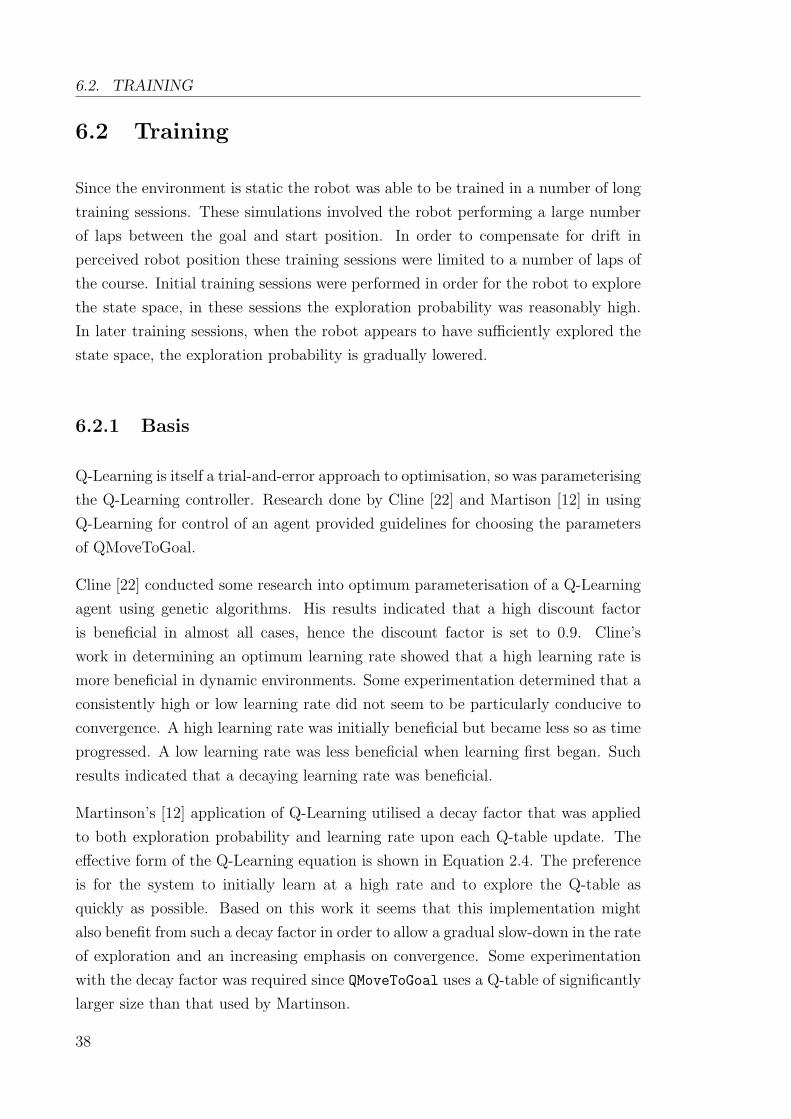
Since Q-learning is an on-line method of adaptation some experimentation with
reward functions and frequency of update was required in order to gauge acceptable
values. Cline’s [22] work in the area of tuning the Q-learning algorithm was used as
a basis when choosing the learning parameters for this system.
5.1.1 Task specification
In this case two implementations have been defined in the QMoveToGoal and QMove-
ToGoal2 controllers, both child classes of QLearningController. The task assigned
to both controllers was a navigation exercise, requiring the robot to drive between
two points in the environment without colliding with obstacles or getting stuck in
dead ends. Specification of the task was done via choice of state division and action
implementation. Careful choice of both reward functions determined which action
would eventually be chosen for a given state.
5.1.2 QMoveToGoal
State
The QMoveToGoal controller calculates current state based on obstacles detected in
the environment. This state is stored as an integer value, however it is assembled as
a sequence of codewords with each codeword representing the range detected by one
of the infrared sensors, in this case a position sensitive device (PSD). A range less
than 9999 (the maximum) is perceived as an obstacle and so the value is encoded
according to a certain resolution. In order to limit the size of the Q-values table
the resolution of each codeword is kept to a small number of bits. For the current
implementation of QMoveToGoal a two bit codeword is used for each PSD, the coding
scheme is given in table 5.1.
The current environmental state is given as the sequence of obstacle distance code-
words. These codewords are organised in sequence in a clockwise fashion starting
with the leftmost PSD in the most significant position. Equation 5.1 depicts the
codeword arrangement used in the current implementation, the example shown is
for when no obstacles are detected.
31

5.1. Q-LEARNING
Obstacle Distance (mm) Codeword> 2000 00> 1000 01> 500 10< 500 11
Table 5.1: Obstacle distance encoding scheme
State = 00︸︷︷︸(left)
00︸︷︷︸(front left)
00︸︷︷︸(front)
00︸︷︷︸(front right)
00︸︷︷︸(right)
010︸︷︷︸(octant of goal)
(5.1)
Action
The QMoveToGoal controller defines an action as the application of a set of weights
and parameters to the behavioural network. Each time the algorithm updates a new
set of weights and parameters are selected and applied. The QMoveToGoal controller
uses a set of schemas consisting of LinearAttractor, Noise and AvoidObstacles
(shown in Figure 5.3).
Move to Goal
Avoid Obstacles
Noise
detect goal
detect obstaclesmovement
vector
Figure 5.3: Behavioural assemblage used in the QMoveToGoal controller
As can be seen in Figure 5.3 QMoveToGoal only controls two variables, the Noise
schema weight and the sphere of influence of AvoidObstacles. The sphere of in-
fluence (of AvoidObstacles) determines the distance within which obstacles begin
to have a significant repulsion effect. These variables were chosen since it is not
necessary to modulate both the weight and sphere of influence of AvoidObstacles.
Significant reduction of the sphere of influence achieves the same goal as lowering
the weight, increasing the weight has little effect beyond a certain threshold as the
behaviour begins to dominate the output. The Noise weight is set to either a 0.5 or
0.0 weight in order to introduce randomness to the robot’s behaviour in the event
that it may be necessary.
32

CONTROLLER
The approach that this implementation is intended to take is known as ballooning.
The sphere of influence of avoid-obstacles is expanded, just as a balloon is in-
flated, in order to repel out of local minima. This approach was demonstrated by
Clark [18] in his work on learning momentum, however in this case the intent is to
use this approach to successful navigation of local minima by training the robot to
learn to employ it at the correct situation.
The alternative approach to ballooning is known as squeezing. In this technique the
sphere of influence of avoid-obstacles is reduced in order to squeeze through gaps
in barriers. Such a technique fails if the barrier has no gaps and so squeezing would
not be an optimal policy for all environments.
Reward
QMoveToGoal was created to complete a navigation exercise in which the robot would
move to its destination without colliding with obstacles or get stuck in local minima.
This problem definition required that positive reward be given for movement towards
the goal, but negative reward be given in the event of a collision.
In order to deter the robot from colliding with obstacles the reward function was de-
fined such that the robot receives negative reward. The robot receives an additional
reward equal to the change in collisions since last update. The reward due to colli-
sions is essentially rcollisions = (collisionsprevious−collisionscurrent)−collisionscurrent.
This reward accumulates quite rapidly in the event of a collision and so the robot
becomes averse to such action.
To satisfy the need of the robot to reach the goal the reward function adds an
additional reward based on the normalised movement in the direction of the goal.
This reward is calculated as rmovement = d.ml
, where d is the unit displacement to
goal, m is the displacement since last update and l is the length of the path since
last update. The divisor by the path length is used to lessen the reward in the event
that the robot does not take the shortest path between its previous and current
positions.
QMoveToGoal uses a slightly non-standard version of Q-Learning. At each iteration
of the algorithm, the learning rate and exploration probability exhibit a decay by a
certain amount. Decay is calculated as an exponential function, the base is taken
as 1 − d (where d is the decay) and the exponent increases with each iteration.
This decay was instituted in order to allow continuous simulation of the system and
33

5.1. Q-LEARNING
encourage early exploration of the state space. More information on this system is
given in Section 6.2.1.
5.1.3 QMoveToGoal2
The QMoveToGoal2 controller is a very similar implementation to that of its prede-
cessor. It does, however, take an alternative approach when it comes to state division
and action. The reward function is largely unchanged from that of QMoveToGoal.
State
Like QMoveToGoal this controller represents its state in a bit string. There are,
however, some differences. Most notable of these is that the number of states has
been greatly reduced. QMoveToGoal2 only takes into account whether or not an
obstacle is present in each of the directions, the definition of present being within
1000mm of the robot. This reduces the number of states down to 5 bits of object-
related state and 3 bits from the directional state, giving a total of 256 states for this
controller. The smaller number of states requires less training time since it requires
less time to explore the state space.
The reduction in state space size was done for two primary reasons. Firstly the
QMoveToGoal controller uses a large number of states and so requires significant ex-
ploration to cover the entire state space. Secondly, and perhaps most importantly,
not as many states are needed for this implementation. Since this controller takes a
different approach to the definition of an action it does not need any more informa-
tion about the environment than whether an obstacle is within a significant range
or not.
Action
QMoveToGoal2 takes an alternative approach to QMoveToGoal instead of choosing
an action from what is essentially a library of cases it chooses from a number of
possible actions. The actions in this case are distinct combinations of behaviours.
This implementation only performs three different actions: movement to goal, wall
following and repulsion/noise.
Wall-following is important in this implementation since it provides an alternate
approach to the ballooning strategy that QMoveToGoal is intended to employ. This
34

CONTROLLER
implementation has been designed in order to attempt to make the robot implement
navigation that resembles the Distbug [23] algorithm but does so in a behavioural
manner. The agent is intended to learn to trace the outline of obstacles when
they lie in such a wall that is beneficial to movement towards the goal. In other
circumstances the robot should act as if it was simply moving towards the goal.
5.2 Learning Momentum
One of the adaptive controllers that was implemented was based, in concept, on
the learning momentum technique presented by Clark [18]. This controller adapts
using a set of rules such that the robot encourages successful behaviours and dis-
courages unsuccessful ones. Learning momentum has been described previously in
Section 3.3.2. Learning momentum is a cheaper solution to implement as compared
to Q-Learning since it requires less overhead and no training time.
In learning momentum the controller functions according to a set of rules that eval-
uate based on environmental data and some measure of the internal state. An
implementation of a learning momentum-based framework was created, taking the
name LearningMomentumController. This controller allows derived classes to de-
fine their own set of rules to suit their particular behavioural network and desired
task.
The momentum element of this controller exists due to the nature of how rules
are applied. In Clark’s original implementation the rules caused an incremental
update of schema weights and parameters, thus the schema parameters did not
react instantaneously to a changing environment. In addition his implementation
averaged the environmental state thus providing a slowly changing average which
caused an additional inertia-like effect on schema weights. The implementation
created for this dissertation also utilises averaged environmental values, however the
LearningMomentumController only provides a framework for the implementation
of this technique. Hence it does not provide the averaging functionality since the
quantities to be averaged are determined by derived classes.
5.2.1 Rules
A controller to suit the same task as QMoveToGoal was created using a class derived
from LearningMomentumController. This controller, LMMoveToGoal, uses the same
35
5.2. LEARNING MOMENTUM
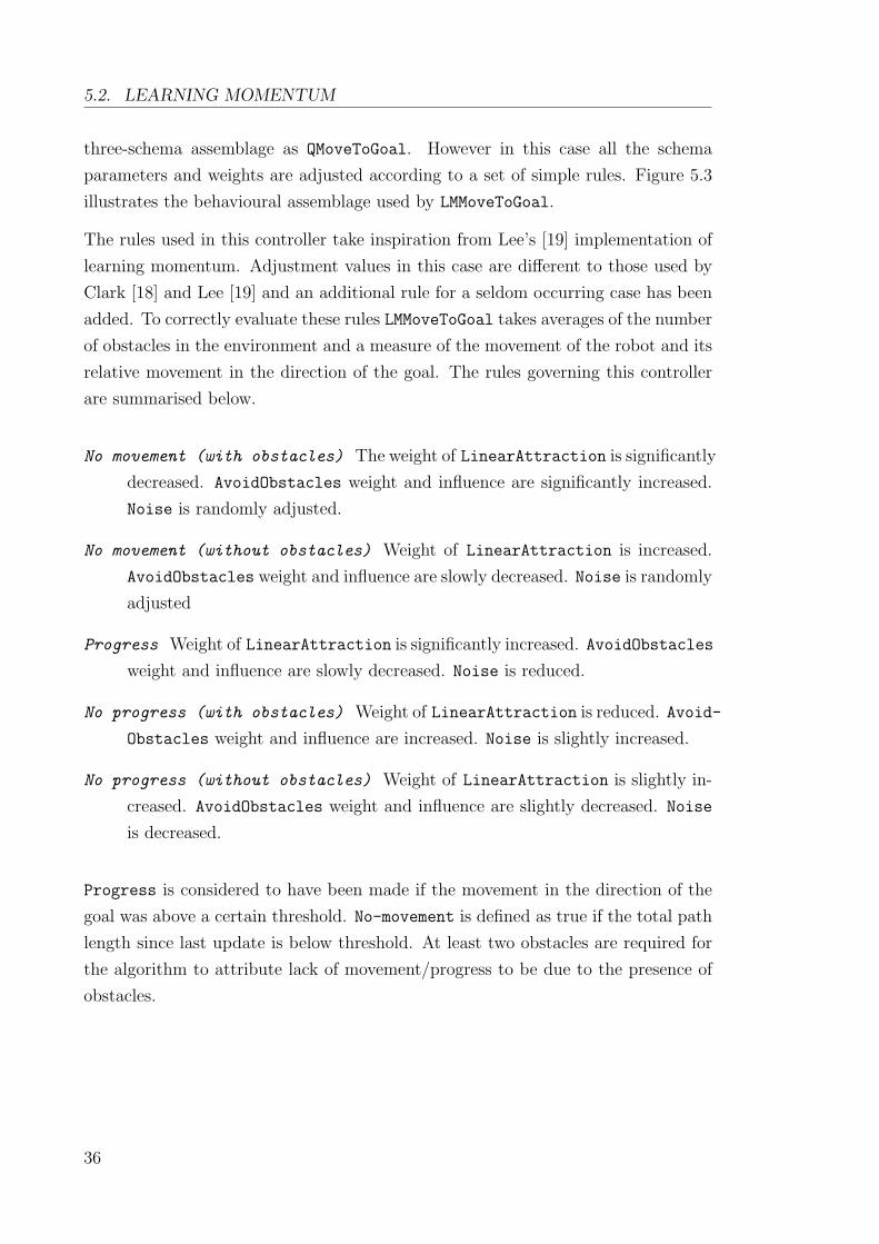
three-schema assemblage as QMoveToGoal. However in this case all the schema
parameters and weights are adjusted according to a set of simple rules. Figure 5.3
illustrates the behavioural assemblage used by LMMoveToGoal.
The rules used in this controller take inspiration from Lee’s [19] implementation of
learning momentum. Adjustment values in this case are different to those used by
Clark [18] and Lee [19] and an additional rule for a seldom occurring case has been
added. To correctly evaluate these rules LMMoveToGoal takes averages of the number
of obstacles in the environment and a measure of the movement of the robot and its
relative movement in the direction of the goal. The rules governing this controller
are summarised below.
No movement (with obstacles) The weight of LinearAttraction is significantly
decreased. AvoidObstacles weight and influence are significantly increased.
Noise is randomly adjusted.
No movement (without obstacles) Weight of LinearAttraction is increased.
AvoidObstacles weight and influence are slowly decreased. Noise is randomly
adjusted
Progress Weight of LinearAttraction is significantly increased. AvoidObstacles
weight and influence are slowly decreased. Noise is reduced.
No progress (with obstacles) Weight of LinearAttraction is reduced. Avoid-
Obstacles weight and influence are increased. Noise is slightly increased.
No progress (without obstacles) Weight of LinearAttraction is slightly in-
creased. AvoidObstacles weight and influence are slightly decreased. Noise
is decreased.
Progress is considered to have been made if the movement in the direction of the
goal was above a certain threshold. No-movement is defined as true if the total path
length since last update is below threshold. At least two obstacles are required for
the algorithm to attribute lack of movement/progress to be due to the presence of
obstacles.
36

Chapter 6
Navigation Task
6.1 Overview
Reinforcement learning, whilst an on-line adaptive technique, does require some
training of the agent before it will correctly interact with the environment. Train-
ing in simulation is preferred since it allows the agent full exploration of its state
space without the physical damage that can occur due to a wrong move. It also
allows easy definition of the training environment such that more constraints can be
incrementally introduced.
The QMoveToGoal adaptive controller (described in Section 5.1) required some train-
ing in order to perform its task. Training was conducted starting with a zero-
initialised table of Q-values. The robot was required to navigate through obstacle
fields of varying density in order to reach its goal. QMoveToGoal2 was also trained
in the same circumstances.
The trained controllers were evaluated by setting them the navigation task in a
number of environments of varying obstacle density. In order to provide some com-
parative measure of performance a learning-momentum-based controller and a con-
troller with static parameters were given the same task in the same environments.
All four controllers were given similar behavioural assemblages to use for this task
(see Figure 5.3).
37
6.2. TRAINING
6.2 Training
Since the environment is static the robot was able to be trained in a number of long
training sessions. These simulations involved the robot performing a large number
of laps between the goal and start position. In order to compensate for drift in
perceived robot position these training sessions were limited to a number of laps of
the course. Initial training sessions were performed in order for the robot to explore
the state space, in these sessions the exploration probability was reasonably high.
In later training sessions, when the robot appears to have sufficiently explored the
state space, the exploration probability is gradually lowered.
6.2.1 Basis
Q-Learning is itself a trial-and-error approach to optimisation, so was parameterising
the Q-Learning controller. Research done by Cline [22] and Martison [12] in using
Q-Learning for control of an agent provided guidelines for choosing the parameters
of QMoveToGoal.
Cline [22] conducted some research into optimum parameterisation of a Q-Learning
agent using genetic algorithms. His results indicated that a high discount factor
is beneficial in almost all cases, hence the discount factor is set to 0.9. Cline’s
work in determining an optimum learning rate showed that a high learning rate is
more beneficial in dynamic environments. Some experimentation determined that a
consistently high or low learning rate did not seem to be particularly conducive to
convergence. A high learning rate was initially beneficial but became less so as time
progressed. A low learning rate was less beneficial when learning first began. Such
results indicated that a decaying learning rate was beneficial.
Martinson’s [12] application of Q-Learning utilised a decay factor that was applied
to both exploration probability and learning rate upon each Q-table update. The
effective form of the Q-Learning equation is shown in Equation 2.4. The preference
is for the system to initially learn at a high rate and to explore the Q-table as
quickly as possible. Based on this work it seems that this implementation might
also benefit from such a decay factor in order to allow a gradual slow-down in the rate
of exploration and an increasing emphasis on convergence. Some experimentation
with the decay factor was required since QMoveToGoal uses a Q-table of significantly
larger size than that used by Martinson.
38

NAVIGATION TASK
In addition to the parameters of the Q-Learning equation the update frequency of
this system had to be chosen. Some experimentation was performed with regards
to this parameter and it was determined that retrieving a reward every 20 steps
allowed for sufficient movement for the rewards to be evaluated effectively. Further
experimentation determined that allocating reward when the state changed was a
more effective technique. However, since some actions can cause the robot to halt if
performed in the wrong state, it was decided that the controller should only remain
in one state without change of action for 20 steps. This approach is also more
appealing since it requires less parameterisation of the system. Actions which cause
the robot to halt should be discouraged before exploration ceases (and training is
complete).
The results of this experimentation are the parameters given in Table 6.1. The
form of the Q-Learning algorithm to use was the non-deterministic case (given in
Equation 2.4) which utilised a decay factor. Learning rate is initially set to 1.0,
discount factor is permanently set to 0.9. The exploration probability is initially set
to 0.55 and then a decay factor is applied to both the learning rate and exploration
probability of 0.00005 per iteration.
Parameter Valueα 1.0γ 0.9ε 0.55d 0.00005
Table 6.1: Parameters for the Q-Learning algorithm used in QMoveToGoal (given inEquation 2.4)
6.2.2 Regime
The training regime of the agent was chosen in order to give a higher probability
of successfully learning the desired parameters. Training of the agent is conducted
using parameters which are intended to improve the exploration of the state-action
table. In initial runs the exploration probability begins at 0.55, this is later decreased
as the robot appears to have explored the bulk of the Q-table. Initial learning
rate is set to 1.0 and the discount factor is permanently set to 0.9. After some
experimentation (see Section 6.2.1) the decay factor of the system is set to 5×10⁻⁵.
The training procedure for the agent was performed in a partially cluttered environ-
ment. The training environment is shown in Figure 6.1. The robot was required to
39

6.2. TRAINING
perform laps between the green and blue nodes, a lap is defined as the robot moving
from one node to the other and back again.
Figure 6.1: Training environment used for both the QMoveToGoal and QMoveToGoal2
controllers (destination is highlighted)
6.2.3 Analysis
The success of the training procedure is verified after the training procedure is
considered to be complete. The Q-Learning algorithm was expected to converge on
a solution after a sufficient number of laps. At this point the policy should not alter
and so training finishes. To measure the convergence of the system the learning rate
and exploration probability are allowed to decay to zero. The system then begins to
stabilise as no random element is occurring in the action selection process. Metrics
are then applied and a determination can be made whether the system is actually
converging on a solution.
To measure the convergence of the system a metric that counts the number of policy
changes per lap was used as the primary indicator. Policy changes indicate that the
system has not settled to the perceived optimal solution. Policy for the Q-Learning
controller is defined as the action for a given state that corresponds to the maximum
Q-value in that state. When the policy changes the maximum Q-value has changed
and so a different action would be selected from that state. Similarly the average
experienced reward should stabilise as time goes on since the system should select
the action it believes will generate the optimum reward each time.
The QMoveToGoal controller was applied to this environment for a number of laps
until the system appeared to converge on a solution. The policy changes per lap are
graphed in Figure 6.2. It can be seen that the number of policy changes decreases
in an approximately exponential curve. Reward experienced per lap is graphed in
Figure 6.3 and decays sharply. The large initial spikes in the graphs are due to the
40

NAVIGATION TASK
system engaging in large-scale exploration of its vast state space. Later peaks in
the number of policy changes may be attributed to hesitant behaviour whereby the
system oscillates between similar states with no optimal policy. These peaks may
also occur since the exploration of the state space is a random process.
2500
3000
3500
Ex
pe
rie
nce
d r
ew
ard
Experienced reward
-500
0
500
1000
1500
2000
2500
0 50 100 150 200 250
Ex
pe
rie
nce
d r
ew
ard
Lap
10000
Policy changes
0
1000
2000
3000
4000
5000
6000
7000
8000
9000
10000
0 50 100 150 200 250
Po
licy
ch
an
ge
s
Lap
Average policy changes
Average experienced reward
Figure 6.2: Graph of policy changes as training progresses for QMoveToGoal
2500
3000
3500
Ex
pe
rie
nce
d r
ew
ard
Experienced reward
-500
0
500
1000
1500
2000
2500
0 50 100 150 200 250
Ex
pe
rie
nce
d r
ew
ard
Lap
10000
Policy changes
0
1000
2000
3000
4000
5000
6000
7000
8000
9000
10000
0 50 100 150 200 250
Po
licy
ch
an
ge
s
Lap
Average policy changes
Average experienced reward
Figure 6.3: Graph of experienced reward as training progresses for QMoveToGoal
Unfortunately the results of the training indicate that the previously described im-
plementation of the QMoveToGoal controller utilises far too many states to effectively
use the Q-Learning algorithm. The algorithm can be seen to converge on an opti-
mal solution for a number of the states. However a large number of states remain
unvisited and on the occasion that they are visited a policy change ensues. These
41
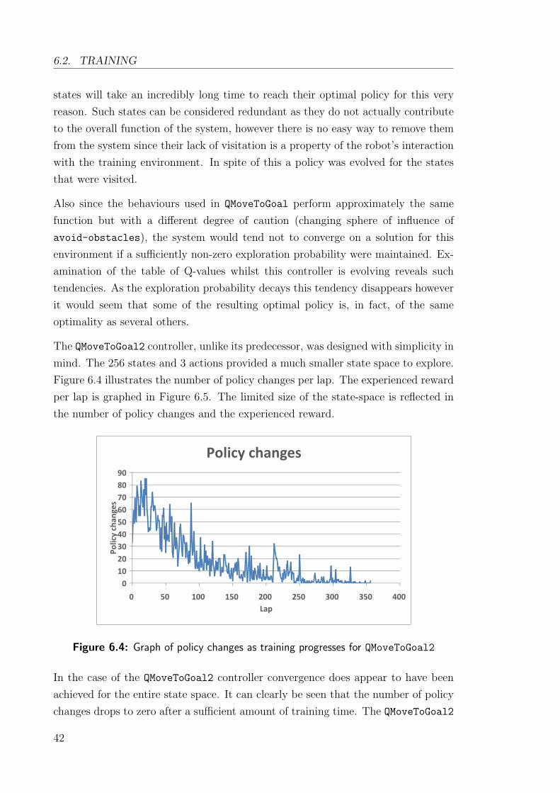
6.2. TRAINING
states will take an incredibly long time to reach their optimal policy for this very
reason. Such states can be considered redundant as they do not actually contribute
to the overall function of the system, however there is no easy way to remove them
from the system since their lack of visitation is a property of the robot’s interaction
with the training environment. In spite of this a policy was evolved for the states
that were visited.
Also since the behaviours used in QMoveToGoal perform approximately the same
function but with a different degree of caution (changing sphere of influence of
avoid-obstacles), the system would tend not to converge on a solution for this
environment if a sufficiently non-zero exploration probability were maintained. Ex-
amination of the table of Q-values whilst this controller is evolving reveals such
tendencies. As the exploration probability decays this tendency disappears however
it would seem that some of the resulting optimal policy is, in fact, of the same
optimality as several others.
The QMoveToGoal2 controller, unlike its predecessor, was designed with simplicity in
mind. The 256 states and 3 actions provided a much smaller state space to explore.
Figure 6.4 illustrates the number of policy changes per lap. The experienced reward
per lap is graphed in Figure 6.5. The limited size of the state-space is reflected in
the number of policy changes and the experienced reward.
40
50
60
70
80
90
Po
licy
ch
an
ge
s
Policy changes
200
250
Experienced reward
0
10
20
30
40
0 50 100 150 200 250 300 350 400
Po
licy
ch
an
ge
s
Lap
-50
0
50
100
150
200
0 50 100 150 200 250 300 350 400
Ex
pe
rie
nce
d r
ew
ard
Lap
Figure 6.4: Graph of policy changes as training progresses for QMoveToGoal2
In the case of the QMoveToGoal2 controller convergence does appear to have been
achieved for the entire state space. It can clearly be seen that the number of policy
changes drops to zero after a sufficient amount of training time. The QMoveToGoal2
42

NAVIGATION TASK
40
50
60
70
80
90
Po
licy
ch
an
ge
s
Policy changes
200
250
Experienced reward
0
10
20
30
40
0 50 100 150 200 250 300 350 400
Po
licy
ch
an
ge
s
Lap
-50
0
50
100
150
200
0 50 100 150 200 250 300 350 400
Ex
pe
rie
nce
d r
ew
ard
Lap
Figure 6.5: Graph of experienced reward as training progresses for QMoveToGoal2
controller appears to have an optimal solution for this training environment. The
occasional spike in the number of policy changes may be attributed to the prediction
mechanism failing due to misinterpretation of the current state. Successive policy
changes would ensue as the controller reverted to the optimal policy.
Even using such a limited number of states the QMoveToGoal2 controller only ex-
periences a certain number of the possible states. It is assumed that this is again
due to the construction of the environment. If the agent were to be trained in an
environment where obstacles only appeared on one side of the robot some of these
states are more likely to be explored. However in such an environment this controller
may be considered excessive.
The training process itself appears to be successful for the given QLearningController
implementations. Even so two key observations have been made as to the methods
involved, namely the reward function used and the concept of laps.
One of the elements of the problem that the reward function ignores is that no
reward is given when traversing the boundary of an obstacle that must be avoided.
If the path around that object takes the robot away from the main goal penalties can
be applied. This aspect of the reward function causes the flattening effect amongst
policies of similar optimality. Even so the reward function appears to be adequate
for the task.
Making the agent perform laps of the environment instead of restarting the simula-
tion at each lap may slightly perturb the results of the exercise. Upon reaching the
goal the robot must turn around to head to the new goal. At this point the robot is
43

6.3. COMPARISON TASK ENVIRONMENT
briefly heading in the wrong direction thus incurring penalty to the current policy.
This aberration is actually insignificant since the state at that point will be devoid
of obstacles and so the optimal policy is largely irrelevant given all available actions
perform similarly in such conditions.
6.3 Comparison Task Environment
To adequately evaluate the controllers a number of test environments were prepared.
These environments featured obstacles in varying configurations for the robot to
traverse. Three of the environments contained dead-ends from which the adaptive
controllers were tasked with escaping. The other environments simply provided
varying obstacle densities to see if a given controller would locate the quickest path
during traversal.
The robot that was used for these simulation trials was the S4X soccer robot, which
is provided with Eyesim. This robot was augmented with an additional two PSDs
placed to give readings to the front-left and front-right. These two additional PSDs
help to alleviate a possible blind-spot the typical three-PSD model can have when
navigation is based on PSD readings alone.
The behavioural assemblage used in all three controllers is given in Figure 5.3. This
assemblage is paired with the controllers as shown in Figure 5.2. This configuration
allows the controllers to modify both schema weights and parameters. The only
deviation from this assemblage occurs in the QMoveToGoal2 controller, in this case
the robot augments the assemblage with a wall-following behaviour. The wall-
following behaviour is only used in this case, the design of the other implementations
is such that they wouldn’t benefit from it.
This particular behavioural assemblage is chosen since it provides the functional-
ity required when moving between locations. Obviously the attraction behaviour
(move-to-goal) is necessary in order for the robot to consider approaching the
goal, likewise the avoid-obstacles behaviour is necessary so that the robot will
not crash. An additional component is required to introduce random perturba-
tions to provide the motivation for the robot to exit situations where deterministic
behaviour will lead to an endless loop. This schema is referred to as noise.
44

NAVIGATION TASK
6.4 Metrics
The various controllers have been evaluated using a number of metrics. The metrics
used are time taken, path length, number of collisions and total rotation. Since the
controllers are being evaluated in a software simulation all these quantities can be
measured with a good degree of accuracy.
Time taken and path length are obvious criteria by which to assess a controller.
It is preferable that in completing the task the robot performs efficiently and with
minimal cost. Time taken is measured in both simulator time and time in calculation
steps. Simulator time provides the actual time the robot took to reach the goal.
Time in calculation steps provides, when compared to actual time taken, a measure
of how calculation intensive each controller is.
Collisions per lap are measured since the robot is required to avoid collisions with
obstacles. The collisions measured are not actual collisions with the environment.
The framework tries to prevent the robot from colliding so a minimum safe distance
from obstacles is imposed. Whilst the robot remains at or within this minimum
safe distance any commands which may cause it to drive too close to obstacles are
ignored. Each cycle in which the robot remains at or within this distance is counted
as a collision.
Path length is used as a metric since it is preferred that the robot take the shortest
path and not make wasteful movements. Likewise the total rotation of the robot
is measured. The rationale for this is simple, rotations can be a costly operation
so the less rotation needed the more efficient the controller. In this framework a
rotation is performed simultaneously with a movement so rotation is costly since it
makes the movement less direct and will incur time and distance penalties.
6.5 Evaluation
The four controllers, MoveToGoal, LMMoveToGoal, QMoveToGoal, QMoveToGoal2,
were evaluated in the previously described task environments. The performance
of each controller has been averaged for each environment set in order to simplify
their display. Averaging the results of an entire environment set for each controller is
not an entirely feasible method of analysis for fine-grained analysis. However when
simply taking the relative performance of the control algorithms (in a general sense)
the averaging is valid.
45

6.5. EVALUATION
The results from testing these controllers over the task environments shows a re-
curring trend in all metrics used. The two Q-Learning based controllers took the
least time over environments where obstacles were present. QMoveToGoal proved to
be superior in the cluttered environment set, however it did not complete a number
of environments in the dead-end set. The statically weighted controller performs
most efficiently in an empty environment. In environments with a larger number of
obstacles static controller performance begins to degrade. LMMoveToGoal appears to
be an expensive alternative to use, however it is capable of successfully traversing
all environments.
6.5.1 Time
With regards to time, and hence speed, QMoveToGoal is the most time-efficient
of the controllers. However as can be seen in Figure 6.6 this controller fails to
make successful runs through dead-end environments. This is due to the controller
having evolved a very risk-friendly (ie. not particularly obstacle-averse) policy which
performs admirably in environments without local minima.
0102030405060708090
100
Free Cluttered Dead-end
Average path length
Static
Learning Momentum
QMoveToGoal
QMoveToGoal2
02000400060008000
100001200014000160001800020000
Free Cluttered Dead-end
Average time (steps)
Static
Learning Momentum
QMoveToGoal
QMoveToGoal2
0
200
400
600
800
1000
1200
1400
Free Cluttered Dead-end
Average rotation
Static
Learning Momentum
QMoveToGoal
QMoveToGoal2
Figure 6.6: Lap times for the various controllers averaged for environment sets
LMMoveToGoal tends to have the longest execution time of all the controllers. This
is largely due to the time taken to build momentum. It is also due to the bal-
looning strategy employed. When the robot expands the sphere of influence of the
avoid-obstacles schema it begins to take a wider, and hence more time consuming,
path through the environment. In the dead-end case MoveToGoal exceeds the exe-
46

NAVIGATION TASK
cution time of LMMoveToGoal. These scenarios were the criteria that LMMoveToGoal
was designed for, and so they offer improved performance with less reliance on noise.
The QMoveToGoal2 controller performs similarly well to QMoveToGoal, albeit using
a slightly more cautious approach that incurs a small additional time component.
However, unlike its predecessor, QMoveToGoal2 can escape from dead-end environ-
ments. Additionally, it is significantly faster than the statically weighted controller
since it relies less on noise. On average this controller would be considered to be
the most time-efficient of those evaluated.
6.5.2 Path Length
In Figure 6.7 the relative path length of the controllers for each environment set can
be seen to follow the same pattern as for time taken. There is a slight perturbation
to this in that the path lengths are more closely grouped than other measured values.
Overall QMoveToGoal2 offers a consistently close-to-minimal path length for varying
environmental conditions.
0102030405060708090
100
Free Cluttered Dead-end
Average path length
Static
Learning Momentum
QMoveToGoal
QMoveToGoal2
02000400060008000
100001200014000160001800020000
Free Cluttered Dead-end
Average time (steps)
Static
Learning Momentum
QMoveToGoal
QMoveToGoal2
0
200
400
600
800
1000
1200
1400
Free Cluttered Dead-end
Average rotation
Static
Learning Momentum
QMoveToGoal
QMoveToGoal2
Figure 6.7: Lap path lengths for the various controllers averaged for environment sets
In unconstrained environments the path lengths of the controllers are almost iden-
tical. This is to be expected since the avoid-obstacles schema only produces an
output if obstacles are detected. The only difference in the path lengths is due to
the noise component introduced by the LMMoveToGoal and QMoveToGoal controllers.
The difference in this environment set is so small that it can be ignored.
47

6.5. EVALUATION
Cluttered environments exhibit similar relative path lengths to relative time perfor-
mance. The learning-momentum based controller is, as usual, the slowest of those
compared. This would be due to its ballooning strategy that causes the robot to
circumnavigate the obstacle field. The other controllers offer similar performance by
entering and navigating through these fields. As in the time performance cases the
QMoveToGoal controller offers the minimal path since it is the least obstacle-averse.
The remaining controllers offer similar performance that is only sightly worse than
QMoveToGoal.
In the dead-end scenarios QMoveToGoal2 achieves a minimal path length. This
path length is only slightly shorter than that of LMMoveToGoal. Such performance
would suggest that the two algorithms are comparable in such scenarios, however
the LMMoveToGoal controller requires more time in order to adjust its parameters.
QMoveToGoal2 is only limited by the distance it takes to trace the outline of an
obstacle. A statically weighted controller requires far too much noise to escape local
minima to be of any practical use and unfortunately the QMoveToGoal controller
evolved a strategy that is simply unable to traverse dead-end environments.
6.5.3 Rotation
0102030405060708090
100
Free Cluttered Dead-end
Average path length
Static
Learning Momentum
QMoveToGoal
QMoveToGoal2
02000400060008000
100001200014000160001800020000
Free Cluttered Dead-end
Average time (steps)
Static
Learning Momentum
QMoveToGoal
QMoveToGoal2
0
200
400
600
800
1000
1200
1400
Free Cluttered Dead-end
Average rotation
Static
Learning Momentum
QMoveToGoal
QMoveToGoal2
Figure 6.8: Total rotation per lap for the various controllers averaged for environmentsets
It can be seen in Figure 6.8 that rotation follows the same trend as the other per-
formance indicators. LMMoveToGoal required a significant degree of rotation in the
process of changing its momentum. QMoveToGoal2 enters into a looping behaviour
48
NAVIGATION TASK
as it escapes dead-ends. The path trace of this behaviour will be examined in more
detail in Section 6.6. Schemas that are reliant on noise incur a significant degree of
rotation, hence the statically weighted controller performs abhorrently for dead-end
scenarios. Overall the QMoveToGoal2 controller is the most efficient when judged by
this metric. This is in accordance with other measurements.
6.5.4 Collisions
Comparison of the controllers with regards to the number of collisions per lap re-
veals that the QMoveToGoal2 controller, yet again, offers superior performance. An
unexpected result was that the statically weighted controller actually incurred col-
lisions in some scenarios. This can occur if the robot approaches an obstacle on an
angle and the obstacle is of a size such that it is not detected by other PSDs until
it is near to the robot. The only controller that collides a significant number of
times is LMMoveToGoal and this is due to the way in which momentum is built and
lost. Whilst QMoveToGoal2 performs most successfully for this metric it does not
accurately reflect the performance of all the controllers.
6.6 Paths
Examination of the paths traced by the controllers provides an alternative method
of describing their performance. The features that characterise these path traces can
be used to generate a generalised prediction for the performance of each controller. A
selection of the task environments have been chosen and the controller performance
and path features in these scenarios are discussed.
6.6.1 Cluttered environments
Two of the cluttered scenarios can be used to give a general overview of controller
performance. One of the scenarios used is similar to a dead-end scenario with a minor
yet significant difference. The other example is simply a cluttered environment in
which certain features of the paths taken by each controller are more distinct.
49

6.6. PATHS
Scenario One
For this environment the QMoveToGoal controller was the most efficient. In Fig-
ure 6.9 it can be seen that this controller is a lot less obstacle-averse than other
controllers. It maintains a smaller distance from the wall thus allowing it to squeeze
through gaps. There are no particularly novel features in the path trace for this
controller although the benefit of the squeezing strategy in this environment is ob-
vious.
-4
-3
-2
-1
0
1
2-4 -3 -2 -1 0 1 2
LMMoveToGoal
QMoveToGoal
QMoveToGoal2
MoveToGoal
Figure 6.9: Path traces for each controller in cluttered environment one
QMoveToGoal2 performed similarly to its predecessor. The only difference, apart
from the increased safety margin, is the loop that occurs when the robot attempts
to enter the gap in the wall. This looping behaviour is an unexpected side effect of
the choice of behaviours and evolved policy. It is produced as a side effect of the
wall-following schema attaching to the wall and the policy changing slightly too
late for the robot to enter the gap. The policy then dictates that the robot disengage
from the wall and the loop is performed to enter the gap. This looping behaviour
becomes more prevalent in dead-end scenarios.
In this scenario both of the reference controllers trace out the longest paths. The
statically weighted controller consistently misinterpreted the wall and followed it
in the wrong direction initially. It is unclear why this set of behavioural parame-
ters would differ so significantly from that of QMoveToGoal2 in this particular case.
LMMoveToGoal simply misinterprets the environment as being a dead-end scenario.
Neither of the reference controllers offer consistently the same performance as those
that were evolved.
50

NAVIGATION TASK
Scenario Two
In this environment the QMoveToGoal controller was again the most efficient. The
squeezing strategy it adopts allows it to fit between gaps that other controllers would
be repelled by. Whilst this strategy is not the policy that was originally desired it
does perform admirably in environments such as this.
-5
-4
-3
-2
-1
0
-3 -2 -1 0 1 2
LMMoveToGoal
QMoveToGoal
QMoveToGoal2
MoveToGoal
Figure 6.10: Path traces for each controller in cluttered environment two
Observation of Figure 6.10 indicates that the policy evolved by QMoveToGoal2 is
identical in performance to MoveToGoal in this scenario. Given the set of actions
available to the trained controller this is in fact the desired behaviour in such cir-
cumstances. Such performance would suggest the success of the training process for
QMoveToGoal2.
LMMoveToGoal performs, as it usually does, quite badly in such circumstances. This
controller was designed purely to escape local minima. In this scenario there is no
local minima present. It does appear that this controller adopts a squeezing policy,
however what actually happened was that at the first corner the robot encountered
the obstacle and lost momentum. It then began to build up momentum again and
moved towards the goal while experiencing increasing levels of repulsion from ob-
stacles, thus exhibiting the slingshot style movement out of and around the obstacle
field.
51

6.6. PATHS
6.6.2 Dead-end environments
The controllers were evaluated in a number of dead-end environments. Two have
been chosen to describe the performance of the controllers in such situations. The
first scenario is less typical since it can be considered somewhat of a special case.
The second scenario is a good example of a difficult to navigate dead end.
Scenario One
The scenario illustrated in Figure 6.11 is something of a special case. If the angle of
the barrier is made more acute then it becomes a far more difficult obstacle. As it
stands, this scenario was traversable by all controllers.
-3.5
-2.5
-1.5
-0.5
0.5
1.5 -1 0 1 2 3 4
LMMoveToGoal
QMoveToGoal
QMoveToGoal2
MoveToGoal
Figure 6.11: Path traces for each controller in dead-end scenario one
In this scenario the QMoveToGoal2 controller performed as expected. It did not ex-
hibit any of its characteristic looping behaviour due to the simple nature of the ob-
stacle field. The policy evolved by this controller performs optimally out of the four
controllers for this particular environment. Both QMoveToGoal and MoveToGoal ex-
hibit similar behaviour albeit with some confusion when approaching the apex of the
obstacle. This confusion lead to slightly lesser performance than the QMoveToGoal2
controller.
The reference controller LMMoveToGoal performed its typical action of losing and
re-establishing momentum. In such an environment this is unnecessary and lead to
an unnecessarily long path. However if the barrier were to be made more acute then
this strategy would be quite sound.
52

NAVIGATION TASK
Scenario Two
Figure 6.12 describes a dead-end scenario that is similar to that given in Figure 6.9.
QMoveToGoal was unable to traverse this scenario since the squeezing strategy causes
it to become trapped in local minima such as this. Likewise, MoveToGoal would nor-
mally become trapped in such an environment. A modified version of the statically
weighted controller was used for this scenario. The parameterisation used in this
case used a heavy weighting for the noise schema in order to allow it to escape the
trap. Due to the exceedingly high levels of noise the path taken can vary wildly.
One of the paths this controller took is presented here to provide a reference of
performance for the adaptive controllers. It can be seen that MoveToGoal is, whilst
successful, an untenable solution given its almost entirely random nature.
-6
-5
-4
-3
-2
-1
0
1
2-4 -3 -2 -1 0 1 2 3 4
LMMoveToGoal
QMoveToGoal2
MoveToGoal
Figure 6.12: Path traces for each controller in dead-end scenario two
In this scenario both QMoveToGoal2 and LMMoveToGoal can be considered the most
successful. LMMoveToGoal actually traverses the environment in the shortest path.
It does, however, take the longest time due to the process involved in losing and
building up momentum to escape the trap. QMoveToGoal2 on the other hand, traces
out a slightly longer path. It does so in, on average, less time and with less rotation.
QMoveToGoal2 is also preferred since it consistently produces similar results. The
reference controller is far less predictable due to the random elements involved in
applying rules.
An interesting feature of the QMoveToGoal2 controller is the looping pattern that
emerges as it begins to exit the trap. This behaviour was definitely not designed into
the system and so can be considered emergent. It can be clearly seen in Figure 6.12
that the agent tries to follow the wall but begins to veer away from it. This deviation
53

6.7. EVOLUTION ANALYSIS
would be due to the output of the move-to-goal schema attempting to turn the
robot to the goal node. The controller locks on to the wall and eventually gets pulled
away, however it loops around and reattaches. The explanation for this phenomenon
is difficult since the design of the behaviours involved would suggest that it had lost
the lock on the wall and would simply attempt to head towards the goal. It would
appear that the evolved policy causes QMoveToGoal2 to succeed where it otherwise
might no have.
6.7 Evolution Analysis
Results of the trials indicate that the QMoveToGoal controller did not evolve in
the intended manner. Instead of performing a ballooning strategy of navigation,
whereby the stuck agent escapes traps by expanding the region in which it is repelled
by obstacles, the controller appears to have learnt a squeezing strategy. In this
strategy the agent attempts to navigate the world via squeezing between obstacles,
this technique will not work for dead end scenarios although it does provide the
shortest path through some of the partially cluttered environments.
The shortcomings of QMoveToGoal can most likely be attributed to an insufficient
reward function and, possibly, an insufficient action set. Also, given a different
reward function a training environment catering to the desired mode of operation
should have been used. Additionally QMoveToGoal uses far too may states too be
practical, and it appears that having a large number of states is not in fact beneficial.
However the QMoveToGoal has chosen a policy that is consistent with the reward
function it trained with. Analysis of the paths this controller takes indicates that it
offers significantly improved performance in scenarios that are not dead-ends.
QMoveToGoal2, on the other hand, appears to have evolved the correct policy that it
was intended to perform. This algorithm has a slight advantage since it was select-
ing distinct actions that were behavioural combinations known to perform certain
functions. However the wall-following behaviour when used alone has a tendency
to seek corners (thus getting stuck) and so the policy is necessary for successful nav-
igation to the goal. The evolved policy adds some unexpected behaviour due to the
nature of the policy that was evolved. Fortunately the looping behaviour appears
to be either benign or beneficial.
The QMoveToGoal2 controller evolved a policy that is successful for the environments
presented. Successful performance would suggest that the controller has a valid set
54

NAVIGATION TASK
of actions and an appropriate reward function. Examination of the table of Q-values
for this controller indicates that a number of states remain unvisited and so state
assignment could be further simplified. Regardless of this inefficiency QMoveToGoal2
has been demonstrated to address the shortcomings of the other adaptive controllers
in performing the desired task.
55

56

Chapter 7
Conclusion
7.1 Behaviour based frameworks
The aim of this project was the design and implementation of a software framework
for the development of behaviour based applications for autonomous mobile robots.
Two frameworks have been implemented in order to represent both of the dominant
architectures in the field, AuRA and subsumption. Both frameworks have been
supplied with a number of simple behaviours and various primitives in order to
facilitate application development.
The primary framework, with an architecture based on AuRA, provides for the
development of applications using behaviours that can be represented by vector
fields. The current implementation of this framework provides interfaces for the
development of new behaviours as well as the expansion of the system controller.
The controller currently possesses a limited interface allowing the passing of goals
into the system. Extension of this interface could allow the use of a higher level
deliberative planner to bootstrap the reactive subsystem.
The secondary framework, based on subsumption, implements behaviour based con-
trol through the combination of behaviours designed to mimic the interconnectivity
of hardware modules. This framework provides a number of behavioural modules
which implement a basic layer of self-preservation behaviour and some simple tasks.
The implementation of this framework was such that it is lightweight and has been
deployed successfully to an Eyebot mobile robot.
57

7.2. ADAPTIVE CONTROLLERS
7.2 Adaptive controllers
Interfaces for adaptive controllers to extend the primary framework have been de-
veloped. An adaptive controller allows applications created by this framework to
act in a more robust way and allows for some degree of self-optimisation without
designer intervention. In this framework two controllers have been developed that
allow on-line adaptation.
The Q-Learning algorithm was chosen as a basis for adaptive control. This algorithm
has been applied in two different methods in order to evolve an improved controller
for navigation of an obstacle field. The controllers were evolved by setting them a
navigation task which they performed repeatedly in a specially constructed training
environment. Since the agents adapt on-line the training process was automated
and continued until convergence metrics were deemed to have reached acceptable
thresholds. During training it was possible to watch the agent performance improve
in real-time.
Evolution of the controllers produced mixed results. The first controller to be
evolved adopted a policy that generally satisfied the reward function it was trained
with. However, in dead-end scenarios the evolved policy was useless since it achieved
its goals using a policy almost the opposite of that intended. In other scenarios the
policy is quite efficient. The second controller evolved adopted a policy that al-
most exactly matched the desired criteria. While some unexpected behaviour can
be observed during execution it still performs the specified task. Such differences in
outcomes of the evolution process suggest care must be taken when selecting states,
actions and reward functions in order to correctly define the problem and desired
behaviour. While the current implementation will converge on a policy, this may
not be the policy intended by the designer.
7.3 Future Work
The frameworks that have been developed in this project may be used as a basis for
further work in the area of behavioural robotics. Both frameworks have a limited set
of behaviours available and could benefit from an extension of their libraries. These
frameworks could also be extended by the creation of a graphical user interface
for the definition of controllers or combination of behavioural modules. Such an
interface would simplify the creation of behaviour based applications.
58

CONCLUSION
Controllers developed for the primary framework are currently descended from a
simple controller definition. Future work could extend this controller definition to
allow bootstrapping of the reactive controller with goals of arbitrary type rather than
only passing positional goals as it does now. Currently the controller specification
defines success and failure codes so that the reactive subsystem can interact with a
higher level deliberate planner. Such a planner has not yet been implemented. The
creation of a planner and its fusion with the reactive subsystem could create a more
robust platform. This would add the capabilities to perform complex multistage
tasks in a behaviour based mode, of analysing environmental data and generating
alternate plans in the case of failure.
Finally, the current suite of adaptive controllers is limited to two on-line adap-
tive techniques. Future work could involve extending this suite to include off-line
techniques such as a neural network controller or one that learns using a genetic
algorithm. Whilst off-line adaptive techniques do not offer performance gains in
situ using a neural network offers the capability to generalise a solution.
59

60
Appendix A
Primary Framework
A.1 Overview
In this framework robot behaviour is created by combining the outputs of motor
schemas. Motor schemas are the essential units of behaviour. Behaviours are imple-
mented by creating classes derived from class MotorSchema. Motor schemas input
in order to function; this can be from either a perceptual schema or the result of a
network of schemas. Schemas are all derived from the class Node.
A.2 Creating behaviour
All schemas are of type Node. Schemas that take input from another schema require
the capability to evaluate their input. Classes derived from the root were created in
order to provide evaluation in their base data type. The primitive elements listed
below all provide a basic data type as their output. Their hierarchical arrangement
can be seen in Figure A.1. All these classes reside in the behaviour namespace
defined in node.h.
The list below includes the MotorSchema and PerceptualSchema classes. These
classes provide some additional functionality for creating behaviours and sensory
processing nodes. The use of either of these classes is not strictly required by the
framework if alternate controllers are to be used, however the included controllers
all consider them necessary.
When building a network of schemas some operator nodes may be used to process
data. These nodes are intended for use when some combination or processing of
61

A.2. CREATING BEHAVIOUR
data might be needed prior to its use as a schema input. A listing of the operator
nodes is provided.
A.2.1 Primitive types
behaviour::Node
behaviour::NodeBoolean
behaviour::NodeDouble
behaviour::NodeHSVImage
behaviour::NodeImage
behaviour::NodeInt
behaviour::NodeRGBImage
behaviour::NodeScalar behaviour::NodeVector2
behaviour::MotorSchema
behaviour::PerceptualSchema
Figure A.1: Class hierarchy of the primitive types of the framework
Node: Root node of the class hierarchy, provides a basis from which to derive other
types.
NodeScalar: Basis of the scalar types.
NodeInt: Node type that evaluates as an integer.
NodeDouble: Node type that evaluates as a double.
NodeBool: Node type that evaluates as a boolean.
NodeVector2: Node type that evaluates as a Vector2.
MotorSchema: Base type for all motor schemas. This class provides the framework
evaluating the success or failure of a behaviour.
PerceptualSchema: Base type for all schemas that perform sensory processing.
Provides the functionality of a list so multiple targets may be returned.
NodeImage: Node type that evaluates as an Image.
62
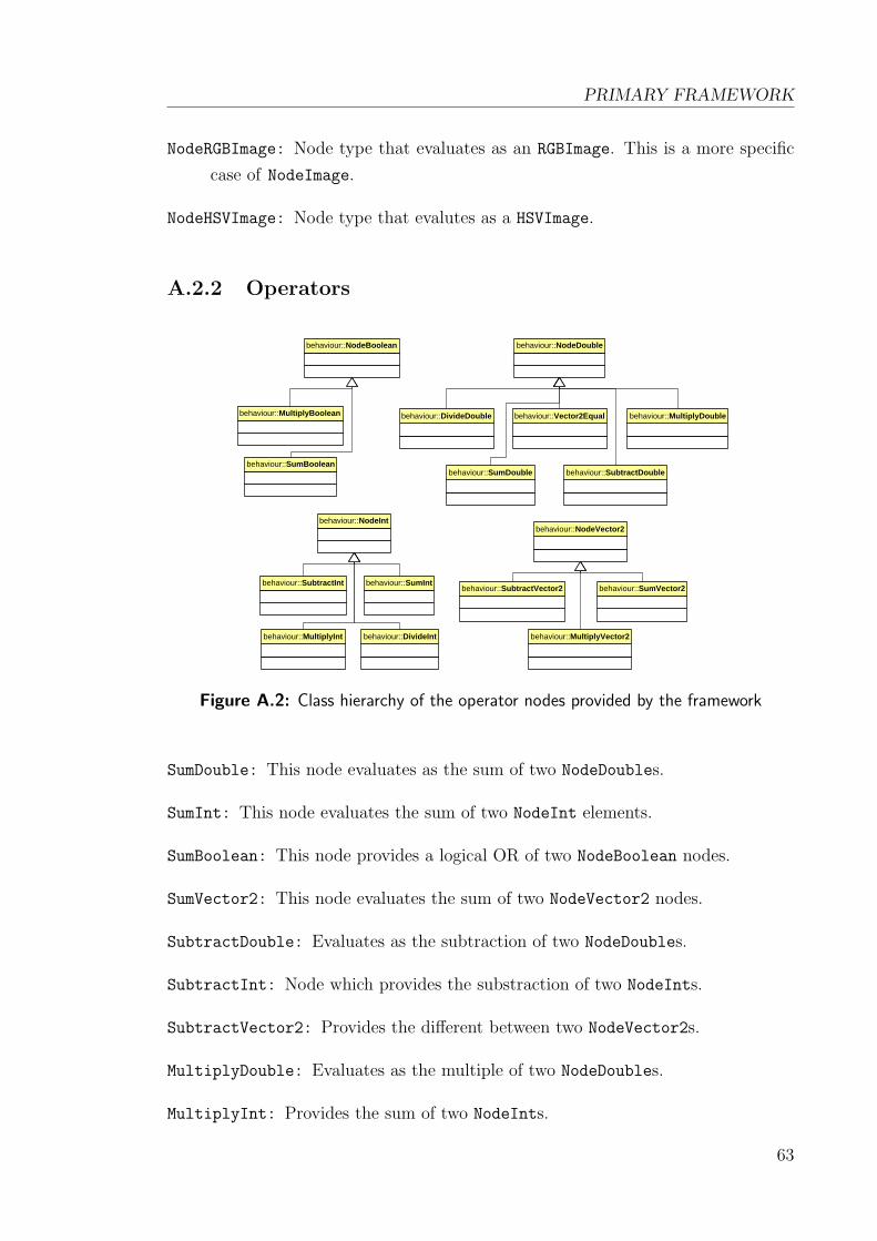
PRIMARY FRAMEWORK
NodeRGBImage: Node type that evaluates as an RGBImage. This is a more specific
case of NodeImage.
NodeHSVImage: Node type that evalutes as a HSVImage.
A.2.2 Operators
behaviour::SumBooleanbehaviour::SumDouble
behaviour::SumIntbehaviour::SumVector2behaviour::SubtractVector2
behaviour::SubtractInt
behaviour::SubtractDouble
behaviour::Vector2Equal
behaviour::MultiplyVector2behaviour::MultiplyInt
behaviour::MultiplyDoublebehaviour::MultiplyBoolean behaviour::DivideDouble
behaviour::DivideInt
behaviour::NodeBoolean behaviour::NodeDouble
behaviour::NodeIntbehaviour::NodeVector2
Figure A.2: Class hierarchy of the operator nodes provided by the framework
SumDouble: This node evaluates as the sum of two NodeDoubles.
SumInt: This node evaluates the sum of two NodeInt elements.
SumBoolean: This node provides a logical OR of two NodeBoolean nodes.
SumVector2: This node evaluates the sum of two NodeVector2 nodes.
SubtractDouble: Evaluates as the subtraction of two NodeDoubles.
SubtractInt: Node which provides the substraction of two NodeInts.
SubtractVector2: Provides the different between two NodeVector2s.
MultiplyDouble: Evaluates as the multiple of two NodeDoubles.
MultiplyInt: Provides the sum of two NodeInts.
63
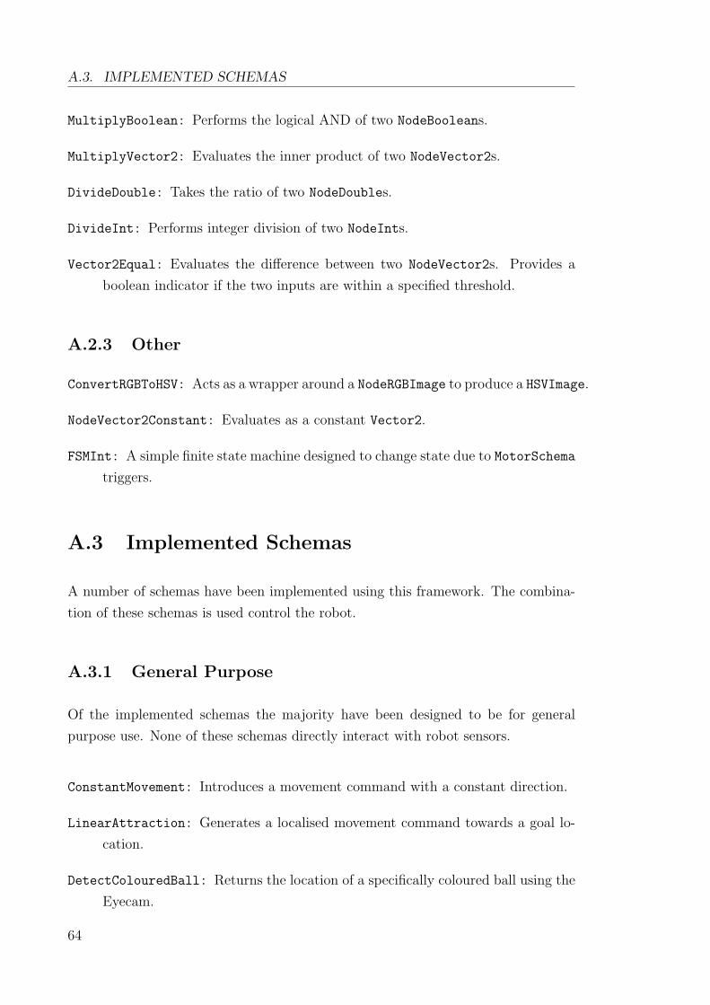
A.3. IMPLEMENTED SCHEMAS
MultiplyBoolean: Performs the logical AND of two NodeBooleans.
MultiplyVector2: Evaluates the inner product of two NodeVector2s.
DivideDouble: Takes the ratio of two NodeDoubles.
DivideInt: Performs integer division of two NodeInts.
Vector2Equal: Evaluates the difference between two NodeVector2s. Provides a
boolean indicator if the two inputs are within a specified threshold.
A.2.3 Other
ConvertRGBToHSV: Acts as a wrapper around a NodeRGBImage to produce a HSVImage.
NodeVector2Constant: Evaluates as a constant Vector2.
FSMInt: A simple finite state machine designed to change state due to MotorSchema
triggers.
A.3 Implemented Schemas
A number of schemas have been implemented using this framework. The combina-
tion of these schemas is used control the robot.
A.3.1 General Purpose
Of the implemented schemas the majority have been designed to be for general
purpose use. None of these schemas directly interact with robot sensors.
ConstantMovement: Introduces a movement command with a constant direction.
LinearAttraction: Generates a localised movement command towards a goal lo-
cation.
DetectColouredBall: Returns the location of a specifically coloured ball using the
Eyecam.
64

PRIMARY FRAMEWORK
behaviour::AvoidObstacles behaviour::ApproachClosestTarget
behaviour::ConstantMovement
behaviour::LinearAttractionbehaviour::LinearRepulsion
behaviour::Noise behaviour::IntervalNoise
behaviour::MotorSchema behaviour::DetectColouredBall
behaviour::FollowWalls
behaviour::ReachedColouredBall
Figure A.3: Hierarchy of the general purpose motor schemas created for the framework
ReachedColouredBall: A motor schema that is intended for use as a trigger to de-
termine whether a coloured object is close enough. Relies on some assumptions
about the environment.
ApproachClosestTarget: Generates a localised movement command towards the
closest target provided by a PerceptualSchema.
FollowWalls: Enables a wall following behaviour at a specified distance.
AvoidObstacles: Avoids obstacles within a specified distance.
LinearRepulsion: Generates a localised movement command away from a loca-
tion.
Noise: Movement commands randomly generated by a random process.
IntervalNoise: Movement commands periodically generated by a random process.
A.3.2 EyeBot Specific
These schemas are used to read and process sensory data from the Eyebot family of
mobile robots.
EyebotPSDLeft: Returns an integer reading from the left Eyebot PSD.
EyebotPSDRight: Returns an integer reading from the right Eyebot PSD.
EyebotPSDFront: Returns an integer reading from the front Eyebot PSD.
EyebotGlobalPosition: Returns the global Eyebot position as a vector.
65

A.4. CONTROLLER HIERARCHY
behaviour::PerceptualSchema
eyebot_sensors::EyebotDetectObstacles
eyebot_sensors::EyebotGlobalOrientation
eyebot_sensors::EyebotGlobalPosition
eyebot_sensors::EyebotPSDFront
eyebot_sensors::EyebotPSDLeft
eyebot_sensors::EyebotPSDRight
eyebot_sensors::EyecamGreyscale
eyebot_sensors::EyecamRGB
behaviour::NodeIntbehaviour::NodeImage
behaviour::NodeRGBImage
Figure A.4: Class hierarchy of the Eyebot-specific schemas
EyebotGlobalOrientation: Returns the global Eyebot orientation expressed as a
unit vector.
EyebotDetectObstacles: Provides a list of detected obstacle positions in local
coordinates.
EyecamGreyscale: Returns a greyscale Image from the Eyebot camera.
EyecamRGB: Returns an RGBImage from the Eyebot camera.
A.4 Controller Hierarchy
A hierarchy of controllers which provide layers of functionality have been developed
with the framework. The controller class hierarchy diagram is given in Figure A.5.
A.4.1 SimpleEyebotController
This controller provides the basic functionality that all others build upon. The
schemas in a SimpleEyebotController are combined in a weighted sum using a
static set of weights dependent on the current state of the controller. The controller
is built around a finite state machine which tracks the state and schema weights.
The FSM is triggered by the status of MotorSchemas. States, weights and triggers
are definable in a class which implements a constructor for this controller.
66
PRIMARY FRAMEWORK
controller::VirtualController
controller::EyebotController
controller::SimpleEyebotController
controller::AdaptiveEyebotController
controller::LearningMomentumControllercontroller::QLearningController
controller::QMoveToGoal
controller::SimpleMoveToGoalcontroller::SimpleLocateBall
behaviour::Nodebehaviour::FSMInt
virtual_robot::Eyebot
Figure A.5: Class hierarchy of the framework controllers
A.4.2 AdapativeEyebotController
The AdaptiveEyebotController is an interface intended to add in updates to the
system upon each calculation step.
A.4.3 QLearningEyebotController
This controller extends the adaptive capabilities to have on-line adaptation based
around the Q-Learning algorithm. The controller is used by specifying a constructor
and defining states and actions.
A.4.4 LearningMomentumController
This adaptive controller adds the capability to adjust the system using the learning
momentum algorithm.
A.5 Sample Program: Ball-finding example
The sample program given in Listing A.5 implements a simple ball-finding task.
This example uses the SimpleLocateBall controller, the listing for this controller
can be found on the enclosed DVD.
67

A.5. SAMPLE PROGRAM: BALL-FINDING EXAMPLE
This example demonstrates instantiation of a controller and looping until the con-
troller returns an abnormal status signal. Such a signal may be returned if the
controller detects the mission is complete or in the case of failure or other errors.
The SimpleLocateBall controller that is used in this example will always return
the MISSION OK signal.
When this example program is executed the robot will proceed to search for objects
on screen of the correct hue. In Listing A.5 the robot searches for a hue of zero, that
is the colour red. This example will also avoid obstacles that are within 350mm of
the robot.
#include "example_eyebot_controller.h"
int main(int argc, char **argv)
{
srand(time(NULL));
virtual_robot::Eyebot robot(0);
LCDPrintf("Press any key to begin..\n");
KEYWait(ANYKEY);
LCDClear();
/* Single controller detect ball example */
controller::SimpleLocateBall c(&robot, 0, 350);
while(c.step() == controller::MISSION_OK);
return 0;
}
Listing A.1: Example of a ball-finding program implemented in this framework
68
Appendix B
Subsumption Framework
B.1 Appendix for the Subsumption Framework
In this framework robot behaviour is created by connecting behavioural modules.
This implementation is built around the SubsumptionBuffer class. The buffers
produce an output which other buffers can use. Actuation and sensing is performed
by buffers designed for this purpose.
B.2 Creating behaviour
Behaviour is created using a network of behavioural modules. In this framework
these modules are termed ‘buffers’. Each buffer takes a number of inputs and has a
defined output and a signalling output. The signalling output is true if the module
is intending to signal an output value.
This framework provides a number of base buffers which output various data types.
These buffers are intended to be simple to combine and use. Their class hierarchy
has been illustrated in Figure B.1.
B.2.1 Buffers
Buffers of the following types are defined by the framework.
69

B.2. CREATING BEHAVIOUR
behaviour::SubsumptionBuffer
behaviour::SubsumptionBufferBool
behaviour::SubsumptionBufferDouble
behaviour::SubsumptionBufferInteger
behaviour::SubsumptionBufferVector2
behaviour::SubsumptionBufferVector2List
behaviour::SubsumptionSupressor
behaviour::SubsumptionSupressorBool
behaviour::SubsumptionSupressorDouble
behaviour::SubsumptionSupressorInteger
behaviour::SubsumptionSupressorVector2
Figure B.1: Class hierarchy of the framework SubsumptionBuffer classes as well asthe suppressor classes.
SubsumptionBuffer: Base subsumption buffer class.
SubsumptionBufferDouble: Subsumption buffer that generates an output of type
double.
SubsumptionBufferBool: Subsumption buffer with a boolean output.
SubsumptionBufferInteger: Subsumption buffer with an output of integer type.
SubsumptionBufferVector2: Subsumption buffer with a vector output.
SubsumptionBufferVector2List: Buffer which provides a list of vectors as the
output.
B.2.2 Supressors
Supressor buffers take input from two other buffers. One of the buffers is defined as
the primary signal and will override the other if it is signalling. If it is not then the
output is set to that of the alternate signal. Supressor buffers are used to include
additional layers of functionality. Lower layers will suppress higher layers.
SubsumptionSupressor: Interface which provides the suppressive functionality.
SubsumptionSupressorDouble: Suppressive buffer which works with Subsumption-
BufferDouble.
70

SUBSUMPTION FRAMEWORK
SubsumptionSupressorInteger: Subsumption buffer which uses SubsumptionSupressor-
Integer types.
SubsumptionSupressorBool: Buffer which takes two SubsumptionBufferBools.
SubsumptionSupressorVector2: Suppressive that works with SubsumptionBuffer-
Vector2s.
B.2.3 Inhibitors
Inhibitor buffers perform the mostly the same functionality as suppressive ones. The
only difference is that if the primary signal is signalling then the output of the buffer
is a zero.
behaviour::SubsumptionBufferBool
behaviour::SubsumptionBufferDouble
behaviour::SubsumptionBufferInteger
behaviour::SubsumptionBufferVector2
behaviour::SubsumptionInhibitorBool
behaviour::SubsumptionInhibitorDouble
behaviour::SubsumptionInhibitorInteger
behaviour::SubsumptionInhibitorVector2
behaviour::SubsumptionInhibitor
behaviour::SubsumptionSupressor
Figure B.2: Class hierarchy of the inhibitive classes
SubsumptionInhibitor: Interface which provides the suppressive functionality.
SubsumptionInhibitorDouble: Inhibitive buffer which works with Subsumption-
BufferDouble.
SubsumptionInhibitorInteger: Integer-valued inhibitive buffer.
SubsumptionInhibitorBool: Boolean-valued inhibitive buffer.
71

B.3. BEHAVIOURAL MODULES
B.3 Behavioural Modules
Several behavioural modules have been implemented using this framework. The
majority of these modules are designed to performed functionality mentioned in
Brooks’ [4] original design.
B.3.1 General purpose
The behavioural modules (Figure B.3) that have been implemented have been de-
signed for general purpose use. These buffers are all robot-independent. In general
these buffers are descendents of the SubsumptionBufferDouble types.
behaviour::AngleToGoal
behaviour::Collide
behaviour::Feelforce
behaviour::Noisebehaviour::RunAway
behaviour::Target
behaviour::Wander
behaviour::WallFollowingbehaviour::Closer
behaviour::SubsumptionBufferBoolbehaviour::SubsumptionBufferDouble
behaviour::SubsumptionBufferVector2
Figure B.3: Class hierarchy of the implemented behavioural modules
Collide: Collide is of boolean type and indicates whether or not a collision is
imminent.
Feelforce: Returns a vector representing a repulsive force away from obstacles.
RunAway: Signals a turn angle if a significant force is detected. In case of a collision
an about turn is executed.
Noise: Randomly generates an angle to turn.
Wander: Periodically generates a random angle to turn.
Target: Produces a constant vector.
AngleToGoal: Produces a turning angle towards a goal.
72

SUBSUMPTION FRAMEWORK
WallFollowing: Maintains an angle parallel to nearby walls.
Closer: Returns the closest vector of a pair.
B.3.2 Eyebot Specific
To retrieve data from Eyebot sensors and send signals to the actuators a number of
behavioural modules were created. See Figure B.4 for the class hierarchy.
eyebot_sensors::Turneyebot_sensors::Forward
eyebot_sensors::EyebotOrientationBuffereyebot_sensors::EyebotObstaclesBuffer
eyebot_sensors::EyebotPositionBuffer
eyebot_sensors::EyebotHueFinderBuffer
behaviour::SubsumptionBufferDoublebehaviour::SubsumptionBufferVector2
behaviour::SubsumptionBufferVector2List
Figure B.4: Class hierarchy of the Eyebot-specific behavioural modules
EyebotObstaclesBuffer: Provides a list of local obstacle coordinates.
EyebotPositionBuffer: Returns a vector of the Eyebot’s global position.
EyebotOrientationBuffer: Returns the orientation of the Eyebot.
EyebotHueFinderBuffer: Detects the angle of the largest blob of a certain hue in
the field of vision.
Turn: Buffer that controls robot turning.
Forward: Module that commands the motors to move forward.
B.4 Implemented Control System
A two-layer control system has been created using the framework components. This
system has a lower layer that enforces self-preservation and a higher layer to perform
a simple task. The elements that this system is are arranged in Figure B.5. The
73

B.4. IMPLEMENTED CONTROL SYSTEM
interconnections of these modules are based on the original subsumption design
presented by Brooks [4].
An additional layer has been added to include the wall following behaviour. This
addition is beneficial for guiding the robot around obstacles.
WallFollowing
FeelForce RunAway
Collide
DetectObstacles
AngleToGoal
GlobalOrientation
GlobalPosition
Forward
S
S
Turn
Layer 0
Layer 1
Layer 2
Figure B.5: Control system using self-preservation and task-oriented layers
The application described by Figure B.5 illustrates the interconnection of three
layers of functionality. Each layer is connected by a suppressive element such that
a lower layer can suppress a higher one. The three layers are:
Layer 0 Self preservation
Layer 1 Guided self preservation
Layer 2 Task oriented
74

Appendix C
Image Processing
Several behaviours developed for the framework have required visual information to
be retrieved from the environment. The behaviours implemented so far have utilised
a simple histogram analysis to locate an object of a specific hue. No shape matching
is performed in the current implementation since this is a more advanced technique
that was outside requirements of a basic behaviour. It is also unnecessary when
operating in the Eyesim environment since hues can be restricted to target objects.
C.1 Colour space conversion
In order to perform lighting independent colour matching the HSV (hue, saturation,
value) colour space is utilised. HSV defines a colour by hue, saturation and value
(a measure of brightness). The HSV representation of an RGB (red, green, blue)
colour should maintain a constant hue as the lighting conditions change.
For the purposes of this project hue is stored as a value from 0-252, with 255 being
reserved for greyscale hues. Saturation and value take values from 0-100. Since the
colour wheel is clipped to the 0-252 range instead of 0-360 the formulae for calculat-
ing HSV values from RGB changes slightly. Formula C.1 describes the translation
from RGB to hue used in this implementation. MIN and MAX are defined as the
minimum or maximum of the RGB values.
75

C.2. HISTOGRAM ANALYSIS
Hue =
255 if MAX = MIN
(42× Green−BlueMAX−MIN
+ 252) mod 252 if MAX = Red
42× Blue−RedMAX−MIN
+ 84 if MAX = Green
42× Red−GreenMAX−MIN
+ 168 if MAX = Blue
(C.1)
Saturation =
0 if MAX = 0
100× MAX−MINMAX
if MAX > 0(C.2)
V alue = 100× MAX
255(C.3)
C.2 Histogram Analysis
Object detection is performed by using a histogram analysis of the image. The
row and column are selected where the matching hue appears most frequently. For
objects with simple shapes this can be used as an approximation for the centre of
mass.
This implementation accepts a tolerance for the range of hues that are detected as a
positive match. A tolerance will not affect searching for greyscale values since they
are represented by 255 (undefined).
C.3 Determining the field of view
To determine the field of vision of the Eyebot camera a simple experiment was
conducted. The world was set up with calibration markers set up in a line 900mm
from the camera. The number of calibration markers in the camera image indicated
750mm distance between the edges of the image. Experimental setup can be seen
in figure C.1.
Once the width of the image has been determined calculating the field of vision of
the camera is trivial. The calculation (given in formula C.4) is a simple matter of
geometry. Using this experimental method the Eyebot camera’s field of vision was
determined to be approximately 45 degrees.
76

IMAGE PROCESSING
750mm
900mmθ
Figure C.1: Experiment configuration for determining field of view of the camera
θfov = 2θ = tan−1(width
2
distance) (C.4)
C.4 Retrieving object coordinates
A simplistic method of retrieving object coordinates from the single-camera image
has been employed. To calculate the angle of the object knowledge of the field of
vision of the camera and basic geometry are required. The scenario of an object
detected by the camera can be described by figure C.2. Determining the distance of
an object has not been implemented. There are methods that use a simple scaling
factor to estimate the distance of an object of known height, providing it lies on the
same plane as the robot.
width
b
θ
θfov
dx
Figure C.2: Geometry used to calculate angle of an object
For this model b (distance to the image in pixels) can be considered a constant of the
camera. To calculate b the formula b =width
2
tan(θfov
2)
is employed. Once b (the distance
to image) and dx (the horizontal distance from image centre) are known the angle
77

C.4. RETRIEVING OBJECT COORDINATES
of the object can be calculated using θ = atan2(dx, b). Note that atan2 performs
the inverse tangent but adjusts the result to lie in the correct quadrant of the unit
circle.
78

Appendix D
DVD Listing
A DVDcontaining the work relating to this thesis has been attached. The contents
of this DVD are listed below:
Source Code Framework source for both frameworks as well assource code for examples.
Simulation results Telemetry data is provided from simulations whereavailable. Information from each stage of trainingis also included.
Thesis A PDF version of this thesis.
79

80

References
[1] E. C. Tolman, “Prediction of vicarious trial and error by means of the schematic
sowbug,” Psychological Review, vol. 46, pp. 318–336, 1939.
[2] V. Braitenberg, Vehicles: Experiments in Synthetic Psychology. Cambridge:
MIT Press, 1984.
[3] Y. Endo and R. C. Arkin, “Implementing Tolman’s schematic sowbug:
Behavior-based robotics in the 1930’s,” Proceedings of the 2001 IEEE Intl.
Conference on Robotics and Automation, pp. 477–484, May 2001.
[4] R. A. Brooks, “A robust layered control system for a mobile robot,” IEEE
Journal of Robotics and Automation, vol. 2, pp. 14–23, March 1986.
[5] R. C. Arkin, “Motor schema based navigation for a mobile robot: An approach
to programming by behavior,” Proceedings of the IEEE Intl. Conference on
Robotics and Automation, pp. 264–271, March 1987.
[6] R. C. Arkin, Behavior-Based Robotics. The MIT Press, 1998.
[7] R. S. Sutton, “Learning to predict by the methods of temporal differences,”
Machine Learning, vol. 3, pp. 9–44, 1988.
[8] R. S. Sutton, “Reinforcement learning architectures,” Proceedings of the Inter-
national Symposium on Neural Information Processing, 1992.
81

REFERENCES
[9] C. J. C. H. Watkins, Learning from Delayed Rewards. PhD thesis, University
of Cambridge, England, 1989.
[10] C. J. C. H. Watkins and P. Dayan, “Q-learning,” Machine Learning, vol. 8,
no. 3, pp. 279–292, 1992.
[11] T. Mitchell, Machine Learning. New York: McGraw-Hill, 1997.
[12] E. Martinson, A. Stoytchev, and R. C. Arkin, “Robot behavioral selection using
q-learning,” Proceedings of the 2002 IEEE/RSJ Intl. Conference on Intelligent
Robots and Systems, pp. 970–977, October 2002.
[13] F. Kirchner, “Q-learning of complex behaviours on a six-legged walking ma-
chine,” Proceeings of the Second EUROMICRO workshop on Advanced Mobile
Robots, pp. 51–58, October 1997.
[14] R. A. Brooks, “A robot that walks; emergent behaviors from a carefully evolved
network,” Proceeindgs of the IEEE Intl. Conference on Robotics and Automa-
tion, May 1989.
[15] R. C. Arkin, “Reactive control as a substrate for telerobotic systems,” IEEE
Aerospace and Electronic Systems Magazine, vol. 6, pp. 24–31, June 1991.
[16] R. C. Arkin and T. R. Balch, “Aura: Principles and practice in review,” Journal
of Experimental and Theoretical Artificial Intelligence(JETAI), vol. Volume 9,
pp. 175–188, April 1997.
[17] R. S. Sutton and A. G. Barto, Reinforcement Learning I: An Introduction. MIT
Press, 1998.
[18] A. Ram, R. C. Arkin, and R. J. Clark, “Learning momentum: On-line per-
formance enhancement for reactive systems,” Proceedings of the 1992 IEEE
International Conference on Robotics and Automation, pp. 111–116, May 1992.
82
REFERENCES
[19] J. B. Lee and R. C. Arkin, “Learning momentum: Integration and experimen-
tation,” Proceedings of the 2001 IEEE International Conference on Robotics
and Automation, pp. 1975–1980, May 2001.
[20] A. Ram, R. C. Arkin, K. Moorman, and R. J. Clark, “Case-based reactive
navigation: A method for on-line selection and adaptation of reactive robotic
control parameters,” IEEE Transactions on Systems, Man and Cybernetics -
Part B: Cybernetics, vol. 27, pp. 376–394, June 1997.
[21] M. Likhachev and R. C. Arkin, “Spatio-temporal case-based reasoning for be-
havioral selection,” 2001.
[22] B. E. Cline., “Tuning q-learning parameters with a genetic algorithm,” Septem-
ber 2004. http://www.benjysbrain.com/ThePond/Tuning.pdf.
[23] I. Kamon and E. Rivlin, “Sensory-based motion planning with global proofs,”
IEEE Transactions on Robotics and Automation, vol. 13, pp. 814–822, Decem-
ber 1997.
[24] K. S. Ali and R. C. Arkin, “Implementing schema-theoretic models of animal
behavior in robotic systems,” 5th Annual Workshop on Advanced Motion Con-
trol, pp. 246–253, June 1998.
[25] A. F. R. Araujo and A. P. S. Braga, “Reward-penalty reinforcement learning
scheme for planning and reactive behavior,” Proceedings of the 1998 IEEE Intl.
Conference on Systems, Man and Cybernetics, 1998.
[26] R. C. Arkin and D. T. Lawton, “Reactive behavioral support for qualitative vi-
sual navigation,” IEEE International Workshop on Intelligent Motion Control,
August 1990.
83

REFERENCES
[27] T. Balch and R. C. Arkin, “Behavior-based formation control for multirobot
teams,” IEEE Transactions on Robotics and Automation, vol. 14, pp. 926–939,
December 1998.
[28] T. Braunl, Embedded Robotics. Springer-Verlag, 2003.
[29] R. A. Brooks and A. M. Flynn, “Robot beings,” IEE/RSJ Intl. Workshop on
Intelligent Robots and Systems, September 1989.
[30] S.-B. Cho and K. Shimohara, “Modular neural networks evolved by genetic pro-
gramming,” Proceedings of the IEEE Intl. Conference on Evolutionary Compu-
tation, pp. 681–684, May 1996.
[31] Y. Endo and R. C. Arkin, “Anticipatory robot navigation by simultaneously
localizing and building a cognitive map,” Proceedings of the 2003 IEEE/RSJ
Intl. Conference on Intelligent Robots and Systems, pp. 460–466, October 2003.
[32] Z. Kira and R. C. Arkin, “Forgetting bad behavior: Memory management for
case-based navigation,” Proceedings of 2004 IEEE/RSJ International Confer-
ence on Intelligent Robots and Systems, pp. 3145–3152, September 2004.
[33] T. Kitamura, “Can a robot’s adapative behavior be animal-like without a learn-
ing algorithm?,” Proceedings of the 1999 IEEE Intl. Conference on Systems,
Man and Cybernetics, 1999.
[34] J. B. Lee, M. Likhachev, and R. C. Arkin, “Selection of behavioral parameters:
Integration of discontinuous switching via case-based reasoning with continu-
ous adaptation via learning momentum,” Proceedings of the 2002 IEEE Intl.
Conference on Robotics and Automation, pp. 1275–1281, May 2002.
[35] J. B. Lee and R. C. Arkin, “Adaptive multi-robot behavior via learning mo-
mentum,” Proceedings of the 2003 IEEE/RSJ Conference on Intelligent Robots
and Systems, pp. 2029–2036, October 2003.
84

REFERENCES
[36] W.-P. Lee, J. Hallam, and H. H. Lund, “Applying genetic programming to
evolve behavior primitives and arbitrators for mobile robots,” Proceedings of
the IEEE Intl. Conference on Evolutionary Computation, pp. 501–506, April
1997.
[37] M. Likhachev, M. Kaess, and R. C. Arkin, “Learning behavioral parameteriza-
tion using spatiotemporal case-based reasoning,” 2002.
[38] A. D. Mali, “On the behavior-based architectures of autonomous agency,” IEEE
Transactions on Systems, Man and Cybernetics - Part C: Applications and
Reviews, vol. 32, pp. 231–242, August 2002.
[39] M. Mataric, “Behavior-based control: Main properties and implications,” Pro-
ceedings of the IEEE International Conference on Robotics and Automation,
1992.
[40] I. W. Thomas Miller, F. H. Glanz, and I. L. Gordon Kraft, “Cmac: An associa-
tive neural network alternative to backpropagation,” Proceedings of the IEEE,
vol. 78, October 1990.
[41] J. Ojala, K. Inoue, K. Sasaki, and M. Takano, “Interactive graphical mobile
robot programming,” IEEE/RSJ Intl. Workshop on Intelligent Robots and Sys-
tems, November 1991.
[42] D. W. Payton, “An architecture for reflexive autonomous vehicle control,” Pro-
ceedings of the 1986 IEEE Intl. Conference on Robots and Automation, 1986.
[43] M. Pearce, R. C. Arkin, and A. Ram, “The learning of reactive control pa-
rameters through genetic algorithms,” Proceedings of the 1992 IEEE/RSJ Intl.
Conference on Intelligent Robots and Systems, pp. 130–137, July 1992.
[44] R. J. Clark, R. C. Arkin, A. Ram, and K. Moorman, “Case-based reactive
navigation: A case-based method for on-line selection and adaptation of reactive
85

REFERENCES
control parameters in autonomous robotic systems,” tech. rep., Georgia Tech.,
1992.
[45] A. Ram, R. C. Arkin, G. Boone, and M. Pearce, “Using genetic algorithms to
learn reactive control parameters for autonomous robotic navigation,” Adaptive
Behavior, vol. 2, no. 3, pp. 277–304, 1994.
[46] A. Stoytchev and R. C. Arkin, “Combining deliberation, reactivity and moti-
vation in the context of a behavior-based robot architecture,” Proceedings of
the 2001 Intl. Symposium on Computational Intelligence in Robotics and Au-
tomation, pp. 290–295, July 2001.
[47] H. Suh, S. Lee, B. O. Kim, B. J. Yi, and S. R. Oh, “Design and implementa-
tion of a behavior-based control and learning architecture for mobile robots,”
Proceeings of the 2003 IEEE Intl. Conference on Robotics and Automation,
pp. 4142–4147, September 2003.
[48] E. Uchibe, M. Asada, and K. Hosoda, “Behavior coordination for a mobile
robot using modular reinforcement learning,” 1996.
86