a benders decomposition algorithm for multi-factory...

Scientia Iranica E (2017) 24(2), 823{833

Sharif University of TechnologyScientia Iranica

Transactions E: Industrial Engineeringwww.scientiairanica.com

A benders decomposition algorithm for multi-factoryscheduling problem with batch delivery

N. Karimi and H. Davoudpour�

Department of Industrial Engineering and Management Systems, Amirkabir University of Technology, 424 Hafez Avenue, Tehran,15916-34311, Iran.

Received 12 October 2015; received in revised form 19 January 2016; accepted 4 April 2016

KEYWORDSMulti-factoryscheduling;Batch delivery;Bendersdecomposition;Mixed-integerprogramming.

Abstract. The multi-factory supply chain problem is investigated to determine theproduction and transportation scheduling of jobs, which are allowed to be transportedby batches. This is a mixed-integer optimization problem, which could be challengingto solve. The problem incorporates two parts: (1) assigning jobs to the appropriatebatch, and (2) scheduling jobs of batches for production and transportation. Based on theproblem structure and because of its NP-hardness characteristics, Benders decomposition isrecognized as a suitable approach. This approach decomposes the problem into assignmentmaster problem and scheduling sub-problem. This would facilitate the solution procedure.By comparing performance of the proposed algorithm with an exact approach, i.e. Branchand Bound, it is demonstrated that it is able to �nd the near-optimal solution in lowcomputational times in comparison with the Branch and Bound.

© 2017 Sharif University of Technology. All rights reserved.

1. Introduction

Global manufacturing systems play an important rolein maintaining competitive position in modern mar-kets. Many industries, such as the steel corpora-tions, electric power generating industries, automotivecompanies, food, and chemical industries, can takeadvantages of these systems. Establishing factoriesin di�erent positions can reduce the system's costsigni�cantly. Material should be transferred amongfactories and should be delivered to the customersvia transportation systems. Therefore, transportationbecomes a very signi�cant factor in such problems.Thus, scheduling production and transportation insuch integrated systems would cause a trade-o� be-tween these factors.

Thus, many manufacturing companies have beentransformed into global chains covering multi-factory

*. Corresponding author. Tel.: +98 21 64545375E-mail address: [email protected] (H. Davoudpour)

Moon et al. [1]. Designing the supply chain in suchsystems becomes very signi�cant and crucial becauseit would a�ect performance, reliability, and costs ofthe system. Planning and scheduling activities havebecome much more complex than the conventionalsingle-factory scheduling problems since they involvemany companies or factories across the entire supplychain Moon and Seo [2]. In such systems, factoriescan be structured in parallel or in series. Each factoryis able to produce the �nished goods (performs thewhole production process) in parallel structure, but itis only able to perform parts of goods processing ina series structure. Finished goods of each factory arethe raw material of the next factory in this structure.Karatza [3], Moon et al. [4], Jia et al. [5], Chanet al. [6], Chan et al. [7], Chung et al. [8], andSun et al. [9] are some examples of parallel structureof factories. However, studies on serial structureare limited to H'Mida and Lopez [10], Huang andYao [11], and Karimi and Davoudpour [12]. Here,serial multi-factory structure is investigated to �ll

824 N. Karimi and H. Davoudpour/Scientia Iranica, Transactions E: Industrial Engineering 24 (2017) 823{833

the gap of studies in this �eld. Interrelatedness offactories would cause high complexity of the structure,because material shortage in the upstream factorieswould a�ect the whole supply chain and cause delayin production of the downstream factories. Similarly,inventory accumulation and, therefore, stopping theproduction in the downstream factories would causedecrease or stop in production of upstream factories.Though, the jobs transportation among factories playsan important role in the scheduling of the wholesystem. Transporting a single job or batch of jobs,which is subject to a vehicle capacity, would havedi�erent e�ects on the system's cost. Although usingbatch would lead to lower transportation cost, it wouldincrease the total completion time (cost) of jobs. Forthis reason, transportation cost is considered as afunction of number of deliveries for transferring all jobs.There are some studies in the literature that considerjoint production scheduling and batching for delivery.A coordination of production and delivery scheduling,which can improve performance of the supply chain,has recently been considered by researchers [13-16].Mahdavi-Mazdeh et al. [17] investigated minimizing thesum of the total weighted ow time and delivery costin a single machine with batch delivery to a customer.The same problem considering multiple customers withzero and non-zero ready times was studied by Mahdavi-Mazdeh et al. [18], Mahdavi-Mazdeh et al. [19]. Rasti-barzoki and Hejazi [20] studied an integrated due dateassignment, single-machine production, and batch de-livery scheduling problem for make-to-order productionsystem.

All the above-cited references assume that jobsare delivered from the machine to the customer(s)in the single-machine scheduling problem. But, thetransportation and delivery of jobs in a shop schedulingor multi-factory scheduling are not considered, exceptin our previous work [12]. We studied the multi-factoryscheduling problem in which jobs transportation inthe system (among the factories) and their deliveryat the end of the system (from the last factory tothe customer) were considered to minimize the sumof tardiness and transportation costs. As the problemis NP-hard, a Branch and Bound (B&B) method waspresented, which could �nd the solution only for smallto medium sizes of the problem.

A similar problem is considered here, which op-timizes the sum of maximum completion cost of thejobs and transportation costs. In order to �nd the so-lution to this complex problem, Benders decompositionmethod is presented, which is a well-known techniquefor solving large-scale Mixed Integer Programming(MIP) problems Benders [21]. Its successful imple-mentation in some planning and scheduling problemsis presented in [22-24].

The rest of this article is organized as follows. In

Section 2, the problem is described and the mathe-matical formulation is presented. Section 3 providesthe Benders decomposition as a solution procedure tothe problem. The experimental results are presentedin Section 4. Conclusion and future directions arepresented in Section 5.

2. Problem de�nition

A multi-factory production and transportationscheduling problem is addressed here, where factoriesare positioned in the series. There are n given jobsto be processed through F serial factories. The �nalproducts of each factory are considered as raw materialof the next factory. They are transported and deliveredto the next factory by means of transportation vehicle,which can transport a number of jobs as a batch atthe same time. The batch transportation and deliverywould reduce the transportation cost of the system,but they may increase the completion cost. The totaltransportation cost is an increasing function of thenumber of batches transported in the system. Though�nding a batching scheme (the optimal number ofbatches and also the assignment of jobs to batches)and scheduling of batches in the whole system are themain aims of the problem, which help to minimizethe sum of maximum completion cost and totaltransportation cost.

When processing of a job is �nished in a factory,it should remain there until processing of the samebatch's uncompleted jobs is completed, and this willcause the increase in the maximum completion timeof batches. The completion time of the last job inthe batch is considered as the completion time of abatch. For this problem, it is assumed that: thereare an in�nite number of transportation vehicles withthe same capacity and cost. All jobs are availableat zero time. Jobs processing in each factory cannotbe interrupted. Factories are always available withno breakdowns or scheduled/unscheduled maintenance.In�nite bu�er exists around factories, before the �rstand after the last factories. Setup times are negligible.Jobs are available for processing in a factory immedi-ately after arriving at the factory. Each factory canprocess at most one job at a time. A job cannot beprocessed in more than one factory at the same time.Number of jobs in each batch is at most equal to thebatch (vehicle) capacity. Completion time of a batch isthe time when processing of the last job in the batchis completed. Transportation times between factoriesare considered. Jobs are available for transferringbetween factories immediately after completion of theprocessing of the whole batch included in the previousfactory. There are su�cient numbers of vehicles fortransportation. All data are known deterministically.There is no limitation on the number of batches.

N. Karimi and H. Davoudpour/Scientia Iranica, Transactions E: Industrial Engineering 24 (2017) 823{833 825

By considering single machine in each factory andneglecting the transportation time between factoriesand also considering a single job per transportationinstead of batch of jobs, the problem can be simpli�edto a typical owshop scheduling problem. As RinnooyKan [25] proved that a owshop scheduling problemwas NP-hard, the mentioned problem is NP-hardtoo.

2.1. Mathematical formulationMathematical formulation of a serial multi-factoryscheduling problem with batch delivery (transporta-tion) is presented for more description of the problemand as a basis for the solution approach. The notationsthat are used in the model are introduced below:

Indicesf Factoryj Jobh BatchParametersF Number of factoriesn Number of jobs to be processedB Capacity of each vehicle (maximum

number of jobs in a batch)pif Processing time of job j in the

factory f�f The transportation time between

factories f and f + 1� The cost of completion time� The cost of transportationDecision variables�jh Equal to 1 if job j is positioned in

batch h, and 0 otherwise�h Equal to 1 if there is at least a job in

batch h, and 0 otherwise

Cfh Completion time of the batch h infactory f

Ah The time that batch h arrive atcustomer

C max Maximum completion time of jobs inthe system

The problem is formulated as a mixed integerprogramming model, which is as follows:

Minimize Z = � � C max +� �nXh=1

�h; (1)

nXh=1

�jh = 1 j = 1; :::; n; (2)

�h � �h+1 h = 1; :::; n� 1; (3)

nXj=1

�jh � B ��h h = 1; :::; n; (4)

Cfh � Cfh�1 +nXj=1

(Pjf � �jh)

h = 2; :::; n; f = 1; :::; F; (5)

Cfh � Afh +nXj=1

(Pjf � �jh)

h = 1; :::; n; f = 1; :::; F; (6)

Af+1h � Cfh + �f h = 1; :::; n; f = 1; :::; F � 1; (7)

C max � Cfh h = 1; :::; n; f = 1; :::; F; (8)

�jh =

8><>:1 if job j is assigned to batch hj = 1; :::; n; h = 1; :::; n

0 otherwise(9)

�h =

8><>:1 if it is not a null batchh = 1; :::; n

0 otherwise(10)

Cfh ; Afh � 0 h = 1; :::; n; f = 1; :::; F: (11)

The objective function minimizes the maximum com-pletion cost and total transportation cost. The maxi-mum completion cost is shown in Eq. (1) by ��C max.As it is clear,

Pnh=1 �h denotes the number of batches

transferred between factories and also delivered to thecustomers. As each job should be assigned to onlyone batch, Constraint (2) is correct. Constraint (3)indicates that a job cannot be assigned to a batch if theprevious batch is empty. The transportation vehiclehas the limited capacity (B); thus, the number of jobscontained in each batch is limited. This limitation isinsured by Constraint (4). This constraint also asso-ciates the number of jobs in the batch to the state of thebatch. It denotes that if a batch is null (�h = 0), no jobshould be assigned to it (�jh = 0). Constraints (5) and(6) prevent beginning the processing of the hth batch ina factory unless it is delivered from the previous factoryand processing of the previous batch is completed atthis factory. Constraint (7) guarantees that arrivaltime of a batch at a factory is at least the sum ofcompletion time of that batch at the previous factoryand its transportation time to the current factory.Constraint (8) determines the value of C max. In orderto assign jobs to batches, the required binary variablesare de�ned by Constraint (9). Constraint (10) de�nes�h to denote the batch condition; it means that if


there is at least one job in the batch h, �h is equalto 1. In order to schedule batches, two non-negativecontinuous variables Afh and Cfh are de�ned, whichare the arrival time and completion time of batch hto factory f , respectively; these variables are de�nedusing Constraint (11).

3. Benders decomposition

Benders decomposition is a well-known approach forhandling complicating variables, which increase com-putational di�culty of the problem. In fact, it isappropriate for modeling of the problem, which canbe partitioned into smaller ones. In this approach,the overall formulation of the problem should bedecomposed into smaller problems: master problemand sub-problem(s); and, then, they should be solvediteratively. At each iteration, solution of the masterproblem is used in the sub-problem as input data andsolution of the sub-problem is inserted into the masterproblem as a new constraint, which is named `Benders'Cut'. When the sub-problem cannot �nd a feasiblesolution, the feasibility cut is added to the masterproblem. It directs the master solution to feasibleregion. Otherwise, the optimality cut is added to themaster problem to enhance the quality of the solutionby guiding the search to the optimal region. At the endof each iteration, convergence criteria of the method arechecked.

3.1. Basics of Benders decompositionSuppose the following original problem, which containstwo sets of decision variables x and y:

min bx+ dy; (12)

Ax+ Ey � B; (13)

0 � x � xup; (14)

0 � y � yup; (15)

where x is the set of complicating variables, whichmake the solution procedure of the model complex.Thus, separating these variables from the model wouldhelp the model to be solved in a simpler way. Masterproblem consists of only complicating variables andsub-problems contain other variables.

By considering �x as the �xed value for the com-plicating variables x, the sub-problem of the originalproblem can be de�ned as follows:

min b�x+ dy; (16)

Ey � B �A�x; (17)

0 � y � yup: (18)

The dual form of the sub-problem can be written asfollows:

max (B � �Ax)�; (19)

ET� � d; (20)

� � 0: (21)

The advantage of using this dual model is that itssolution space is not dependent on x and it is onlyrelated to the objective function. In other word,di�erent values of x would not a�ect the solution space.

The unbounded solution (extreme ray) of the dualproblem shows the infeasibility of the sub-problem.Thus, the feasibility cut is needed to be added tothe master problem. Otherwise, the optimality cut isgenerated to lead the search space to better solutionand to close the optimality gap. The master problemis composed of all constraints of the problem, whichare just related to the complicating variable. It alsoconsists of cuts, which are added at each iteration:

min � (22)

�itP (b� ax) + dyit � � i = 1; :::; iter � 1; (23)

�itr (b� ax) + dyit � 0 i = 1; :::; iter � 1; (24)

0 � x � xup; (25)

where �iP and �ir are the extreme points and theextreme rays obtained from the dual sub-problem atiteration i. Constraint (23) shows the optimality cutof the problem, where � is an auxiliary continuousvariable, which approximates the original objectivefunction using the solution achieved from the sub-problem. Constraint (24) is the feasibility cut of theproblem, which guides the search to feasible region.The iter in Constraints (23) and (24) is related to thenumber of iterations (note that in the �rst iteration, themaster problem is solved without any benders cuts). Infact, these constraints cause the relation between thesub-problem and master problem.

As mentioned earlier, convergence criteria shouldbe investigated at the end of each iteration. One ofthese criteria is the predetermined gap between upperand lower bounds (optimality gap). The optimal valueof the master problem provides us with the lower boundfor the original problem (lower bound: �). The upperbound of the problem is estimated by sum of masterproblem and sub-problem objective function (note thatthe objective function value of the sub-problem is equalto the objective function value of its dual problem(upper bound: �i

�b� axi� + dyi). In addition, the

index i is used to show the value of variable in iterationi. The other criterion is maximum number of iterationsof the method. When the method meets one of thecriteria, it is converged and should stop.


3.2. Benders reformulationSince our problem contains binary variables, which areconsidered as complicating variables, Benders decom-position is a suitable method for solving it. Thus, by�xing their values, complexity of the problem woulddecrease considerably. One can observe that once thejobs assignment has been �xed, one can solve thescheduling problem in a simpler way. Thus, the roleof master problem in this context is recognizing thegood assignments of jobs to batches and determiningthe required number of batches. The sub-problemschedules batches production and delivery in the wholesystem. To decompose the considered model to besolvable by Benders decomposition, a master and a sub-problem would be created.

Constraints only related to the complicating vari-ables are assigned to the master problem and the othersare assigned to the sub-problem. The primal BendersSub-Problem (SP) is as follows:

SP:

Minimize Z1 = � � C max +� �nXh=1

��h; (26)

Cfh � Cfh�1 +nXj=1

(Pjf � ��jh)

h = 2; :::; n; f = 1; :::; F; (27)

Cfh � Afh +nXj=1

(Pjf � ��jh)

h = 1; :::; n; f = 1; :::; F; (28)

Af+1h � Cfh+�f

h = 1; :::; n; f = 1; :::; F � 1; (29)

C max � Cfhh = 1; :::; n; f = 1; :::; F; (30)

Cfh ; Afh � 0

h = 1; :::; n; f = 1; :::; F: (31)

��h and ��jh are the �xed values of �h and �jh, achievedfrom master problem (for the �rst iteration of themethod, these values are set arbitrarily). De�ningthe dual variables sfh, ufh, vfh , wfh associated withConstraints (27)-(30) the dual model of the SP (DSP)can be described as follows:

DSP:

max Z2 =NBXh=2

FXf=1

nXj=1

sfh�Pjf� ��jh+NBXh=1

FXf=1

nXj=1

ufh

� Pjf � ��jh +NBXh=1

FXf=1

vfh � �f ; (32)

�sfh+1 + ufh � vfh � 0 h = 1;

1 � f � F; (33)

sfh � sfh+1 + ufh � vfh � 0 h = 2; :::; NB;

1 � f � F; (34)

sfh + ufh � vfh � 0 h = NB;

1 � f � F; (35)

�ufh � 0 h � NB; f = 1; (36)

vf�1h � wfh � 0 h � NB; f = F; (37)

�ufh + vf�1h � 0 h � NB; 1 < f < F; (38)

wfh � � 1 � h � NB; 1 � f � F; (39)

sfh; ufh; v

fh ; w

fh � 0 1 � h � NB; 1 � f � F; (40)

where NB is the number of non-empty batches; inother words, by number of batches with ��h = 1,which is obtained from the MP solution, Eq. (32) isobjective function of the maximization dual problemsubject to Constraints (33)-(40). The Benders cut isdeduced from the solution of the DSP at the end ofeach iteration and it is added to the Master Problem(MP):

MP :

Minimize Z3 = �; (41)

nXh=1

�jh = 1; j = 1; :::; n; (42)

�h � �h+1 h = 1; :::; n� 1; (43)

nXj=1

�jh � B ��h h = 1; :::; n; (44)


NBXh=2

FXf=1

nXj=1

�sfh � Pjf � �jh +NBXh=1

FXf=1

nXj=1

�ufh � Pjf

� �jh +NBXh=1

FXf=1

�vfh � �f � �;(45)

�jh =

8><>:1 if job j is assigned to batch hj = 1; :::; n; h = 1; :::; n

0 otherwise(46)

�h =

8><>:1 if it is not a null batchh = 1; :::; n

0 otherwise(47)

�sfh, �ufh, �vfh , and �wfh are the solutions of DSP to sfh,ufh, vfh , and wfh are considered to have �xed valuesin MP (note that since the SP would never generatethe infeasible solution to our problem, feasibility cutis not required to be added to the MP). After solvingMP, the lower and upper bounds of the problem arecalculated to investigate whether the method shouldbe terminated or continued.

4. Experimental results

This section contains the computational experimentsfor evaluation of the proposed Benders decompositionmethod for the mentioned problem. The algorithm iscoded in commercial software GAMS and executed ona PC with Intel Core 2 Duo and 2 GB of RAM memory.

To the best knowledge of the authors, this paperis a novel research in the scheduling �eld; therefore,there is lack of benchmark or competent study onthis problem for evaluating the method. Thus randomdatasets for di�erent sizes of the problem are generatedfor assessing and checking e�ciency of the methodagainst an adapted B&B presented in [12]. Featuresof the generated test problems are described in thefollowing; then, the computational experiments arepresented.

We generate 10 random data sets of di�erentproblem sizes with number of jobs ranging from 5to 200 and number of factories ranging from 2 to 8.All the processing times and transportation times aregenerated randomly using uniform distribution withparameters [1,99] and [50,200], respectively. Capacityof each transportation vehicle has a uniform distri-bution with parameters [2,20]. Coe�cient of trans-portation is considered in cases of equal, greater, andsmaller than the coe�cient of make-span using thevalues 10 and 1000. The optimality gap and maximumnumber of iterations of the Benders decomposition asstopping criteria of the method are set to 0.01 and

Table 1. Size of instances according to di�erent values ofnumber of jobs and factories.

jnj jF j Constraints Variables

5 2 76 885 5 133 11810 2 177 11210 5 288 17015 2 334 14215 5 478 18520 2 541 17220 5 763 26950 2 2851 36850 5 3538 748100 2 10701 693100 5 12003 1374150 2 23563 1027150 5 25798 1691200 2 41401 1383200 5 42913 1939

40, respectively. In order to show the size alterationthrough di�erent instances, Table 1 is presented, whichcontains number of constraints and variables that areinvolved for solving Benders decomposition.

Seeking to evaluate the performance of our ap-proach, di�erent experiments are considered in termsof lower and upper bounds, objective function value,computing times, and number of Benders cuts. First,for illustrating the progression of upper- and lower-bound values through iterations, Figure 1 is presented.This �gure shows these iterative values for the probleminstance with 100 jobs and 5 factories.

It is clear from the �gure that deviation of thelower and upper bounds narrows during iterationsuntil the algorithm meets the convergence criteria (theallowed gap between lower and upper bounds) through19 iterations and, then, it stops.

Figure 1. Iterative results for lower and upper bounds.


For investigating computing times and quality ofthe solution, the method is compared with an adaptedB&B algorithm [12] for this problem, which is capableof �nding exact solution. Note that the execution timesof both methods are limited to 6000 (s) and if themethod cannot �nd the solution for an instance in thattime limit, (-) is put in the relative cell of the table.

The columns O.F and R.T represent objectivefunction values and run times of each method andthe column cuts shows the number of cuts generatedby Benders method to �nd the solution. Vars andCons are representatives of numbers of variables and

constraints generated by the Benders decompositionmethod and the Gap value is the relative deviation ofthe Benders decompositions objective function valuefrom the objective function value of the exact solutionof B&B.

Tables 2-4 display the computational results ofthe mentioned comparison. It is clear that, since B&Bachieves the exact solution, the quality of its solutionis better than the solution of Benders decompositionbut its procedure is too time-consuming in �ndingthe solution. Though, the performance of Bendersdecomposition can be investigated by means of its

Table 2. Comparison of Benders decomposition performance with branch and bound for � = � (� = 10 and � = 10).

n� F Branch and bound Benders decomposition

O.F R.T O.F R.T Cuts Vars Cons GAP

5� 2 5940 0.267 6300 1.123 4 64 41 0.060606

5� 5 12040 0.424 12540 0.78 4 103 59 0.041528

5� 8 18200 0.438 18780 0.646 3 166 93 0.031868

10� 2 9410 0.38 9450 1.43 6 201 98 0.004251

10� 5 15330 2.658 16720 0.937 4 288 134 0.090672

10� 8 20400 6.636 21120 3.421 11 411 206 0.035294

15� 2 11700 1.07 11730 1.43 4 334 106 0.002564

15� 5 17730 174.65 19130 2.92 8 448 158 0.078962

15� 8 22960 275.48 25050 2.346 6 562 204 0.091028

20� 2 14120 2.113 14120 2.27 5 571 162 0

20� 5 20100 2409.59 20520 5.282 13 823 304 0.020896

20� 8 { { 28200 3.876 8 1027 396 {

50� 2 29980 10.75 30070 3.21 5 2857 337 0.003002

50� 5 35960 4466 37970 10.11 11 3238 499 0.055895

50� 8 { { 43830 32.841 25 3811 805 {

100� 2 51720 81.688 51720 17.97 6 10923 843 0

100� 5 60330 258.59 60550 111.29 15 12003 1374 0.003647

100� 8 { { 71600 236.84 24 13275 2041 {

150� 2 78130 322.76 77600 28.028 3 24001 1355 0.00683

150� 5 { { 85130 2773.39 39 25798 2291 {

150� 8 { { 96520 923.54 29 27259 2943 {

200� 2 102670 784.1 103500 155.97 5 41407 1312 0.008084

200� 5 109640 2510.747 110290 2060.31 26 42913 1939 {

200� 8 { { 122230 3960 37 45403 3253 {


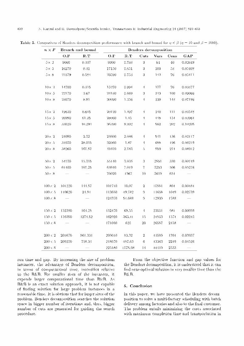
Table 3. Comparison of Benders decomposition performance with branch and bound for � < � (� = 10 and � = 1000).

n� F Branch and bound Benders decomposition

O.F R.T O.F R.T Cuts Vars Cons GAP

5� 2 9060 0.337 9300 0.788 3 64 40 0.02649

5� 5 16270 0.31 17150 0.651 3 103 58 0.05408

5� 8 22379 0.584 23590 0.753 3 142 76 0.05411

10� 2 14700 0.315 15270 0.994 4 177 76 0.03877

10� 5 22170 2.67 24180 0.669 3 243 100 0.09066

10� 8 28070 8.91 30090 1.256 4 339 148 0.07196

15� 2 19620 0.645 20120 1.497 4 340 111 0.02548

15� 5 26990 61.25 28060 1.45 4 448 154 0.03964

15� 8 33020 40.294 36390 9.992 4 562 202 0.10205

20� 2 24090 2.32 24600 2.086 4 541 136 0.02117

20� 5 31030 28.015 32960 1.87 4 688 196 0.06219

20� 8 38260 167.87 41670 2.783 5 859 274 0.08912

50� 2 54730 15.315 55140 3.035 3 2851 330 0.00749

50� 5 61400 107.25 64640 7.019 7 3253 506 0.05276

50� 8 { { 70020 1567 10 3619 654 {

100� 2 101220 144.87 101710 10.07 2 10881 804 0.00484

100� 5 110620 24.94 113650 49.782 9 11658 1049 0.02739

100� 8 { { 124370 54.688 9 12939 1788 {

150� 2 152380 164.28 152470 69.55 4 23551 981 0.00059

150� 5 159350 1274.52 162920 363.41 15 24853 1574 0.02240

150� 8 { { 171690 620 20 26587 2458 {

200� 2 201670 961.331 209610 83.32 2 41509 1394 0.03937

200� 5 209200 758.34 218670 487.63 6 43363 2249 0.04526

200� 8 { { 225180 1078.98 14 44419 2533 {

run time and gap. By increasing the size of probleminstances, the advantage of Benders decomposition,in terms of computational time, intensi�es relativeto the B&B. For smaller sizes of the instances, itexpends larger computational time than B&B. AsB&B is an exact solution approach, it is not capableof �nding solution for large problem instances in areasonable time. It is obvious that for larger sizes of theproblem, Benders decomposition searches the solutionspace in bigger number of iterations and, thus, biggernumber of cuts are generated for guiding the searchprocedure.

From the objective function and gap values forthe Benders decomposition, it is understood that it can�nd near-optimal solution in very smaller time than theB&B.

5. Conclusion

In this paper, we have presented the Benders decom-position to solve a multi-factory scheduling with batchdelivery among factories and also to the �nal customer.The problem entails minimizing the costs associatedwith maximum completion time and transportation in


Table 4. Comparison of Benders decomposition performance with branch and bound for � > � (� = 1000 and � = 10).

n� F Branch and bound Benders decompositionO.F R.T O.F R.T Cuts Vars Cons GAP

5� 2 590040 0.439 598050 1.157 4 70 46 0.013575� 5 1199050 0.483 1254050 0.757 3 103 58 0.045875� 8 1815050 0.721 1829050 1.034 6 190 113 0.00771

10� 2 935060 0.432 986070 1.799 6 183 83 0.0545510� 5 1523100 2.786 1672080 0.765 3 288 133 0.0978110� 8 2030100 7.907 2303090 1.099 4 339 148 0.13447

15� 2 1162080 1.48 1235120 1.932 5 334 107 0.0628515� 5 1758150 76.78 1878150 2.804 7 478 179 0.0682515� 8 2281150 303.21 2479140 15.79 15 706 315 0.08679

20� 2 1401110 1.791 1412200 2.76 6 541 138 0.0079120� 5 1992180 1317.36 2242190 2.47 5 838 307 0.1254920� 8 { { 2700200 14.07 9 931 329 {

50� 2 2972260 12.29 3040380 7.63 9 2851 336 0.0229150� 5 { { 3610500 498.89 80 3598 832 {750� 8 { { 4282480 3342 20 4147 1038 {

100� 2 5121510 1277.4 5148990 20.183 8 10701 660 0.00536100� 5 { { 6056000 169.18 20 12003 1379 {100� 8 { { 7006980 118.97 17 13299 2051 {

150� 2 { { 7758460 115.56 11 23551 988 {150� 5 { { 8495490 640.95 22 24688 1460 {150� 8 { 9488470 676.91 23 27499 3107 {

200� 2 { { 10199970 293.53 11 41401 1313 {200� 5 { { 11187920 1113.8 18 44338 2976 {200� 8 { 12038970 1624 27 45499 3311 {

the system and at the end of the system. The maincontribution of this paper is Benders reformulation ofthe problem, which facilitates the solution approachby decomposing the hard problem to two simpler prob-lems. The objective function of the master problem canalso be considered as the lower bound of the originalproblem.

Numerical experiments were conducted to eval-uate the e�ciency of the proposed method tacklinga large-scale real-world problem. The comparison ofthis method with the exact solution approach, adaptedB&B method, presented in [12] is performed. Theexperimental results con�rm the superior performance

of our presented method in terms of the run time tothe B&B algorithm, especially for a larger number ofproblem instances. It is clear that for larger sizes,the B&B cannot �nd the solution in reasonable time;but, Benders decomposition is capable of �nding near-optimal solution in the considered time.

For future research, we are seeking for ways toaccelerate the Benders decomposition algorithm, suchas developing a method to generate a set of cuts ateach iteration, for this problem. In addition, somemore research can be done with di�erent assumptionsof this problem, like unlimited number of vehicles,unlimited bu�ers, etc.


References

1. Moon, C., Seo, Y., Yun, Y. and Gen, M. \Adaptivegenetic algorithm for advanced planning in manufac-turing supply chain", J. Intell. Manuf., 17, pp. 509-522(2006).

2. Moon, C. and Seo, Y. \Evolutionary algorithm foradvanced process planning and scheduling in a multi-plant", Comput. Ind. Eng., 48, pp. 311-325 (2005).

3. Karatza, H.D. \Job scheduling in heterogeneous dis-tributed systems", Journal of Systems and Software,56(3), pp. 203-212 (2001).

4. Moon, C., Kim, J. and Hur, S. \Integrated processplanning and scheduling with minimizing total tar-diness in multi-plants supply chain", Computers &Industrial Engineering, 43(1-2), pp. 331-349 (2002).

5. Jia, H.Z., Nee, A.Y.C., Fuh, J.Y.H. and Zhang, Y.F.\A modi�ed genetic algorithm for distributed schedul-ing problems", Journal of Intelligent Manufacturing,14(3-4), pp. 351-362 (2003).

6. Chan, F.T.S., Chung, S.H. and Chan, P.L.Y. \Anadaptive genetic algorithm with dominated genes fordistributed scheduling problems", Expert Systems withApplications, 29(2), pp. 364-371 (2005).

7. Chan, F.T.S., Chung, S.H. and Chan, P.L.Y. \Appli-cation of genetic algorithms with dominant genes ina distributed scheduling problem in exible manufac-turing systems", International Journal of ProductionResearch, 44(3), pp. 523-543 (2006).

8. Chung, S.H., Lau, H.C.W., Choy, K.L., Ho, G.T.S.and Tse, Y.K. \Application of genetic approach foradvanced planning in multi-factory environment", In-ternational Journal of Production Economics, 127(2),pp. 300-308 (2010).

9. Sun, X.T., Chung, S.H. and Chan, F.T.S. \Integratedscheduling of a multi-product multi-factory manufac-turing system with maritime transport limits", Trans-portation Research Part E, 79, pp. 110-127 (2015).

10. H'Mida, F. and Lopez, P. \Multi-site scheduling underproduction and transportation constraints", Interna-tional Journal of Computer Integrated Manufacturing,26(3), pp. 252-266 (2013).

11. Huang, J.-Y. and Yao, M.-J. \On the optimal lot-sizing and scheduling problem in serial-type supplychain system using a time-varying lot-sizing policy",International Journal of Production Research, 51(3),pp. 735-750 (2013).

12. Karimi, N. and Davoudpour, H. \A branch andbound method for solving multi-factory supply chainscheduling with batch delivery", Expert Systems withApplications, 42, pp. 238-245 (2015).

13. Potts, C.N. \Technical notes analysis of a heuristic forone machine", Operation Research, 28(6), pp. 1436-1441 (1980).

14. Herrmann, J.W. and Lee, C.-Y. \On scheduling tominimize earliness-tardiness and batch delivery costswith a common due date", European Journal of Oper-ational Research, 70, pp. 272-288 (1993).

15. Cheng, T.C.E., Gordon, V.S. and Kovalyov, M.Y.\Single machine scheduling with batch deliveries",European Journal of Operational Research, 94(2), pp.277-283 (1996).

16. Hall, N.G. and Potts, C.N. \Supply chain scheduling:Batching and delivery", Operations Research, 51(4),pp. 566-584.

17. Mahdavi-Mazdeh, M., Shashaani, S., Ashouri, A. andHindi, K.S. \Single-machine batch scheduling minimiz-ing weighted ow times and delivery costs", AppliedMathematical Modelling, 35(1), pp. 563-570 (2011).

18. Mahdavi-Mazdeh, M., Sarhadi, M. and Hindi, K.S.\A branch-and-bound algorithm for single-machinescheduling with batch delivery minimizing ow timesand delivery costs", European Journal of OperationalResearch, 183, pp. 74-86 (2007).

19. Mahdavi-Mazdeh, M., Sarhadi, M. and Hindi, K.S.\A branch-and-bound algorithm for single-machinescheduling with batch delivery and job release times",Computers & Operations Research, 35, pp. 1099-1111(2008).

20. Rasti-barzoki, M. and Hejazi, S.R. \Minimizing theweighted number of tardy jobs with due date assign-ment and capacity-constrained deliveries for multiplecustomers in supply chains", European Journal ofOperational Research, 228(2), pp. 345-357 (2013).

21. Benders, J. \Partitioning procedures for solving mixedvariables programming problems", Numerische Math-ematik, 4, pp. 238-252 (1962).

22. Hooker, J.N. \Planning and scheduling to minimizetardiness", In Lecture Notes in Computer Science.Principles and Practice of Constraint Programming,3709, pp. 314-327 (2005).

23. Hooker, J.N. \An integrated method for planning andscheduling to minimize tardiness", Constraints, 11, pp.139-157 (2006).

24. Hooker, J.N. \Planning and scheduling by logic-basedbenders decomposition planning and scheduling bylogic-based benders decomposition", Operations Re-search, 55(3), 588-602 (2007).

25. Rinnooy Kan, A.H. G., Machine Scheduling Problems:Classi�cation, Complexity and Computations, Marti-nus Nijho�, The Hague, Neth (1976).

Biographies

Neda Karimi received her PhD degree in IndustrialEngineering in 2016. Her research is mainly focused onscheduling, supply chain, and mathematical modeling.

Hamid Davoudpour has been a Faculty Memberat Amikabir University, Tehran, Iran, since 1978.


He is currently Associate Professor in the Facultyof Industrial and Systems Engineering and Manage-ment.

His research interests include production planningand scheduling, and locations and allocation problems.

He is Chief Editor of International Journal of ModernScience and Technology. He has published 12 booksand more than 150 papers in international journals andpresented many others at national and internationalconferences.

a benders decomposition algorithm for multi-factory...

Documents