A Bialgebraic Approach to Automata and FormalLanguage Theory

James Worthington

Mathematics Department, Malott Hall, Cornell University, Ithaca, NY 14853-4201 USA

Abstract

A bialgebra is a structure which is simultaneously an algebra and a coalgebra,such that the algebraic and coalgebraic parts are compatible. Bialgebras areusually studied over a commutative ring. In this paper, we apply the definingdiagrams of algebras, coalgebras, and bialgebras to categories of semimodulesand semimodule homomorphisms over a commutative semiring. We then treatautomata as certain representation objects of algebras and formal languages aselements of dual algebras of coalgebras. Using this perspective, we demonstratemany analogies between the two theories. Finally, we show that there is anadjunction between the category of “algebraic” automata and the category ofdeterministic automata. Using this adjunction, we show that K-linear automa-ton morphisms can be used as the sole rule of inference in a complete proofsystem for automaton equivalence.

1. Introduction

Automata and formal languages are fundamental objects of study in theo-retical computer science. Classically, they have been studied from an algebraicperspective, focusing on transition matrices of automata, algebraic operationsdefined on formal power series, etc., as in the Kleene-Schutzenberger theorem.More recently, automata have been studied from a coalgebraic perspective, fo-cusing on the co-operations of transition and observation, and the coalgebraicnotion of bisimulation. See, for example, [15].

In this paper, we treat automata and formal languages from a bialgebraic per-spective: one that includes both algebraic and coalgebraic structures, with ap-propriate interactions between the two. This provides a rich framework to studyautomata and formal languages; using bialgebras, we can succinctly express op-erations on automata, operations on languages, maps between automata, lan-guage homomorphisms, and the interactions among them. We then show thatautomata as representation objects of algebras are related to the standard no-tion of a deterministic automaton via an adjunction.

Email address: worthing@math.cornell.edu (James Worthington)

Preprint submitted to Elsevier October 24, 2009

A note on terminology: there are two uses of the word “coalgebra” in theliterature we reference. In an algebra course, one would define “coalgebra” asa variety containing a counit map and the binary operations of addition andcomultiplication; i.e., the formal dual of an algebra (in the “vector space withmultiplication” sense). In computer science literature, the word “coalgebra”can refer to arbitrary F -coalgebras for a given endofunctor F of Set: so-called“universal coalgebra” [16]. Except for Section 9 below, our coalgebras are themore specific “algebra course” kind.

While bialgebras are usually studied over a commutative ring R, it is de-sirable to work over semirings when studying automata and formal languages.Hence we must define a tensor product for semimodules over a semiring; we showthat a tensor product with the correct universal property exists when the semir-ing in question is commutative. Semimodules over a semiring are in general notas well-behaved as vector spaces (neither are modules over a ring). However,free semimodules exist, and have all the useful properties that freeness entails.We remark that we treat input words as elements of free semimodules, and thatthe standard definition of a weighted automaton employs a free semimodule ona finite sets of states.

We then proceed by defining a bialgebra B on the set of all finite words overan alphabet Σ. The algebraic operation of multiplication describes how to “putwords together”; it is essentially concatenation. The coalgebraic operation ofcomultiplication, a map B → B⊗B, describes how to “split words apart”; thereare several comultiplications of interest.

Given an algebra A, we are interested in the structures on which A acts,i.e., its representation objects. We can encode an automaton as a representationobject of an algebra A equipped with a start state and an observation function.These automata compute elements of the dual module of A, which we view asformal languages. Automaton morphisms, i.e., linear maps between automatawhich preserve the language accepted, are shown to be instances of linear inter-twiners. Given a coalgebra C, the dual module of C also corresponds to a set oflanguages. A standard result is that a comultiplication on a coalgebra defines amultiplication on the dual module. For appropriate bialgebras, these two viewsof formal languages interact nicely, and we can use a bialgebra construction to“run two automata in parallel.”

Finally, we show that determinizing an automaton is essentially forgettingthe semimodule structure on its states. This idea is made precise with func-tors between categories of algebraic automata and categories of deterministicautomata. Each category has its own advantages: algebraic automata can becombined in useful ways, and can be nondeterministic, while deterministic au-tomata have unique minimizations. An adjunction between these two categoriesallows us to prove that a proof system for algebraic automata equivalence iscomplete; the rules of inference are automaton morphisms. This generalizesthe proof system treated explicitly in [18] and implicitly in [11] to arbitrarysemirings.

Other authors have explored the role of bialgebras in the theory of automataand formal languages. In [8] and [9], Grossman and Larson study the question of

2

which elements of the dual of a bialgebra can be represented by the action of thebialgebra on a finite object and prove the Myhill-Nerode theorem using notionsfrom the theory of algebras. Our definition of an automaton is a straightforwardgeneralization of theirs. In [4] and [5], Duchamp et al. examine rationality-preserving operations of languages defined using various comultiplications onthe algebra of input words, and construct the corresponding automata. Theyalso apply these ideas to problems in combinatorial physics.

This paper is organized as follows. In Section 2, we define algebras, coal-gebras, and bialgebras over a commutative ring R. In Section 3, we give thedefinitions of semirings and semimodules, and recall some useful facts and con-structions. Section 4 contains the construction of the tensor product of twosemimodules over a commutative semiring. Using this definition, in Section 5we apply the defining diagrams of algebras, coalgebras, and bialgebras to cat-egories of semimodules and semimodule homomorphisms. We treat automataas representation objects of algebras in Section 6, and then treat languages aselements of the dual algebra of a coalgebra in Section 7. In Section 8, we com-bine the algebraic and coalgebraic viewpoints, and show how to run automata inparallel if they are representation objects of a bialgebra. We give the adjunctionbetween deterministic automata and algebraic automata in Section 9, and theproof system in Section 10.

2. Algebras, Coalgebras, and Bialgebras

We now define algebras, coalgebras, and bialgebras over a commutative ringR. This material is completely standard; see [14] or [17] (note that Hopf algebrasand quantum groups are special cases of bialgebras).

2.1. AlgebrasDefinition 2.1. Let R be a commutative ring. An R-algebra (A, ·, η) is a ringA together with a ring homomorphism η : R → A such that η(R) is containedin the center of A and η(1R) = 1A.

Remark. The function η is called the unit map and defines an action of R onA via ra = η(r)a, so A is also an R-module.

To define an R-algebra diagrammatically, consider A as an R-module. Multipli-cation in A is an R-bilinear map A×A→ A, by distributivity and the fact thatη(R) is contained in the center of A. By the universal property of the tensorproduct, multiplication defines a unique R-linear map µ : A⊗A→ A (all tensorproducts in this section are over R). Associativity of multiplication implies that

3

the following diagram commutes:

A⊗A⊗Aµ⊗1A

xxqqqqqqqqqq1A⊗µ

&&MMMMMMMMMM

A⊗A

µ&&MMMMMMMMMMM A⊗A

µxxqqqqqqqqqqq

A.

The properties of the unit map can be expressed by the following commutativediagram (Recall that A⊗R ∼= A ∼= R⊗A):

A

1A

((η⊗1A

1A⊗η+3 A⊗A

µ // A.

Hence the diagrammatic definition of an R-algebra is an R-module A togetherwith R-module homomorphisms µ : A ⊗ A → A and η : R → A such that theabove diagrams commute.

Example 2.1. Let R be a commutative ring and P be the set of polynomialsover noncommuting variables x, y with coefficients in R. Addition and multipli-cation of polynomials make P into a ring. To make P into an R-algebra, defineη(r) to be the constant polynomial p(x, y) = r for r ∈ R.

Structure-preserving maps between algebras are called algebra maps.

Definition 2.2. LetA andB beR-algebras. An algebra map is anR-linear mapf : A→ B such that f(a1a2) = f(a1)f(a2) for all a1, a2 ∈ A, and f(1A) = 1B .Equivalently, an R-linear map f such that the following diagrams commute:

A⊗Af⊗f //

µA

B ⊗BµB

A

f // B

RηA

~~~~

~~~

ηB

AAA

AAAA

A

Af // B.

Given two R-algebras A and B, A⊗B becomes an R-algebra with multiplication

(a⊗ b) · (a′ ⊗ b′) = aa′ ⊗ bb′.

Diagrammatically, this multiplication can be expressed as a morphism

(A⊗B)⊗ (A⊗B)∼=

1A⊗σ⊗1B

// (A⊗A)⊗ (B ⊗B)µA⊗µB // A⊗B.

Here σ : A⊗B → B ⊗A; σ(a⊗ b) = (b⊗ a) is the usual transposition map.The unit of A⊗B is given by

R∼= // R⊗R

ηA⊗ηB // A⊗B.

4

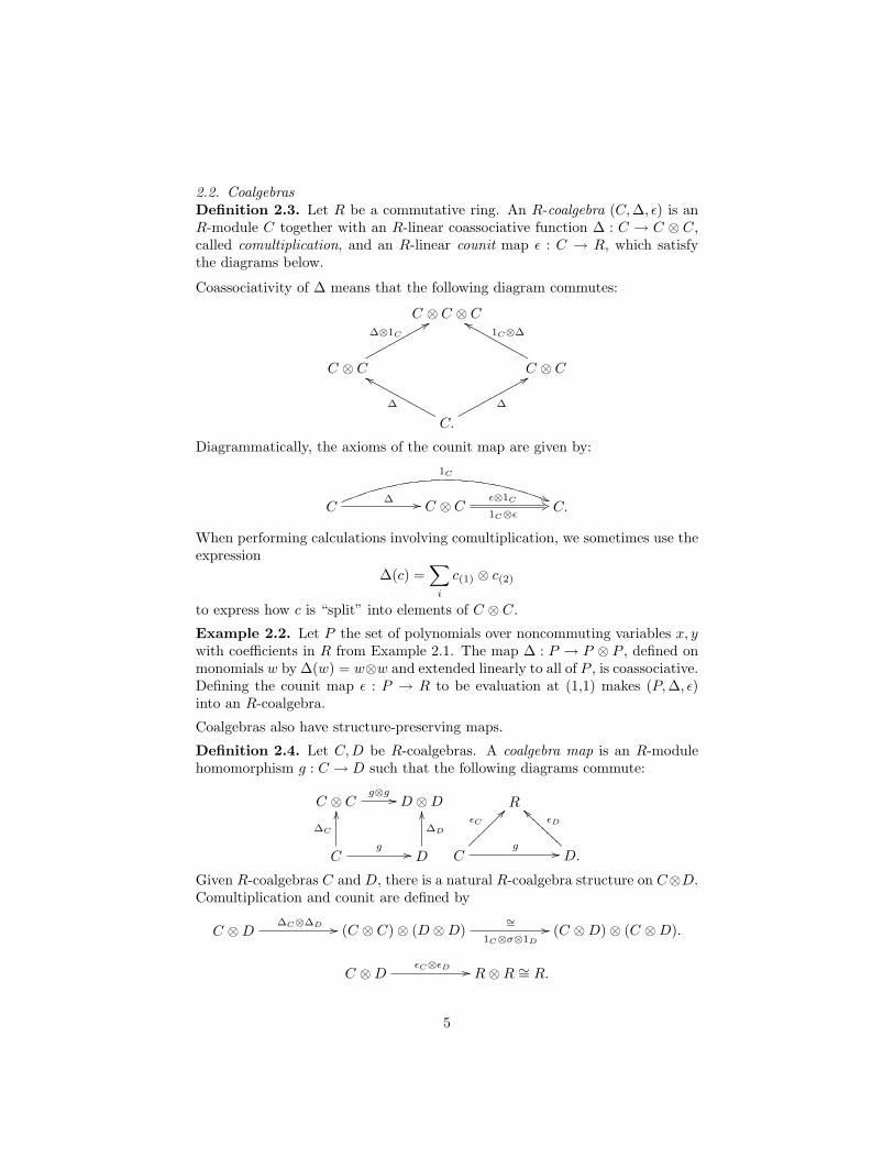
2.2. CoalgebrasDefinition 2.3. Let R be a commutative ring. An R-coalgebra (C,∆, ε) is anR-module C together with an R-linear coassociative function ∆ : C → C ⊗ C,called comultiplication, and an R-linear counit map ε : C → R, which satisfythe diagrams below.

Coassociativity of ∆ means that the following diagram commutes:

C ⊗ C ⊗ C

C ⊗ C

∆⊗1C

88qqqqqqqqqqC ⊗ C

1C⊗∆ffMMMMMMMMMM

C.

∆

ffMMMMMMMMMMM ∆

88qqqqqqqqqqq

Diagrammatically, the axioms of the counit map are given by:

C∆ //

1C

((C ⊗ C

ε⊗1C

1C⊗ε+3 C.

When performing calculations involving comultiplication, we sometimes use theexpression

∆(c) =∑i

c(1) ⊗ c(2)

to express how c is “split” into elements of C ⊗ C.

Example 2.2. Let P the set of polynomials over noncommuting variables x, ywith coefficients in R from Example 2.1. The map ∆ : P → P ⊗ P , defined onmonomials w by ∆(w) = w⊗w and extended linearly to all of P , is coassociative.Defining the counit map ε : P → R to be evaluation at (1,1) makes (P,∆, ε)into an R-coalgebra.

Coalgebras also have structure-preserving maps.

Definition 2.4. Let C,D be R-coalgebras. A coalgebra map is an R-modulehomomorphism g : C → D such that the following diagrams commute:

C ⊗ Cg⊗g // D ⊗D

Cg //

∆C

OO

D

∆D

OO R

Cg //

εC

??~~~~~~~D.

εD

``AAAAAAAA

Given R-coalgebras C and D, there is a natural R-coalgebra structure on C⊗D.Comultiplication and counit are defined by

C ⊗D∆C⊗∆D // (C ⊗ C)⊗ (D ⊗D)

∼=1C⊗σ⊗1D

// (C ⊗D)⊗ (C ⊗D).

C ⊗DεC⊗εD // R⊗R ∼= R.

5

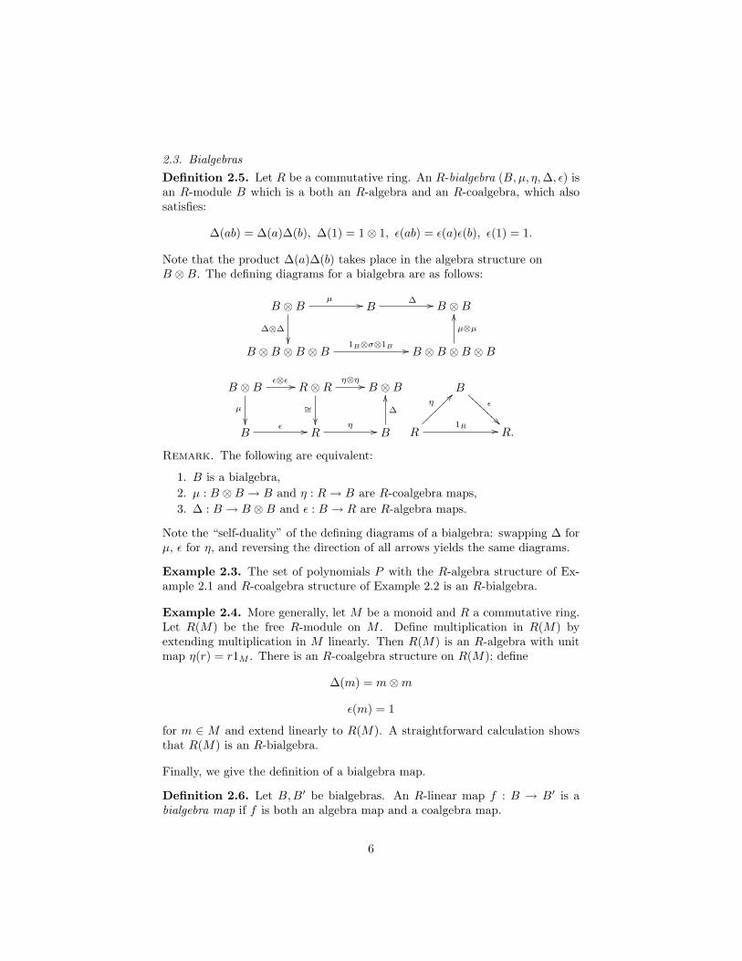
2.3. BialgebrasDefinition 2.5. Let R be a commutative ring. An R-bialgebra (B,µ, η,∆, ε) isan R-module B which is a both an R-algebra and an R-coalgebra, which alsosatisfies:

∆(ab) = ∆(a)∆(b), ∆(1) = 1⊗ 1, ε(ab) = ε(a)ε(b), ε(1) = 1.

Note that the product ∆(a)∆(b) takes place in the algebra structure onB ⊗B. The defining diagrams for a bialgebra are as follows:

B ⊗Bµ //

∆⊗∆

B∆ // B ⊗B

B ⊗B ⊗B ⊗B1B⊗σ⊗1B // B ⊗B ⊗B ⊗B

µ⊗µ

OO

B ⊗Bε⊗ε //

µ

R⊗Rη⊗η //

∼=

B ⊗B

Bε // R

η // B

∆

OO Bε

AAA

AAAA

A

R

η??~~~~~~~ 1R // R.

Remark. The following are equivalent:

1. B is a bialgebra,2. µ : B ⊗B → B and η : R→ B are R-coalgebra maps,3. ∆ : B → B ⊗B and ε : B → R are R-algebra maps.

Note the “self-duality” of the defining diagrams of a bialgebra: swapping ∆ forµ, ε for η, and reversing the direction of all arrows yields the same diagrams.

Example 2.3. The set of polynomials P with the R-algebra structure of Ex-ample 2.1 and R-coalgebra structure of Example 2.2 is an R-bialgebra.

Example 2.4. More generally, let M be a monoid and R a commutative ring.Let R(M) be the free R-module on M . Define multiplication in R(M) byextending multiplication in M linearly. Then R(M) is an R-algebra with unitmap η(r) = r1M . There is an R-coalgebra structure on R(M); define

∆(m) = m⊗m

ε(m) = 1

for m ∈ M and extend linearly to R(M). A straightforward calculation showsthat R(M) is an R-bialgebra.

Finally, we give the definition of a bialgebra map.

Definition 2.6. Let B,B′ be bialgebras. An R-linear map f : B → B′ is abialgebra map if f is both an algebra map and a coalgebra map.

6

3. Semirings and Semimodules

When studying automata and formal languages, it is natural to work oversemirings, which are “rings without subtraction”.

Definition 3.1. A semiring is a structure (K,+, ·, 0, 1) such that (K,+, 0) is acommutative monoid, (K, ·, 1) is a monoid, and the following laws hold:

j(k + l) = jk + jl

(k + l)j = kj + lj

0k = k0 = 0

for all j, k, l ∈ K. If (K, ·, 1) is a commutative monoid, then K is said to be acommutative semiring. If (K,+, 0) is an idempotent monoid, then K is said tobe an idempotent semiring.

The representation objects of semirings are known as semimodules.

Definition 3.2. Let K be a semiring. A left K-semimodule is a commutativemonoid (M,+, 0) along with a left action of K on M . The action satisfies thefollowing axioms:

(j + k)m = jm+ km

j(m+ n) = jm+ jn

(jk)m = j(km)

1Km = m

k0M = 0M = 0Km

for all j, k ∈ K and m,n ∈M . If addition in M is idempotent, M is said to bean idempotent left K-semimodule.

Right K-semimodules are defined analogously; in the sequel we give only “oneside” of a definition. If K is commutative, then every left K-semimodule canbe regarded as a right K-semimodule, and vice versa. In this case, we omit thewords “left” and “right”.

Example 3.1. Let K be a semiring and m,n be positive integers. The setof m × n matrices over K is a left K-semimodule, and the set of m ×m ma-trices over K is a semiring, using the standard definitions of matrix addition,multiplication, and left scalar multiplication.

Semimodules can be combined using the operations of direct sum and directproduct.

Definition 3.3. Let K be a semiring and Mi | i ∈ I be a collection of leftK-semimodules for some index set I. Let M be the cartesian product of theunderlying sets of the Mi’s. The direct product of the Mi’s, denoted

∏Mi, is the

set M endowed with pointwise addition and scalar multiplication. The directsum of the Mi’s, denoted

⊕Mi, is the subsemimodule of

∏Mi in which all but

finitely many of the coordinates are 0.

7

Remark. As usual, direct products and direct sums coincide when I is finite.

Homomorphisms, congruence relations, and factor semimodules are all definedstandardly.

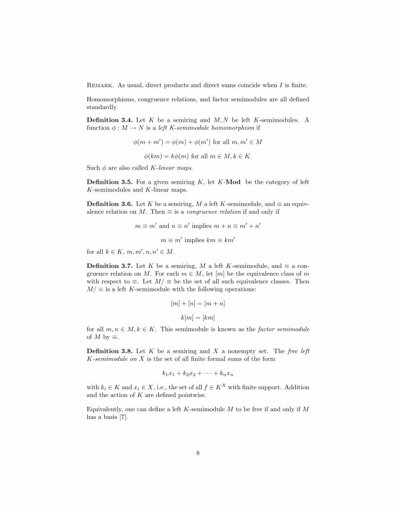
Definition 3.4. Let K be a semiring and M,N be left K-semimodules. Afunction φ : M → N is a left K-semimodule homomorphism if

φ(m+m′) = φ(m) + φ(m′) for all m,m′ ∈M

φ(km) = kφ(m) for all m ∈M,k ∈ K.

Such φ are also called K-linear maps.

Definition 3.5. For a given semiring K, let K-Mod be the category of leftK-semimodules and K-linear maps.

Definition 3.6. Let K be a semiring, M a left K-semimodule, and ≡ an equiv-alence relation on M . Then ≡ is a congruence relation if and only if

m ≡ m′ and n ≡ n′ implies m+ n ≡ m′ + n′

m ≡ m′ implies km ≡ km′

for all k ∈ K, m,m′, n, n′ ∈M .

Definition 3.7. Let K be a semiring, M a left K-semimodule, and ≡ a con-gruence relation on M . For each m ∈ M , let [m] be the equivalence class of mwith respect to ≡. Let M/ ≡ be the set of all such equivalence classes. ThenM/ ≡ is a left K-semimodule with the following operations:

[m] + [n] = [m+ n]

k[m] = [km]

for all m,n ∈ M,k ∈ K. This semimodule is known as the factor semimoduleof M by ≡.

Definition 3.8. Let K be a semiring and X a nonempty set. The free leftK-semimodule on X is the set of all finite formal sums of the form

k1x1 + k2x2 + · · ·+ knxn

with ki ∈ K and xi ∈ X, i.e., the set of all f ∈ KX with finite support. Additionand the action of K are defined pointwise.

Equivalently, one can define a left K-semimodule M to be free if and only if Mhas a basis [7].

8

Definition 3.9. Let M be a left K-semimodule and X a nonempty subset ofM . Then there is a K-linear map φ from the left K-semimodule of all functionsf ∈ KX with finite support to M given by

φ(f) =∑x∈X

f(x)x.

If φ is surjective, then X is said to be a set of generators of M . If φ is injective,then X is said to be linearly independent. If φ is a bijection, then X is said tobe a basis of M .

Remark. If M is a left K-semimodule with a basis of size m ∈ N, and N is aleft K-semimodule with a basis of size n ∈ N, then a K-linear map from M toN can be represented by an n×m matrix over K.

In the sequel, we use elementary facts about factor semimodules, free semimod-ules, congruence relations, and homomorphisms without comment. See [7] forproofs.

Definition 3.10. Let K be a commutative semiring and M a K-semimodule.The set of all K-linear maps M → K is denoted Hom(M,K).

Remark. In the sequel, the notation Hom(X,Y) always refers to the set of K-linear maps between X and Y , considered as K-semimodules, even if X and Yhave additional structure.

We end this section with two useful lemmas concerning dual semimodules. Theproofs are simple generalizations of the standard proofs for the case when K isa ring.

Lemma 3.1. Let K be a commutative semiring and M a K-semimodule. Theset Hom(M,K) can be endowed with a K-semimodule structure.

Proof. Hom(M,K) is a commutative monoid under pointwise addition. Letf ∈ Hom(M,K). The action of K on Hom(M,K), denoted ·, is defined byk · (f(m)) = kf(m). Commutativity of K is needed to show that the resultingfunctions are K-linear. Since f is K-linear, k · f(k′x) = k · k′f(x) = kk′f(x).In order for k · f to be K-linear, we must have k · f(k′x) = k′k · f(x) = k′kf(x).This means the equation kk′f(x) = k′kf(x) must hold, which is the case if Kis commutative.

Lemma 3.2. Let K be a commutative semiring, X be a finite nonempty set,and F the free K-semimodule on X. Then Hom(F,K) is also a free K-semimoduleon a set of size |X|.

Proof. Let x1, x2, . . . , xn be a basis of F and fi ∈ Hom(F,K) be such thatfi(xj) = 1 if i = j and 0 otherwise. We claim that the fi’s are a basis of

9

Hom(F,K). Let g ∈ Hom(F,K) and ai = g(xi). The fi’s form a generating setbecause

g(k1x1 + k2x2 + · · ·+ knxn) = k1g(x1) + k2g(x2) + · · ·+ kng(xn),

and so g = a1f1 +a2f2 + · · ·+anfn. Moreover, the fi’s are linearly independent;if

j1f1 + j2f2 + · · ·+ jnfn = j′1f1 + j′2f2 + · · ·+ j′nfn,

then evaluating each side on xi yields ji = j′i.

4. Tensor Products over Commutative Semirings

We wish to apply the defining diagrams of algebras, coalgebras, and bial-gebras to categories of K-semimodules and K-linear maps. To do this, weneed a notion of the tensor product of K-semimodules. Unfortunately, theliterature contains multiple inequivalent definitions of the tensor product of K-semimodules: the tensor product as defined in [7] is not the same as the tensorproduct defined in [13] or [10]. In fact, the tensor product defined in [7] is thetrivial K-semimodule when applied to idempotent K-semimodules.

We proceed by assuming that K is commutative and mimicking the con-struction of the tensor product of modules over a commutative ring in [12].This is essentially the construction used in [13] and [10]. The point is to work inthe appropriate category and construct an object with the appropriate universalproperty.

We recall the universal property of the tensor product over a commutativering R. Let M1,M2, ...,Mn be R-modules. Let C be the category whose objectsare n-multilinear maps

f : M1 ×M2 × · · · ×Mn → F

where F ranges over all R-modules. To define the morphisms of C, let

f : M1 ×M2 × · · · ×Mn → F and g : M1 ×M2 × · · · ×Mn → G

be objects of C. A morphism f → g is an R-linear map h : F → G such thathf = g. A tensor product of M1,M2, ...,Mn, denoted M1⊗RM2⊗R · · ·⊗RMn,is an initial object in this category. When it is clear from context, we omitthe subscript on the ⊗ symbol. By a standard argument, the tensor product isunique up to isomorphism.

We now construct the tensor product of semimodules over a commuta-tive semiring. Let K be a commutative semiring and M1,M2, ...,Mn be K-semimodules. Let T be the free K-semimodule on the (underlying) setM1 ×M2 × · · · ×Mn. Let ≡ be the congruence relation on T generated by theequivalences

(m1, ...,mi +Mim′i, ...,mn) ≡ (m1, ...,mi, ...,mn) +T (m1, ...,m

′i, ...,mn)

10

(m1, ..., kmi, ...,mn) ≡ k(m1, ...,mi, ...,mn)

for all k ∈ K,mi,m′i ∈Mi, 1 ≤ i ≤ n.

Let i : M1×M2×···×Mn → T be the canonical injection of M1×M2×···×Mn

into T . Let φ be the composition of i and the quotient map q : T → T/ ≡.

Lemma 4.1. The map φ is multilinear and is a tensor product ofM1,M2, ...,Mn.

Proof. Multilinearity of φ is obvious from its definition. Let G be a K-semimodule and

g : M1 ×M2 × · · · ×Mn → G

be a K-multilinear map. By freeness of T , there is an induced K-linear mapγ : T → G such that the following diagram commutes:

T

γ

M1 ×M2 × · · · ×Mn

i

66nnnnnnnnnnnnnn

g

((PPPPPPPPPPPPP

G.

The homomorphism γ defines a congruence relation, denoted ≡γ , on T via

t ≡γ t′ if and only if γ(t) = γ(t′)

for all t, t′ ∈ T . Since g is K-multilinear, we have ≡ ⊆ ≡γ , where ≡ is thecongruence relation used in the definition of the tensor product. Therefore γcan be factored through T/ ≡, and there is a K-linear map

g∗ : T/ ≡→ G

making the following diagram commute:

T/ ≡

g∗

M1 ×M2 × · · · ×Mn

φ

66mmmmmmmmmmmmm

g

((QQQQQQQQQQQQQQ

G.

The image of φ generates T/ ≡, so g∗ is uniquely determined.

For xi ∈Mi, we denote φ(x1, x2, ..., xn) by x1 ⊗ x2 ⊗ · · · ⊗ xn. Tensor productsenjoy many useful properties.

11

Lemma 4.2. Let K be a commutative semiring and N,M1,M2, ...,Mn be K-semimodules. Then:

1. There is a unique isomorphism

(M1 ⊗M2)⊗M3 →M1 ⊗ (M2 ⊗M3)

such that (m1 ⊗m2)⊗m3 7→ m1 ⊗ (m2 ⊗m3) for all mi ∈Mi.2. There is a unique isomorphism M1 ⊗M2 →M2 ⊗M1 such thatm1 ⊗m2 7→ m2 ⊗m1 for all mi ∈Mi.

3. K ⊗M1∼= M1

4. Let φ : M1 →M3 and ψ : M2 →M4 be K-linear maps. There is a uniqueK-linear map φ⊗ ψ : M1 ⊗M2 →M3 ⊗M4 such that(φ⊗ ψ)(m1 ⊗m3) = φ(m1)⊗ ψ(m2) for all m1 ∈M1,m2 ∈M2.

5. N ⊗⊕

i∈IMi∼=⊕

i∈I N ⊗Mi for any index set I.6. Let M ,N be free K-semimodules, with bases mii∈I and njj∈J , respec-

tively. Then M ⊗N is a free K-semimodule with basis mi ⊗ nj.

Proof. In [12], these properties are proven for tensor products over commuta-tive rings. The proofs rely on the universal property of the tensor product andare also valid in this case.

5. K-algebras, K-coalgebras, and K-bialgebras

Let K be a commutative semiring. We define K-algebras, K-coalgebras, K-bialgebras, and their respective maps by applying the relevant diagrams fromSection 2 to the category of K-semimodules and K-linear maps. To avoidclumsy terminology, we do not use the terms “semi-algebra”, “semi-coalgebra”,or “semi-bialgebra”.

Example 5.1. Let Σ = x, y be a set of noncommuting variables. Let P bethe set of polynomials over Σ with coefficients from the two-element idempotentsemiring K. Multiplication of polynomials is readily seen to be a K-bilinearfunction P × P → P , and therefore corresponds to a K-linear map P ⊗K P →P . Moreover, this map satisfies the associativity diagram. The underlying K-semimodule of P is the free K-semimodule on the set of all words w over x, y,so P ⊗ P is the free K-semimodule with basis w ⊗ w′ by Lemma 4.2.6. TheK-linear map η : K → P such that η(k) 7→ λxy.k satisfies the defining diagramof the unit map, and so P together with these maps forms a K-algebra.

The K-linear map ∆ defined on monomials as ∆(w) = w⊗w and extendedlinearly to all of P is easily seen to be coassociative. Defining ε(p(x, y)) = p(1, 1)makes P into a K-coalgebra. Furthermore, these maps satisfy the compatibilitycondition of a K-bialgebra, so P is a K-bialgebra.

We refer to constructions involving P as “the classical case” throughout thesequel.

12

Example 5.2. Given any set X and commutative semiring K, it follows fromgeneral considerations that there is a free K-algebra on X, which we denoteKX∗, and furthermore that there is an adjunction between the category ofK-algebras and K-algebra maps and Set.

One can associate two K-algebras to any K-semimodule M .

Lemma 5.1. Let M be a K-semimodule over a commutative semiring K. Theset of left endomorphisms of M , denoted Endl(M), is the set of all K-linearmaps M → M endowed with the following operations. Addition and scalarmultiplication are defined pointwise. Let f, g be K-linear maps M →M . Define

fg(a) = f(g(a)).

Similarly, let Endr(M) be the set of all K-linear maps M → M endowed withpointwise addition and scalar multiplication, and define multiplication by

(a)fg = ((a)f)g.

Then Endl(M) and Endr(M) are K-algebras.

Proof. Calculation.

Remark. The distinction between Endl(M) and Endr(M) allows us to defineautomata which read input words from right to left, and automata which readinput words from left to right.

6. K-algebras and Automata

In Example 5.1, we defined a K-algebra on the set of polynomials over thenoncommuting variables x, y. We can also think of elements of this algebraas finite sums of words over the alphabet x, y. In this section, we generalizethis idea and use the actions of K-algebras on K-semimodules to define transi-tions of automata, and list several analogs between algebraic constructions andconstructions on automata.

Definition 6.1. Let A be a K-algebra and M be a K-semimodule. A leftaction of A on M is a K-linear map A⊗M →M , denoted ., satisfying

(aa′) . m = a . (a′ . m)

1 . m = m

for all a, a′ ∈ A,m ∈M .

Right actions are defined analogously as K-linear maps / : M ⊗ A → M . Todefine an automaton, we also need a start state and an observation function.

Definition 6.2. A left K-linear automaton A = (M,A, s, .,Ω) consists of thefollowing:

13

1. A K-algebra A, a K-semimodule M , and a left action . of A on M ,2. An element s ∈M , called the start vector,3. A K-linear map Ω : M → K, called the observation function.

Remark. Equivalently, we could have defined a K-linear start function

α : K →M

and set s = α(1). This is useful in Section 9 below, but can add unnecessarysymbols to proofs. We use both variants, depending on the situation.

Automata are “pointed observable representation objects” of a K-algebra A.Right automata are defined similarly using a right action /. In the sequel, wegive only “one side” of a theorem or definition involving automata; the otherfollows mutatis mutandis. Intuitively, right automata read inputs from left toright, and left automata read inputs from right to left (see Example 6.2 below).

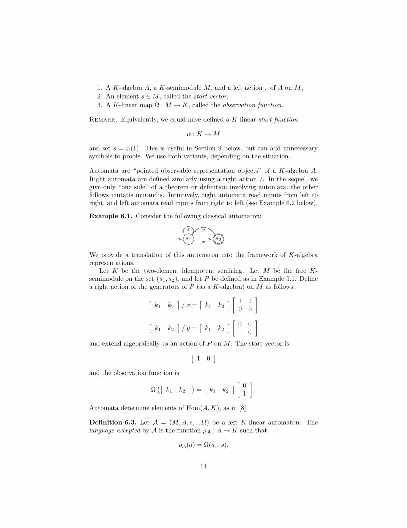
Example 6.1. Consider the following classical automaton:

// ?>=<89:;s1 x//

x ?>=<89:;76540123s2

y

We provide a translation of this automaton into the framework of K-algebrarepresentations.

Let K be the two-element idempotent semiring. Let M be the free K-semimodule on the set s1, s2, and let P be defined as in Example 5.1. Definea right action of the generators of P (as a K-algebra) on M as follows:

[k1 k2

]/ x =

[k1 k2

] [ 1 10 0

][k1 k2

]/ y =

[k1 k2

] [ 0 01 0

]and extend algebraically to an action of P on M . The start vector is[

1 0]

and the observation function is

Ω([

k1 k2

])=[k1 k2

] [ 01

].

Automata determine elements of Hom(A,K), as in [8].

Definition 6.3. Let A = (M,A, s, .,Ω) be a left K-linear automaton. Thelanguage accepted by A is the function ρA : A→ K such that

ρA(a) = Ω(a . s).

14

Lemma 6.1. The function ρA is an element of Hom(A,K).

Proof. Immediate since . and Ω are K-linear maps.

Definition 6.4. Let A and B be left K-linear automata. If ρA = ρB, then Aand B are said to be equivalent.

Functions between automata which preserve the language accepted are centralto the theory of automata; such functions have K-algebraic analogs.

Definition 6.5. Let A = (M,A, sA, .A,ΩA) and B = (N,A, sB, .B,ΩB) be leftK-linear automata. An K-linear automaton morphism from A to B is a mapφ : M → N such that

φ(sA) = sB (1)

φ(a .A m) = a .B φ(m) (2)

ΩA(m) = ΩB(φ(m)) (3)

for all m ∈M and a ∈ A.

Remark. Let V and W be R-modules. In the theory of R-algebras, an R-linearmap f : V →W which satisfies (2) is known as a linear intertwiner.

Remark. In the theory of automata, functions formally similar to automatonmorphisms have been called linear sequential morphisms [1], relational simu-lations [3], boolean bisimulations [6], and disimulations [18]. Disimulations arebased on the bisimulation lemma of Kleene algebra [11].

The following theorem, or a minor variant, is proven in most of the referencesmentioned in the above remark.

Theorem 6.1. Let A = (M,A, sA, .A,ΩA) and B = (N,A, sB, .B,ΩB) be leftK-linear automata, and let φ : A → B be a K-linear automaton morphism.Then A and B are equivalent.

Proof. For any a ∈ A,

ΩA(a .A sA) = ΩB(φ(a .A sA))= ΩB(a .B φ(sA))= ΩB(a .B sB).

A simple calculation proves the following lemma.

Lemma 6.2. Let A,B, C be left K-linear automata and φ : A → B, φ′ : B → Cbe automaton morphisms. Then φ′ φ : A → C is an automaton morphism.

Furthermore, for a left K-linear automaton A, the identity map of the under-lying K-semimodule of A is an automaton morphism. We therefore have thefollowing.

15

Lemma 6.3. For a given commutative semiring K, the collection of K-linearautomata and automaton morphisms forms a category.

Let A be a K-algebra. Elements of Hom(A,K) can be added and scaled byK, since Hom(A,K) is a K-semimodule by Lemma 3.1. Given automata Aand B, there is an automaton accepting ρA + ρB, and given k ∈ K, there is anautomaton accepting kρA.

Definition 6.6. Let A = (M,A, sA, .A,ΩA) and B = (N,A, sB, .B,ΩB) be leftK-linear automata. The direct sum of A and B is the left K-linear automatonA⊕ B = (M ⊕N,A, (sA, sB), .A⊕B,ΩA ⊕ ΩB), where

.A⊕B : A⊗ (M ⊕N)→M ⊕N,

.A⊕B(a⊗ (m,n)) = ((a .A m), (a .B n))

andΩA⊕B : M ⊕N → K,

ΩA⊕B(m,n) = ΩA(m) + ΩB(n).

The verification that .A⊕B is an action of A on M ⊕N is straightforward.

Theorem 6.2. Let A = (M,A, sA, .A,ΩA) and (N,A, sB, .B,ΩB) be left K-linear automata. Then ρA⊕B(a) = ρA(a) + ρB(a) for all a ∈ A.

Proof. For any a ∈ A,

ρA⊕B(a) = ΩA⊕B(a .A⊕B (sA, sB))= ΩA⊕B(a .A sA, a .B sB)= ΩA(a .A (sA)) + ΩB(a .B (sB))= ρA(a) + ρB(a).

Theorem 6.3. Let A = (M,A, s, .,Ω) be a left K-linear automaton, and letk ∈ K. Then kρA = ρA′ , where A′ = (M,A, ks, .,Ω).

Proof. For any a ∈ A, ρA′ = Ω(a . ks) = kΩ(a . s) = kρA by linearity.

Algebra maps can be used to translate the input of an automaton.

Definition 6.7. Let A,A′ be K-algebras and f : A → A′ a K-algebra map.Suppose A′ acts on a K-semimodule M . Then A also acts on M according tothe formula

a . m = f(a) . m

for a ∈ A,m ∈M. This is known as the pullback of the action of A′.

Automata theorists will recognize pullbacks as the main ingredient in the proofthat regular languages are closed under inverse homomorphisms.

Finally, we provide an example in which we reverse certain K-linear au-tomata using dual K-semimodules.

16

Example 6.2. Let A = (M,A, s, /,Ω) be a right K-linear automaton, and sup-pose that M is a free K-semimodule on a finite set X and A is the free K-algebraon a finite Σ. Then the left K-linear automaton B = (Hom(M,K), A,Ω, ., α∗),where

a . f(m) = f(m / a)

andα∗(m) = m · sT

satisfiesρA(w) = ρB(wR)

for all w ∈ Σ∗, where wR is the reverse of a word w. That A . Hom(M,K) isan action is an application of the standard fact that actions on (semi)modules“change sides” when the modules are dualized. See, for example, [2].

To prove the claim, let w = x1x2 · · ·xn with xi ∈ Σ. For some k ∈K, ρA(w) = k. Since M is a free K-module, the action of each x ∈ Σ on M isgiven by right multiplication by a |X|×|X| matrix Mx over K, and Ω(m) = m·vfor some |X| × 1 matrix v. By definition,

Ω(s . x1x2 · · ·xn) = s ·Mx1Mx2 · · ·Mxn · v = k.

Taking the transpose of both sides of this equation yields ρB(wR) = kT = k,with the slight abuse of notation vT = Ω. Note that the familiar transpose lawfrom linear algebra, (AB)T = BTAT, is valid for matrices over a commutativesemiring.

7. K-coalgebras and Formal Languages

Let C be a K-coalgebra. By Lemma 3.1, Hom(C,K) is a K-semimoduleunder the operations of pointwise addition and scalar multiplication. It is astandard fact that the coalgebra structure of C defines an algebra structure onHom(C,K).

Definition 7.1. Let (C,∆, ε) be a K-coalgebra and f, g ∈ Hom(C,K). Theconvolution product of f and g, denoted f ∗ g, is the element of Hom(C,K)defined by

f ∗ g = µK (f ⊗ g) ∆.

Here µK denotes multiplication in K.

Lemma 7.1. Let (C,∆, ε) be a K-coalgebra. There is a K-algebra structure onHom(C,K) with multiplication given by the convolution product and unit

η : K → C

η(k) = kε.

In particular, the multiplicative identity is ε.

17

Proof. The operation ∗ is associative because ∆ is coassociative:

f ∗ (g ∗ h) = µK(f ⊗ (µK(g ⊗ h))) ((1⊗∆) ∆)

(f ∗ g) ∗ h = µK((µK(f ⊗ g))⊗ h) ((∆⊗ 1) ∆)

and coassociativity of ∆ is exactly ((1 ⊗∆) ∆) = ((∆ ⊗ 1) ∆). The rest ofthe K-algebra requirements follow immediately from the definitions.

The relation between K-coalgebras and formal languages is as follows. Let Pbe as in Example 5.1. Note that an element of Hom(P,K) is completely deter-mined by its values on monomials, which we view as words over x, y. Thusthere is a one-to-one correspondence between subsets of x, y∗ and elements ofHom(P,K).

Consider the following comultiplications on P , defined on monomials andextended linearly:

∆1(w) = w ⊗ w

∆2(w) =∑

w1w2=w

w1 ⊗ w2.

Also consider the comultiplication defined as

∆3(x) = 1⊗ x+ x⊗ 1

∆3(y) = 1⊗ y + y ⊗ 1

extended as an algebra map to all of P . Moreover, we have two K-linear mapsgiven by:

ε1(p) = p(1, 1)

ε2(p) = p(0, 0)

for all p ∈ P . Then (P,∆1, ε1) is a K-coalgebra (cf. Example 2.2) as are(P,∆2, ε2) and (P,∆3, ε2).

A simple verification shows that the K-algebra on Hom(P,K) determined bythe K-coalgebra (P,∆1, ε1) corresponds to language intersection, with the mul-tiplicative identity corresponding to the language denoted by (x+ y)∗. The K-coalgebra (P,∆2, ε2) corresponds to language concatenation with identity λ,where λ is the empty word. Finally, the K-coalgebra (P,∆3, ε2) correspondsto the shuffle product of languages, again with identity λ (see [4] and also[14], Proposition 5.1.4). In each case, addition in the K-algebra on Hom(P,K)corresponds to the union of two languages.

We conclude this section with an example calculation. Let f ∈ Hom(P,K)correspond to the language denoted by x∗, and let g ∈ Hom(P,K) correspondto the language denoted by y∗. The following shows that yx ∈ f ∗ g, where the

18

comultiplication is ∆3:

µk f ⊗ g ∆3(xy) = µk f ⊗ g(1⊗ xy + y ⊗ x+ x⊗ y + xy ⊗ 1)= µK(f(1)⊗ g(xy) + f(y)⊗ g(x) + f(x)⊗ g(y) + f(xy)⊗ g(1))= µK(1⊗ 0 + 0⊗ 0 + 1⊗ 1 + 0⊗ 1)= 0 + 0 + 1 + 0= 1.

8. Automata, Languages, and K-bialgebras

A K-algebra A allows us to define automata which take elements of A asinput. These automata compute elements of Hom(A,K). Moreover, a K-coalgebra structure on A defines a multiplication on Hom(A,K). We now dis-cuss the relation between these products on Hom(A,K) and automata.

We first treat the case in which A is both a K-algebra and a K-coalgebra,without assuming that A is a K-bialgebra. Let A = (M,A, sA, .A,ΩA) andB = (N,A, sB, .B,ΩB) be K-linear automata. Applying the convolution productto ρA and ρB yields

ρA ∗ ρB(a) = µK (∑i

ρA(a(1) . sA)⊗ ρB(a(2) . sB)).

In words, the convolution product determines a formula with comultiplica-tion as a parameter. Different choices of comultiplication yield different productsof languages, as discussed in Section 7. When the languages are given by au-tomata, we can use this formula to obtain a succinct expression for the productof the two languages.

Of course, it would be even better if we could get an automaton acceptingthe product of the two languages. For a K-bialgebra, there is an easy way toconstruct such an automaton, which relies on a construction from the theory ofbialgebras.

We emphasize that a bialgebra structure is not necessary for an automatonaccepting ρA ∗ ρB to exist. Consider ∆2 and ∆3 as defined in Section 7. Theyagree on x and y, which generate P as an algebra, so at most one of them canbe an algebra map; ∆3 is an algebra map by definition. Therefore ∆2 is notpart of a bialgebra, and so we cannot use the construction to get an automatonaccepting the concatenation of two languages. Such an automaton exists, ofcourse, but it is not given by this construction.

Suppose B is a K-bialgebra. The first step is to define an action of B onM ⊗N from actions B .M M and B .N N (by an action of B on M , we meanan action of the underlying algebra of B on M).

Lemma 8.1. Let B be a K-bialgebra which acts on K-semimodules M and N .Then B acts on M ⊗N according to the diagram

B ⊗M ⊗N∆⊗1 // B ⊗B ⊗M ⊗N

1⊗σ⊗1// B ⊗M ⊗B ⊗N.M⊗.N// M ⊗N.

19

Proof. It is easy to see that the action of B on M ⊗N is a K-linear map suchthat 1 .m⊗ n = m⊗ n. To see that ab .m⊗ n = a . (b .m⊗ n), note that theequational definition of the action is

b .M⊗N (m⊗ n) =∑i

b(1) .M m⊗ b(2) .N n.

We have

ab . m⊗ n =∑i

ab(1) .M m⊗ ab(2) .N n

=∑i

a(1)b(1) .M m⊗ a(2)b(2) .N n

= a . (b . m⊗ n).

Definition 8.1. Let A = (M,B, sA, .A,ΩA) and B = (N,B, sB, .B,ΩB) beleft K-linear automata. The tensor product of A and B, denoted A⊗ B, is theautomaton (M ⊗N,B, sA ⊗ sB, .M⊗N ,ΩA ⊗ ΩB).

Remark. Note that since K ⊗K ∼= K, ΩM ⊗ ΩN : M ⊗N → K.

Theorem 8.1. Let A = (M,B, sA, .A,ΩA) and B = (N,B, sB, .B,ΩB) be leftK-linear automata. Then ρA⊗B = ρA ∗ ρB.

Proof. For any b ∈ B,

ρA⊗B(b) = ΩA⊗B(b .A⊗B (sA ⊗ sB))

= ΩA⊗B(∑i

b(1) .A sA ⊗ b(2) .B sB)

=∑i

ΩA(b(1) .A sA)ΩB(b(2) .B sB)

= ρA ∗ ρB(b).

In the classical case, this corresponds to “running two automata in parallel”.

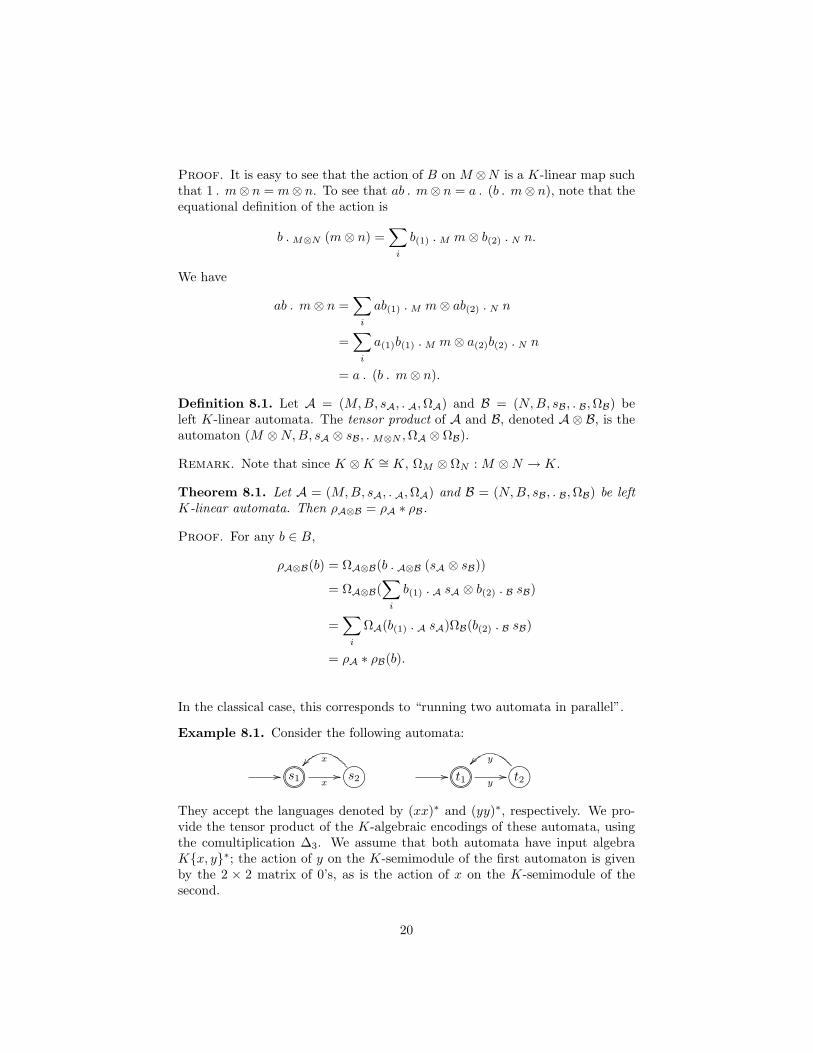
Example 8.1. Consider the following automata:

// ?>=<89:;76540123s1 x// ?>=<89:;s2

x// ?>=<89:;76540123t1 y

// ?>=<89:;t2y

They accept the languages denoted by (xx)∗ and (yy)∗, respectively. We pro-vide the tensor product of the K-algebraic encodings of these automata, usingthe comultiplication ∆3. We assume that both automata have input algebraKx, y∗; the action of y on the K-semimodule of the first automaton is givenby the 2 × 2 matrix of 0’s, as is the action of x on the K-semimodule of thesecond.

20

The K-semimodule of the tensor product is the free K-semimodule on theset s1 ⊗ t1, s1 ⊗ t2, s2 ⊗ t1, s2 ⊗ t2, by Lemma 4.2.6. The start vector is[

1 0 0 0],

the right x, y actions are given by0 0 1 00 0 0 11 0 0 00 1 0 0

,

0 1 0 01 0 0 00 0 0 10 0 1 0

respectively, and the observation function is given by

[k1 k2 k3 k4

]·

1000

.9. K-linear Automata and Deterministic Automata

We now define deterministic automata and relate deterministic automata toK-linear automata. We treat only right automata; the left automata case issimilar.

9.1. Deterministic AutomataLet the symbol 1 denote a canonical one-element set.

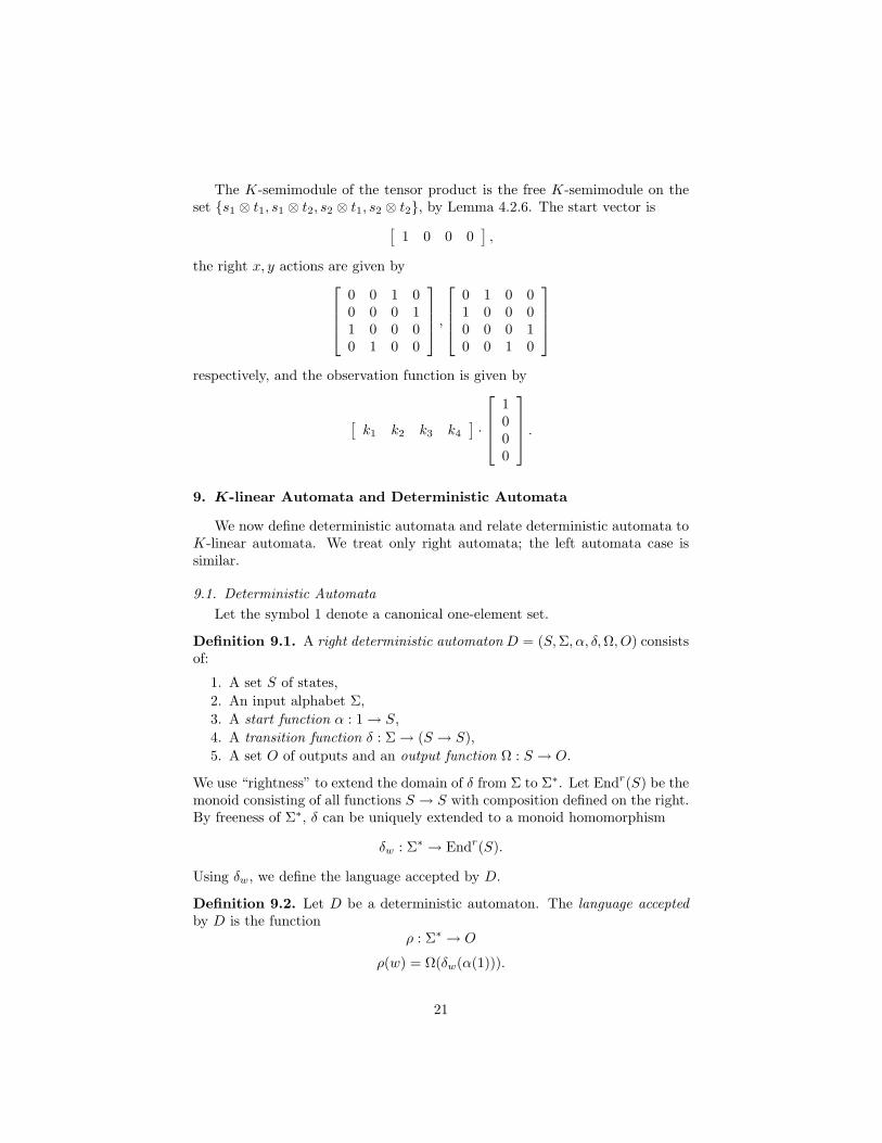
Definition 9.1. A right deterministic automaton D = (S,Σ, α, δ,Ω, O) consistsof:

1. A set S of states,2. An input alphabet Σ,3. A start function α : 1→ S,4. A transition function δ : Σ→ (S → S),5. A set O of outputs and an output function Ω : S → O.

We use “rightness” to extend the domain of δ from Σ to Σ∗. Let Endr(S) be themonoid consisting of all functions S → S with composition defined on the right.By freeness of Σ∗, δ can be uniquely extended to a monoid homomorphism

δw : Σ∗ → Endr(S).

Using δw, we define the language accepted by D.

Definition 9.2. Let D be a deterministic automaton. The language acceptedby D is the function

ρ : Σ∗ → O

ρ(w) = Ω(δw(α(1))).

21

Of special importance are maps between automata which preserve the languageaccepted.

Definition 9.3. Let D = (S,Σ, αD, δD,ΩD, O) and E = (T,Σ, αE , δE ,ΩE , O)be deterministic automata. A deterministic automaton morphism is a map

f : S → T

such that the following diagrams commute:

1αD //

αE >>>

>>>>

S

f

SδD //

f

S

f

SΩD //

f

O

T TδE

// T T.

ΩE

>>

If such a map exists, then ρD(w) = ρE(w) for all w ∈ Σ∗; the proof is es-sentially the same as the proof of Theorem 6.1. As with K-linear automata,deterministic automata and deterministic automaton morphisms form a cate-gory.

Given an automaton D, we can remove states that don’t contribute to ρD.

Definition 9.4. Let D = (S,Σ, α, δ,Ω, O) be a deterministic automaton. Astate s ∈ S is accessible if there exists a w ∈ Σ∗ such that

δw(α(1)) = s.

Definition 9.5. Let D = (S,Σ, α, δ,Ω, O) be a deterministic automaton. LetS′ be the set of accessible states of D and let i be the inclusion S′ → S. Theaccessible subautomaton of D is the automaton D′ = (S′,Σ, α, δ i,Ω i, O).

Lemma 9.1. Let D = (S,Σ, α, δ,Ω, O) be a deterministic automaton and letD′ be its accessible subautomaton. Then ρD = ρD′ .

Proof. The inclusion S′ → S is a deterministic automaton morphism.

A useful property of deterministic automata is that they can be minimized.This is a consequence of a certain category having a final object; we must firsttweak a definition.

Definition 9.6. A deterministic labelled transition system (dlts) D =(S,Σ, δ,Ω, O) is a deterministic automaton without a specified start state. Adeterministic labelled transition system morphism is defined as a deterministicautomaton morphism without the condition on the start state.

Definition 9.7. Let D = (S,Σ, δ,Ω, O) be a dlts, and let s ∈ S. The languageaccepted by s is the function

Ls(w) : Σ∗ → O

Ls(w) = Ω(δw(s)).

22

Theorem 9.1. Let Σ be an alphabet and O be a set of outputs. Let C be thecategory of dlts’s with input alphabet Σ and output set O, and morphisms thereof.Then F = (S,Σ, δ,Ω, O) is a final object of C, where

1. S = OΣ∗ ,2. δ(ψ)(w) = ψ(xw) for ψ ∈ OΣ∗ , x ∈ Σ, w ∈ Σ∗,3. Ω(ψ) = ψ(λ), for ψ ∈ OΣ∗ .

Proof. See Section 10 of [16] (also the references contained therein). Given adlts D, the unique morphism D → F is s 7→ Ls for s ∈ SD. In the classicalcase, F is the dlts with a state for each formal language L ⊆ Σ∗ and transitionsgiven by Brzozowski derivatives.

Definition 9.8. Let D = (S,Σ, α, δ,Ω, O) be a deterministic automaton withall states accessible. The minimization of D, denoted M(D), is the deterministicautomaton obtained by the following procedure:

1. Construct the underlying dlts D′ by ignoring the start function α.2. Map D′ to F via the unique morphism f : s 7→ L(s).3. M(D) = f(D′) endowed with start state f(αD(1)). The dlts morphism f

enriched with start state information is the unique deterministic automa-ton morphism D →M(D).

This definition is justified in [15]. The morphism D →M(D) is, in particular, afunction from the state set SD to the state set SM(D). Any D,D′ which acceptthe same language map to the same M(D) by definition, so |SM(D)| ≤ |SD|(this is true even if the automata involved have infinitely many states).

9.2. K-linear Automata to Deterministic AutomataLet A = (M,A,α, /,Ω) be a K-linear automaton. We wish to construct

a deterministic automaton D which is in some sense equivalent to A. This ispossible using the notion of an adjunction between categories. There are manyequivalent definitions of adjunctions used in practice, we recall the one mostuseful for our purposes.

Definition 9.9. Let A and D be categories, F a functor from D to A, and U afunctor from A to D. An adjunction from D to A is a bijection ψ which assignsto each arrow f : F (D)→ A of A an arrow ψf : D → U(A) of D such that

ψ(f Fh) = (ψf) h,

ψ(k f) = Uk (ψf)

holds for all f and all arrows h : D′ → D and k : A → A′. Equivalently, forevery arrow g : D → U(A),

ψ−1(gh) = ψ−1g (Fh),

ψ−1(Uk g) = k (ψ−1g)

(omitting unnecessary parentheses).

23

Example 9.1. Note that we use the notation of this example throughout thesequel. Let U ′ be the forgetful functor from K-Mod to Set and F ′ the corre-sponding free functor. The adjunction θ from Set to K-Mod takes as input aK-linear map φ : F ′(X) → M and returns the set map X → U ′(M) obtainedby restricting φ to X.

Our goal is to construct a “determinizing” functor from a category of K-linearautomata to a category of deterministic automata, and a “free K-linear” functorin the opposite direction, and then to show that these two functors are relatedby an adjunction. In order for this to work nicely, we make the following as-sumptions.

1. The input K-algebra of the K-linear automata is the free K-algebra on afinite set Σ.

2. The input alphabet of the deterministic automata is Σ, and the outputset of the deterministic automata is the underlying set of K.

When considering start functions, we treat K as F ′(1).Let A be a category of K-linear automata and K-linear automaton mor-

phisms, satisfying assumption 1 above, and let D be a category of deterministicautomata and deterministic automaton morphisms, satisfying assumption 2.We define a functor U from A to D which in the classical case corresponds todeterminization via the subset construction.

On K-linear automata, U behaves as follows. Given a K-linear automatonA = (M,KΣ∗, α, /,Ω),

U(A) = (U ′(M),Σ, θ(α), δ, U ′(Ω), U ′(K)),

where δ is defined as follows. The action M /KΣ∗ is equivalent to a K-algebramap

KΣ∗ → Endr(M).

Restricting this action to the generators of KΣ∗ yields a map t from Σ to theright endomorphism monoid of M ; define δ(x) = U ′(t(x)).

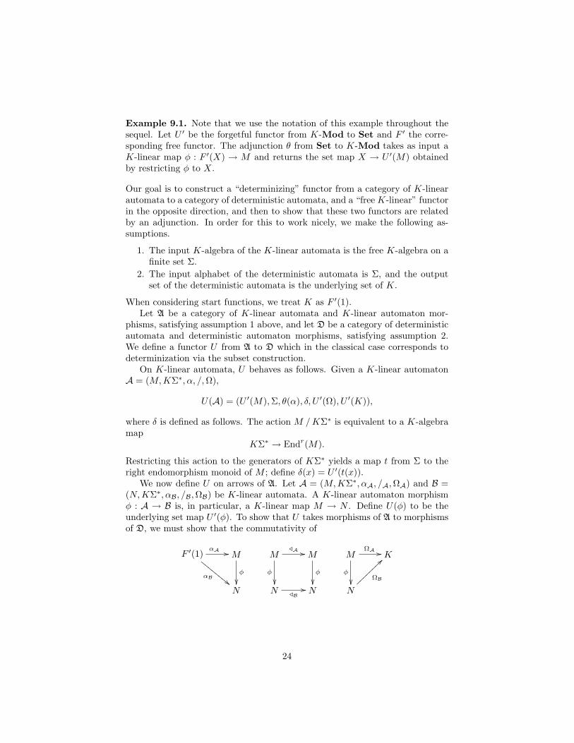
We now define U on arrows of A. Let A = (M,KΣ∗, αA, /A,ΩA) and B =(N,KΣ∗, αB, /B,ΩB) be K-linear automata. A K-linear automaton morphismφ : A → B is, in particular, a K-linear map M → N . Define U(φ) to be theunderlying set map U ′(φ). To show that U takes morphisms of A to morphismsof D, we must show that the commutativity of

F ′(1)αA //

αB""E

EEEE

EEE M

φ

M/A //

φ

M

φ

MΩA //

φ

K

N N /B// N N

ΩB

>>~~~~~~~~

24

implies the commutativity of

1θ(αA)//

θ(αB) !!DDD

DDDD

DD U ′(M)

U ′(φ)

U ′(M) δ //

U ′(φ)

U ′(M)

U ′(φ)

U ′(M)U ′(ΩA)//

U ′(φ)

U(K)

U ′(N) U ′(N)δ// U ′(N) U ′(N).

U ′(ΩB)

::uuuuuuuuu

The transition and output diagrams commute because the functor U ′ takes com-mutative diagrams to commutative diagrams. To show that the start functiondiagram commutes, note that

θ(φ αA) = U ′(φ) θ(αA)

since θ is an adjunction. Since αB = φ αA, we have θ(αB) = U ′(φ) θ(αA).

Theorem 9.2. The function U is a functor from A to D.

Proof. We have given the action of U on objects and morphisms of A. Itremains to show that

U(1A) = 1U(A),

U(φ′ φ) = U(φ′) U(φ).

This is the case because U is the restriction of the functor U ′ to K-linear mapswhich are also K-linear automaton morphisms.

The following theorem follows easily from the definitions.

Theorem 9.3. Let A be a K-linear automaton. Then θ(ρA) = ρU(A).

Remark. Depending on K, it is possible for U to take a K-linear automatonwhose underlying K-semimodule is the free K-semimodule on a finite set Xand return a deterministic automaton with infinitely many states. This is notsurprising; if the range of the language accepted by a deterministic automatonD is infinite, then D must have infinitely many states. Furthermore, even inthe classical case, it well-known that there are nondeterministic automata withn states such that any equivalent deterministic automaton requires a numberof states exponential in n. In other words, a K-semimodule structure can be asignificant asset to computation.

9.3. Deterministic Automata to K-linear AutomataWe now define a functor F : D → A. In the classical case, this functor is

used implicitly when encoding a deterministic automaton using matrices.Given a deterministic automaton D = (S,Σ, α, δ,Ω, U ′(K)), the free K-

linear automaton F (D) is

(F ′(S),KΣ∗, F ′(α), /, θ−1(Ω))

25

where / is defined as follows. Apply F ′ to δ(x) for each x ∈ Σ. This yields amap from Σ to Endr(F ′(S)), which has a unique extension to an algebra mapKΣ∗ → Endr(F ′(S)).

Let D = (S,Σ, αD, δD,ΩD, U ′(K)) and E = (T,Σ, αE , δE ,ΩE , U ′(K)) bedeterministic automata, and f a morphism D → E. Define F (f) = F ′(f);we must show that F ′(f) : F ′(S) → F ′(T ) is a K-linear automaton morphismF (D) → F (E). Dual to the determinizing case, it is easy to see that F ′(f)behaves well on the transition and input functions. We must show that

θ−1(ΩD) = θ−1(ΩE) F ′(f).

This follows from the equations θ−1(ΩE f) = θ−1(ΩE) F ′(f) andΩE f = ΩD.

Theorem 9.4. The function F defined above is a functor from D to A.

Proof. Similar to the proof of Theorem 9.2.

9.4. Adjunctions Between Categories of AutomataWe now show that the functors F and U defined above are related by an

adjunction. Let D = (S,Σ, αD, δ,ΩD, U ′(K)) be a deterministic automaton andA = (M,KΣ∗, αA, /,ΩA) a K-linear automaton. We must find a bijection

ψ : A(F (D), A)→ D(D,U(A))

such that the conditions of an adjunction are satisfied. We claim that the desiredφ is a restriction of the adjunction between K-Mod and Set.

Lemma 9.2. Let D = (S,Σ, αD, δ,ΩD, U ′(K)) be a deterministic automaton,A = (M,KΣ∗, αA, /,ΩA) a K-linear automaton, and φ a K-linear automatonmorphism F (D)→ A. Then

ψ(φ) = φ|S : D → U(A)

is a deterministic automaton morphism D → U(A).

Proof. By definition of F and U , and the fact that φ is a K-linear automatonmorphism, the following diagrams commute:

F ′(1)F ′(αD)//

αA$$H

HHHHHHHHF ′(S)

φ

F ′(S) δ //

φ

F ′(S)

φ

F ′(S)θ−1(ΩD) //

φ

K

M M /A// M M.

ΩA

77oooooooooooooo

To show that ψ(f) is a deterministic automaton morphism, we must show thethe commutativity of

1αD //

θ(αA) !!DDD

DDDD

DD S

ψ(φ)

SδD //

ψ(φ)

S

ψ(φ)

SΩD //

ψ(φ)

U ′(K)

U ′(M) U ′(M)δ// U ′(M) U ′(M).

U ′(ΩA)

::ttttttttt

26

This can easily be shown by diagram chasing.

Note that ψ(φ) = θ(φ), when φ is considered as a K-linear map.

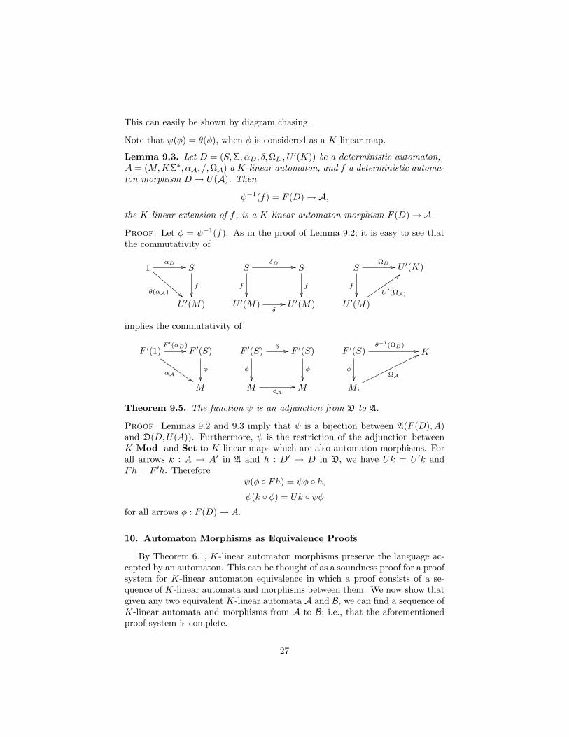
Lemma 9.3. Let D = (S,Σ, αD, δ,ΩD, U ′(K)) be a deterministic automaton,A = (M,KΣ∗, αA, /,ΩA) a K-linear automaton, and f a deterministic automa-ton morphism D → U(A). Then

ψ−1(f) = F (D)→ A,

the K-linear extension of f , is a K-linear automaton morphism F (D)→ A.

Proof. Let φ = ψ−1(f). As in the proof of Lemma 9.2; it is easy to see thatthe commutativity of

1αD //

θ(αA) !!DDD

DDDD

DD S

f

SδD //

f

S

f

SΩD //

f

U ′(K)

U ′(M) U ′(M)δ// U ′(M) U ′(M)

U ′(ΩA)

::uuuuuuuuu

implies the commutativity of

F ′(1)F ′(αD)//

αA$$H

HHHHHHHHF ′(S)

φ

F ′(S) δ //

φ

F ′(S)

φ

F ′(S)θ−1(ΩD) //

φ

K

M M /A// M M.

ΩA

77oooooooooooooo

Theorem 9.5. The function ψ is an adjunction from D to A.

Proof. Lemmas 9.2 and 9.3 imply that ψ is a bijection between A(F (D), A)and D(D,U(A)). Furthermore, ψ is the restriction of the adjunction betweenK-Mod and Set to K-linear maps which are also automaton morphisms. Forall arrows k : A → A′ in A and h : D′ → D in D, we have Uk = U ′k andFh = F ′h. Therefore

ψ(φ Fh) = ψφ h,ψ(k φ) = Uk ψφ

for all arrows φ : F (D)→ A.

10. Automaton Morphisms as Equivalence Proofs

By Theorem 6.1, K-linear automaton morphisms preserve the language ac-cepted by an automaton. This can be thought of as a soundness proof for a proofsystem for K-linear automaton equivalence in which a proof consists of a se-quence of K-linear automata and morphisms between them. We now show thatgiven any two equivalent K-linear automata A and B, we can find a sequence ofK-linear automata and morphisms from A to B; i.e., that the aforementionedproof system is complete.

27

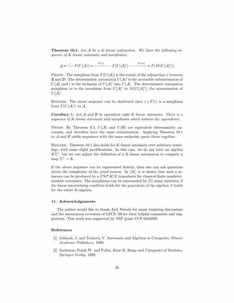
Theorem 10.1. Let A be a K-linear automaton. We have the following se-quence of K-linear automata and morphisms:

A F (U(A))εoo F (U(A)′)F (i)oo F (m) // F (M(U(A)′))

Proof. The morphism from F (U(A)) is the counit of the adjunction ψ betweenA and D. The deterministic automaton U(A)′ is the accessible subautomaton ofU(A) and i is the inclusion of U(A)′ into U(A). The deterministic automatonmorphism m is the morphism from U(A)′ to M(U(A)′), the minimization ofU(A)′.

Remark. The above sequence can be shortened since ε F (i) is a morphismfrom F (U(A)′) to A.

Corollary 1. Let A and B be equivalent right K-linear automata. There is asequence of K-linear automata and morphisms which witness the equivalence.

Proof. By Theorem 9.3, U(A) and U(B) are equivalent deterministic au-tomata, and therefore have the same minimization. Applying Theorem 10.1to A and B yields sequences with the same endpoint; paste them together.

Remark. Theorem 10.1 also holds for K-linear automata over arbitrary semir-ings, with some slight modifications. In this case, we do not have an algebraKΣ∗, but we can adjust the definition of a K-linear automaton to compute amap Σ∗ → K.

If the above sequence can be represented finitely, then one can ask questionsabout the complexity of the proof system. In [18], it is shown that such a se-quence can be produced by a PSPACE transducer for classical finite nondeter-ministic automata. The morphisms can be represented by |Σ| many matrices; ifthe linear intertwining condition holds for the generators of the algebra, it holdsfor the entire K-algebra.

11. Acknowledgements

The author would like to thank Anil Nerode for many inspiring discussionsand the anonymous reviewers of LFCS ’09 for their helpful comments and sug-gestions. This work was supported by NSF grant CCF-0635028.

References

[1] Adamek, J. and Trnkova, V. Automata and Algebras in Categories. KluwerAcademic Publishers. 1990.

[2] Anderson, Frank W. and Fuller, Kent R. Rings and Categories of Modules.Springer-Verlag. 1992.

28

[3] Buchholz, P. Bisimulation Relations for Weighted Automata. TheoreticalComputer Science, 393:109-123. 2008.

[4] Duchamp, G., Flouret, M., Laugerotte, E, and Luque, J.-G. Direct andDual Laws for Automata with Multiplicities. Theoretical Computer Science.267:105-120. 2001.

[5] Duchamp, G. and Tollu, Christophe. Sweedler’s Duals andSchutzenberger’s Calculus. Arxiv Preprint. arXiv:0712.0125v2.

[6] Fitting, Melvin. Bisimulations and Boolean Vectors. Advances in ModalLogic. Volume 4:97-125. 2003.

[7] Golan, Jonathan S. Semirings and Their Applications. Kluwer AcademicPublishers. 1999

[8] Grossman, R.L. and Larson, R.G. Bialgebras and Realizations. In HopfAlgebras: J. Bergen, S. Catoiu, and W. Chin, eds. pp 157-166. MarcelDekker, Inc. 2004.

[9] Grossman, R.L. and Larson, R.G. The Realization of Input-Output MapsUsing Bialgebras. Forum Mathematicum. Volume 4, pp. 109-121, 1992.

[10] Katsov, Yefim. Tensor Products and Injective Envelopes of Semimodulesover Additively Regular Semirings. Algebra Colloquium 4:2 121-131. 1997.

[11] Kozen, Dexter. A Completeness Theorem for Kleene Algebras and the Al-gebra of Regular Events. Infor. and Comput, 110(2):366-390. May 1994.

[12] Lang, Serge. Algebra: Revised Third Edition. Springer-Verlag. 2002.

[13] Litvinov, G.L., Masloc, V.P., and Shpiz, G.B. Tensor Products of Idem-potent Semimodules. An Algebraic Approach. Mathematical Notes. Vol 65,No. 4, 1999.

[14] Majid, Shahn. Foundations of Quantum Group Theory. Cambridge Uni-versity Press. 1995

[15] Rutten, J.J.M.M. Automata and Coinduction(An Exercise in Coalgebra).In Proc. CONCUR ’98, volume 1466 of LNCS, pages 194-218. Springer-Verlag, 1998.

[16] Rutten, J.J.M.M. Universal Coalgebra: A Theory of Systems. TheoreticalComputer Science. 249 pp. 3-80. 2000.

[17] Street, Ross. Quantum Groups: A Path to Current Algebra. CambridgeUniversity Press. 2007

[18] Worthington, James. Automatic Proof Generation in Kleene Algebra. In R.Berghammer, B. Moller, and G. Struth, editors, 10th Int. Conf. RelationalMethods in Computer Science (RelMiCS10) and 5th Int. Conf Applicationsof Kleene Algebra (AKA5), volume 4988 of LNCS, pages 382-396. Springer-Verlag, 2008.

29