a binomial lattice method for pricing corporate debt...
TRANSCRIPT

3/29/2007-624–JFQA #42:2 Broadie and Kaya Page 1
JOURNAL OF FINANCIAL AND QUANTITATIVE ANALYSIS Vol. 42, No. 2, June 2007, pp. 000–000COPYRIGHT 2007, SCHOOL OF BUSINESS ADMINISTRATION, UNIVERSITY OF WASHINGTON, SEATTLE, WA 98195
A Binomial Lattice Method for PricingCorporate Debt and Modeling Chapter 11Proceedings
Mark Broadie and Ozgur Kaya∗
Abstract
The pricing of corporate debt is still a challenging and active research area in corporatefinance. Starting with Merton (1974), many authors proposed a structural approach inwhich the value of the assets of the firm is modeled by a stochastic process, and all othervariables are derived from this basic process. These structural models have become morecomplex over time in order to capture more realistic aspects of bankruptcy proceedings.The literature in this area emphasizes closed-form solutions that are derived by either par-tial differential equation methods or analytical pricing techniques. However, it is not al-ways possible to build a comprehensive model with realistic model features and achieve aclosed-form solution at the same time. In this paper, we develop a binomial lattice methodthat can be used to handle complex structural models such as ones that include Chapter 11proceedings of the U.S. bankruptcy code. Although lattice methods have been widely usedin the option pricing literature, they are relatively new in corporate debt pricing. In partic-ular, the limited liability requirement of the equity holders needs to be handled carefully inthis context. Our method can be used to solve the Leland (1994) model and its extensionto the finite maturity case, the more complex model of Broadie, Chernov, and Sundaresan(2005), and others.
I. Introduction
A model for pricing risky corporate debt is important for both determiningoptimal capital structure and explaining observed yield spreads. In this paper,we are interested in the numerical evaluation of structural models of corporatedebt valuation. In a structural model, the value of the firm’s assets or the firm’searnings process is modeled as a primitive variable, and all other variables arederived from this basic variable. There is some freedom as to which aspects ofthe debt contracts to include in a model because these contracts are not uniform inpractice. Contractual agreements and bankruptcy laws may lead to different treat-ments when the firm fails to make debt payments and declares bankruptcy. For
∗Broadie, [email protected], Columbia University, Graduate School of Business, 3022 Broad-way, New York, NY 10027-6902; Kaya, [email protected], Columbia University, Department ofIndustrial Engineering and Operations Research, 500 West 120th St., New York, NY, 10027-6699.We thank Erwan Morellec (the referee) for many helpful comments and suggestions that improved thepaper. This work was supported in part by NSF grant DMS-0410234.
1

3/29/2007-624–JFQA #42:2 Broadie and Kaya Page 2
2 Journal of Financial and Quantitative Analysis
example, bankruptcy may lead to liquidation under Chapter 7 of the bankruptcycode, reorganization under Chapter 11, or the debt may be renegotiated privatelybetween debt holders and equity holders. The literature in this field is still growingas researchers add more complexity to the models in order to make their modelsmore realistic. Our aim in this paper is to introduce a numerical method thatcan be used to solve complex models when analytical pricing techniques are notavailable.
Merton (1974) first used a structural model for the valuation of risky zerocoupon bonds and risky perpetual coupon bonds. Black and Cox (1976) extendedthis work by considering the case when asset sales are not allowed and equitydilution is necessary to make coupon payments. Leland (1994) gives closed-form solutions for perpetual coupon bonds in a general setting that includes costlybankruptcy, tax benefits to coupon payments, and cash payouts by the firm. All ofthese models treat bankruptcy and liquidation as the same event: the firm is takenover by debt holders and liquidated when debt payments are not made in full.
More recent research attempts to model Chapter 11 proceedings by treat-ing bankruptcy and liquidation events separately. In Francois and Morellec (FMhereafter) (2004), after the firm value hits an endogenous barrier the equity hold-ers start servicing the debt strategically for the duration of a certain grace period.The firm is liquidated only if it stays in bankruptcy more than the granted graceperiod. The debt service while in bankruptcy is determined by a Nash bargaininggame. In other recent work, Broadie, Chernov, and Sundaresan (BCS hereafter)(2005) consider a similar setting, but they assume that instead of strategic debtservice while in bankruptcy, the coupon payments are stopped and are recordedin an arrears account. The earnings of the firm are collected in a separate account.The collected earnings are then used to pay the arrears when the firm comes outof bankruptcy. The firm is liquidated if it stays in bankruptcy for more than thegranted exclusivity period. Other models that treat bankruptcy and liquidationas separate events include Galai, Raviv, and Wiener (2003), Moraux (2002), andPaseka (2003).
Most of the existing models in the literature attempt to derive analytical val-uation formulas for debt and equity values by using simplifications to avoid timeand path dependence. To work in a time-independent setting, these models usu-ally price infinite maturity bonds although these bonds are almost never used inpractice. It is difficult to obtain analytical solutions in models of bankruptcy pro-ceedings that include automatic stay provisions, arrears payments, and grace pe-riods since these features introduce path dependency. Therefore, the events thathappen while the firm is in bankruptcy are simplified by introducing bargaininggames at the boundary or by complete debt forgiveness.
Recognizing that it is hard to build a model with realistic features and pre-serve analytical solutions at the same time, this paper introduces a numericalmethod that can help extend existing models or build more complex ones. Weuse lattice methods that are already very common in the option pricing literaturebut have rarely been used in corporate debt pricing. We model the evolution of thefirm’s assets on a discrete lattice and then use a backward solution procedure forthe valuation of all other securities. We show that the delicate issue of the limitedliability of equity holders can easily be handled using our method. Path depen-

3/29/2007-624–JFQA #42:2 Broadie and Kaya Page 3
Broadie and Kaya 3
dencies are also incorporated into our numerical method by increasing the statespace to record the value of path-dependent quantities. Our numerical method canbe used to extend models such as Leland (1994) and FM (2004) to finite maturitydebt, discrete coupon payments, or to solve new models such as BCS (2005).
Some other authors use numerical techniques in the context of corporatedebt pricing. Brennan and Schwartz (1978) solve the partial differential equation(PDE) for a firm that issues a bond paying discrete coupons. Their model is veryrestrictive with an exogenous bankruptcy boundary, and their valuation methoddoes not give debt and equity values separately. Anderson and Sundaresan (1996)use a binomial lattice method to price finite maturity bonds, but they do not allowequity dilution. They work in a simplified framework in which equity holdersand debt holders interact in an extensive form game to determine debt servicewhen firm cash flows are not enough to make the coupon payment. Anderson,Sundaresan, and Tychon (1996) show that it is possible to recast the Anderson-Sundaresan model in continuous time using PDEs. Anderson and Tu (1998) showhow to solve the related PDEs using finite difference methods. Fan and Sundare-san (2000) also use PDEs for valuation of finite maturity debt in a very similarsetting. However, all these models are models of renegotiation rather than reorga-nization in the sense of Chapter 11. Galai, Raviv, and Wiener (2003) consider amodel in which the firm’s excursions in the bankruptcy region can be given differ-ent weights based on severity and recentness. They assume there is an exogenousbankruptcy boundary and use Monte Carlo simulation for the valuation of zerocoupon bonds. However, it is not straightforward to use simulation methods toprice coupon bonds when equity dilution is allowed. The value of equity needs tobe known in order to decide if it is possible to make the coupon payment, and thisis not available when working forward in time.
As in some of the above-mentioned papers, it may be possible to write thePDEs for equity, debt, and firm values and to solve them using finite differencemethods. Although the resulting PDEs are usually simple and easy to solve nu-merically for plain vanilla models, they become much harder to solve once path-dependent variables such as grace period and arrears are introduced. It is not clearhow to treat these variables when discretizing the state space in a finite differencemethod. Our lattice method is much more intuitive and easier to implement forboth simple and complex models. By attaching auxiliary variables to lattice nodesbelow the bankruptcy boundary and by using interpolation techniques when nec-essary, these complexities are easily handled.
The rest of the paper is organized as follows. In Section II, we introducethe basic setup. In Sections III–V, we describe the implementation of our methodfor models with increasing complexity. We give some computational analysis inSection VI. Section VII concludes the paper.
II. Basic Setup
We denote the firm’s asset value as Vt and use it as the primitive variable, andhence all other variables can be seen as derivatives with respect to the asset value.We assume that the value of Vt is independent of the capital structure choices andits evolution under the risk-neutral measure Q is given by

3/29/2007-624–JFQA #42:2 Broadie and Kaya Page 4
4 Journal of Financial and Quantitative Analysis
dVt
Vt= (r − q)dt + σdWt,(1)
where Wt is a standard Brownian motion under Q, q is the payout ratio (i.e., cashflow) of the firm, and σ is the volatility of asset returns. We assume that the risk-free rate is constant at r, and that investors may lend and borrow freely at that rate.The process given above for the firm’s asset value uses the same representationas in the Black-Scholes model for a stock price that pays dividends at a constantrate q.
The instantaneous cash generated by the firm is denoted by δt and is givenby
δt = qVt.(2)
We assume that the firm issued a bond that promises to pay coupons at constanttotal rate C, continuously in time, until a default event occurs. The coupon is paidfrom the firm’s generated cash flow δt at time t and equity holders receive anysurplus δt − C in the form of dividends. There may be cases when C > δt, i.e.,the cash flows produced by the firm are not enough to make the coupon payment.For modeling purposes, we can treat (C − δt)+ as a negative cash flow for equityholders when C > δt. We will demonstrate that this is equivalent to dilution ofequity by the firm.
A. Binomial Lattice Method
We take Vt as our primitive variable, and using the representation in (1), builda lattice based on the binomial method of Cox, Ross, and Rubinstein (1979). It isstraightforward to adapt our method to other binomial, trinomial, and multinomiallattices. We start with an initial asset value V . Suppose that time horizon isdivided into small increments of length Δt. In the next time increment, the valueof the assets can increase by a factor of u to become Vu = uV , or decrease bya factor of d to become Vd = dV . The probability of an up move is p and theprobability of a down move is 1 − p. Choosing these parameters to match themean and variance of the continuous time process and imposing u = 1/d, weobtain
u = eσΔt,(3)
d = e−σΔt,
p =a − du − d
,
where
a = e(r−q)Δt.(4)
We want to compute the initial values of three quantities on the lattice. Thefirst of these is the claim of the equity holders after the debt is issued, which we

3/29/2007-624–JFQA #42:2 Broadie and Kaya Page 5
Broadie and Kaya 5
FIGURE 1
Binomial Step
Vu
Eu
Du
V Fu
E
D Vd
F Ed
Dd
Fd
1-p
p
denote by E. The second quantity is the claim of the debt holders, which wedenote by D. Finally, we want to compute the total firm value, which is denotedby F. A generic binomial step is shown in Figure 1.
At the current node, the present value of the equity is given by
E = e−rΔt (pEu + (1 − p)Ed) .(5)
The values of D and F can be calculated in a similar way:
D = e−rΔt (pDu + (1 − p)Dd) ,(6)
F = e−rΔt (pFu + (1 − p)Fd) .(7)
In computing (5)–(7), we are ignoring any events occuring at the current node.These values will be modified based on events such as coupon payments, liquida-tion, and distress cost. These model-specific modifications are considered in thesections that follow.
B. Equity Dilution and Limited Liability
In this section, we show how to incorporate the limited liability requirementin our numerical method. Basically, the limited liability requirement says thatshareholders should never experience negative cash flows and the most that theycan lose is their initial investment.
Suppose at a certain node in the binomial lattice we know the equity valuesin the next step, and these are given by Eu and Ed. Assume that at the currentnode, the firm has to make a coupon payment of C, and the cash flow generatedby the firm is given by δ. We want to know the value of equity, E, at the currentnode. The present value of equity ignoring the current coupon payment and thecurrent cash flow is given by
E = e−rΔt (pEu + (1 − p)Ed) .(8)
We denote the difference between the coupon payment and the current cash flowby C, i.e., we have C = C − δ. When the firm cash flow is less than the couponpayment, C is positive and it shows the amount that needs to be raised by equitydilution. A negative value of C should be interpreted as the excess firm cash flow

3/29/2007-624–JFQA #42:2 Broadie and Kaya Page 6
6 Journal of Financial and Quantitative Analysis
over the coupon payment that is to be received by equity holders. We show belowthat the equity value at the current node can be written as
E =
{0 if E ≤ C
E − C if E > C.(9)
This means that we do not need to go through tedious calculations of equity di-lution at each step even if the firm’s cash flow is not enough to cover the couponpayment. The equity value can be found by checking for the liquidation eventand treating the net coupon payment C as a negative cash flow to equity holdersif the firm is not liquidated. The following proposition shows that this is indeedequivalent to equity dilution.
Proposition 1. If the liquidation event is checked properly as in (9), treating netcoupon payments as negative cash flows to equity holders is equivalent to equitydilution, and this does not violate the limited liability requirement.
Proof. If C < 0, then the current firm cash flow is sufficient to cover the couponpayment, and the excess cash will be received by equity holders. Thus, E > C inthis case, and E = E − C will hold.
If C ≥ 0 and E ≤ C, then the equity holders have a liability that is largerthan their current value and, therefore, will choose to liquidate the firm. Thus,E = 0 in this case.
On the other hand if C ≥ 0, and E > C, then equity holders will still havepositive holdings after making the net coupon payment. Therefore, they willchoose to raise money by the dilution of equity and make the payment. With-out loss of generality, we can assume that there is one share outstanding. Equityholders will want to issue x more shares so that C is raised from the sale of newshares. After the equity dilution, there will be (1 + x) shares outstanding. Thenumber of new shares to be issued can be found by solving
x1 + x
E = C.(10)
The left side of equation (10) is the claim of the new shareholders in total equityvalue E after making the net coupon payment. Solving this equation gives thevalue of x as
x =C
E − C.(11)
The claim of the original shareholders in the equity value is 1/(1 + x). Wecan plug in the value of x from above to evaluate E:
E =1
1 + xE =
(1
1 + (C/(E − C ))
)E =
(E − C
E
)E = E − C.(12)
This can be generalized to all steps and nodes on the lattice by using induction.
We illustrate this further by a numerical example in Section III.B.

3/29/2007-624–JFQA #42:2 Broadie and Kaya Page 7
Broadie and Kaya 7
III. Bankruptcy with Immediate Liquidation
In this section, we consider the setting in which equity holders do not havethe option of going into default and postponing coupon payments. Either thecoupons are paid in full or the firm is liquidated in which case the debt holders re-ceive the proceedings from the liquidation process. Naturally, equity holders willchoose to liquidate the firm when the value of equity reaches zero. The limitedliability requirement prohibits states of the world in which equity has negativevalue. If the firm is liquidated, αVt is incurred as liquidation costs and debt hold-ers receive (1 − α)Vt.
We use the Leland (1994) model to illustrate our numerical method in thissetting. In this model, there is a consol bond with an infinite maturity that paysa constant coupon per unit time. An infinite maturity bond is convenient to workwith since this makes all the variables time independent. Leland writes the PDEssatisfied by the equity and debt values and solves them to obtain closed-formsolutions. However, his solutions do not extend to the case with finite maturitybonds because of time and path dependency. Using the binomial lattice method,we can easily extend Leland’s model to price finite maturity bonds.
A. Finite Maturity Case
Pricing the firm, debt, and equity on a binomial lattice is straightforwardonce the limited liability requirement is properly included. We assume that thefirm has just issued a bond with maturity T that pays a continuous coupon of Cper year, and has face value P. We assume that the effective tax rate is τ and allinterest payments are tax deductible. Because the tax benefits accrue at rate τCper year, the coupon payments effectively become (1 − τ)C per year from thefirm’s perspective. We choose a time step Δt and construct the binomial latticefor the unlevered asset value V as described in Section II.A. If the value of theassets at time t is Vt, then the instantaneous cash flow produced by the firm at t isgiven by δt = Vtq. On the binomial lattice, since we are using discrete time stepsthe total firm cash flow generated at a certain node with asset value Vt is given by(Vte qΔt−Vt). We will slightly abuse notation and use δt to denote this value, thuswe write
δt = VteqΔt − Vt.(13)
This representation accounts for the cash flows accumulated between timesteps. This also ensures that the binomial lattice matches the initial asset price V0
exactly.At maturity, we know the exact cash flows and the value of the firm’s assets,
so the debt, equity, and firm values are known. For all nodes at time T, we set

3/29/2007-624–JFQA #42:2 Broadie and Kaya Page 8
8 Journal of Financial and Quantitative Analysis
If VT + δT ≥ (1 − τ)CΔt + P : E = VT + δT − (1 − τ)CΔt − P,(14)
D = CΔt + P,
F = VT + δT + τCΔt.
If VT + δT < (1 − τ)CΔt + P : E = 0,
D = (1 − α)(VT + δT),F = (1 − α)(VT + δT).
Now we work backward to compute the equity, debt, and firm values at priortimes t < T. Since liquidation is determined by the value of the equity, we needto compute E first. We compute the present value of equity ignoring anything thathappens at the current node, which we denote by E,
E = e−rΔt (pEu + (1 − p)Ed) .(15)
If the sum of the firm cash flow, δt, and the present value of equity value, E,is enough to make the current coupon payment, there is no liquidation. However,if this sum is not enough to make the coupon payment, then liquidation occurs.So, we set:
If E + δt ≥ (1 − τ)CΔt : E = E + δt − (1 − τ)CΔt,(16)
D = CΔt + e−rΔt (pDu + (1 − p)Dd) ,
F = δt + e−rΔt (pFu + (1 − p)Fd) + τCΔt.
If E + δt < (1 − τ)CΔt : E = 0,
D = (1 − α)(Vt + δt),F = (1 − α)(Vt + δt).
Working backward until time zero, we can find the equity, debt, and firmvalues throughout the lattice. We illustrate this case with an example.
Example 1. We consider a firm with initial asset value V0 = 100, volatility σ =30%, and firm cash flow ratio of q = 4%. The risk-free rate is r = 6%. The firmhas just issued a bond with face value of P = 100, annual coupon payments ofC = 5, and with maturity T = 3 years. We assume that the liquidation cost and taxrate are zero, i.e., α = 0%, τ = 0%.
We want to find the equity, debt, and firm values. We use a three-step bino-mial lattice so that we have Δt = 1 year. We construct the binomial lattice for theasset value process Vt as described in Section II.A. We also record the firm cashflow δt as given in (13) and also the total payment due to debt holders at each step.This lattice is shown in Figure 2.
We then use (14)–(16) and work backward to find the equity, debt, and firmvalues at each step. Figure 3 shows these values. We find that E0 = 21.57, D0 =78.43, and F0 = 100.00.
B. Equivalent Equity Dilution Treatment
We return to the limited liability issue mentioned in Section II.B. The equityvalue E we found in Figure 3 can be decomposed into the cash flows on the paths

3/29/2007-624–JFQA #42:2 Broadie and Kaya Page 9
Broadie and Kaya 9
FIGURE 2
Binomial Lattice for Example 1
The top number at each node denotes the asset value, the middle number is the firm cash flow, and the bottom number isthe payment due to debt holders. Up and down probabilities are pu =0.4587 and pd =0.5413, respectively. The discountfactor is e−rΔt = 0.9418. The lattice construction using (3) and writing the firm cash flow using (13) matches the initialasset price exactly. For example, for the first time step we have: e−rΔt(pu(134.99+5.51)+pd(74.08+3.02))=100.00.Similar results hold for all time steps and nodes.
245.96
10.04
182.21 105.00
7.44
134.99 5.00 134.99
5.51 5.51
100.00 5.00 100.00 105.00
0.00 4.08
0.00 74.08 5.00 74.08
3.02 3.02
5.00 54.88 105.00
2.24
5.00 40.66
1.66
105.00
Time: 0 1 2 3
FIGURE 3
Equity, Debt, and Firm Value Computations for Example 1
The top number at each node denotes the equity value, the middle number is the debt value, and the bottom number isthe firm value.
151.00
105.00
85.76 256.00
103.89
44.91 189.65 35.49
95.59 105.00
21.57 140.49 14.42 140.49
78.43 89.67
100.00 4.25 104.08 0.00
72.85 77.11
77.11 0.00 77.11
57.12
57.12 0.00
42.32
42.32
Time: 0 1 2 3
of the binomial lattice. If we write explicitly the contribution of each path on thelattice to the value of E, we obtain the values shown in Table 1. The probabilityof following each path is also shown in the last column of the table. Multiplyingthe discounted cash flows with the probabilities and summing up, we can obtainthe same equity value that we find from the lattice, which is E = 21.57. We seefrom the table that the discounted cash flows on paths 4, 6, 7, and 8 are negative.This seems counterintuitive and in violation of the limited liability requirement.However, we show below that this is just a computational convenience and weobtain the same result when we use explicit dilution of equity.
The path cash flows can be decomposed in a different way when we lookat the situation from the equity dilution point of view. We will need to calculate

3/29/2007-624–JFQA #42:2 Broadie and Kaya Page 10
10 Journal of Financial and Quantitative Analysis
TABLE 1
Equity Cash Flow Decomposition
The letter u denotes an up move in the lattice and d denotes a down move. Corresponding probabilities are pu = 0.4587and pd = 0.5413. The discount factor is e−rΔt = 0.9418.
Cash FlowsPath Path Discounted PathNo. Direction 1 2 3 Payoff Prob.
1 u–u–u 0.51 2.44 151.00 128.76 0.09652 u–u–d 0.51 2.44 35.49 32.29 0.11393 u–d–u 0.51 −0.92 35.49 29.31 0.11394 u–d–d 0.51 −0.92 0.00 −0.34 0.13445 d–u–u −1.98 −0.92 35.49 26.97 0.11396 d–u–d −1.98 −0.92 0.00 −2.68 0.13447 d–d–u −1.98 0.00 0.00 −1.86 0.13448 d–d–d −1.98 0.00 0.00 −1.86 0.1586
the dilution proportion (1 + x) where x is as given in (11) for each node, and usethis to calculate the total number of shares outstanding. Once we do this, we canassume that the equity holders are exposed only to positive cash flows since thenegative cash flows are handled by equity dilution. Therefore, we compute thecash flows (δt − C)+ for the intermediate nodes and (V + δt − C − P)+ for theterminal nodes. The lattice in Figure 4 shows these calculations. The top numberis the net cash flow to be shared by total equity holders, and the bottom numberis the equity dilution proportion. The dilution proportion at a node is set to zeroif the firm has been liquidated.
FIGURE 4
Equity Dilution Calculations for Example 1
The top number at each node shows positive cash flows to equity holders, and the bottom number shows the equitydilution ratios.
151.00
1.00
2.44
1.00
0.51 35.49
1.00 1.00
0.00 0.00
1.00 1.06
0.00 0.00
1.46 0.00
0.00
0.00
0.00
0.00
Time: 0 1 2 3
We again write each path separately and look at the contribution of each path.The shares are diluted along the way to make the coupon payments. Therefore,if there are N shares outstanding at a particular node, the original shareholderswill have a claim of 1/N in the cash flow occurring at that node. N is foundby multiplying the dilution proportions of the nodes along each path. Table 2shows these values explicitly. We obtain the net discounted contribution fromeach path by discounting all the cash flows back to time zero and adding them up.

3/29/2007-624–JFQA #42:2 Broadie and Kaya Page 11
Broadie and Kaya 11
Multiplying the contribution of each path with path probability and summing up,we find the equity value as E = 21.57.
TABLE 2
Equity Dilution Path Decomposition
The numbers below cash flows show the total number of outstanding shares. If this number is zero, it means the firm hasbeen liquidated.
Cash FlowsPath Path Discounted PathNo. Direction 1 2 3 Payoff Prob.
1 u–u–u 0.51 2.44 151.00 128.76 0.0965(1.00) (1.00) (1.00)
2 u–u–d 0.51 2.44 35.49 32.29 0.1139(1.00) (1.00) (1.00)
3 u–d–u 0.51 0.00 35.49 28.35 0.1139(1.00) (1.06) (1.06)
4 u–d–d 0.51 0.00 0.00 0.48 0.1344(1.00) (1.06) (0.00)
5 d–u–u 0.00 0.00 35.49 19.02 0.1139(1.46) (1.56) (1.56)
6 d–u–d 0.00 0.00 0.00 0.00 0.1344(1.46) (1.56) (0.00)
7 d–d–u 0.00 0.00 0.00 0.00 0.1344(1.46) (0.00) (0.00)
8 d–d–d 0.00 0.00 0.00 0.00 0.1586(1.46) (0.00) (0.00)
The equity dilution approach demonstrated in Table 2 and the cash flow ap-proach demonstrated in Table 1 give exactly the same results. This is a numericalillustration of Proposition 1. This result is very useful because the cash flow ap-proach is computationally much easier to apply on a binomial lattice.
C. Infinite Maturity Case
The procedure described above can also be used to price a consol bond withinfinite maturity. We need to use a very long time horizon, such as T = 200 years,and change the terminal condition in (14). The terminal condition is not veryimportant since the time horizon is very long and the effect of the terminal nodeson initial prices is very small. If the bond were riskless, its price would be C/r.So, we treat the bond as if it has face value C/r and maturity T. At the final nodes,we set:
If VT >Cr
: E = VT − Cr
,(17)
D =Cr
,
F = VT .
If VT <Cr
: E = 0,
D = (1 − α)VT ,
F = (1 − α)VT .

3/29/2007-624–JFQA #42:2 Broadie and Kaya Page 12
12 Journal of Financial and Quantitative Analysis
We then work backward and use (16) to update the values at the nodes other thanthe terminal node.
Leland (1994) solves for the liquidation boundary, that is, the value of Vthat gives zero equity value using PDE methods and invoking the smooth pastingcondition. The above procedure achieves this boundary endogenously. In theconsol bond setting, the liquidation boundary is constant and time independent.As we work backward in the lattice, we observe zero equity value below a certainlevel of nodes. The recursive procedure given in (16) computes the equity valueby comparing continuation and stopping values as seen from the perspective ofequity holders. Thus, the usual smooth pasting condition will be obtained inthe limit as Δt goes to zero. See Dixit and Pindick ((1994), pp. 130–132) for adiscussion of the optimal stopping problem and the smooth pasting condition.
D. Convergence of the Method
Leland (1994) gives closed-form solutions for the infinite maturity bond inthe setting described in the previous sections. We include these formulas in theAppendix for reference. In this section, we analyze the convergence rate andbehavior of our numerical method by comparing our numerical results with ana-lytical results.
The pricing of equity is similar to the pricing of a call option. Because of thelimited liability principle, when equity holders’ net worth is less than the couponpayment due, they will default on the debt obligation, and hand the firm over to thedebt holders. Thus, there will be an implicit default boundary on the lattice belowwhich the equity has value zero. The pricing of debt is similar to the pricing ofa barrier option. When equity holders default on their debt, the firm is liquidatedand debt holders receive what is left of the firm. So the default boundary acts as aknockout barrier on which debt value achieves its liquidation value.
Figure 5 shows the convergence of debt and equity pricing errors as the num-ber of time steps is increased. Here the pricing error is defined as the differencebetween the formula value and the value from the lattice. As the number of timesteps is increased, the spacing of the nodes on the lattice becomes finer. We useT =200 as the maturity of the bond on the lattice to approximate an infinite matu-rity bond. We find that increasing this maturity further does not have a significanteffect on the prices produced by the lattice. Figure 6 shows a magnified versionof the same convergence graph.
We see that the convergence of the equity error is smooth while debt errorconvergence exhibits an oscillation similar to the ones observed in the pricing ofa barrier option (see, for example, Boyle and Lau (1994)). There are two sourcesof error on the lattice. One is the discretization error caused by approximating thecontinuous processes by their discretized versions on the lattice. The other is thebarrier error caused by approximating the values of the quantities on the defaultboundary. The value of equity is already close to zero near the default boundary,therefore, its value is not affected significantly by the barrier error. However, debtis sensitive to both the value and the location of the boundary since its value isaffected by the liquidation event. The barrier error can further be decomposed intotwo components. One source of error comes from the uncertainty of the exact

3/29/2007-624–JFQA #42:2 Broadie and Kaya Page 13
Broadie and Kaya 13
FIGURE 5
Convergence of Debt and Equity Errors for the Leland (1994) Model
Model parameters are V0 = 100, σ = 20%, C = 3.0, r = 5%, q = 4%, α = 50%, and τ = 0%. The true value of debt is49.8527, and the true value of equity is 46.0567.
-0.3
-0.2
-0.1
0
0.1
0.2
0.3
0.4
0.5
0.6
0 40,000 80,000 120,000 160,000 200,000
Steps
Err
or
Debt ErrorEquity Error
FIGURE 6
A Magnified View of the Convergence Graph in Figure 5
Figure 6 shows the oscillating pattern in the convergence of the debt value.
-0.4
-0.3
-0.2
-0.1
0
0.1
0.2
0.3
0.4
5,000 6,000 7,000 8,000 9,000 10,000
Steps
Err
or
Debt ErrorEquity Error
default boundary. The default boundary is also approximated on the lattice bylooking at the first point on which equity fails to make the coupon payment. Thismay differ slightly from the true bankruptcy point because of the discretizationerror. The second component of barrier error comes from the relative positioningof the barrier between the nodes. On a lattice, even if the barrier is betweenthe lattice nodes, it will effectively be moved to coincide with a level of nodessince the calculations are done on the nodes of the lattice only. These two effectscontribute to the debt error and cause the oscillatory behavior of the debt values.
We can estimate the convergence rate of the debt and equity errors by posit-ing a functional form in which |error| ≈ Mβ , i.e., absolute value of the error is
3/29/2007-624–JFQA #42:2 Broadie and Kaya Page 14
14 Journal of Financial and Quantitative Analysis
proportional to M, the number of time steps on the lattice. We can estimate β byusing the error values from the convergence graph in Figure 6. For equity error,we obtain a β value of −1.00, which indicates that the equity error converges lin-early as the number of time steps is increased. For debt error, we use the valueson the tips of the zigzag patterns for estimation and obtain a β value of −0.58.Gobet (1999) shows that the convergence rate for a barrier option is o(M− 1
2 ). Ac-cording to our numerical results, the convergence rate of debt error is indeed closeto square root convergence similar to a barrier option.
Interpolation methods such as the one given in Derman, Kani, Ergener, andBardhan (1995) may help in reducing the size of the oscillations in the debt value.Even without any numerical improvements, the highest debt error when usingaround 5,000 time steps is less than 0.5% of the debt value. This level of accu-racy is sufficient for corporate debt pricing where one is interested in qualitativecomparisons with different parameter values.
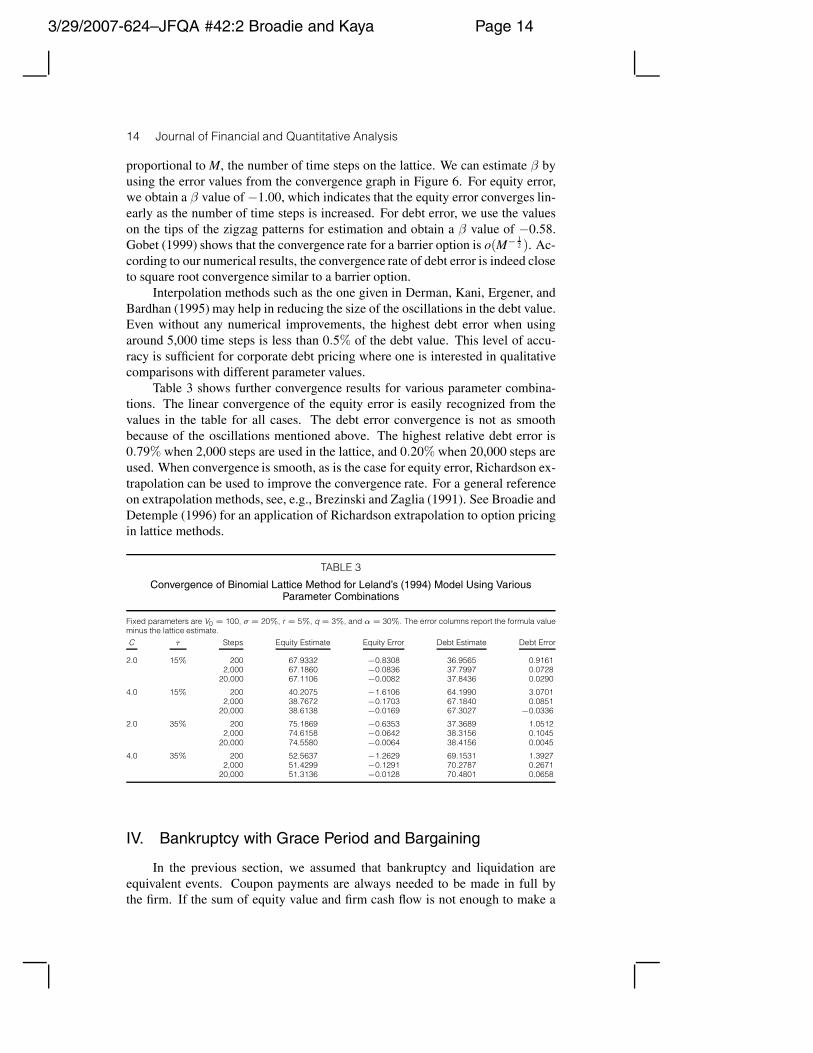
Table 3 shows further convergence results for various parameter combina-tions. The linear convergence of the equity error is easily recognized from thevalues in the table for all cases. The debt error convergence is not as smoothbecause of the oscillations mentioned above. The highest relative debt error is0.79% when 2,000 steps are used in the lattice, and 0.20% when 20,000 steps areused. When convergence is smooth, as is the case for equity error, Richardson ex-trapolation can be used to improve the convergence rate. For a general referenceon extrapolation methods, see, e.g., Brezinski and Zaglia (1991). See Broadie andDetemple (1996) for an application of Richardson extrapolation to option pricingin lattice methods.
TABLE 3
Convergence of Binomial Lattice Method for Leland’s (1994) Model Using VariousParameter Combinations
Fixed parameters are V0 = 100, σ = 20%, r = 5%, q = 3%, and α = 30%. The error columns report the formula valueminus the lattice estimate.
C τ Steps Equity Estimate Equity Error Debt Estimate Debt Error
2.0 15% 200 67.9332 −0.8308 36.9565 0.91612,000 67.1860 −0.0836 37.7997 0.0728
20,000 67.1106 −0.0082 37.8436 0.0290
4.0 15% 200 40.2075 −1.6106 64.1990 3.07012,000 38.7672 −0.1703 67.1840 0.0851
20,000 38.6138 −0.0169 67.3027 −0.0336
2.0 35% 200 75.1869 −0.6353 37.3689 1.05122,000 74.6158 −0.0642 38.3156 0.1045
20,000 74.5580 −0.0064 38.4156 0.0045
4.0 35% 200 52.5637 −1.2629 69.1531 1.39272,000 51.4299 −0.1291 70.2787 0.2671
20,000 51.3136 −0.0128 70.4801 0.0658
IV. Bankruptcy with Grace Period and Bargaining
In the previous section, we assumed that bankruptcy and liquidation areequivalent events. Coupon payments are always needed to be made in full bythe firm. If the sum of equity value and firm cash flow is not enough to make a

3/29/2007-624–JFQA #42:2 Broadie and Kaya Page 15
Broadie and Kaya 15
coupon payment, then the firm is liquidated and the debt holders acquire what isleft of the firm’s assets after the liquidation costs are deducted. In reality, how-ever, the equity holders can either liquidate the firm under Chapter 7 of the U.S.Bankruptcy Code or renegotiate debt payments under Chapter 11. When a firmdeclares bankruptcy under Chapter 11, the bankruptcy court grants the firm a cer-tain observation period during which the company is allowed to restructure itsdebt. Chapter 11 also implies the automatic stay of assets while in bankruptcy,which prevents the debt holders from liquidating the firm’s assets. Therefore, afirm in financial distress may declare bankruptcy under Chapter 11, spend sometime as a bankrupt firm without making the full coupon payments, and then re-cover to continue as a healthy firm. On the other hand, if the firm spends too muchtime in bankruptcy and exceeds the grace period granted by the court, it will beliquidated and debt holders will acquire the firm’s assets less liquidation costs.
There are different ways of modeling how the debt is serviced once the firmis in bankruptcy. In this section, we consider the approach of FM (2004). Weassume that, at a certain level of the firm asset value VB, equity holders decideto declare bankruptcy. A grace period of G is granted by the bankruptcy court.If the firm does not come out of bankruptcy at the end of this period, the firm isliquidated. There is a distress cost ω that reduces the net firm cash flow whenthe firm is in bankruptcy, i.e., the firm cash flow rate is reduced from q to q − ω.While the firm asset value is under the default boundary VB, the debt is servicedstrategically. The exact amount of the debt service is the result of a bargaininggame between debt holders and equity holders at the time bankruptcy is declared.We follow Fan and Sundaresan (2000) to determine the debt service using a Nashbargaining game. We assume that the bargaining power of the equity holders is ηand the bargaining power of the debt holders is 1− η. As in the previous section,α denotes the proportional liquidation cost.
The bargaining process between equity holders and debt holders works asfollows. If the firm is liquidated at the bankruptcy point, then debt holders receive(1 − α)VB and equity holders receive nothing. However, if the firm is not liqui-dated, its value will be FB and this amount will be shared between equity holdersand debt holders. If we denote the sharing rule at the bankruptcy point as θ, thenthe incremental value gained by equity holders is θFB and the incremental valuegained by debt holders is (1 − θ)FB − (1 − α)VB. Therefore, the optimal sharingrule satisfies
θ∗ = argmax{[θFB]η[(1 − θ)FB − (1 − α)VB]1−η
},(18)
and its solution is
θ∗ = η
(1 − (1 − α)VB
FB
).(19)
As a result, at the bankruptcy point, the value of the claim of the equity holders is
θ∗FB = η (FB − (1 − α)VB) ,(20)
and the value of the claim of the debt holders is
(1 − θ∗)FB = (1 − η) (FB − (1 − α)VB) + (1 − α)VB.(21)

3/29/2007-624–JFQA #42:2 Broadie and Kaya Page 16
16 Journal of Financial and Quantitative Analysis
The bargaining game conveniently determines the value of equity and debt atthe bankruptcy point through equations (20) and (21). Thus, we do not need toknow explicitly how the debt payments are made once the firm is in bankruptcy—knowing the total firm value, FB, is enough.
A. Binomial Lattice Computations
We first set up the binomial lattice as described in Section II.A. We assumethat the bankruptcy boundary VB is known for each time step in the lattice. If thebond that we are pricing is a consol bond with infinite maturity, this boundarywill be constant and time independent. However, if the bond has finite maturity,the bankruptcy boundary will typically be time dependent; for example, it may begiven exogenously as a function of the present value of the face value of the bond.We start with infinite maturity debt since it is easier to illustrate the numericalmethod, and consider finite maturity debt in Section IV.D.
We assume that the default boundary VB coincides with a level of nodes onthe lattice. If this is not the case, we can approximate VB with the first node levelthat is higher than VB. In order to do the calculations, we need to distinguishamong three types of nodes as follows:
• Nodes with V > VB. The firm is in a healthy state in these nodes, the couponsare paid using the firm cash flow and from equity dilution if necessary. Equity,debt, and firm values are updated in the following way:
If E + δt ≥ (1 − τ)CΔt : E = E + δt − (1 − τ)CΔt,(22)
D = CΔt + e−rΔt (pDu + (1 − p)Dd) ,
F = δt + e−rΔt (pFu + (1 − p)Fd) + τCΔt.
If E + δt < (1 − τ)CΔt : E = 0,
D = (1 − α)(Vt + δt),F = (1 − α)(Vt + δt),
where E is as given in (15) and δt is as given in (13).
• Nodes with V < VB. The firm is in bankruptcy. The debt is served strategi-cally based on the outcome of the bargaining game. We do not know explicitlyhow the firm cash flow is shared between debt holders and equity holders. How-ever, since equations (20) and (21) determine the value of debt and equity at thebankruptcy point, we only need to keep track of the firm value F when the firmis in bankruptcy. There are no tax benefits for payments to debt holders whilethe firm is in bankruptcy. Since the payments to debt holders are not in the formof pre-determined coupon payments anymore, there are no tax benefits for thosepayments.
The total time spent in bankruptcy needs to be recorded so that it can bechecked against the allowed grace period G. Let g record the length of time thefirm spends in bankruptcy. Since we are working with discrete time steps on thebinomial lattice, g can only take discrete values. Therefore, we will represent gin terms of the number of time steps rather than absolute terms. Let g denote

3/29/2007-624–JFQA #42:2 Broadie and Kaya Page 17
Broadie and Kaya 17
the maximum number of time steps that the firm can spend in bankruptcy. Wehave g = G/Δt, where G is the grace period and Δt is the time step. Assume forsimplicity that g is an integer. Then, g will take values in [0, 1, . . . , g−1, g]. For agiven node and a given g, there are three possibilities in the next time step. First,the firm can come out of bankruptcy, i.e., the asset value may move to the statewhere V = VB. Second, if g = g − 1 in the current node, and V < VB in the nextnode, then the grace period will expire and the firm will be liquidated. Finally, thefirm can still be in bankruptcy without an expired grace period, in which case thecurrent node will connect to a state that has value of g one higher than the currentone in the next node. For each node, we need to keep track of the firm value inevery possible state of g. Thus, F[i] will denote the firm value at the current nodewhen g = i. We can update the firm value in the following way:
F[i] ={
δt + e−rΔt (pFu[i + 1] + (1 − p)Fd[i + 1]) for i = 1, . . . , g − 1
(1 − α)(V + δt) for i = g,(23)
where
δt = Vte(q−ω)Δt − Vt.(24)
Here, δt represents the distress cost adjusted (i.e., net) cash flow of the firm.
• Nodes with V = VB. This is the last healthy state before the firm goes intobankruptcy or the first healthy state after the firm comes out of bankruptcy. Theequity and debt values at this level are found through equations (20) and (21) afterthe firm value is computed. We update firm, equity, and debt values as follows:
F[0] = δt + e−rΔt (pFu + (1 − p)Fd[1]) ,(25)
F[i] = δt + e−rΔt (pFu + (1 − p)Fd[1]) for i = 1, . . . , g,
E = η (F[0] − (1 − α)VB) ,
D = (1 − η) (F[0]− (1 − α)VB) + (1 − α)VB.
Here, F[0] represents the value of the firm at the bankruptcy boundary VB withoutthe firm having been in bankruptcy, and this value will be used as input for thenodes reaching VB from above. The F[i] values represent the values of the firmjust coming out of bankruptcy, and these will be used as inputs for the nodesreaching VB from below. Therefore, the calculation of F[i] takes into account thedistress cost, while the calculation of F[0] does not.
Note that in the above calculations, for nodes with V > VB, we do not haveto keep track of the grace period and, therefore, we write them using the format Frather than F[.]. Finally, at contract termination, bankruptcy will occur if the fulldebt payment is not made, so this case can be handled using the equations givenin (14).
B. Optimal Bankruptcy Boundary
The above procedure gives us the debt, equity, and firm values for a chosenlevel of the bankruptcy boundary. Often we want to be able to choose this bound-ary endogenously. Since default is usually the equity holders’ decision, the default

3/29/2007-624–JFQA #42:2 Broadie and Kaya Page 18
18 Journal of Financial and Quantitative Analysis
boundary will be chosen to maximize the equity value. In the case of infinite ma-turity debt, we can do a numerical optimization to find the default boundary thatmaximizes the equity value as well as the debt, equity, and firm values on thatboundary.
We first choose an arbitrary bankruptcy boundary that is likely to be lowerthan the optimal boundary. One natural choice is the Leland (1994) liquidationboundary given in equation (40) on which equity has value zero. Any boundarylower than that will not be effective and will degenerate to the liquidation bound-ary. We then start increasing the bankruptcy boundary on the lattice and reprice.The equity value first increases and then starts to decrease after it achieves itsmaximum value as we move the bankruptcy boundary up on the lattice. There-fore, we stop moving the boundary when the equity value starts to decrease. Thus,we obtain equity value as a function of the bankruptcy boundary at discrete ob-servation points. We can fit a cubic spline to approximate the exact functionalform and use this spline to find the maximum value of equity and the maximiz-ing boundary. After that, we can fit cubic splines to the debt and firm values andobtain the values that correspond to the equity maximizing boundary. Figure 7illustrates the cubic spline interpolation to find the equity maximizing boundaryfor the FM (2004) model. We use the cubic spline routines given in Section 3.3 ofPress, Teukolsky, Vetterling, and Flannery ((1992), pp. 113–116) in our numericalexperiments. Using the procedure described above, we are effectively solving thefirst-order condition dE/dVB = 0 numerically. The second-order condition, i.e.,concavity, is also verified numerically as shown in Figure 7.
FIGURE 7
Illustration of Cubic Spline Interpolation for Equity
The four circles mark the four data points used in the interpolation. These points plot the equity value as the bankruptcyboundary is moved up on the nodes of the lattice. The model parameters are the same as in Figure 8, and 3,000 timesteps are used in the lattice. The maximum equity value and the corresponding bankruptcy boundary are E∗ = 47.0883and V∗
B = 38.3460.
47.00
47.02
47.04
47.06
47.08
47.10
35 36 37 38 39 40 41 42
Bankruptcy Boundary VB
Equity V
alu
e
C. Convergence of the Method
FM (2004) give analytical formulas for debt and equity values for an infinitematurity bond in the setting described above. We include these formulas in theAppendix for reference. We analyze the convergence of our numerical method

3/29/2007-624–JFQA #42:2 Broadie and Kaya Page 19
Broadie and Kaya 19
by comparing the results from the binomial lattice method with their closed-formformulas.
Figure 8 shows the convergence of debt and equity errors as the number oftime steps is increased. In a bankruptcy model with a grace period, both equityand debt values on the bankruptcy boundary are significant. Since we do an in-terpolation on the bankruptcy boundary, both of these values are affected by therelative positioning of the nodes and the boundary. This change in the positioningof the nodes as the number of steps increases causes the oscillating behavior ofthe errors. The size of the oscillations is relatively small. Even the largest errorvalue is less than 0.2% of the true value when we use around 5,000 time steps.
FIGURE 8
Convergence of Debt and Equity Errors for the FM (2004) Model
Model parameters are V0 = 100, σ = 20%, C = 3.0, r = 5%, q = 4%, α = 50%, τ = 0%, ω = 2%, η = 50%, and graceperiod G = 1 year. The true value of debt is 49.8761, and the true value of equity is 46.9983.
-0.6
-0.4
-0.2
0
0.2
0.4
0.6
500 2,500 4,500 6,500 8,500
Steps
Err
or
Debt Error
Equity Error
Figure 9 shows a similar convergence graph in log scale as the number oftime steps is increased. Although not very smooth because of the oscillations,the slopes of the lines are very close to −1. Thus, the errors seem to convergelinearly. This shows that the interpolation method helps recover the usual linearconvergence similar to pricing a plain vanilla option on a binomial lattice insteadof the slower barrier option convergence.
D. Pricing Finite Maturity Debt
We can use the procedure described in Section IV.A for pricing a finite ma-turity bond with coupon C, face value P, and maturity T. We need to specify thevalues at the terminal nodes to reflect the payment of the face value. At maturity,the full face value of the bond plus any accumulated coupons have to be paid,otherwise the firm will be liquidated. Also, if the firm value is still under thebankruptcy boundary VB when the bond matures, the firm will be liquidated. So,the terminal values will be calculated in the following way:

3/29/2007-624–JFQA #42:2 Broadie and Kaya Page 20
20 Journal of Financial and Quantitative Analysis
FIGURE 9
Convergence of Debt and Equity Errors for the FM (2004) Model in Log Scale
Model parameters are the same as in Figure 8.
-3.0
-2.0
-1.0
0.0
2.5 3 3.5 4 4.5 5
Log Steps
Log E
rror
Debt Error
Equity Error
• Nodes with V > VB:
If VT + δT ≥ (1 − τ)CΔt + P : E = VT + δT − (1 − τ)CΔt − P,(26)
D = CΔt + P,
F = VT + δT + τCΔt.
If VT + δT < (1 − τ)CΔt + P : E = 0,
D = (1 − α)(VT + δT),F = (1 − α)(VT + δT),
where δT is as given in (13).
• Nodes with V < VB:
F[i] = (1 − α)(VT + δT) for i = 1, . . . , g,(27)
where δT is as given in (24).
• Nodes with V = VB:
If VT + δT ≥ (1 − τ)CΔt + P : E = VT + δT − (1 − τ)CΔt − P,(28)
D = CΔt + P,
F[0] = VT + δT + τCΔt,
F[i] = VT + δT + τCΔt for i = 1, . . . , g.
If VT + δT < (1 − τ)CΔt + P : E = 0,
D = (1 − α)(VT + δT),F[0] = (1 − α)(VT + δT),F[i] = (1 − α)(VT + δT) for i = 1, . . . , g.

3/29/2007-624–JFQA #42:2 Broadie and Kaya Page 21
Broadie and Kaya 21
The valuation for the other nodes in the lattice will be done as in SectionIV.A. It is thus straightforward to compute the bond price for a given VB. Herewe assume that VB is a vector that contains the bankruptcy boundary for eachtime step on the lattice. If the bankruptcy boundary is given exogenously by acovenant, for example, then we can use the above procedure by using the appro-priate value of VB for each time step.
In Section IV.B, we show how to determine the VB that maximizes the equityvalue for an infinite maturity bond. In general, the optimal VB in the finite maturitysetting will not be constant, but rather will be time dependent since the remainingvalue of the bond is changing over time. Determining a VB that will maximize theequity value is significantly harder in this case, even using a numerical method.However, we may assume a functional form for the bankruptcy boundary and letthe equity holders choose a parameter of that function to maximize the equityvalue. One alternative in this case is taking the bankruptcy boundary as a linearfunction of the riskless bond price. So, we may have
VtB = βPt,(29)
where VtB is the bankruptcy boundary at an intermediate time t, Pt is the risk-
less bond price at time t, and β is a positive number that is time independent.This construction makes intuitive sense since equity holders will want to declarebankruptcy at a lower level for a cheaper bond, and at a higher level for a moreexpensive bond. Given this form of the bankruptcy boundary, equity holders willchoose β to maximize the equity value. Since an infinite maturity bond has thesame riskless price for all t, this construction would imply a constant VB for eachtime step, and thus is consistent with what we do in Section IV.B for an infinitematurity bond. The optimization can be done as explained in Section IV.B, but βwill be the variable parameter to change in the search algorithm.
In Table 4, we give some numerical examples for the pricing of finite matu-rity bonds using the method described. Note that for a discount bond, the defaultboundary will be an increasing function of time t; for a par bond, it will be con-stant; and for a premium bond, it will be a decreasing function of t.
TABLE 4
Numerical Examples for the FM (2004) Model Using Finite Maturity Bonds
Fixed parameters are V0 = 100, σ = 20%, r = 5%, q = 3%, G = 1 year, ω = 1%, η = 0.5, τ = 25%, and α = 50%. Theface value of the bond is P = 60. The bond maturity T is given in years, and the time increment used in the lattice is Δt= 0.005.T C Riskless Price Equity Estimate Debt Estimate Firm Estimate Yield Spread (bps)
10 2.0 52.13 54.13 46.79 100.92 1302.5 56.07 51.37 50.33 101.70 1343.0 60.00 48.68 53.77 102.45 1413.5 63.93 46.04 57.08 103.11 1504.0 67.87 43.46 60.29 103.75 160
15 2.0 49.45 58.56 43.92 102.49 1052.5 54.72 54.89 48.60 103.49 1103.0 60.00 51.31 53.10 104.41 1183.5 65.28 47.84 57.43 105.26 1274.0 70.55 44.48 61.45 105.93 142

3/29/2007-624–JFQA #42:2 Broadie and Kaya Page 22
22 Journal of Financial and Quantitative Analysis
V. Bankruptcy with Grace Period, Automatic Stay, andArrears Account
We mentioned in the previous section that even in the existence of Chapter11 bankruptcy there can be different ways of modeling the events that happenonce the firm declares bankruptcy. In this section, we consider the approach ofBCS (2005) and show how to solve this model using our binomial lattice method.
Different from the models considered in the previous sections, this modeluses as its primitive variable the earnings before interest and taxes (EBIT). Thetreatment of taxes is slightly different in this case, but the basics are the same. Theearning process corresponds to a firm asset value process as given in equation (1).Therefore, we can still build our binomial lattice using the firm’s asset value asthe primitive variable. Equity value needs to be multiplied by (1 − τ) after thecomputations are done to account for the tax payments. Also, the firm value attime zero is found using the sum of debt and tax deducted equity values, i.e.,F0 = (1 − τ)E0 + D0.
The bankruptcy event is triggered when the firm’s asset value reaches a cer-tain value VB. We consider a consol bond with infinite maturity, and thus thisbankruptcy level is time independent. When the firm asset value satisfies V > VB,the firm is in a healthy state and, as in the previous models considered, couponpayments are made from the firm cash flow and by dilution of equity if necessary.When the firm asset value reaches VB, equity holders declare bankruptcy underChapter 11. The bankruptcy court grants a grace period of length G, and thefirm is liquidated if it does not recover to a healthy state before that grace periodexpires. While the firm is in bankruptcy, all the coupon payments are stopped,and unpaid coupons are recorded in an arrears account At. If the firm returnsto a healthy state at some future point T, the firm will pay θAT to debt holders,0 ≤ θ ≤ 1. The parameter θ controls the debt forgiveness when the firm is inbankruptcy.
When the firm is in default, the entire firm cash flow or EBIT is accumulatedin a separate account, St. If the firm reaches a healthy state at a future time T,the amount ST is used to pay the arrears θAT . If there is any leftover, this isdistributed to shareholders. If ST is not enough to cover θAT , the rest of arrearsis paid by equity dilution. If the firm spends too much time in default or if theequity value reaches zero, the firm is liquidated with a proportional liquidationcost of α. In the event of liquidation, the value of ST is added to the value of thefirm’s asset. Finally, when in bankruptcy, the firm is exposed to a continuouslyaccruing proportional distress cost ω. This distress cost is reflected as a direct costto equity holders.
A. Binomial Lattice Computations
In this case, we will first set up our binomial lattice and do the computa-tions for a given default boundary. We can then do a numerical optimization tomaximize equity value by changing the default boundary, and observe how eq-uity, debt, and firm values change with the changing default boundary. Here, weassume that we are pricing an infinite maturity bond. However, the method de-

3/29/2007-624–JFQA #42:2 Broadie and Kaya Page 23
Broadie and Kaya 23
scribed below can be used for pricing finite maturity bonds after making slightmodifications as explained in Section IV.D for the FM model.
We first set up the binomial lattice as described in Section II.A. We assumethat the default boundary VB coincides with a level of nodes on the lattice. If thisis not the case, we can approximate VB with the first node level that is higher thanVB. In order to do the calculations, we need to distinguish among three types ofnodes:
• Nodes with V > VB. The firm is in the healthy state in these nodes, and thecoupons are paid using the firm cash flow and from equity dilution if necessary.
• Nodes with V < VB. The firm is in bankruptcy. The coupons are recorded in anarrears account to be paid when the firm goes out of bankruptcy, and the firm cashflows are accumulated in a separate account. The total time spent in bankruptcyneeds to be recorded to be checked against the allowed grace period.
• Nodes with V = VB. This is the first healthy state after the firm goes throughbankruptcy. All arrears have to be cleared and the firm’s automatic stay payoffshave to be distributed accordingly when the firm comes out of bankruptcy.
We next explain how to update the variable values for the three different types ofnodes in the lattice.
1. Nodes with Vt > VB
This is similar to the Leland (1994) case in Section III. Note that even thoughwe say the firm is in a healthy state, there may still be cases when the firm’s cashflow is less than the coupon payment, and we may need equity dilution to makethe coupon payment. This in turn may result in the liquidation of the firm if theequity value reaches zero. The notion of healthiness here means that the firm didnot declare bankruptcy and all coupon payments have to be made in full.
For these nodes, we update the equity and debt values in the following way:
If E + δt ≥ CΔt : E = E + δt − CΔt,(30)
D = CΔt + e−rΔt (pDu + (1 − p)Dd) .
If E + δt < CΔt : E = 0,
D = (1 − α)(Vt + δt),
where E is as given in (15) and δt is as given in (13). Note that we do not reducethe coupon payments for equity by multiplying with (1− τ) because of the EBITmodeling of the cash flows. The cash flows of the firm represent the EBIT, whichimplies that there is no tax deduction for interest payments.
2. Nodes with Vt < VB
In this region, the firm is in bankruptcy. The coupon payments are accu-mulated in an arrears account A and the firm cash flows are accumulated in anautomatic stay payoff account S. Also, there is a grace period G, which is themaximum amount of time that the firm can spend in bankruptcy. If the firm isnot out of bankruptcy after G years, it is liquidated. Therefore, there are three

3/29/2007-624–JFQA #42:2 Broadie and Kaya Page 24
24 Journal of Financial and Quantitative Analysis
variables to keep track of once the firm’s asset value falls below the bankruptcyboundary: accumulated coupons A, accumulated payoffs S, and the time spentin bankruptcy g. However, since the coupons are constant, keeping track of g isenough, and accumulated coupons can be deduced from the value of g. We willadd two state variables to each node to represent the values of g and S for eachnode.
We have explained how to keep track of g on the lattice in Section IV.A. Tokeep track of the automatic stay payoffs S, we will use a discretized grid for itsvalues and then use linear interpolation. An upper bound on the value of S is givenby S = VB(eqΔt − 1)G. Assume we want to use M values in the discretized grid.Then S is represented by the values on the grid Sj = jS/M, where j takes valuesin the set [0, 1, . . . , M − 1, M]. We use M = 20 points for the numerical resultsreported in this paper. Our numerical experiments show that the results are notvery sensitive to the choice of M, and using a higher value does not change theresults significantly.
For a given node, the variables equity and debt will have values for eachstate of g and S. Therefore, we will use an index representation; for example,E[i, j] denotes the equity value in the current node when g = i and S = Sj. Weassume we know the equity values Eu[i, j] in the up state in the next time step andEd[i, j] in the down state in the next time step for all i and j. Clearly, E[i, j] willconnect to a state with g = i + 1 in the next time step and the move is either up ordown. We need to determine what will happen to S. If S = Sj in the current node,then it will be
Su = SjerΔt + δu,(31)
Sd = SjerΔt + δd(32)
for the up and down moves, respectively. Here δu and δd denote the firm cashflows in the next time step. We find the equity values that connect to the currentnode in the next time step by linearly interpolating on the value of S:
Eu[i + 1, j] = Eu[i + 1, j] +Su − Sj
Sj+1 − Sj(Eu[i + 1, j + 1] − Eu[i + 1, j]) ,(33)
Ed[i + 1, j] = Ed[i + 1, j] +Sd − Sj
Sj+1 − Sj(Ed[i + 1, j + 1] − Ed[i + 1, j]) .(34)
More elaborate interpolation schemes can be used at the expense of increasedcomputation time. We can compute the interpolated values of debt, Du[i+1, j] andDd[i+1, j], in the same way. Next, we compute the present value of equity ignoringanything that happens at the current node, which we denote by E[i, j]:
E[i, j] = e−rΔt(pEu[i + 1, j] + (1 − p)Ed[i + 1, j]
).(35)
Before we finalize the values, we need to check for liquidation. Liquidationin this case may occur because of the distress cost. This cost is proportional to theasset value and is given by ωVtΔt, where Vt is the current asset value. The valuesare updated by checking for liquidation:

3/29/2007-624–JFQA #42:2 Broadie and Kaya Page 25
Broadie and Kaya 25
If E[i, j] ≥ ωVtΔt : E[i, j] = E[i, j] − ωVtΔt,
D[i, j] = e−rΔt(pDu[i + 1, j] + (1 − p)Dd[i + 1, j]
).
If E[i, j] < ωVtΔt : E[i, j] = 0,
D[i, j] = (1 − α)(Vt + Sj).
This procedure is repeated for all states of the current node, and then all nodes ofthe current time step that are below VB.
3. Nodes with Vt = VB
We consider this level of nodes separately since this is the first level whenthe firm reaches a healthy state after being in bankruptcy. We will need to accountfor the arrears A, and the automatic stay payoffs S once the firm reaches this levelafter coming out of bankruptcy.
We first find the present value of equity ignoring anything that happens inthe current node. If the next move is up, the firm will be in a healthy state, but ifthe next move is down, then the firm will go into bankruptcy. Therefore, presentvalue of equity is given by
E = e−rΔt(pEu + (1 − p)Ed[1, 0]
),
where Ed[1, 0] is the interpolated value of equity in the down state as in (34).Of course, the firm may have reached the nodes Vt = VB either from above,
being in a healthy state, or from below, being in bankruptcy. To accommodate theformer case, we define a special state [0, 0] and define the associated values as
If E + δt ≥ C Δt : E[0, 0] = E + δt − CΔt,(36)
D[0, 0] = CΔt + e−rΔt(pDu + (1 − p)Dd[1, 0]
).
If E + δt < CΔt : E[0, 0] = 0,
D[0, 0] = (1 − α)(Vt + δt).
For the case when the firm comes out of bankruptcy, we interpret E[i, j] asthe value of equity after the firm has been in bankruptcy for g = i time steps andaccumulated a payoff of Sj. This will act as a boundary condition and will be usedto find the values under the bankruptcy boundary. We denote the accumulatedarrears by Ai, the coupon amount accumulated by staying in bankruptcy for i timesteps.
For the firm to continue in a healthy state, it needs to clear the arrears. There-fore, the sum of automatic stay payoffs Sj and the present value of equity shouldbe larger than Ai, otherwise the firm will be liquidated. This does not mean thatthere are cases when the firm comes out of bankruptcy and is immediately liqui-dated in a healthy state. It is actually a convenient boundary condition so that thevalues under VB can be correctly calculated—the actual liquidation will occur un-der VB before reaching the healthy state. Equity holders will choose to liquidatethe firm if they accumulate arrears to the point that it is not possible to clear them

3/29/2007-624–JFQA #42:2 Broadie and Kaya Page 26
26 Journal of Financial and Quantitative Analysis
when VB is reached. The variable values for all remaining states [i, j] are updatedaccording to
If E + Sj ≥ Ai : E[i, j] = E + Sj − Ai,(37)
D[i, j] = Ai + e−rΔt(pDu + (1 − p)Dd[1, 0]
).
If E + Sj < Ai : E[i, j] = 0,
D[i, j] = (1 − α)(Vt + Sj).
B. Optimal Bankruptcy Boundary
For a given bankruptcy boundary VB, we can find the equity, debt, and firmvalues by using the above procedure. If VB is chosen endogenously to maximizeone of these values, we need to do a numerical optimization similar to the onedescribed in Section IV.B, and solve the first-order condition numerically.
For example, let us assume that we want to find the value VB that maximizesthe equity value, as well as the debt and firm values for this equity maximizing VB.We perform a numerical optimization as follows. We start with an initial value ofVB that is equal to Leland’s (1994) bankruptcy boundary as explained in SectionIII. We then obtain discrete observation points that give the equity, debt, and firmvalues at various values of VB. We fit a cubic spline to these discrete observationpoints and find the V∗
B that maximizes equity value on that spline. We can alsofind the corresponding debt and firm values by fitting cubic splines for these andreading off the values for V∗
B . This gives a way of obtaining a good approximationto an optimal bankruptcy boundary even though our ability to choose a specificbankruptcy boundary on the lattice is limited.
VI. Computational Analysis and Comparisons
A. Pricing Finite Maturity Coupon Bonds
In this section, we study the prices and yield spreads of coupon bonds withfinite maturity and compare them with infinite maturity bonds. We consider thesetting described in Section III in which bankruptcy leads to immediate liqui-dation. The length of the granted grace period in a Chapter 11 setting may bedifferent for bonds with different maturities. Therefore, we ignore the alternativeof going into Chapter 11 bankruptcy with a grace period in order to make uniformcomparisons and observe the effects of maturity on prices. Leland and Toft (1996)consider the pricing of finite maturity coupon bonds using a stationary debt struc-ture setting in which the firm always replaces retired debt with the same amountof new debt. This simplification makes the default boundary a time-independentconstant and they are able to obtain closed-form solutions. However, when thefirm does not roll over its debt in this way, the debt structure will not be station-ary and the default boundary will be time dependent. No closed-form solutionsexist for this general case, so we use our numerical method introduced in SectionIII.A. We use bonds that pay continuous coupons to be consistent with the restof the literature, however, pricing coupon bonds that pay discrete coupons is alsostraightforward with our method.

3/29/2007-624–JFQA #42:2 Broadie and Kaya Page 27
Broadie and Kaya 27
We consider a bond that pays a continuous coupon of C per year with matu-rity T years and face value of P. For an infinite maturity bond that pays C per year,the riskless price would be C/r. We choose the face value of the finite maturitybond such that P = C/r. Thus, at maturity, the bondholders will have to be paidthe riskless value of an infinite maturity bond. Of course, they may not be ableto obtain the full amount if equity holders default on their debt. In this setting, asthe maturity date increases, the price of the finite maturity bond converges to theprice of an infinite maturity bond. By looking at the effects of maturity on vari-able values, we can see how fast this convergence is, and when infinite maturitybonds become good approximations for finite maturity bonds.
Figure 10 shows the graphs of equity, debt, and spread values as the maturityis increased. The yield spread is calculated by first solving the equation,
Cy
(1 − e−yT) + Pe−yT = D,(38)
for y. Here, y is the yield of the bond, and D is the debt value from the lattice.Thus, y is the rate that produces a bond’s market price when used to discountthe bond’s cash flows. The yield spread is then defined as s = y − r, where r isthe riskless interest rate. As expected, when maturity increases, the equity valueincreases and the debt value decreases. The curves seem to flatten at around a ma-turity of 30 years. The equity value curve moves higher and the debt value curvemoves lower with increasing volatility. The behavior of yield spreads is broadlyconsistent with empirical results. Sarig and Warga (1989) study the empiricalterm structure of yield spreads for zero coupon bonds. They find that the yieldspread curve is upward sloping for high rated bonds, humped for medium ratedbonds, and downward sloping for low rated bonds. Although they do not studycoupon bonds extensively because of a lack of data, their sample results show thatthe same may hold for coupon bonds. Usually, low rated firms are associated withhigher volatilities and high rated firms with lower volatilities. Therefore, the yieldspreads in Figure 10 show close resemblance to their empirical findings.
Table 5 shows yield spreads for a variety of values for σ, τ , and C. Theleverage of the firm increases as the coupon value increases. Merton (1974) de-fines the quasi debt firm value ratio as the ratio of the riskless value of debt to thefirm value. We denote this ratio by Q, and define it for coupon bonds as
Q =(C/r)(1 − e−rT) + Pe−rT
V0.(39)
So the coupon values of C = 3, 4, and 5 correspond to Q = 60%, 80%, and 100%,respectively.
We see that even for a relatively long maturity of 20 years, the finite maturitybond may have a yield spread that is about 130 basis points higher than the infinitematurity bond. Yield spreads increase with increasing firm volatility and leverage,and decrease with an increasing tax rate. The leverage has a more pronouncedeffect on shorter than longer maturities. The reverse is true for the effect of the taxrate. Since the weight of interest payments in the total debt value increases withmaturity, taxes become more effective for longer maturities. Merton (1974) shows

3/29/2007-624–JFQA #42:2 Broadie and Kaya Page 28
28 Journal of Financial and Quantitative Analysis
FIGURE 10
Effect of Maturity on Equity, Debt, and Spread for a Coupon Bondfor Various Firm Volatility Values
The model parameters are V0 = 100, C = 3.0, P = C/r = 60.0, r = 5%, q = 2%, α = 50%, and τ = 15%. The timeincrement used in the lattice is Δt = 0.0003 years.
Equity
40
45
50
55
60
65
0 10 20 30 40Maturity (years)
Eq
uity V
alu
e
Debt
35
40
45
50
55
60
65
0 10 20 30 40Maturity (years)
De
bt V
alu
e
Spread
0
200
400
600
800
0 5 10 15 20 25 30 35 40
Maturity (years)
Yie
ld S
pre
ad
(b
ps)
= 40% = 30% = 20%
that, for zero coupon bonds, yield spread is a decreasing function of maturitywhen the quasi debt firm value ratio satisfies Q ≥ 1. The results in Table 5 showthat coupon bonds show similar behavior: as coupon value increases, the yieldspreads become very high for maturities close to zero. This is because whenleverage is high, the firm becomes insolvent as maturity T approaches zero andthe spreads approach infinity.
B. Comparison of Alternative Bankruptcy Procedures
In this section, we analyze the effects of different bankruptcy procedureson equity, firm, and spread values. We consider three alternatives correspond-

3/29/2007-624–JFQA #42:2 Broadie and Kaya Page 29
Broadie and Kaya 29
TABLE 5
Yield Spreads as σ, C, and τ Change
Fixed parameters are V0 = 100, r = 5%, q = 2%, α = 50%, and P = C/r .
Yield Spread (in basis points)
σ C T = 2 T = 5 T = 10 T = 20 T = ∞τ = 15%0.2 3.0 83 125 108 81 520.3 3.0 381 351 272 200 1430.4 3.0 783 605 449 334 254
0.2 4.0 586 369 237 153 950.3 4.0 1099 645 421 286 2020.4 4.0 1542 902 603 424 324
0.2 5.0 1730 752 417 253 1590.3 5.0 2093 981 583 381 2720.4 5.0 2446 1212 753 516 398
τ = 35%0.2 3.0 82 120 100 69 330.3 3.0 377 342 258 179 1130.4 3.0 777 592 430 307 218
0.2 4.0 573 349 213 124 590.3 4.0 1083 622 393 251 1580.4 4.0 1523 877 572 386 275
0.2 5.0 1666 694 361 196 950.3 5.0 2047 936 535 328 2070.4 5.0 2408 1171 708 464 333
ing to the three models described in detail in the previous sections. The first ofthese is the Leland (1994) model, which treats bankruptcy and liquidation as thesame events. The second is the FM (2004) model in which equity holders candeclare bankruptcy and start servicing the debt strategically for an allowed graceperiod. Through a bargaining process, equity holders and debt holders share thesurplus generated by the prevention of immature liquidation. The last model isBCS (2005) in which, again, the equity holders can declare bankruptcy and stopservicing the debt for an allowed grace period. Debt payments are recorded in anarrears account, and there is no explicit bargaining but some of the debt may beforgiven.
We compare these models using infinite maturity bonds since this is the orig-inal setting in which the models are presented. We investigate how the Chapter 11alternative in the FM and the BCS models changes the spreads and other variablesas compared to immediate liquidation in the Leland model. In the FM model, thebargaining power of the equity holders, denoted by η, determines how the surplusgenerated by the bankruptcy proceedings is shared between equity holders anddebt holders. There is no bargaining in the BCS model, but a similar parameter θ,expressed in percentage, shows how much of the arrears has to be cleared whenthe firm comes out of bankruptcy. Although there is not a one-to-one correspon-dence between η in the FM model and θ in the BCS model, we try to gain someunderstanding of the effects of these parameters by looking at the extreme valuesof 0% and 100% for both parameters.
Figure 11 shows the firm, equity, and spread values for the three models asthe coupon value increases. We ignore any tax benefits in order to observe onlythe differences caused by bankruptcy alternatives. We assume that equity holderschoose the bankruptcy boundary,VB, in both the FM and BCS models. One imme-

3/29/2007-624–JFQA #42:2 Broadie and Kaya Page 30
30 Journal of Financial and Quantitative Analysis
diate observation is that both the FM and BCS models generate equity values thatare at least as high as the Leland model. This is expected since the equity holdersare assumed to be in control of the firm and they choose the bankruptcy boundaryto maximize their own wealth. They can always choose the Leland boundary inthe worst case scenario, so equity holders are expected to benefit from Chapter 11proceedings. How much they benefit depends on the model parameters: equityholders’ bargaining power in the FM model, which is represented by η, and thefraction of arrears to pay in the BCS model, which is represented by θ. Whenη = 0% in the FM model, the equity holders have no bargaining power and theyobtain the same equity value as in the Leland model.
FIGURE 11
Comparison of the Leland (1994), FM (2004), and BCS (2005) Modelsfor Infinite Maturity Bonds
Model parameters are V0 = 100, σ = 30%, r = 5%, q = 4%, α = 50%, and τ = 0%. For the FM and the BCS models,distress cost ω = 0% and the grace period while in default is two years. It is assumed that equity holders choose VB inboth the FM and BCS models. The time increment used in the lattice for the BCS model is Δt = 0.02, M = 20 points areused in the automatic stay payoffs grid, and T = 200 years is used to approximate the infinite maturity bond. The Lelandand FM models are solved using analytical formulas.
Equity
10
20
30
40
50
60
70
2.0 3.0 4.0 5.0 6.0Coupon
Eq
uity
Spread (bps)
0
200
400
600
2.0 3.0 4.0 5.0 6.0Coupon
Sp
rea
d
Firm
80
85
90
95
100
2.0 3.0 4.0 5.0 6.0Coupon
Firm
BCS =0% BCS =100% FM =0% FM =100% Leland

3/29/2007-624–JFQA #42:2 Broadie and Kaya Page 31
Broadie and Kaya 31
We observe that in the BCS model, spreads are higher than the Leland model,while in the FM model they can be higher or lower depending on the value of η. Ifη is low, debt holders will get most of the surplus from the bankruptcy proceedingsand they will be better off; if it is high, then the debt holders may be worse offand the spreads increase.
Total firm values seem to contrast for the FM and the BCS models. The FMmodel generates higher firm values than the Leland model, while the BCS modelgenerates lower firm values. Together with the results for equity and spread valuesthis shows that in the BCS model, equity holders use the bankruptcy proceduresto transfer wealth from debt holders and while doing this they increase the totalliquidation costs incurred. By introducing a bargaining process at the bankruptcyboundary, the FM model prevents this wasteful liquidation. This is merely be-cause the bargaining is done on the excess wealth generated by the bankruptcyproceedings. The results for the BCS model show that if equity holders are al-lowed to go into bankruptcy without any motivation to generate excess wealth,they can actually cause more wasteful liquidation to maximize their own wealth.BCS (2005) show how this can be prevented by shifting some of the power to debtholders. They show that it is possible to generate excess wealth when debt hold-ers are given some control, but this need not necessarily be through a bargainingprocess on the wealth. They consider a setting in which equity holders choose thebankruptcy level and debt holders choose the granted grace period. They showthat this kind of power shift may help in generating higher firm values than theLeland model.
VII. Conclusion
In this paper, we present a lattice method for pricing risky corporate debtusing structural models. Our method takes the asset value of the firm as the prim-itive variable and prices other quantities as derivatives of this basic variable. Weshow that our method generates results that are consistent with the limited liabil-ity of equity principle. Since a backward valuation method is used, the continu-ation value of equity is known at each time step, which in turn is used to makebankruptcy decisions.
We show that our method is easily extendable to the case when the firm has aChapter 11 bankruptcy alternative. By adding a bankruptcy boundary and increas-ing the state space on the lattice nodes if necessary, models of different complexitycan be solved. We described the details of the implementation for three differentmodels: Leland (1994), Francois and Morellec (2004), and Broadie, Chernov andSundaresan (2005). We also illustrate the convergence of our method by compar-ing numerical results from the lattice method with analytical results when theyexist.
Our method can be beneficial to corporate debt pricing in several ways.Many existing models use infinite maturity bonds to obtain closed-form solu-tions. Our method can be used to solve these models for finite maturity bonds.It can also be used for pricing bonds with discrete coupon payments, as well aspricing multiple bonds with different coupon payments and different maturities.Our method is intuitive and easily extendable compared to the alternative of us-
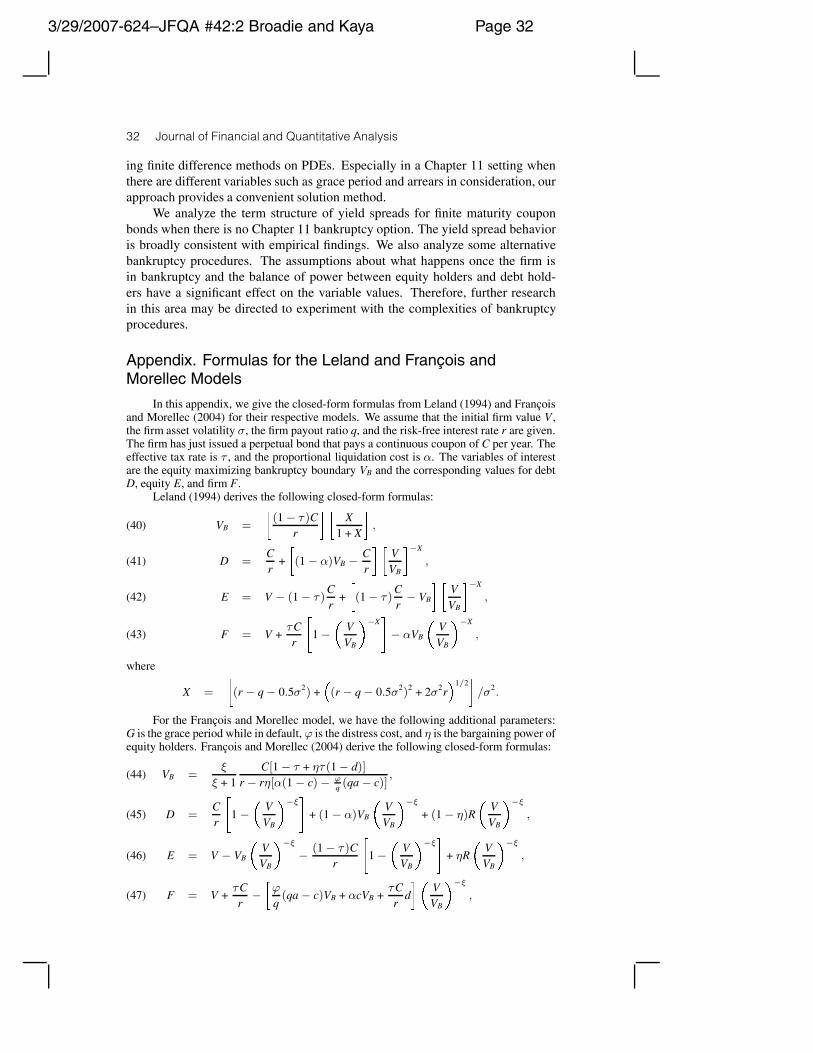
3/29/2007-624–JFQA #42:2 Broadie and Kaya Page 32
32 Journal of Financial and Quantitative Analysis
ing finite difference methods on PDEs. Especially in a Chapter 11 setting whenthere are different variables such as grace period and arrears in consideration, ourapproach provides a convenient solution method.
We analyze the term structure of yield spreads for finite maturity couponbonds when there is no Chapter 11 bankruptcy option. The yield spread behavioris broadly consistent with empirical findings. We also analyze some alternativebankruptcy procedures. The assumptions about what happens once the firm isin bankruptcy and the balance of power between equity holders and debt hold-ers have a significant effect on the variable values. Therefore, further researchin this area may be directed to experiment with the complexities of bankruptcyprocedures.
Appendix. Formulas for the Leland and Francois andMorellec Models
In this appendix, we give the closed-form formulas from Leland (1994) and Francoisand Morellec (2004) for their respective models. We assume that the initial firm value V ,the firm asset volatility σ, the firm payout ratio q, and the risk-free interest rate r are given.The firm has just issued a perpetual bond that pays a continuous coupon of C per year. Theeffective tax rate is τ , and the proportional liquidation cost is α. The variables of interestare the equity maximizing bankruptcy boundary VB and the corresponding values for debtD, equity E, and firm F.
Leland (1994) derives the following closed-form formulas:
VB =
�(1 − τ )C
r
��X
1 + X
�,(40)
D =Cr
+
�(1 − α)VB − C
r
��VVB
�−X
,(41)
E = V − (1 − τ )Cr
+
�(1 − τ )
Cr− VB
� �VVB
�−X
,(42)
F = V +τCr
�1 −
�VVB
�−X�− αVB
�VVB
�−X
,(43)
where
X =
�(r − q − 0.5σ2) +
�(r − q − 0.5σ2)2 + 2σ2r
�1/2�
/σ2.
For the Francois and Morellec model, we have the following additional parameters:G is the grace period while in default, ϕ is the distress cost, and η is the bargaining power ofequity holders. Francois and Morellec (2004) derive the following closed-form formulas:
VB =ξ
ξ + 1C[1 − τ + ητ (1 − d)]
r − rη[α(1 − c) − ϕq (qa − c)]
,(44)
D =Cr
�1 −
�VVB
�−ξ�
+ (1 − α)VB
�VVB
�−ξ
+ (1 − η)R
�VVB
�−ξ
,(45)
E = V − VB
�VVB
�−ξ
− (1 − τ )Cr
�1 −
�VVB
�−ξ�
+ ηR
�VVB
�−ξ
,(46)
F = V +τCr
−�
ϕ
q(qa − c)VB + αcVB +
τCr
d
��VVB
�−ξ
,(47)

3/29/2007-624–JFQA #42:2 Broadie and Kaya Page 33
Broadie and Kaya 33
where b = (1/σ)(r − q − 0.5σ2), λ =√
2r + b2, and ξ = (1/σ)(b + λ). In the equationsabove, we have
a =1λ
�1
λ + b + σ+
1λ − b − σ
Φ(−λ√
G)
Φ(λ√
G)
�,
c =Φ−(σ + b)
√G
Φ(λ√
G),
d =λ − b2λ
+λ + b2λ
Φ(−λ√
G)
Φ(λ√
G),
R = αVB(1 − c) − ϕ
q(qa − c)VB +
τCr
(1 − d),
Φ(x) = 1 + x√
2π exp
�x2
2
�N (x)
with N (·) the cumulative standard normal distribution function.
References
Anderson, R. W., and S. Sundaresan. “The Design and Valuation of Debt Contracts.” Review ofFinancial Studies, 9 (1996), 37–68.
Anderson, R. W.; S. Sundaresan; and P. Tychon. “Strategic Analysis of Contingent Claims.” EuropeanEconomic Review, 40 (1996), 871–881.
Anderson, R. W., and C. Tu. “Numerical Analysis of Strategic Contingent Claim Models.” Journal ofComputational Economics, 11 (1998), 3–19.
Black, F., and J. Cox. “Valuing Corporate Securities: Some Effects of Bond Indenture Provisions.”Journal of Finance, 31 (1976), 351–367.
Boyle, L. L., and S. H. Lau. “Bumping Up Against the Barrier with the Binomial Method.” Journalof Derivatives, 1 (1994), 6–14.
Brennan, M. J., and E. S. Schwartz. “Corporate Income Taxes, Valuation, and the Problem of OptimalCapital Structure.” Journal of Business, 51 (1978), 103–114.
Brezinski, C., and M. Zaglia. Extrapolation Methods: Theory and Practice. New York, NY: North-Holland (1991).
Broadie, M.; M. Chernov; and S. Sundaresan. “Optimal Debt and Equity Values in the Presence ofChapter 7 and Chapter 11.” Working Paper, Columbia University (2005).
Broadie, M., and J. B. Detemple. “American Option Valuation: New Bounds, Approximations, and aComparison of Existing Methods.” Review of Financial Studies, 9 (1996), 1211–1250.
Cox, J. C.; S. A. Ross; and M. Rubinstein. “Option Pricing: A Simplified Approach.” Journal ofFinancial Economics, 7 (1979), 229–263.
Derman, E.; I. Kani; D. Ergener; and I. Bardhan. “Enhanced Numerical Methods for Options withBarriers.” Financial Analysts Journal, 51 (1995), 65–74.
Dixit, A. K., and R. S. Pindyck. Investment under Uncertainty. Princeton, NJ: Princeton UniversityPress (1994).
Fan, H., and S. Sundaresan. “Debt Valuation, Renegotiation, and Optimal Dividend Policy.” Reviewof Financial Studies, 13 (2000), 1057–1099.
Francois, P., and E. Morellec. “Capital Structure and Asset Prices: Some Effects of BankruptcyProcedures.” Journal of Business, 77 (2004), 387–441.
Galai, D.; A. Raviv; and Z. Wiener. “Liquidation Triggers and the Valuation of Equity and Debt.”Working Paper, Hebrew University of Jerusalem (2003).
Gobet, E. “Analysis of the Zigzag Convergence for Barrier Options with Binomial Trees.” Preprint,Universite Paris VI (1999).
Leland, H. “Corporate Debt Value, Bond Covenants, and Optimal Capital Structure.” Journal ofFinance, 49 (1994), 1213–1252.
Leland, H., and K. B. Toft. “Optimal Capital Structure, Endogenous Bankruptcy, and the Term Struc-ture of Credit Spreads.” Journal of Finance, 51 (1996), 987–1019.
Merton, R. C. “On the Pricing of Corporate Debt: The Risk Structure of Interest Rates.” Journal ofFinance, 29 (1974), 449–470.

3/29/2007-624–JFQA #42:2 Broadie and Kaya Page 34
34 Journal of Financial and Quantitative Analysis
Moraux, F. “Valuing Corporate Liabilities When the Default Threshold is not an Absorbing Barrier.”Working Paper, Universite de Rennes I (2002).
Paseka, A. “Debt Valuation with Endogenous Default and Chapter 11 Reorganization.” WorkingPaper, University of Arizona (2003).
Press, W. H.; S. A Teukolsky; W. T. Vetterling; and B. P. Flannery. “Numerical Recipes in C.” Cam-bridge, MA: Cambridge University Press (1992).
Sarig, O., and A. Warga. “Some Empirical Estimates of the Risk Structure of Interest Rates.” Journalof Finance, 44 (1989), 1351–1360.