iv

A BIO-OPTICAL MODEL FOR SYRINGODIUM FILIFORME

CANOPIES

by

Margaret A. Stoughton B.S. May 2001, Virginia Polytechnic Institute and State University

A Thesis Submitted to the Faculty of Old Dominion University in Partial Fulfillment of the

Requirement for the Degree of

MASTER OF SCIENCE

OCEAN AND EARTH SCIENCES

OLD DOMINION UNIVERSITY May 2009

Approved by:

_____________________________ Richard C. Zimmerman (Director)

_____________________________ Larry P. Atkinson (Member)

_____________________________ David J. Burdige (Member)

ABSTRACT

A BIO-OPTICAL MODEL FOR SYRINGODIUM FILIFORME CANOPIES

Margaret A. Stoughton Old Dominion University, 2008

Director: Dr. Richard C. Zimmerman

Seagrasses are significant ecological and biogeochemical agents in shallow water

ecosystems throughout the world. In many regions, seagrass meadows occupy a

sufficient fraction of the coastal zone, and generate optical signatures that can be

observed from space. Bio-optical models of light absorption and scattering by

submerged plant canopies for certain species such as Thalassia testudinum and Zostera

marina have successfully modeled the plane irradiance distribution and photosynthesis

within the submerged canopies. Syringodium filiforme differs from T. testudinum and Z.

marina, in leaf morphology and canopy architecture. The objective of this study was to

develop a radiative transfer model that accurately predicts the light absorbed and

reflected by the canopy of this morphologically unique, and abundant tropical seagrass.

The approach involved modifying Zimmerman’s (2003) flat leaf bio-optical model by

incorporating the unique vertical biomass distribution of S. filiforme. Leaf length

frequency data along with the assumption of a spherical canopy allowed the

parameterization of the unique architecture of the seagrass canopy. Model predictions of

downwelling irradiance and attenuation coefficients within the Syringodium filiforme

canopies were consistent with field measurements, therefore providing a robust tool for

predicting photosynthetic performance of these seagrass canopies. Model predictions of

top of the canopy upwelling irradiances, as well as top of the canopy reflectances were

also consistent with field measurements. This predictive understanding will help to

develop global algorithms for remote sensing of the abundance and productivity of this

species that will lead to better coastal management practices.

iv

Copyright, 2008, by Margaret A. Stoughton, All Rights Reserved.

v

ACKNOWLEDGMENTS

I would like to thank Dr. Richard Zimmerman, my thesis advisor, for his guidance

and constant encouragement throughout this project, and also for his generous support for

field work, research assistantships and conferences. I would also like to thank my thesis

advisory committee members, Dr. Larry Atkinson and Dr. David Burdige for their

helpful comments and contributions. I also thank my colleagues, David Ruble, Dr.

Victoria Hill, Dr. Heidi Dierssen, Jasmine Cousins, Chris Buonassissi, Alison Branco and

Dirk Aurin, for their help with field sampling, lab work and data processing. I am also

grateful to my family for their love, support, and patience throughout my graduate

studies. I also thank my friends for their constant support and encouragement and

without whom, this endeavor would have been much harder. This research was funded

by the National Aeronautics and Space Administration (NASA).

vi

TABLE OF CONTENTS

Page LIST OF TABLES ............................................................................................................ vii LIST OF FIGURES ......................................................................................................... viii Chapter I. INTRODUCTION ................................................................................................1 II. METHODS AND MATERIALS ........................................................................5 A. THE BIO-OPTICAL MODEL OF S. FILIFORME CANOPIES ..................5 MODULE (i): VERTICAL CANOPY ARCHITECTURE AND LEAF GEOMETRY ..............................................7 MODULE (ii): RADIATIVE TRANSFER IN A SUBMERGED PLANT CANOPY ...........................................................9 MODULE (iii): CANOPY PHOTOSYNTHESIS ..................................12 PUR-BASED PREDICTIONS OF SEAGRASS DENSITIES ...............13 B. MODEL PARAMETERIZATION AND VALIDATION ...........................14 IN CANOPY IRRADIANCE PROFILES ..............................................16 WATER COLUMN OPTICAL PROPERTIES ......................................16 III. RESULTS. .......................................................................................................19 LEAF OPTICAL PROPERTIES .............................................................19 SEABED OPTICAL PROPERTIES .......................................................23 SENSITIVITY OF THE MODEL TO CANOPY ARCHITECTURE ...24 PREDICTING CANOPY REFLECTANCE AS A FUNCTION OF L ..37 CANOPY PHOTOSYNTHESIS, LIGHT-LIMITED DISTRIBUTION, DEPTH DISTRIBUTION ................................38 EFFECT OF DIFFERENT MODEL SCENARIOS AND SHOOT DENSITY ON CANOPY PRODUCTIVITY ..................40 EFFECTS OF PUR-BASED ESTIMATES OF SHOOT DENSITY AND OPTICAL DEPTH ................................................................42 IV. DISCUSSION ..................................................................................................43 V. CONCLUSION .................................................................................................50 REFERENCES ..................................................................................................................51

vii

LIST OF TABLES

Table Page 1. List of symbols with definitions and units used in the model. .............................. 6 2. ANCOVA of modeled vs. measured peak reflectances at 550 nm. ...................... 38

viii

LIST OF FIGURES

Figure Page 1. Satellite image of Florida Bay obtained by the MODIS Ocean Color Sensor (http://modis.gsfc.nasa.gov/) showing the field stations occupied in the summer of 2005 and 2006 ........................................................... 15 2a. Mean leaf absorption [aL(λ) m-1 leaf] and leaf absorptance (AL) spectra of Syringodium filiforme, Thalassia testudium and Zostera marina ........ 20 2b. Mean leaf reflectance (RL) spectra of S. filiforme, T. testudium and Z. marina .... 20 3a. Epifluorescence micrograph showing partial cross section of a Syringodium filiforme leaf .................................................................................... 22 3b. Epifluorescent micrograph showing the cross section of Thalassia testudinum leaf ..................................................................................... 22 4. Mean reflectance spectra of sediment cores collected at five Florida Bay stations where dense Syringodium filiforme canopies were observed ........... 23 5. Vertical biomass distribution of Syringodium filiforme compared to T. testudium taken near Lee Stocking Island, Bahamas (Zimmerman, 2003) ..... 25 6a. Predicted vs. measured downwelling irradiance [Ed(λ)] using original vertical biomass distribution parameters for flat strap-like leaves (sigmoid model) at the top of the canopy (550 mm, initial condition), in the middle of the canopy (350 mm), and towards the bottom of the canopy (200 mm) ........................................................................................ 26 6b. % RMS of predicted vs. measured Ed using the sigmoid biomass distribution parameters for all simulated and measured depths within the canopy ..................................................................................... 26 7a. Predicted vs. measured upwelling irradiance (Eu) using original biomass for flat strap-like leaves (Sigmoid model) ............................................................ 27 7b. % RMS of predicted vs. measured Eu using the original sigmoid biomass distribution parameters ........................................................................... 27 8. Schematic of compressed sigmoid model ............................................................. 28 9. % Leaf Biomass vs Height above the seafloor using the compressed

ix

sigmoid model and bending canopy height by 100 mm increments to obtain the vertical biomass parameters ................................................................. 29 10a. % RMS of predicted vs. measured Ed compressed at 100, 300 and 500 mm increments ............................................................................................... 31 10b. % RMS of predicted vs. measured Eu compressed at 100, 300 and 500 mm increments ....................................................................................... 31 11. Spherical model representation of canopy architecture and vertical biomass distribution within S. filiforme canopies .................................... 33 12a. Predicted vs measured downwelling irradiance (Ed) using the spherical biomass distribution parameters after the canopy was assumed to take on a spherical shape .............................................................................................. 34 12b. % RMS of predicted vs. measured (Ed) using the spherical canopy model .......... 34 13a. Predicted vs measured downwelling irradiance (Eu) using the spherical model biomass distribution parameters ................................................. 36 13b. % RMS of predicted vs. measured Eu using the spherical canopy model ............ 36 13c. Predicted vs. measured reflectance (R) at the top of the canopy .......................... 36 14. Leaf area index (L) vs peak reflectance at 550 nm (modeled and measured) ....... 38 15. Gross Photosynthesis vs. Irradiance for Syringodium filiforme ............................ 39 16. Shoot density vs. daily spectral whole-plant P:R. ................................................ 41 17. Optical depth vs modeled maximum shoot density when P:R = 1 using PUR..... 42

1

CHAPTER I INTRODUCTION

The light environment, remotely sensed reflectance, and productivity of natural

ecosystems can be estimated by applying radiative transfer theory (Verhoef & Bach,

2007) which defines the change in energy through absorption, emission and scattering as

photons are propagated through a medium. Within a plant canopy, light can change in

spectral composition as it is transmitted, absorbed and scattered by the canopy structure

(Campbell and Norman, 1998). Modeling radiative transfer processes through vegetation

is highly dependent upon the physical architecture of the plant canopy as well as

individual leaf optical properties which can vary with species and environmental

acclimation. In particular, it is necessary to determine geometric relationships between

the leaf surface and the incoming irradiance distribution because leaves are plane

irradiance collectors that obey the Cosine Law (Campbell & Norman, 1998).

The vertical distribution of leaf biomass required to model radiative transfer

through a plant canopy depends on the structure of the leaves themselves, as well as the

vertical distribution of photosynthetic biomass, which can vary dramatically among

vegetation types (Campbell, 2006). Shrubs may have a photosynthetic biomass

distribution that is, for the most part uniform from the top of the canopy to the ground.

Trees, on the other hand, may have a photosynthetic biomass distribution that is greatest

in the upper layer of the canopy and goes to zero at some distance above the ground.

The model journal for this thesis is Limnology and Oceanography

2

The photosynthetic biomass of most grasses, including Phragmites australis, and

seagrasses such as Thalassia testudinum, and Zostera marina is greatest at the base of the

canopy and decreases toward the top, creating a sigmoid shaped distribution curve

(Hirose and Werger, 1995; Zimmerman, 2003).

In aquatic habitats, light is attenuated by materials dissolved and suspended in the

medium that are independent of the submerged plant canopy (Kirk, 1994; Mobley, 1994).

Thus, a predictive understanding of radiative transfer within plant canopies submerged in

natural waters requires quantitative knowledge of the inherent optical properties of both

the water column and the plant canopy. Understanding radiative transfer in submerged

plant canopies provides the basis for calculating rates of photosynthesis and metabolic

carbon balance that determines the distribution of plant communities across the

submarine landscape and serves as the basis for remote sensing of their optically shallow

habitats (Zimmerman, 2006; Dierssen et al., 2003).

Light is one of the most crucial factors controlling the abundance and productivity

of seagrasses (Duarte, 1991). All species of seagrass have relatively high light

requirements to sustain net productivity when compared to phytoplankton or seaweeds, in

large part because they are carbon-limited (Zimmerman et al., 1997; Palacios and

Zimmerman, 2007). The high light requirements confine them to shallow waters and

makes seagrass vulnerable to eutrophication and sediment loading that decrease light

transmission to the benthos (Short and Wyllie-Echeverria, 1996). Light requirements of

seagrasses, based mostly on correlative field studies, differ among species and even

within species from different locations (Longstaff & Dennison, 1999), but the

mechanistic basis for the differences remain elusive. Therefore, a mechanistic

3

understanding of these differences can be achieved by exploring the fundamental

relationships between canopy architecture, individual leaf optical properties and the

underwater light environment.

Eutrophication of coastal environments throughout the world, subject seagrasses to

intense phytoplankton blooms and suspended sediment concentration that have the

potential to cause light limitation that diminishes seagrass habitat. In turn, this can have

significant impacts on many species of fish and invertebrates that rely on these

“ecosystem engineers” for food and shelter (Short and Wyllie-Echeverria, 1996). In the

past three decades, the Florida Bay ecosystem has been dramatically altered, and seagrass

communities have been especially hard hit. Large seagrass die-offs have been noticed

since 1987, along with an increased turbidity, resulting from ongoing algal blooms and

sediment re-suspension (Hall et al, 1999). These die offs of seagrasses or other changes

in benthic habitats have been detected from space using satellite imagery and remote

sensing, and can be used as indicators of the health of the coastal ecosystem (Dennison et

al. 1993). By using remote sensing for rapid identification of benthic features, the

prediction of detrimental factors could prove to be useful for coastal management in

optically shallow waters (Louchard et al., 2003).

Syringodium filiforme meadows can be found in a variety of environments, such as

coastal lagoons, high energy oceanic environments, or somewhat stable hydronamic

conditions throughout the southeastern United States, the Caribbean Sea, and the Gulf of

Mexico (Kenworthy and Schwarzschild, 1998). Along with Thalassia testudinum and

Halodule wrightii, S. filiforme is a major species in Florida Bay, and exists in extreme

monospecific (or nearly so) meadows along the Florida Keys. S. filiforme is unique

4

because it posses cylindrical leaves, whereas most seagrasses (i.e. T. testudinum and H.

wrightii) possess flat, strap-like leaves that present a very different optical target to

incident light. In addition to their cylindrical shape, S. filiforme leaves branch from

meristematic nodes located throughout the canopy, rather than the seafloor. This

produces a biomass distribution that is more shrub-like than the grass-like patterns of

Thalassia testudinum or Zostera marina. Modeling S. filiforme canopies therefore,

requires a different approach to estimate productivity, biomass distribution, and

vegetation abundance than used previously for seagrass morphotypes characterized by

true basal meristems (Zimmerman, 2003). The purpose of this study was to develop a

bio-optical model for S. filiforme canopies that provides a predictive understanding of the

underwater light distribution in these unique canopies and to increase our understanding

of radiative transfer processes in different types of seagrass canopies.

5

CHAPTER II

METHODS AND MATERIALS

A. The bio-optical model of Syringodium filiforme canopies:

The model was based on a two flow approach and consisted of three modules; (i)

one that simulated the architecture, including leaf geometry of S. filiforme, (ii) another

that calculated the irradiance distribution that results from light absorption and scattering

from the canopy architecture and optical properties of the leaves and water column, and

(iii) a third that calculated photosynthesis of the submerged plant canopy resulting from

light absorption by the leaves (Zimmerman, 2003). The model simulated the light

environment of a submerged canopy by dividing the canopy volume, including the leaves

and the water column, into a series of horizontal sections of finite thickness (∆z). The

optical properties of each section were based on the architecture of the canopy, the

orientation and optical properties of the leaves, and the optical properties of the dissolved

materials and suspended particles in the water column. Some parameters in the model

were wavelength and/or depth dependent as indicated by the parenthetic notation; (λ, z).

Symbol definitions and their dimensions are listed in Table 1.

6

Table 1. List of symbols with definitions and units used in the model. Symbol Definition Dimensions Basic parameters z Depth within the canopy m μ Average cosine of plane irradiance distribution Dimensionless θ Polar angle of plane irradiance Degrees Canopy architecture B(z) Biomass fraction in each canopy layer (z) Dimensionless B Nadir bending angle of the seagrass canopy Degrees h(z) Height above the seafloor m

L Canopy leaf area index m2 m-2

l(z) Leaf area index at depth z m2 m-2

lp(z) Horizontally projected leaf area at depth z m2 m-2

tL Leaf thickness m y height of individual layer within canopy m D height of the canopy m Irradiance within canopy

Ed (λ,z) Downwelling plane irradiance W m-2nm-1

Eu (λ,z) Upwelling plane irradiance W m-2nm-1 Leaf and Canopy optical properties

aL (λ) Leaf absorption coefficient m-1 leaf thickness

AL (λ) Leaf absorptance Dimensionless

DL (λ) Leaf absorbance Dimensionless

RL (λ) Leaf reflectance Dimensionless

Rb (λ) Bottom reflectance of seabed Dimensionless

Ru(λ) Canopy reflectance of upwelling irradiance Dimensionless

RTOC(λ) Top of the canopy reflectance Dimensionless Apparent optical properties of the water column

Kd (λ) Water column attenuation of Ed m-1

Ku (λ) Water column attenuation of Eu m-1 Metabolic parameters Ek Light saturation parameter mol photon m-2 sec-1

α Initial slope of P vs. E curve mol O2 evolved mol-1 photon incident

R Respiration rate mol CO2 m2 min-1

PAR(z) Photosynthetically available irradiance in layer z incident photon m-2 leaf

PUR (z) Photosynthetically used irradiance in layer z quanta absorbed m-2 leaf

φp Quantum yield of photosynthesis mol O2 evolved mol-1 quanta absorbed

Pi (z) Biomass-specific photosynthesis in layer z dimensionless

7

Module (i): Vertical canopy architecture and leaf geometry The canopy architecture, leaf orientation and shoot density of six Syringodium

filiforme populations from Florida Bay were measured in June and July 2006. Shoot

density was determined using approximately 20 randomly located quadrats (0.01 m2) at

each station. One shoot consisting of all leaves attached to a single rhizome was collected

from each quadrat for subsequent determination of shoot morphology and leaf optical

properties. The total surface area per shoot, the number of leaves per shoot, and the

maximum length and width of the leaves were measured in the laboratory using a plastic

meter tape and digital caliper.

The leaf area index (L) of the entire canopy was divided into a series of fractional

leaf area indices l(z) for each depth interval (z) as:

l(z) = L x B(z) (1)

where, L represents the leaf area index for the entire canopy, and B(z) represents the

relative biomass at depth z. The relative biomass [B(z)] varies at each depth for different

species of seagrass and becomes the primary focus for modeling the unique canopy

architecture of S. filiforme.

The leaf area index (L) for thin flat leaves (such as turtlegrass and eelgrass), is the

silhouette, or one-sided area of leaves per unit ground surface area. This leaf area index

is also useful for the cylindrical leaves of S. filiforme because the shadow area of a

cylindrical leaf would be identical to that of a flat, strap like leaf of the same width. Even

though the shape and structure of the leaves do not change the calculation of leaf area

index, the distribution of leaf origin produces a unique biomass distribution within the S.

filiforme canopy. The tall and hollow leaves of S. filiforme originate at various locations

8

throughout the canopy, creating a biomass distribution that is considerably different from

other seagrasses in which all leaves emerge from a single meristem in the base of the

shoot at the seafloor.

Leaf orientation relative to the downwelling and upwelling irradiance planes

within the canopy was also accounted for in the model. Unlike phytoplankton, which are

scalar irradiance collectors that harvest light equally from all directions, seagrasses are

plane irradiance collectors in which the geometric orientation of the leaf has a predictable

impact on the light incident on, and therefore, absorbed by the leaf. This relationship is

defined by the Cosine Law, which states that the irradiance incident on a plane surface is

proportional to the cosine of the angle between the photon direction and the surface

normal (Zimmerman & Dekker, 2006). Leaf area index [l(z)] within each vertical section

(z), was corrected for orientation by calculating the horizontally projected leaf area [lp(z)]

as a function of the nadir bending angle (β) of the leaves in each depth interval:

lp(z) = l(z) sinβ(z) (2)

Also, because seagrass leaves are plane irradiance collectors, the horizontally projected

optical target must be adjusted for the angular distribution of the downwelling or

upwelling irradiance. The cosine law defines this correction as [lp(z)]/cosθ] for a

collimated beam, where θ represents the zenith angle of the beam incident on lp(z). Even

though the downwelling light in natural environments is not a collimated beam, its

angular distribution can be approximated using the average cosine ( dμ ):

dμ = Ed/E0d (3)

where Ed represents downwelling plane irradiance and E0d represents the downwelling

scalar irradiance. The relationship between seagrass leaves and downwelling irradiance

9

was approximated by replacing the average cosine for cos θ and using the ratio [lp(z)/

dμ (z)] as the geometric correction factor (Zimmerman, 2003).

Module (ii): Radiative transfer in a submerged plant canopy

Leaf optical properties (reflectance, transmittance, absorbance, and absorptance)

of the cylindrical S. filiforme leaves were measured across the visible and NIR spectrum

(400-800 nm) using an ASD Field Spec Pro spectrophotometer fitted with an integrating

sphere and tungsten lamp. Because S. filiforme leaves were narrower than the opening to

the integrating sphere, the estimation of leaf optical properties (LOP’s) required use of

the composite method (Daughtry, 1989), which consisted of carefully arranging four

leaves in a custom-made sample holder that separated the leaves by open gaps, across the

integrating sphere, and determining the fractional area of the optical window occluded by

the leaves. Measured spectral absorbances [D(λ)] and reflectances [R(λ)] were then

corrected by the fractional shadow area to obtain true leaf absorbances [DL(λ)] and

reflectances [RL(λ)]. Leaf absorbances were measured by placing the leaf sample at the

entrance of the integrating sphere between the light source and the sphere. Leaf

reflectance was measured by placing the leaves at the back of the integrating sphere so

that all of the light scattered backward from the leaf surface was captured inside the

sphere. Dependence of DL(λ) on fractional area occupied by the leaves was determined

with 2, 3 and with 4 leaves placed in the sample holder, resulting in a linear relationship

between absorption and shadow area (cm2), (slope = 0.039, r2 = 0.98, n = 4).

10

Spectrophotometric leaf absorbances [D(λ)] were then converted into raw

absorptance [Araw(λ)] :

Araw(λ) = 1 - 10-D(λ) (4)

and corrected for reflectance [RL(λ)] to get true leaf absorptances [AL(λ)]:

AL(λ) = Araw(λ) - RL(λ) (5)

Corrected leaf absorptances, were converted into length-specific absorption spectra using

the cross-sectional thickness of the leaf (tL) measured using a digital caliper:

aL(λ) = -ln [1 - AL(λ)] / tL (6)

The downwelling and upwelling plane irradiance emerging from each horizontal

cross-section of the canopy were then determined by incorporating the leaf optical

properties into a two flow model of plane irradiance distribution within the canopy.

Downwelling irradiance was calculated using the Lambert-Beer Law:

Ed (λ, z) = Ed (λ, z-1)[1-Rd(λ, z)]

× exp [-Kd(canopy)(λ, z) - Kd(water)(λ, z)Δz] (7)

where Ed (λ, z-1) represents the downwelling plane irradiance incident on layer z from

layer (z-1) above, [1-Rd(λ, z)] represents the loss term of upward reflection of the

downwelling irradiance in each layer (z). Rd(λ, z) was determined from the leaf

reflectance [RL(λ)] measured spectrophotometrically in the lab, the horizontally projected

leaf area in layer (z), and the average cosine of the downwelling irradiance [lp(z) / dμ (z)]:

Rd(λ, z) = RL(λ) [lp(z) / dμ (z)] (8)

Light attenuation by the canopy [Kd(canopy)(λ,z)] was calculated from the exponential term

[aL(λ) ×tL × (lp(z)) / dμ )] which incorporates the leaf optical properties within the

seagrass canopy where aL(λ) is the geometric absorption coefficient (m-1) for

11

Syringodium filiforme leaves (Equation 6), tL is the thickness of the leaves (m), and

(lp(z)/ dμ ) is the geometric correction factor as described above for Rd(λ, z). The very last

part of the equation [Kd(water)(λ, z)Δz] describes light attenuation by the water column and

represents the downwelling attenuation coefficient in each layer of the horizontally

divided water column and the thickness of each layer in the water column (Δz).

Upward propagation of Eu (λ, z) was calculated by reflecting the downwelling

irradiance off of the bottom and propagating it back up through the canopy layers in a

manner symmetrical to the downward propagation of Ed(λ, z), (Zimmerman, 2003):

Eu (λ, z) = {[Ed (λ, z)Rd(λ, z +1)] + Eu (λ,z + 1)}

× [1 – Ru(λ, z)]

× exp [-Ku(canopy)(λ,z) - Ku(water)(λ,z)Δz] (9)

where, [Ed (λ, z + 1)] represents the downwelling irradiance reflected back up through

layer z, 1– Ru(λ, z) represents the reflected loss of upwelling light, Eu (λ, z + 1) represents

the upwelling irradiance transmitted through each layer z, Ku(water)(λ,z) represents the

upwelling attenuation coefficient for the water column and was derived from Kd(water)(λ, z)

by propagation of light from the seabed upward through the canopy with the assumption

that the seabed represented a Lambertian reflecting boundary (i.e. equal radiances at all

hemispheric angles):

Ku(water)(λ, z) = Kd(water)(λ, z) ( , )0.5

zμ λ (10)

Top of the canopy reflectance (RTOC) was calculated by normalizing the predicted

upwelling irradiance emanating from the canopy to the downwelling irradiance incident

on the top layer of the canopy where z is equal to zero:

RTOC (λ,z) = Eu(λ,z0) /Ed(λ,z0) (11)

12

Module (iii): Canopy photosynthesis

The photosynthetic absorptance [Ap(λ)] was calculated by removing the mean

absorption between 710 and 750 nm from LA (λ) (defined in Equation 5):

Ap(λ) = AL(λ) - LA (710-750) (12)

The photosynthetically utilized radiation (PUR) was then calculated for each canopy

layer (z) using photosynthetic leaf absorptance, horizontally projected leaf area and

upwelling and downwelling irradiances:

d up p

d u

( , 1) ( , 1)( ) ( ) ( )( 1)

E z E zPUR z A l zzλ

λ λλμ μ

⎡ ⎤− += +⎢ ⎥−⎣ ⎦

∑ (13)

Instantaneous biomass-specific gross photosynthesis within layer (z) [(Pi(z)) (μmol

O2 m-2 min-1)] was calculated using a cumulative one-hit Poisson function (Falkowski

and Raven, 1997) to provide a general context for evaluating the effects of canopy

orientation and leaf optical properties on the potential for photosynthetic light use:

Pi(z) = B(z)Pm{1-exp[-φp x PUR(z)]} (14)

where, B(z) represents the biomass fraction found in layer z, and, φp represents the

quantum yield of photosynthesis (mol C fixed mol-1 photons absorbed). The quantum

yield of photosynthesis (φp, mols O2 evolved mol-1 photons absorbed) was determined by

the measured relative spectral distribution from the light source and from that, converted

PAR measurements to PUR. In normalizing the photosynthesis versus irradiance (P vs.

E) curves to Pm, the light use efficiency (φp) became an aggregate term with units of (m2

leaf s)/(quanta absorbed) and Pi(z) became a dimensionless factor that ranged from 0 to

B(z).

13

The normalized rate of biomass-specific instantaneous photosynthesis for the whole

canopy (Pc) was then determined by summation of Pi(z) over z:

Pc=Σz Pi(z) (15)

PUR-based predictions of seagrass densities

Predictions of a range of sustainable seagrass densities were estimated using the

absorbed light (photosynthetically utilized radiation, PUR), that depended on Pm, φp and

Ap. Biomass-specific gross photosynthesis was determined from the P vs. E curves to

provide a basis for relating the leaf orientation within the canopy and the optical

properties of the leaves to whole-canopy photosynthesis.

Sustainable seagrass densities were defined as the density at which photosynthesis

equals respiration and PAR-based calculations for the diffuse attenuation [KPAR] were

determined as:

700

400700

400

( )

(0)ln

d

d

PAR

E z

EK

z

λ

λ

=

=

⎛ ⎞⎜ ⎟⎜ ⎟⎜ ⎟⎜ ⎟⎝ ⎠= −

∑

∑ (16)

where, K(λ) represents the spectral average of the Kd (λ), and λ represents the number of

wavelengths. The optical depth for S. filiforme canopies was then found as:

ζ = KPAR · z (17)

where z equals the depth at the base of the canopy.

14

Sustainable seagrass densities were defined as the density at which whole plant

photosynthesis equals respiration (P:R = 1) on a 24 hour basis, as described by

Zimmerman et al. (1997).

B. Model parameterization and validation

Data to validate the model were obtained during two summer field seasons in the

Florida Keys in 2005 and 2006 (Fig. 1). Stations north of the Keys represented by the

green circles indicate the presence of dense meadows of S. filiforme in the relatively

turbid waters of Greater Florida Bay. The blue squares represent sand, the pink inverted

triangles represent meadows of T. testudinum. All stations north of the Keys ranged from

1-2 meters in depth. The red diamonds represent oceanic stations south of the Keys

where patchy meadows of T. testudinum and H. wrightii were present in 7-10 meters of

water.

Seabed reflectance spectra [Rb(λ)] were measured in the lab on sediment cores

collected from the S. filiforme meadows using a plastic coring cylinder driven into the

seabed. The core was then extracted from the sediment along with a few centimeters of

the overlying water column and taken back to the laboratory for analysis. Cores were

extruded using a worm gear plunger to expose the upper surface layer and remove the

overlying water column. Measurements of sediment reflectance were measured using a

tungsten light source and ASD spectrophotometer calibrated using a Spectralon (99.9%

reflectance) plaque. The reflectance spectra were used to define bottom reflectance

[Rb(λ)] in the model runs.

15

Figure 1. Satellite image of Florida Bay obtained by the MODIS Ocean Color Sensor

(http://modis.gsfc.nasa.gov/) showing the field stations occupied in the summer of 2005

and 2006. Circles indicate dense meadows of Syringodium filiforme.

Digital light micrographs of individual leaf cross sections of S. filiforme and T.

testudinum were taken with an Axiovert 40 CFL microscope (100x). The cross sections

were hand cut using a razor blade, wet-mounted in seawater and illuminated with

epifluroescent light (blue excitation) to stimulate chlorophyll a fluorescence of

chloroplasts with an X-Cite series 120 fluorescence illumination lamp.

Sand Thalassia testudinum Syringodium filiforme Oceanside

16

In canopy irradiance profiles

Profiles of spectral downwelling and upwelling irradiance through S. filiforme

canopies were collected using the DOBBS (Diver Operated Benthic Bio-Optical

Spectrophotometer), a radiometrically calibrated three-channel HydroRad (HOBI Labs)

mounted on a portable frame that was easily manipulated by a SCUBA diver to take in

situ irradiance measurements with canopies of submerged vegetation. Two of the plane

irradiance sensors were mounted on an adjustable wand that could be positioned

vertically from 0 to 1.5 meters above the sea floor, providing profiles of downwelling

plane irradiance [Ed (λ, z)] and upwelling plane irradiance [Eu (λ, z)] within the plant

canopy. The third irradiance channel was maintained at a fixed height above the plant

canopy to provide reference correction for temporal variation in Ed(λ) incident on the

canopy during the collection of in-canopy irradiance profiles. The raw in canopy spectra

(0.3 nm resolution) were interpolated to 1 nm intervals using a cubic spline and smoothed

using a 10 nm boxcar running average for validation against the model and adjusted for

any temporal variation in Ed(λ,0) above the canopy.

Water column optical properties:

Values of Kd (λ, z) and μ for the water column were obtained using an HR4 field

Spectroradiometer (HydroRad 4 Spectroradiometer HOBI Labs, Inc.) fitted with two

Gershun sensors and two plane irradiance sensors. The HR4 was mounted on a portable

frame and placed on the seafloor in a clear area away from the seagrass canopy. Two of

the Gershun sensors were located 1 meter above the sea floor and measured downwelling

17

[E0d(λ)] and upwelling [E0u(λ)] scalar irradiance. Total scalar irradiance was then

calculated:

E0 (λ) = E0d(λ) + E0u(λ) (18)

One of the two plane irradiance sensors (Ed2) was located beside the Gershan sensors; the

other was located 1 meter below Ed2 (Ed1). The coefficient of downwelling light

attenuation [Kd(λ)] was then calculated from Beer’s Law as:

d1

d2( )

( )ln( )( )d water

EEKz

λλλ

−= (19)

where the vertical distance between the two sensors (z) was 1 m. The average cosine of

the zenith angle of all downwelling light ( dμ ) (Kirk, 1994) was then calculated as:

dd

0d

( )( )

EE

λμλ

= (20)

Irradiance measurements from each of the four sensors were recorded at 0.35 nm

increments every 5 minutes. The values of Kd(water) (λ) taken at each station, along with

the Ed (λ, TOC) values taken from the DOBBS at each station at the top of the canopy

were used to initialize the model runs (Eq. 7).

Photosynthesis and respiration of individual leaf (photosynthetic tissue) and

respiration of non-photosynthetic segments rhizome segments were measured using a

temperature-controlled polarographic oxygen electrode system filled with 5 ml of 0.2 µm

filtered seawater. Leaf segments were first incubated in total darkness to measure

respiration, and then exposed to a range of increasing light intensities created using

neutral density filters and a tungsten fiber-optic light source and calibrated using a

Biospherical PAR sensor. Rates of oxygen consumption/evolution at each light level

18

were calculated as the time-rate-of-change from linear portions of the digitally recorded

oxygen concentration time series.

Metabolic data were fit to the cumulative one hit Poisson function:

P = Pm (1 - e -αE/Pm) – R (21)

where Pm represents the maximum, or light saturated rate of gross photosynthesis, E

represents the incident irradiance (PAR), α represents the light-limited slope of the P vs.

E curve, and R represents dark respiration. The P vs. E curve parameters (Pm, α and R)

were estimated using a direct fit algorithm for non-linear models implemented using

Sigma Plot 10.0 that provided objective error estimates (Zimmerman et al., 1987) and

were compared to model output estimates. The quantum yield of photosynthesis (φp) was

calculated by first converting PAR to E(λ) and PUR was then determined from Equation

13. Finally, P vs. PUR was plotted just like the P vs. E curves and (φp) was determined

as the slope of the linear portion of the curve.

The modeled upwelling and downwelling irradiances were compared to field

measurements of in-canopy Ed(λ,z) and Eu(λ,z) obtained by the DOBBS at discrete

locations within the canopy using % RMS (root mean square) error:

2

1

1 ( ( ) ( )% 100( )

n DOBBS ModeledRMS xn DOBBSλ

λ λλ=

−= ∑ (22)

where n equals the number of wavelengths, DOBBS (λ) is the measured Ed(λ) taken from

the field measurements and Modeled(λ) is the predicted Ed(λ).

19

CHAPTER III

RESULTS

Leaf optical properties:

The mean absorption (aL) and absorptance spectra (AL) of S. filiforme was

quantitatively similar to flat-leaf species, such as T. testudinum and Z. marina, in the blue

(400-500 nm) and red (600-700 nm) portions of the visible spectrum (Fig. 2a). However,

the S. filiforme spectrum was two to three times more absorbent in the green (500-650

nm), and therefore less spectrally sensitive (optically gray) than is typical of most green

plant leaves, including other seagrasses like T. testudinum and Z. marina. Although the

leaves of S. filiforme absorb about 75% of the incident light, the photosynthetic pigments

are responsible for only about 22% of the absorption. In contrast, T. testudinum absorbs

about 46% of the incoming light, and 31% of the incident light is absorbed by

photosynthetic pigments. Z. marina absorbs about 63% of the incoming light and 46% is

absorbed by the photosynthetic pigments.

Despite the differences in absorption spectra, leaf reflectance spectra (RL) of S.

filiforme were virtually indistinguishable from T. testudinum, and Z. marina (taken from

Zimmerman, 2003) across most of the spectrum. There was a clear peak in the green

between (500-600 nm) and a distinct “red edge” starting at 700 nm and extending to the

near infrared (NIR) (Fig. 2b). T. testudinum leaves, however, were slightly more

reflective in the green, (525 to 650 nm).

20

a L (m

-1 le

af)

0

2000

4000

6000

8000

10000

12000

AL

Wavelength (nm)400 500 600 700

RL

0.02

0.04

0.06

0.08

0.10

0.12

0.14

0.16

0.18

0.20

Zostera marinaThalassia testudinumSyringodium filiforme

a.

b.

8.2580E-01

9.6900E-01

9.9470E-01

9.9960E-01

9.9980E-01

9.9997E-01

Figure 2. (a) Mean leaf absorption [aL(λ) m-1 leaf] and leaf absorptance (AL) spectra of

Syringodium filiforme, Thalassia testudium and Zostera marina. (b) Mean leaf

reflectance (RL) spectra of S. filiforme, T. testudium and Z. marina. Data from T.

testudinum and Z. marina are from Zimmerman (2003).

21

Epiflouresent cross sections of S. filiforme and T. testudinum revealed the

chloroplasts (fluorescent red bodies) within S. filiforme to be widely dispersed in the

epidermal layer and mesophyll up to three cell layers away from the leaf surface, which

comprises about 47% of the total leaf volume whereas, chloroplasts within T. testudinum

and most other flat-bladed seagrasses are packed into two single-cell layers of the

epidermis comprising only about 27% of the total leaf area (Fig. 3). The cross section of

S. filiforme also reveals that about 44% of the volume was devoted to large air lacunae

(buoyant air channels) whereas the lacunae within T. testudinum comprise only about

12% of the leaf volume. These large air spaces may increase light refraction within the

leaf, increasing the probability of light absorption (Lee, 1986).

22

Figure 3. (a) Epifluorescence micrograph showing partial cross section of a Syringodium

filiforme leaf. Chloroplasts appear as bright objects within the outermost three layers of

cells. (b) Epifluorescent micrograph showing the cross section of Thalassia testudinum

leaf. Chloroplasts were almost completely restricted to the outermost epidermal cell

layer.

300 μm

23

Seabed optical properties:

Reflectance spectra [Rb(λ)] of the seabed below the S. filiforme canopies had

qualitatively similar shapes across all stations, with [Rb(λ)] increasing from blue to red

(Fig. 4). Peak reflectance at 640 nm ranged from about 0.12 to 0.26 which was about

half of the bottom reflectance for the highly reflective ooitic carbonate sand reported by

Zimmerman, (2003) (~0.45 at 650 nm). The spectra also exhibited a distinct dip at 670

nm, probably due to absorption by chlorophyll containing microalgae growing on the

sediment surface.

Wavelength (nm)400 450 500 550 600 650 700

Seab

ed R

efle

ctan

ce [R

b(l)]

0.05

0.10

0.15

0.20

0.25

0.30

0.35FBOP0601FBOP0602 FBOP0606FBOP0609FBOP0615

Figure 4. Mean reflectance spectra of sediment cores collected at five Florida Bay

stations where dense Syringodium filiforme canopies were observed.

24

Sensitivity of the model to canopy architecture:

The first simulation of canopy structure and biomass distribution for S. filiforme

canopies followed a sigmoid model, in which most of the biomass was located at the

seafloor and decreases exponentially upward to the top of the canopy:

( )( )1

sB zh z

I

ψ=

⎡ ⎤+ ⎢ ⎥⎣ ⎦

(23)

B(z) represents the relative biomass in layer z of the canopy, ψ is the fraction of biomass

at the seafloor, [h(z)] is the height above the seafloor, I represents the intermediate point

within the canopy where the curve shifts from concave to convex, and s represents the

exponential shape factor (Zimmerman, 2003). Values of ψ, I, and s were fitted to vertical

biomass distributions derived from leaf size-frequency data for all stations taken in 2005

and 2006 (Fig. 5). From this point on, FBOP0606 will be used as an example station, for

simplicity, because results from other stations were similar to this station.

25

% Leaf Biomass

0 1 2 3 4 5

Hei

ght a

bove

seaf

loor

(mm

)

0

200

400

600

800 Thalassia testudium (B(z))Syringodium filiforme (B(z))Sigmoid function

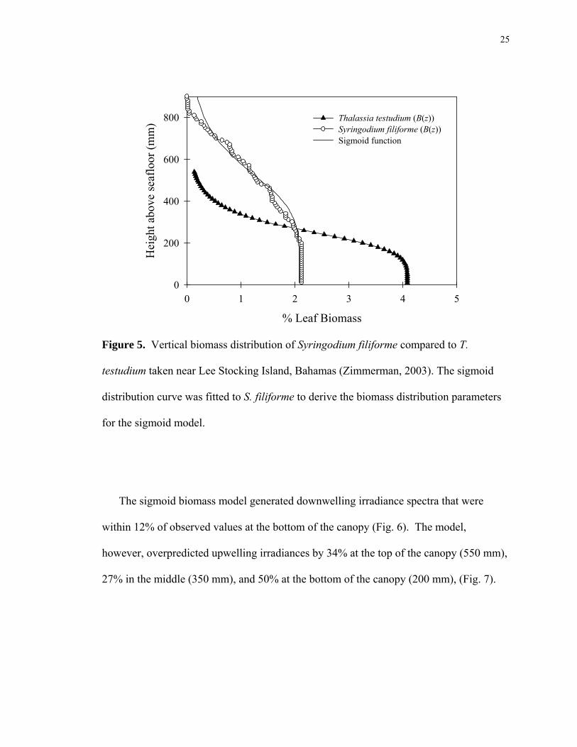
Figure 5. Vertical biomass distribution of Syringodium filiforme compared to T.

testudium taken near Lee Stocking Island, Bahamas (Zimmerman, 2003). The sigmoid

distribution curve was fitted to S. filiforme to derive the biomass distribution parameters

for the sigmoid model.

The sigmoid biomass model generated downwelling irradiance spectra that were

within 12% of observed values at the bottom of the canopy (Fig. 6). The model,

however, overpredicted upwelling irradiances by 34% at the top of the canopy (550 mm),

27% in the middle (350 mm), and 50% at the bottom of the canopy (200 mm), (Fig. 7).

26

Wavelength (nm)

400 450 500 550 600 650 700

E d (W

m-2

nm-1

)

0.0

0.2

0.4

0.6

0.8

1.0

1.2

1.4

1.6550 mm (predicted)350 mm (predicted)200 mm (predicted)550 mm (measured)350 mm (measured)200 mm (measured)

% RMS

0 2 4 6 8 10 12 14

Can

opy

Hei

ght (

mm

)

100

200

300

400

500

600

a.

b.

Figure 6. (a) Predicted vs. measured downwelling irradiance [Ed(λ)] using original

vertical biomass distribution parameters for flat strap-like leaves (sigmoid model) at the

top of the canopy (550 mm, initial condition), in the middle of the canopy (350 mm), and

towards the bottom of the canopy (200 mm). (b) % RMS of predicted vs. measured Ed

using the sigmoid biomass distribution parameters for all simulated and measured depths

within the canopy.

27

Wavelength (nm)

400 450 500 550 600 650 700

E u (W

m-2

nm

-1)

0.00

0.02

0.04

0.06

0.08

0.10

0.12550 mm (predicted)350 mm (predicted)200 mm (predicted)550 mm (measured)350 mm (measured)200 mm (measured)

% RMS

15 20 25 30 35 40 45 50 55

Can

opy

Hei

ght (

mm

)

100

200

300

400

500

600

a.

b.

Figure 7. (a) Predicted vs. measured upwelling irradiance (Eu) using original biomass for

flat strap-like leaves (Sigmoid model). (b) % RMS of predicted vs. measured Eu using

the original sigmoid biomass distribution parameters.

Although the average recorded length for S. filiforme shoots measured in the

laboratory was 754 mm, the realized average height of the submerged canopies was only

550 mm. Consequently, a set of biomass coefficients were created to compress the

canopy by bending the leaves at several different heights from 0 to 550 mm above the

28

bottom causing the leaves in the upper layer to be denser and more horizontal than below

the bending point (Fig. 8). Compression of the canopy at each 100 mm increments

therefore provided biomass distributions that were much different than the fully extended

sigmoid model (Fig. 9).

Figure 8. Schematic of compressed sigmoid model. To increase the accuracy of the Eu

predictions from the model, new biomass coefficients were created by compressing the

height of the canopy at 100 mm intervals where β represents the bending angle. Biomass

distribution parameters were derived using the sigmoid model with compression of h(z),

thereby altering the intermediate point (I) as well as the shape factor (s). These

parameters were then applied to the compression model runs.

29

% Leaf Biomass

0 1 2 3 4 5 6

Hei

ght a

bove

the

seaf

loor

(mm

)

0

200

400

600

800B(z) of S. filiforme500 mm sigmoid function400 mm sigmoid function300 mm sigmoid function200 mm sigmoid function100 mm sigmoid function

Figure 9. % Leaf Biomass vs Height above the seafloor using the compressed sigmoid

model and bending canopy height by 100 mm increments to obtain the vertical biomass

parameters.

The biomass distribution parameters were derived using the same sigmoid model as for

the fully extended (754 mm) canopy and applied to each of the model runs. However,

bending the canopy at 100 mm increased the underprediction of Ed to 78% and 97% RMS

in the middle and bottom of the canopy, respectively (Fig. 10a). Bending at 300 mm

further increased the underprediction of Ed to 96% and 93% RMS in the middle and

bottom of the canopy, respectively (Figure 10a). Bending at 500 mm reduced the

30

underprediction of Ed to 54% and 32% RMS in the middle and bottom of the canopy,

respectively (Figure 10a). Bending at 500 mm also resulted in a better prediction of Ed at

the middle and bottom of the canopy compared to bending at 100 mm and 300 mm.

Bending the biomass at 100 mm also increased the underprediction of the Eu at the top,

middle and bottom of the canopy (Figure 10b), relative to the fully extended (754 mm)

sigmoid model. Bending at 300 mm also underpredicted Eu by 37%, 79%, and 97% in

the top, middle and bottom of the canopy, respectively (Figure 10b). Bending the canopy

at 500 mm reduced the underprediction of Eu at the top, middle and bottom by 2% (Fig.

10b.) As with the Ed, the bending at 500 mm resulted in a better prediction of Eu in the

middle and bottom of the canopy when compared to bending at 100 mm and 300 mm.

These results indicate that the model is sensitive to changes in biomass

distribution resulting from differences in canopy height and bending position. Further,

bending this canopy at 500 mm rather than 100 mm or 300 mm, resulted in more accurate

predictions of irradiance distribution especially within the middle and bottom portions of

the canopy. Overall, the compressed sigmoid model did not simulate the Ed and Eu as

well as the fully extended sigmoid model despite the fact that it more accurately

represented the true height of the submerged plant canopy.

31

% RMS0 20 40 60 80 100 120

Can

opy

Hei

ght (

mm

)

200

300

400

500 Bent at 100 mmBent at 300 mmBent at 500 mm

Can

opy

Hei

ght (

mm

)

200

300

400

500 Bent at 100 mmBent at 300 mmBent at 500 mm

Ed

Eu

a.

b.

Figure 10. (a) % RMS of predicted vs. measured Ed compressed at 100, 300 and 500

mm increments. (b) % RMS of predicted vs. measured Eu compressed at 100, 300 and

500 mm increments.

The undifferentiated branching architecture of S. filiforme suggests that its canopy

is geometrically different from most of the seagrasses, including T. testudinum and Z.

marina, on which the sigmoid distribution was based. Unlike the sigmoid model, which

assumes all leaves originate at the seafloor, the leaves of S. filiforme originate at branch

32

points throughout the canopy, which distributes a larger fraction of biomass in the middle

and upper portions of the canopy (Fig. 11). To simulate this spherical distribution, the

relative biomass distribution [B(z)] within each vertical layer of the canopy was

calculated from the partial volume (V1) of a sphere where, y1 represents the height (m) of

an individual layer in the spherical canopy, and D represents the height (or diameter) of

the entire spherical canopy:

V1 = π/3 × y12 × (1.5D – y1), (24)

V2 = π/3 × y22 × (1.5D – y2), (25)

B(z) = ΔV1 – ΔV2 (26)

The resulting fractional biomass within each vertical layer of the canopy [B(z)] was

calculated by subtracting the partial volume of the sphere (ΔV) below the layer from the

volume including the layer (Figure 11):

B(z) = 4.57×10-7 + 9.10×10-5 x h +-1.14×10-7 x h2 (27)

where, h represents the height of the canopy in mm. As with previous simulations using

the sigmoid distribution, canopy height was constrained to 550 mm to correspond to

heights observed in the field.

33

Figure 11. Spherical model representation of canopy architecture and vertical biomass

distribution within S. filiforme canopies. Relative biomass distribution [B(z)] within each

vertical layer was calculated by using the partial volume (V1) of a sphere where, y1

represents the height (mm) of an individual layer in the canopy (or sphere), and D

represents the height of the entire canopy or sphere. The vertical biomass distribution was

then fit to a second order polynomial curve (bold line).

Both modeled and measured Ed (λ, z) decreased down through the canopy (Fig. 12a).

The model generated % RMS errors of Ed of 23% and 17.5% in the middle (350 mm) and

the bottom (200 mm) of the canopy, respectively (Fig 12b). The model also under

predicted the Ed in the middle and the RMS error of 23% was considerably higher than

the original sigmoid model simulating the 800 mm canopy. However, the RMS error for

34

Ed was 54% less than the compressed sigmoid model bent at 100 mm, 69% less than the

compressed sigmoid model bent at 300 mm, and was 30% less than the compressed

sigmoid model bent at 500 mm. The spherical model also slightly under predicted the Ed

at the bottom (200 mm) of the canopy but the RMS error of 18%, was only 6% higher

than the original sigmoid model and 78% less than the compressed sigmoid model bent at

100 mm, 75% less than the compressed sigmoid model bent at 300 mm, and was 14%

less than the compressed sigmoid model bent at 500 mm (Fig. 12b).

Wavelength (nm)400 450 500 550 600 650 700

E d (W

m-2

nm-1

)

0.0

0.2

0.4

0.6

0.8

1.0

1.2

1.4

1.6 550 mm (predicted)350 mm (predicted)200 mm (predicted)550 mm (measured)350 mm (measured)200 mm (measured)

% RMS0 5 10 15 20 25 30

Can

opy

Hei

ght (

mm

)

200

300

400

500

600

a.

b.

Figure 12. (a) Predicted vs measured downwelling irradiance (Ed) using the spherical

biomass distribution parameters after the canopy was assumed to take on a spherical

shape. (b) % RMS of predicted vs. measured (Ed) using the spherical canopy model.

35

Modeled upwelling irradiance (Eu) (Fig. 13a) was in best agreement with the

measured upwelling irradiance at the top of the canopy. The % RMS error of 21% (Fig.

13b) was 13% less than the fully extended sigmoid model, and about 16% less than the

compressed sigmoid models bent at 100, 300 and 500 mm, indicating that using the

spherical model will best predict upwelling irradiance at the top of the canopy. The

modeled upwelling irradiance in the middle of the canopy over predicted Eu relative to

field measurements, with a % RMS error of 82%, which was 55% greater than the fully

extended sigmoid model, and 24% less than the compressed sigmoid model bent at 100

mm, 4% greater than the compressed sigmoid model bent at 300 mm, and was 58%

greater than the compressed sigmoid model bent at 500 mm. The modeled Eu (λ, z) at the

bottom of the canopy was 184% higher than the measured and had a % RMS value that

was higher than the original sigmoid model by 134% and also higher for the compressed

model bent at 100 mm, 300 mm and 500 mm with a difference of 86%, 88%, and 126%

respectively.

36

Wavelength (nm)

400 450 500 550 600 650 700

E u (W

m-2

nm-1

)0.00

0.02

0.04

0.06

0.08

0.10550 mm (predicted)350 mm (predicted)200 mm (predicted)550 mm (measured)350 mm (measured)200 mm (measusred)

% RMS of Eu

0 20 40 60 80 100 120 140 160 180 200

Can

opy

Hei

ght (

mm

)

200

300

400

500

600

a.

b.

Wavelength (nm)

400 450 500 550 600 650 700

Ref

lect

ance

(rel

ativ

e)

0.01

0.02

0.03

0.04

0.05

0.06550 mm (predicted)550 mm (measured)

c.

Figure 13 (a) Predicted vs measured downwelling irradiance (Eu) using the spherical

model biomass distribution parameters. (b) % RMS of predicted vs. measured Eu using

the spherical canopy model. (c) Predicted vs. measured reflectance (R) at the top of the

canopy.

37

Sensitivity of the spherical model to changes in μ were also performed and

compared to field measurements, but had a RMS error for both Ed and Eu of less than

0.5% at the top, middle and bottom of the canopy for a given biomass distribution,

indicating that the model was not sensitive to changes in μ . Sensitivity of the model to

μ was chosen over other parameters because it is a main component, other than biomass

distribution, that influences the way light is distributed within the canopy. This

reinforces the importance of accurately parameterizing plant canopy architecture when

evaluating radiative transfer in submerged plant canopies.

Predicting canopy reflectance as a function of L:

The accuracy of the spherical model to predict top of the canopy downwelling and

upwelling light, allowed for the explanation of the relationship between whole canopy

reflectance [RTOC = Eu(TOC)/Ed(TOC)] at the top of the canopy and shoot density. Modeled

reflectance for the top of the canopy was in good agreement with the measurements taken

in the field with a % RMS error of 13% (Figure 13c). Agreement was even higher from

400 to 500 nm, as well as between 640 and 700 nm. Reflectance of the top of the

seagrass canopy at peak reflectance (550 nm) (modeled and measured) was then plotted

against L (Figure 14). There was no significant differences between the modeled and the

measured regressions (ANCOVA, F = 0.04, P = 0.84, Table 2). As L increased, peak

reflectance at 550 nm decreased because the fraction of bright sand reflectance

contributing to RTOC decreased.

38

Leaf Area Index (L)0 2 4 6 8 10

Peak

Ref

lect

ance

at 5

50 n

m

0.02

0.04

0.06

0.08

0.10

0.12

0.14

ModeledLinear (Modeled)Measured

Figure 14. Leaf area index (L) vs peak reflectance at 550 nm (modeled and measured).

Table 2. ANCOVA of modeled vs. measured peak reflectances at 550 nm. SS Degrees of

Freedom MS F p

Independent 0.000009 1 0.000009 0.0408 0.843684 Error 0.002508 11 0.000228

Canopy photosynthesis, light-limited distribution, and depth distribution:

The light saturated rate of photosynthesis (Pm) for S. filiforme was 53 ± 17 μmol

O2 m2 min-1 (Fig. 15). The initial slope (α) of the P vs. E curve was found to be 0.01 ±

0.006 (μmol O2 evolved)/(μmol photon incident), the light saturation parameter (Ek) was

found to be 82 ± 10 μmol photon m-2 sec-1, the respiration rate was found to be 4 ± 2

μmol O2 m2 min-1, and the Pg:R ratio was 15 ± 2.5 (Fig. 15). The oxygenic quantum

39

yield of photosynthesis (φp), the amount of O2 evolved per photon absorbed, was also

calculated by using the ratio of leaf photosynthesis to absorbed photosynthetically

utilized radiation (PUR) was 0.14 ± 0.07 (μmol O2 evolved)/(μmol quanta absorbed)

which is not significantly different than the theoretical maximum value of 0.12 (= 1 mol

O2 evolved / 8 mol photons absorbed).

Irradiance (mmol quanta m-2 sec-1)0 50 100 150 200 250G

ross

Pho

tosy

nthe

sis (

mm

ol O

2 m-2

min

-1)

0

10

20

30

40

50

60

70

Figure 15. Gross Photosynthesis vs. Irradiance for Syringodium filiforme.

40

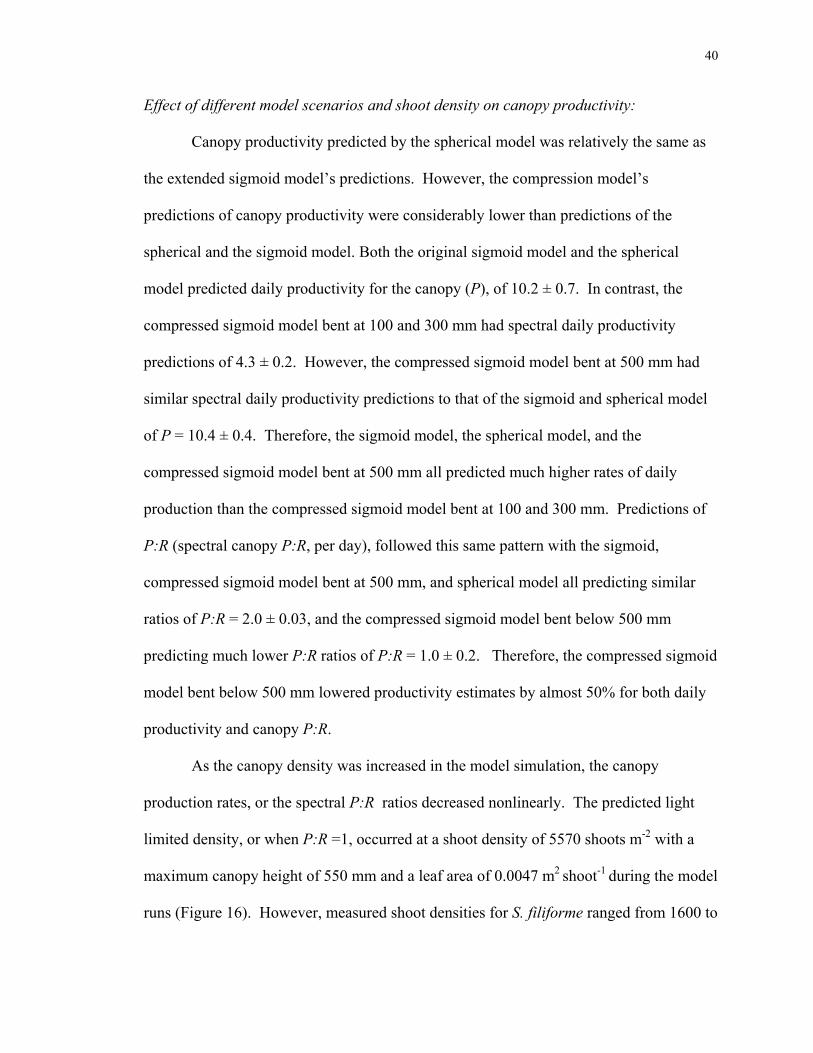
Effect of different model scenarios and shoot density on canopy productivity:

Canopy productivity predicted by the spherical model was relatively the same as

the extended sigmoid model’s predictions. However, the compression model’s

predictions of canopy productivity were considerably lower than predictions of the

spherical and the sigmoid model. Both the original sigmoid model and the spherical

model predicted daily productivity for the canopy (P), of 10.2 ± 0.7. In contrast, the

compressed sigmoid model bent at 100 and 300 mm had spectral daily productivity

predictions of 4.3 ± 0.2. However, the compressed sigmoid model bent at 500 mm had

similar spectral daily productivity predictions to that of the sigmoid and spherical model

of P = 10.4 ± 0.4. Therefore, the sigmoid model, the spherical model, and the

compressed sigmoid model bent at 500 mm all predicted much higher rates of daily

production than the compressed sigmoid model bent at 100 and 300 mm. Predictions of

P:R (spectral canopy P:R, per day), followed this same pattern with the sigmoid,

compressed sigmoid model bent at 500 mm, and spherical model all predicting similar

ratios of P:R = 2.0 ± 0.03, and the compressed sigmoid model bent below 500 mm

predicting much lower P:R ratios of P:R = 1.0 ± 0.2. Therefore, the compressed sigmoid

model bent below 500 mm lowered productivity estimates by almost 50% for both daily

productivity and canopy P:R.

As the canopy density was increased in the model simulation, the canopy

production rates, or the spectral P:R ratios decreased nonlinearly. The predicted light

limited density, or when P:R =1, occurred at a shoot density of 5570 shoots m-2 with a

maximum canopy height of 550 mm and a leaf area of 0.0047 m2 shoot-1 during the model

runs (Figure 16). However, measured shoot densities for S. filiforme ranged from 1600 to

41

2500 shoots m-2 and were well under the predicted light limitation of 5570 shoots m-2,

indicating that the meadows were not light limited (during the summer when the field

measurements were made).

Shoot Density (m2)

0 1000 2000 3000 4000 5000 6000

Dai

ly sp

ectr

al w

hole

-pla

nt P

:R

1.0

1.2

1.4

1.6

1.8

2.0Measured S. filiforme shoot densities

Figure 16. Shoot density vs daily spectral whole-plant P:R. Measured shoot densities

for Syringodium filiforme ranged from 1600-2500 shoots m-2 (grey box). Predicted light

limitation however, did not occur until the density reached 5570 shoots m-2.

42

Effects of PUR-based estimates of shoot density and optical depth:

The maximum shoot density (where P:R = 1) for all S. filiforme stations based on

PUR was strongly related to optical depth (r2PUR = 0.85). The optical depth of 2.4 is

considered to be in the mid-point of the euphotic zone, and represents 10% of the

incoming light [Ed(0)] from the surface, available for seagrasses and is commonly

recognized as the threshold for seagrass survival (Figure 17), (Duarte, 1991). Model

results suggested that the optical depth (ζ), where ζ = Kdz, was less than 2.4 for S.

filiforme, and therefore, support the commonly recognized threshold for seagrass

survival.

Optical depth (K(PAR) z)

0.6 0.8 1.0 1.2 1.4 1.6 1.8 2.0 2.2 2.4 2.6

Max

imum

Sho

ot D

ensi

ty ( P

:R=1

)

0

1000

2000

3000

4000

5000

6000

7000

PUR-based

Figure 17. Optical depth vs modeled maximum shoot density when P:R = 1 using PUR.

43

CHAPTER IV

DISCUSSION

The unique vertical biomass distribution of the S. filiforme canopy sets it apart from

other seagrass species because much of the biomass originates in the middle of the

canopy, rather than the bottom. This creates a unique biomass distribution that must be

quantified to provide the best overall description of total light absorption and scattering

by the submerged plant canopy. Although upwelling irradiances improved with the

spherical model, downwelling irradiances predicted only slightly higher % RMS values

than the original sigmoid model, indicating that the sigmoid model and spherical models

predict Ed with roughly equivalent accuracy. In fact, predictions of spectral daily

production of the entire plant canopy and P:R were similar for the original sigmoid

model, the sigmoid model compressed to 500 mm, as well as the spherical model,

suggesting that use of any of these 3 models would give accurate estimates of

productivity. However, the spherical model provides a more realistic representation of

biomass distribution of the S. filiforme canopies characterized by its undifferentiated

branching pattern. In contrast, predictions of spectral daily production and P:R, when

using the compressed model bent at heights less than 500 mm, gave about 50% lower

estimates, suggesting some sensitivity of the production estimates to canopy architecture.

The epifluorescent images of leaf cross-sections showed obvious differences in

internal leaf anatomy between the round S. filiforme leaves and the flat leaves of T.

testudinum. The chloroplasts of S. filiforme are distributed throughout the mesophyll and

epidermis, while the chloroplasts of T. testudinum are tightly packed within a single

44

epidermal layer. Photosynthetic leaf absorptance [AL (λ)] spectra for S. filiforme differed

from the [AL (λ)] for T. testudinum and Z. marina by about 40% (Cummings and

Zimmerman, 2003). The more diffuse distribution of chloroplasts throughout the leaf,

along with the higher amount of lacuanal space, significantly enhance internal scattering

within the leaf, lowering the photosynthetic absorptance and increasing the non-

photosynthetic absorptance. The high density of chloroplasts within the epidermis of T.

testudinum maximizes their exposure to light, even at the expense of the package effect,

allowing the photosynthetic absorption of T. testudinum and Z. marina to be high.

Consequently, the diffuse distribution of chloroplasts within the mesophyll and epidermal

cells of S. filiforme may reduce the package effect (increase chlorophyll light harvesting

efficiency) relative to T. testudinum and Z. marina.

The lack of an obvious green “window” in the absorption spectra also may be a

consequence of the unique structure of the S. filiforme leaf. Ramus (1978) observed

similar differences in the absorption spectra between the thallus of Ulva lactuca and the

thicker, cylindrical shaped thallus of Codium fragile, and suggested that these differences

were due to the complex internal structures in C. fragile that promote light scattering and

increase the probability of photon absorption. These findings may allow one to conclude

that S. filiforme leaves maximize their light capture due to scattering of light within their

complex internal features, particularly within their large, radialy arranged lacunae that

create unavoidable refractive boundaries that promote light scattering. This may explain

why more of the incident light is absorbed (due to non-photosynthetic tissue) when

compared to leaves of T. testudinum and Z. marina that capture light predominately due

to chlorophylls a and b (photosynthetic tissue). The package effect reduces the

45

effectiveness of light absorption by photosynthetic pigments due to the self-shading of

the chromophores between layers of chloroplasts in the leaf (Falkowski and Raven, 2007;

Cummings and Zimmerman, 2003). Increasing the absorption efficiency of S. filiforme

leaves due to multiple scattering within the tissues may counterbalance the package effect

(Enriquez, 2005). However, increased scattering within the leaf appears to reduce the

overall efficiency of photosynthetic light harvesting, and the relatively high fraction of

light absorbed by non-photosynthetic processes is not due to the package effect (which is

a measure of chlorophyll efficiency), but more likely as a result of the complex internal

structure of the S. filiforme leaf.

Unlike the absorption spectra, the reflectance spectra for S. filiforme, T.

testudinum, and Z. marina were all very similar across the visible (400-700 nm),

including the characteristic peak in the green (525-650 nm) that results from the presence

of chlorophylls a and b. The dramatic rise in reflectance in the NIR portion of the

spectrum is known as the “red edge” (enhanced near-infrared reflectance) and is due to

the presence of photosynthetic pigments absorbing the visible, but not the NIR radiation.

Also, reflectance is primarily a near-surface phenomenon, while absorption depends on

transmission through the leaf, suggesting that the complex internal structures of S.

filiforme should not influence reflectance.

Branching of S. filiforme leaves in the middle of the canopy, rather than at the

bottom, results in a biomass distribution that may also boost the canopy’s efficiency for

photosynthetic light capture used by reducing self shading and producing more evenly

illuminated leaves. This boost in light capture efficiency can be seen when the spherical

model was applied and compared to the compressed sigmoid model providing a 50%

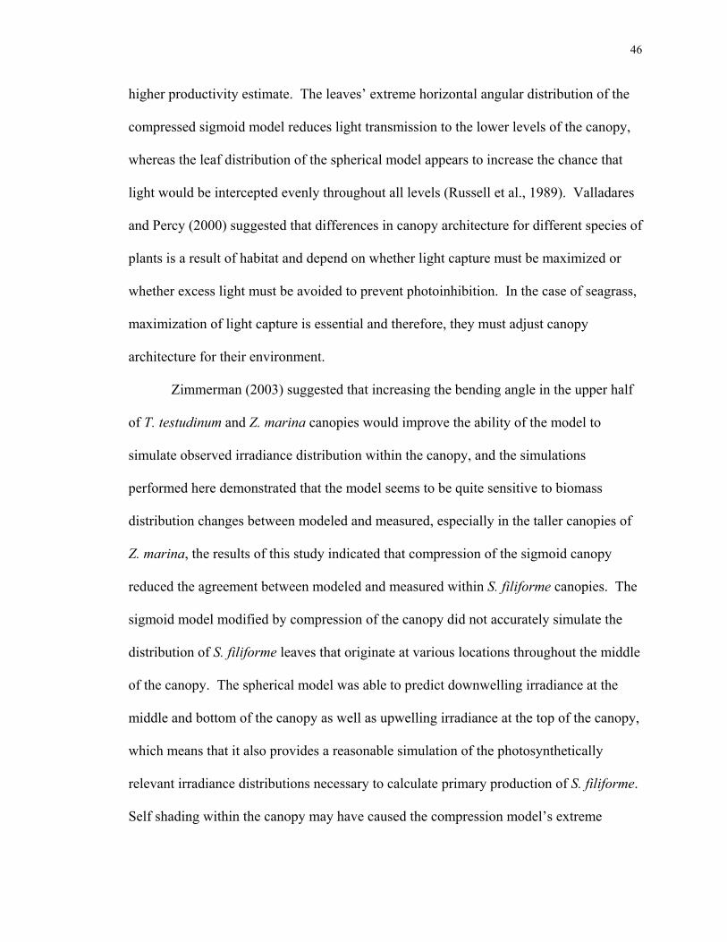
46

higher productivity estimate. The leaves’ extreme horizontal angular distribution of the

compressed sigmoid model reduces light transmission to the lower levels of the canopy,

whereas the leaf distribution of the spherical model appears to increase the chance that

light would be intercepted evenly throughout all levels (Russell et al., 1989). Valladares

and Percy (2000) suggested that differences in canopy architecture for different species of

plants is a result of habitat and depend on whether light capture must be maximized or

whether excess light must be avoided to prevent photoinhibition. In the case of seagrass,

maximization of light capture is essential and therefore, they must adjust canopy

architecture for their environment.

Zimmerman (2003) suggested that increasing the bending angle in the upper half

of T. testudinum and Z. marina canopies would improve the ability of the model to

simulate observed irradiance distribution within the canopy, and the simulations

performed here demonstrated that the model seems to be quite sensitive to biomass

distribution changes between modeled and measured, especially in the taller canopies of

Z. marina, the results of this study indicated that compression of the sigmoid canopy

reduced the agreement between modeled and measured within S. filiforme canopies. The

sigmoid model modified by compression of the canopy did not accurately simulate the

distribution of S. filiforme leaves that originate at various locations throughout the middle

of the canopy. The spherical model was able to predict downwelling irradiance at the

middle and bottom of the canopy as well as upwelling irradiance at the top of the canopy,

which means that it also provides a reasonable simulation of the photosynthetically

relevant irradiance distributions necessary to calculate primary production of S. filiforme.

Self shading within the canopy may have caused the compression model’s extreme

47

underprediction of downwelling irradiance and may have been the reason that the

compressed sigmoid model resulted in much lower productivity estimates relative to the

spherical model. Therefore, use of the spherical model can provide a robust tool for

relating photosynthetic requirements of S. filiforme to water transparency, depth

distribution and shoot density of natural populations in the field, as the sigmoid model

has been shown effective for T. testudinum and Z. marina (Zimmerman, 2003, 2006).

Incident upwelling light in all layers of the canopy (top, middle and bottom)

represented only about 3% of the total light [Eu(z) + Ed(z)] in a given layer. Therefore,

underestimation of Eu by the model had trivial impact on canopy photosynthesis that has

a measurement uncertainty of 32% (Pm = 53 ± 17 μmol O2 m2 min-1). Upwelling

irradiances at all levels in the canopy were found to be below the reported value for Ek

(Ek = 82 μmol photon m-2 sec-1) with values of 24, 14, 11 μmol m2 sec-1 at the top, middle

and bottom of the canopy respectively at noon. However, values for downwelling

irradiances were well above the reported Ek with values of 808, 678, 488 μmol m2 sec-1 at

the top, middle and bottom of the canopy, respectively at noon, indicating that at this time

during the day in the summer, S. filiforme canopies were light saturated with respect to

photosynthesis. Assuming a 12 hour day, along with applying the sun’s angle in the sky

as a sinusoidal function of time and day length, it was determined that Ed (TOC) begins

to exceed the light saturation threshold (Ek) about 22 minutes after sunrise, and drops

below Ek about 22 minutes before sunset. Thus, for 93% of the day, these S. filiforme

canopies are light saturated and are light limited only 6% of the day and also suggest that

Eu can be considered insignificant with respect to canopy photosynthesis.

48

The maximum rate of light-saturated photosynthesis exhibited by S. filiforme is

similar to that of Z. marina (Dennison and Alberte, 1985; Zimmerman et al. 1995) and T.

testudinum during the winter months (Herzka and Dunton, 1997) but only about 20% of

the summertime rate. Also, because this population of S. filiforme was found to be

operating near the theoretical limit for quantum yield (φp= 0.12) (Falkowski and Raven,

2007), the measurements used for this study could provide a reasonable upper limit

boundary for leaf optical properties that can lead to broadly accurate predictions of

maximum canopy photosynthesis in the absence of actual field measurements of specific

populations of S. filiforme.

The results also indicate that these S. filiforme populations in Florida Bay were

growing at densities (1600-2500 shoots m-2) well below light limitation (5570 shoots

m-2). However, these plants may become light limited during periods of higher turbidity

which may occur during other times of the year, such as winter and could be calculated

with the model using lower light levels and decreasing the day length.

Confidence in top of the canopy reflectance is crucial for the development of

global algorhythims for remote sensing of seagrass abundances. Predicted reflectances

for the top of the canopy (defined as Ru(λ,z) = Eu(λ,z) /Ed(λ,z)) were in good agreement

with modeled reflectance. This is crucial because there is a strong relationship between

top of the canopy reflectance and L that could be exploited for remote sensing

quantification of seagrass abundance. After correcting for the effects of the overlying

water column, the optical signature of S. filiforme or any other benthic vegetation, top of

the canopy reflectance can be retrieved and used for remote sensing purposes (Dierssen et

al., 2003; Hill et al., in prep.). However, because reflectance spectra for S. filiforme are

49

similar to that of other seagrasses, it may be difficult to distinguish different species of

seagrasses from their optical signatures alone. However, it is feasible to predict

quantitative measurements of seagrass L which, in turn, can be related to the amount of

productivity within a particular seagrass bed (Dierssen et al., 2003, Hill et al., in prep.).

50

CHAPTER V

CONCLUSION

The unique internal and external physical characteristics observed for S. filiforme,

required significant modifications of the original bio-optical model developed by

Zimmerman (2003) for T. testudinum and Z. marina. The model proved to be very

sensitive to changes in biomass distribution and bending angles within the canopy, but

not sensitive to other parameter changes such as μ , which controls the angle of

distribution of the submarine light field. This model also suggests the use of a spherical

biomass distribution within these canopies to provide a good estimate of downwelling

(throughout the entire canopy) and upwelling irradiance at the top of the canopy. This

model also provides estimates of spectral daily production as well as estimates of how

increases in L would cause S. filiforme canopies to become light limited. These results

would become useful for coastal managers to predict sudden declines in biomass due to

sudden changes in environmental conditions. A good relationship between top of the

canopy reflectance and L was determined with this model, and could become beneficial

for the remote sensing community to provide coastal managers with quantitative

measurements of seagrass abundance. Overall, understanding the biomass distribution

within any vegetative canopy and incorporating this understanding into plant bio-optical

models of light distribution and productivity, can provide essential tools for the remote

sensing, coastal and environmental communities.

51

REFERENCES

Campbell, G., and J. Norman. 1998. An introduction to environmental Biophysics.

Springer.

Campbell, J. B. 2006. Introduction to remote sensing. 4th ed. Guilford Press.

Cummings, M., and R. Zimmerman. 2003. Light harvesting and the package effect in

the seagrasses Thalassia testudinum Banks ex Konig and Zostera marina L.:

optical constraints on photoacclimation. Aquat. Bot. 75: 261-274.

Daughtry, C., K. Ranson, and L.Biehl. 1989. A new technique to measure the spectral

properties of conifer needles. Remote Sens. of Environ. 27: 81-91.

Dennison, W., R. Orth, K. Moore, J. Stevenson, V. Carter, S. Kollar, P. Bergstrom, R.

Batiuk. 1993. Assessing water quality with submerged aquatic vegetation:

habitat requirement as barometers of Chesapeake Bay health. Bio-Science. 43:

86-94.

Dennison, W., and R. Alberte. 1985. Role of daily light period in the depth distribution

of Zostera marina (eelgrass). Mar. Ecol. Prog. 25: 51-61.

Dierssen, H. M. and R.C. Zimmerman. 2003. Ocean color remote sensing of seagrass

and bathymetry in the Bahamas Banks by high-resolution airborne imagery.

Limnol. Oceanogr. 48: 444-455.

Duarte, C. M. 1991. Seagrass depth limits. Aquat. Bot. 40, no.1: 363-377.

Enriquez, S. 2005. Light absorption efficiency and the package effect in the leaves

of the seagrass Thalassia testudinum. Marine Ecology Progress Series. 289:

141-150.

52

Falkowski, P., and J. Raven, 2007. Aquatic Photosynthesis. 2nd Edition. Princeton

University Press.

Hall, M., M. Durako, J. Fourqurean, and J. Zieman. 1999. Decadal Changes in Segrass

Distribution and Abundance in Florida Bay. 22: 444-459.

Hemminga, M.A., and C. Duarte. 2000. Seagrass Ecology. Cambridge Univ. Press.

Herzka, S., and K. Dunton. 1997. Seasonal photosynthetic patterns in the seagrass

Thalassia testudinum in the western Gulf of Mexico. Mar. Ecol. Prog. Ser. 152:

103-117.

Hill, V., R. Zimmerman, P. Bissett, and H. Dierssen. In prep. Ocean color remote sensing

of seagrass meadows in Saint Josephs Bay, Florida, by hyperspectral airborne

imagery.

Hirose, T., and M. Werger. 1995. Canopy structure and photon flux partioning among

species in an herbaceous plant community. Ecology. 76: 466-474.

Kenworthy, J., and M. Fonesca. 1996. Light requirements of seagrasses Halodule

wrightii and Syringodum filiforme derived from the relationship between

diffuse light attenuation and maximum depth distribution. Estuaries. 19: 740-

750.

Kenworthy, J, and A. Schwarzschild. 1998. Vertical growth and short-shoot

demography of Syringodium filiforme in outer Florida Bay, USA. Marine

Ecology Progress Series. 173: 25-37.

Kirk, J.T.O. 1994. Light & photosynthesis in aquatic ecosystems. 2nd Edition.

Cambridege Univ. Press.

Lee, D. 1986. Unusual strategies of light absorption in rain-forest herbs. In T.J.

53

Givnish (editor), On the economy of plant form and function. Cambridge

University Press. 105-131.

Longstaff, B., and W. Dennison. 1999. Seagrass survival during pulsed turbidity

events: the effects of light deprivation on the seagrasses Halodule pinifolia and

Halophila ovalis. Aquat. Bot. 65: 105-121.

Louchard, E., R. Leathers, and T. Downes. 2003. Optical remote sensing of benthic

habitats and bathymetry in coastal environments at Lee Stocking Island,

Bahamas: A comparative spectral classification approach. 48: 511-521.

Mobley, C.D. 1994. Light and Water : Radiative Transfer in Natural Waters. Academic

Press.

Palacios, S., R. Zimmerman. 2007. Response of eelgrass Zostera marina to CO2

enrichment: possible impacts of climate change and potential for remediation of

coastal habitats. Mar. Ecol. Prog. Ser. 344: 1-13.

Ramus, J. 1978. Seaweed anatomy and photosynthetic performance: the ecological

significance of light guides, heterogeneous absorption and multiple scatter. J.

Phycol. 14: 352-362.

Russell, G., P. Jarvis, J. Monteith. 1989. Radiation absorption by canopies and stand

growth. Plant canopies: their growth, form and function. Cambridge

University Press. 21-39.

Short, F.T., S. Wyllie-Echeverria. 1996. Natural and human-induced disturbance of

seagrasses. Environ. Conserv. 23: 17-27.

Valladares, F., R. Pearcy. 2000. The role of crown architecture for light harvesting

carbon gain in extreme light environments assessed with a realistic

54

3-D model. Anales Jard. Bot. Madrid. 58: 3-16.

Verhoef,W., H. Bach. 2007. Coupled soil-leaf-canopy and atmosphere radiative

transfer modeling to simulate hyperspectral multi-angular surface reflectance

and TOA radiance data. Remote Sens. Environ. 109: 166-182.

Vermaat, J.E., N. Agawin, C. Duarte, M. Fortes, N. Marba, J. Uri. 1995. Meadow

maintenance, growth and productivity of a mixed Philippine seagrass bed.

Mar. Ecol. Prog. Ser. 124: 215-225.

Zimmerman, R.C. 2003 A biooptical model of irradiance distribution and

photosynthesis in seagrass canopies. Limnol. and Oceanogr. 48: 568-585.

Zimmerman, R.C. 1995. Eelgrass (Zostera marina L.) transplants in San Francisco

Bay: Role of light availability on metabolism, growth and survival. Aquat.

Bot. 51: 67-86.

Zimmerman, R.C. 1987. Evaluation of variance approximation techniques for non-

linear photosynthesis-irradiance models. Mar. Biol. 95: 209-215.

Zimmerman, R., D. Kohrs, D. Steller, R. Alberte. 1997. Impacts of CO2, enrichment

on productivity and light requirements of eelgrass. Plan. Physiol. 115: 599-

607.

Zimmerman, R.C. 2006. Light and photosynthesis in seagrass meadows. Seagrasses:

Biology, Ecology and Conservation. Springer.

Zimmerman, R., A. Dekker. 2006. Aquatic Optics: Basic concepts for understanding

how light affects seagrasses and makes them measurable from space.

Seagrasses: Biology, Ecology and Conservation. Springer.

55

56