› bitstream › handle › 10919 › 74533 › ld5655.v855... · an analysis of low-earth-orbit...

An Analysis of Low-Earth-Orbit

Satellite Communication Systems

by

James Henry Polaha

Thesis submitted to the Faculty of the

Virginia Polytechnic Institute and State University

in partial fulfillment of the requirements for the degree of

Master of Science

ll1

The Bradley Department of Electrical Engineering

APPROVED: A

Timothy Pratt, Chairman

Charl¥ W. Bostian u' Th~dor;-§~ Rappaport

May, 1989

Blacksburg, Virginia

An Analysis of Low-Earth-Orbit

Satellite Communication Systems

by

James Herny Polaha

Timothy Pratt, Chairman

The Bradley Department of Electrical Engineering

(ABSTRACT)

There is an ever increasing need for low-cost communication systems in the world. One such

system, low-earth-orbit satellites, can provide store-and-forward, as opposed to real time,

communication for many earth stations. The advantages and disadvantages of such a system is

presented. Material covering protocols and communications architectures is elaborated upon for

the use of amateur radio communications. Doppler shift and its effect on satellites in

low-earth-orbit is examined. Efficiency and throughput of the Amateur X.25 Protocol will be

explored. The last chapter entails the analysis of the PACSAT experiment.

Acknowledgements

I would like to acknowledge my committee, for all their help and encouragement throughout my

two-year stay at Virginia Tech. They have helped me grow in many aspects of my professional

career. I would also like to thank and , both from the Science

Applications International Corporation (SAIC), for their help over my two-month summer

employment with SAIC in 1988. Thanks also to the Defense Advanced Research Projects Agency

(DARPA), who funded the project I worked on while at SAIC. Their ideas and prodding enabled

me to complete this thesis. Without the help and encouragement of both of my parents, and

, I would never have made it this far in my college career. Thanks to all!

Acknowledgements iii

Table of Contents

1.0 Introduction . . . . . . . . . . . . . . . . . . . . . . . . . . . . . . . . . . . . . . . . . . . . . . . . . . . . . . . . 1

2.0 An Overview of Low-Earth-Orbit Satellites . . . . . . . . . . . . . . . . . . . . . . . . . . . . . . . . . . 4

'j 2.1 Satellite Orbits .......................... : . . . . . . . . . . . . . . . . . . . . . . . . . . . 4

2.1.1 Introduction . . . . . . . . . . . . . . . . . . . . . . . . . . . . . . . . . . . . . . . . . . . . . . . . . . . . . 4

2.1.2 Altitude, Inclination, and Lifetime . . . . . . . . . . . . . . . . . . . . . . . . . . . . . . . . . . . . . 9

2.1.3 Visibility . . . . . . . . . . . . . . . . . . . . . . . . . . . . . . . . . . . . . . . . . . . . . . . . . . . . . . . 11

12.2 Launches and Launch Costs . . . . . . . . . . . . . . . . . . . . . . . . . . . . . . . . . . . . . . . . . . . 13

2.2.1 Shuttle Launches . . . . . . . . . . . . . . . . . . . . . . . . . . . . . . . . . . . . . . . . . . . . . . . . 13

2.2.2 Expendable Launch Vehicles . . . . . . . . . . . . . . . . . . . . . . . . . . . . . . . . . . . . . . . . 14

2.2.3 Air Launch Vehicles . . . . . . . . . . . . . . . . . . . . . . . . . . . . . . . . . . . . . . . . . . . . . . 15

2.3 Potential Communications Uses for Low-Earth-Orbit Satellites . . . . . . . . . . . . . . . . . . 16

2.3.1 Introduction . . . . . . . . . . . . . . . . . . . . . . . . . . . . . . . . . . . . . . . . . . . . . . . . . . . . 16

2.3.2 Store-and-Forward Communications . . . . . . . . . . . . . . . . . . . . . . . . . . . . . . . . . . 17

2.3.3 Real-Time Communications . . . . . . . . . . . . . . . . . . . . . . . . . . . . . . . . . . . . . . . . 20

2.3.4 Mobile Radio . . . . . . . . . . . . . . . . . . . . . . . . . . . . . . . . . . . . . . . . . . . . . . . . . . . 22

2.3.5 Summary . . . . . . . . . . . . . . . . . . . . . . . . . . . . . . . . . . . . . . . . . . . . . . . . . . . . . . 24

Table of Contents iv

3.0 Amateur X.25 Protocol . . . . . . . . . . . . . . . . . . . . . . . . . . . . . . . . . . . . . . . . . . . . . . . 25

3.1 Protocols and Architectures . . . . . . . . . . . . . . . . . . . . . . . . . . . . . . . . . . . . . . . . . . . . 25

3.2 Open Systems Interconnection . . . . . . . . . . . . . . . . . . . . . . . . . . . . . . . . . . . . . . . . . . 26

3.3 Amateur X.25 History . . . . . . . . . . . . . . . . . . . . . . . . . . . . . . . . . . . . . . . . . . . . . . . . 28

3.4 Frame Structure . . . . . . . . . . . . . . . . . . . . . . . . . . . . . . . . . . . . . . . . . . . . . . . . . . . . 30

3.4.1 Flag Field ...................................................... 31

3.4.2 Address Field . . . . . . . . . . . . . . . . . . . . . . . . . . . . . . . . . . . . . . . . . . . . . . . . . . . 31

3.4.3 Control Field . . . . . . . . . . . . . . . . . . . . . . . . . . . . . . . . . . . . . . . . . . . . . . . . . . . 34

3.4.4 Protocol Identifier Field . . . . . . . . . . . . . . . . . . . . . . . . . . . . . . . . . . . . . . . . . . . 34

3.4.5 Information Field . . . . . . . . . . . . . . . . . . . . . . . . . . . . . . . . . . . . . . . . . . . . . . . . 34

3.4.6 Frame Check Sequence Field . . . . . . . . . . . . . . . . . . . . . . . . . . . . . . . . . . . . . . . . 36

3.5 Protocol Efficiency . . . . . . . . . . . . . . . . . . . . . . . . . . . . . . . . . . . . . . . . . . . . . . . . . . 36

3.6 Network Throughput . . . . . . . . . . . . . . . . . . . . . . . . . . . . . . . . . . . . . . . . . . . . . . . . 37

4.0 Packet-Radio . . . . . . . . . . . . . . . . . . . . . . . . . . . . . . . . . . . . . . . . . . . . . . . . . . . . . . 43

4.1 Introduction . . . . . . . . . . . . . . . . . . . . . . . . . . . . . . . . . . . . . . . . . . . . . . . . . . . . . . . 43

4.2 Early Packet-Radio Protocols . . . . . . . . . . . . . . . . . . . . . . . . . . . . . . . . . . . . . . . . . . 45

4.3 A Typical Connection . . . . . . . . . . . . . . . . . . . . . . . . . . . . . . . . . . . . . . . . . . . . . . . . 45

4.4 Applications ....................................................... 47

4.5 Earth Station Design . . . . . . . . . . . . . . . . . . . . . . . . . . . . . . . . . . . . . . . . . . . . . . . . . 48

4.5.1 Introduction . . . . . . . . . . . . . . . . . . . . . . . . . . . . . . . . . . . . . . . . . . . . . . . . . . . . 48

4.5.2 Computer . . . . . . . . . . . . . . . . . . . . . . . . . . . . . . . . . . . . . . . . . . . . . . . . . . . . . . 50

4.5.3 Terminal-Node Controller . . . . . . . . . . . . . . . . . . . . . . . . . . . . . . . . . . . . . . . . . . 50

4.5.4 Modem . . . . . . . . . . . . . . . . . . . . . . . . . . . . . . . . . . . . . . . . . . . . . . . . . . . . . . . 52

4.5.5 Transceiver . . . . . . . . . . . . . . . . . . . . . . . . . . . . . . . . . . . . . . . . . . . . . . . . . . . . . 53

4.5.6 Antenna . . . . . . . . . . . . . . . . . . . . . . . . . . . . . . . . . . . . . . . . . . . . . . . . . . . . . . . 53

4.5.7 Recommended Configuration ....................................... 55

Table of Contents v

.J 5.0 Virginia State Coverage . . . . . . . . . . . . . . . . . . . . . . . . . . . . . . . . . . . . . . . . . . . . . . . 56

5.1 Satellite Constellations . . . . . . . . . . . . . . . . . . . . . . . . . . . . . . . . . . . . . . . . . . . . . . . . 56

5.2 Statistical Analysis . . . . . . . . . . . . . . . . . . . . . . . . . . . . . . . . . . . . . . . . . . . . . . . . . . . 58

5.3 Summary . . . . . . . . . . . . . . . . . . . . . . . . . . . . . . . . . . . . . . . . . . . . . . . . . . . . . . . . . 70

6.0 Continental United States Coverage . . . . . . . . . . . . • . . . . . . . . . . . . . . . . • . . . . . . . . 71

6.1 Satellite Constellations . . . . . . . . . . . . . . . . . . . . . . . . . . . . . . . . . . . . . . . . . . . . . . . . 71

6.2 Statistical Analysis . . . . . . . . . . . . . . . . . . . . . . . . . . . . . . . . . . . . . . . . . . . . . . . . . . . 71

6.3 Summary . . . . . . . . . . . . . . . . . . . . . . . . . . . . . . . . . . . . . . . . . . . . . . . . . . . . . . . . . 74

7.0 Simulation Study of Low-Earth-Orbit Satellite Systems . . . . . . . . . . . . . . . . . . . . . . . . 85

7.1 Compressed Text ................................................... 85

7.2 Satellite Path Geometry . . . . . . . . . . . . . . . . . . . . . . . . . . . . . . . . . . . . . . . . . . . . . . . 86

7.3 Link Budget Calculations . . . . . . . . . . . . . . . . . . . . . . . . . . . . . . . . . . . . . . . . . . . . . 87

7.4 Doppler Shift Frequency . . . . . . . . . . . . . . . . . . . . . . . . . . . . . . . . . . . . . . . . . . . . . . 94

7 .4.1 Introduction . . . . . . . . . . . . . . . . . . . . . . . . . . . . . . . . . . . . . . . . . . . . . . . . . . . . 94

7.4.2 Rotation of the Earth . . . . . . . . . . . . . . . . . . . . . . . . . . . . . . . . . . . . . . . . . . . . . 97

7.4.3 Satellite Motion . . . . . . . . . . . . . . . . . . . . . . . . . . . . . . . . . . . . . . . . . . . . . . . . . 98

8.0 PACSAT Scenario . . . . . . . . . . . . . . . . . . . . . . . . . . . . . . . . . . . . . . . . . . . . . . . . . 115

8.1 Introduction . . . . . . . . . . . . . . . . . . . . . . . . . . . . . . . . . . . . . . . . . . . . . . . . . . . . . . 115

8.2 Types of Earth Stations . . . . . . . . . . . . . . . . . . . . . . . . . . . . . . . . . . . . . . . . . . . . . . 116

8.3 System Analysis . . . . . . . . . . . . . . . . . . . . . . . . . . . . . . . . . . . . . . . . . . . . . . . . . . . 117

9.0 Conclusion . . . . . . . . . . . . . . . . . . . . . . . . . . . . . . . . . . . . . . . . . . • • . . . . . . . . . . . 121

References . . . . . . . . . . . . . . . . . . . . . . . . . . . . . . . . . . . . . . . . . . . . . . . . . . . . . . . . . . . 123

Table of Contents vi

Bibliography . . . • . . . . . . . . . . . . . . . . . . . . • . . . . . . . . . . . . . . . . . . . . . . . . . . . . . . . . . 125

Appendix A. Low-Earth-Orbit Satellites in Use . . . . . . . . . . . . . . . . . . . . . . . . . . . . . . . . . 128

A.1 GLOMR . . . . . . . . . . . . . . . . . . . . . . . . . . . . . . . . . . . . . . . . . . . . . . . . . . . . . . . . 128

A.2 NUSAT

A.3 ORION

129

130

A.4 UoSAT . . . . . . . . . . . . . . . . . . . . . . . . . . . . . . . . . . . . . . . . . . . . . . . . . . . . . . . . . 131

Appendix B. Sources of Packet-Radio Information . . . . . . . . . . . . . . . . . . . . . . . . . . . . . . 134

Appendix C. Doppler Information . . . . . . . . . . . . . . . . . . . . . . . . . . . . . . . . . . . . . . . . . . 136

Appendix D. Actual lnview Times . . . . . . . . . . . . . . . . . . . . . . . . . . . . . . . . . . . . . . . . . . 145

Appendix E. Earth Station Component Specifications . . . . . . . . . . . . . . . . . . . . . . . . . . . . 166

E.1 Computer . . . . . . . . . . . . . . . . . . . . . . . . . . . . . . . . . . . . . . . . . . . . . . . . . . . . . . . 166

E.2 Terminal-Node Controller . . . . . . . . . . . . . . . . . . . . . . . . . . . . . . . . . . . . . . . . . . . . 174

E.3 Modem . . . . . . . . . . . . . . . . . . . . . . . . . . . . . . . . . . . . . . . . . . . . . . . . . . . . . . . . . 177

E.4 Transceiver and Power Supply . . . . . . . . . . . . . . . . . . . . . . . . . . . . . . . . . . . . . . . . 178

E.5 Antenna and Rotator . . . . . . . . . . . . . . . . . . . . . . . . . . . . . . . . . . . . . . . . . . . . . . . 181

Vita . . . . . . . . . . . . . . . . . . . . . . . . . . . . . . . . . . . . . . . . . . . . . . . . . . . . . . . . . . . . . . . . 185

Table of Contents vii

List of Illustrations

Figure 1. Unnumbered and supervisory frame structure of the AX.25 protocol [20] . . . . . . 32

Figure 2. Information frame structure of the AX.25 protocol [20] . . . . . . . . . . . . . . . . . . . 33

Figure 3. Address field of the AX.25 frame [20] . . . . . . . . . . . . . . . . . . . . . . . . . . . . . . . . 35

Figure 4. Minimum number of information field bytes for required throughput . . . . . . . . . 38

Figure 5. Typical packet-radio equipment . . . . . . . . . . . . . . . . . . . . . . . . . . . . . . . . . . . . 49

Figure 6. Time-averaged percent of window covered for one satellite constellation . . . . . . . 62

Figure 7. Time-averaged percent of window covered for three satellite constellation . . . . . . 63

Figure 8. Time-averaged percent of window covered for five satellite constellation . . . . . . . 64

Figure 9. Time-averaged percent of window covered for seven satellite constellation . . . . . . 65

Figure 10. Histogram for Virginia using seven satellite constellation . . . . . . . . . . . . . . . . . . 69

Figure 11. Time-averaged percent of window covered for one satellite constellation . . . . . . . 76

Figure 12. Time-averaged percent of window covered for three satellite constellation . . . . . . 77

Figure 13. Time-averaged percent of window covered for five satellite constellation . . . . . . . 78

Figure 14. Time-averaged percent of window covered for seven satellite constellation . . . . . . 79

Figure 15. Histogram for CONUS using seven satellite constellation . . . . . . . . . . . . . . . . . . 83

Figure 16. Satellite path geometry model . . . . . . . . . . . . . . . . . . . . . . . . . . . . . . . . . . . . . . 88

Figure 17. Geometry for computing contribution to worst case Doppler shift from satellite motion only (circular orbit) . . . . . . . . . . . . . . . . . . . . . . . . . . . . . . . . . . . . . . 96

Figure 18. Doppler shift for zero degree elevation angle and above . . . . . . . . . . . . . . . . . . 102

Figure 19. Doppler shift for five degree elevation angle and above 103

Figure 20. Doppler shift for ten degree elevation angle and above 104

List of Illustrations viii

Figure 21. Doppler shift for fifteen degree elevation angle and above . . . . . . . . . . . . . . . . . 105

Figure 22. Doppler shift for twenty degree elevation angle and above . . . . . . . . . . . . . . . . I 06

Figure 23. Plot of all Doppler frequencies for forty-two consecutive passes . . . . . . . . . . . . I 07

Figure 24. Histogram for all Doppler using a one satellite constellation . . . . . . . . . . . . . . . 108

Figure 25. Histogram for Doppler acquistion frequencies for five varying . . . . . . . . . . . . . 111

Figure 26. Rate of change of Doppler shift . . . . . . . . . . . . . . . . . . . . . . . . . . . . . . . . . . . 112

List of Illustrations ix

List of Tables

Table 1. Lifetime of GAS satellite versus initial altitude [15) . . . . . . . . . . . . . . . . . . . . . . . 10

Table 2. Maximum communication time for two separated earth stations . . . . . . . . . . . . . 21

Table 3. Minimum number of information field bytes for required throughput . . . . . . . . . 39

Table 4. Time (in minutes) to download memory on Hgood" link ................... 41

Table 5. Time (in minutes) to download memory on Hbad" link .................... 42

Table 6. Orbital elements for the seven satellite constellation . . . . . . . . . . . . . . . . . . . . . . 57

Table 7. Location of earth stations in the state of Virginia . . . . . . . . . . . . . . . . . . . . . . . . 61

Table 8. Minimum and maximum inview times per day . . . . . . . . . . . . . . . . . . . . . . . . . . 66

Table 9. Number of inviews and average time of inview per day . . . . . . . . . . . . . . . . . . . . 67

Table 10. Total inview times per day . . . . . . . . . . . . . . . . . . . . . . . . . . . . . . . . . . . . . . . . 68

Table 11. Location of earth stations in the continental United States . . . . . . . . . . . . . . . . . 75

Table 12. Minimum and maximum inview times per day . . . . . . . . . . . . . . . . . . . . . . . . . . 80

Table 13. Number of inviews and average time of inview per day . . . . . . . . . . . . . . . . . . . . 81

Table 14. Total inview times per day . . . . . . . . . . . . . . . . . . . . . . . . . . . . . . . . . . . . . . . . 82

Table 15. Minimum altitude for link between satellites . ........................... 89

Table 16. Doppler acquisition frequencies in hertz for a 430 MHz carrier frequency . ..... 109

Table 17. Doppler acquisition frequencies statistics . ............................ 110

Table 18. Number of seconds in restricted windows ............................. 113

Table 19. Mean, standard deviation, and variance of restricted windows . . . . . . . . . . . . . . 114

List of Tables x

1.0 Introduction

The thesis begins with a general introduction to satellites and their orbits and then discusses the

particular characteristics of low earth orbits. This is followed by a review of LEO technology and

costs. A set of appendices documents some of the LEO systems in use and the information on

LEO orbits that is available from NASA, as well as Doppler information and actual inview times.

The work described here began with the hypothesis that a network of LEO satellites in circular

orbits could be configured to provide commercially attractive store-and-forward communications

for wide area networks (WAN's), and that a constellation of such satellites in low elliptical orbits

could be configured to provide real time mobile radio support.

There are three main areas or problems that this thesis investigates. The first includes the

conceptual design of a semi-portable, low-cost earth station. The design will use amateur radio

equipment and an omnidirectional, low-gain antenna. The second area that this thesis examines

is the coverage that LEO satellites can afford for the state of Virginia and for the continental United

States. Constellations using one, three, five, and seven satellites will be analyzed. Specific earth

stations located in the state of Virginia and on the continental United States will be explored, along

with their actual inview times for a one day simulation. The final major problem is with the

Introduction

associated Doppler shifts of LEO satellites. The thesis will introduce the idea of the Doppler effect

and the magnitude and rate of change of these Doppler shifts.

This thesis investigates the following questions. What are some of the uses for LEO satellites? Is

real-time and/or store-and-forward communications possible? What type or types of protocols are

appropriate for use with LEO satellites and their associated systems? How efficient is the chosen

protocol? What is packet-radio? How is packet-radio used? How might an earth station be

designed to utilize a LEO satellite system? What type of coverage can be expected from satellite

constellations utilizing LEO satellites? How large is the Doppler shift associated with a LEO

satellite? Is this Doppler shift a problem with respect to the design of an earth station?

Its contributions are in:

• the analysis of protocol efficiency for the Amateur X.25 protocol

• the analysis of network throughput for different scenarios

• the writing of Turbo Pascal code for the simulation of LEO satellites

• the analysis of satellite constellations for coverage of the state of Virginia

• the analysis of satellite constellations for coverage of the continental United States

• the inview generation for twenty earth stations and seven LEO satellites in circular orbits

• the link budget calculations for a LEO satellite system

• the analysis of the Doppler effect for an earth station located at Blacksburg, Virginia

Chapter two contains background information for the understanding of satellite systems. There is

an emphasis placed on the topic of low-earth-orbit satellites. Included in this chapter is an overview

of launch types and costs. Reasons for the need of low-earth-orbit satellites is given towards the

end of chapter two. Chapter two of this thesis was taken from an earlier work co-authored by the

author during his thesis work [IO] and is repeated here. Parts of sections 2.3.2 to 2.3.5 were written

by Joseph P. Havlicek [10).

Introduction 2

Chapter three introduces the reader to protocols and communication models. After the history of

the amateur X.25 protocol is explained, more detailed information on the frame structure of the

AX.25 protocol is introduced.

Chapter four explains the ideas behind packet-radio as well as earth station design. This chapter

introduces the idea of packet-radio and early packet-radio protocols.

Chapter five and six provides details of satellite constellations and statistical analysis of specific

constellations.

Chapter seven has specific calculations for the scenario of the thesis. The chapter includes a section

on satellite path geometry. Link budget calculations and Doppler shift frequencies are examined

in this chapter.

Chapter eight desribes the PA CSA T scenario and explains its development. This encompasses the

background information as seen by members of the engineering team in England.

Introduction 3

2.0 An Overview of Low-Earth-Orbit Satellites

2.1 ~ate/lite ()rbits

2.1.1 Introduction

The orbit of a satellite is nominally an ellipse with the earth at one focus. The plane containing the

ellipse is called the orbital plane. The point in the orbit where the satellite is farthest from the earth

is called the apogee, and the point where the satellite is closest to the earth is called the perigee.

Altitude is the distance from the satellite to the sub satellite point on the earth. A set of six

constants, called the orbital elements, completely specifies an orbit and a satellite's position in it.

Satellites can be grouped into six orbital types. The first - and the subject of this thesis - is the

low-earth-orbit (LEO) satellite. These satellites are in orbits at altitudes of 200 to 1,000 kilometers,

and they are used for surveying earth resources, data relaying, and navigation, as well as for low-cost

store-and-forward communication systems. Examples include Defense Systems Incorporated's

Global Low Orbiting Message Relay (GLOMR) satellite, the University of Surrey's UoSATs

An Overview of Low-Earth-Orbit Satellites 4

(Orbital Satellite Carrying Amateur Radio (OSCAR) 9 and 11), and Utah State University's

Northern Utah Satellite (NUSAT). The typical orbital period for LEO satellites is approximately

90 minutes, and they have a time in line-of-sight on the order of 15 minutes. This is the maximum

time they can communicate directly with any one earth station on a single orbital pass under line

of sight conditions.

The second group comprises satellites in a MOLNYA orbit, which was first used by the Soviet

Union in the 1960's for television transmission to its remote areas and has an apogee of

approximately 40,000 kilometers and a perigee of approximately 1,000 kilometers. The MOLNYA

orbit is a highly eccentric, elliptical orbit inclined at 63.4 degrees to the equatorial plane. The

apogee is above the Northern Hemisphere. Over eighty have been launched during the past twenty

years. However, this type of orbit is not popular in the commercial world, because at least four

MOLNYA satellites are needed to provide year-round coverage at peak hours of the business day.

Communications are established when the satellite is in the apogee region where the angular

velocity of the satellite is small and antenna tracking can be slow. The satellite visibility for a station

above 60 degrees latitude with an antenna elevation greater than 20 degrees is between 4.5 and 10.5

hours. Thus, the satellite appears to remain quasi-stationary, and is useable for periods of 8 to 12

hours. Due to the motion of the satellite with respect to an observer on the earth, a sizeable

Doppler shift is associated with this orbit, and radio receivers must compensate for this. Another

MOLNY A-type orbit was used by AT &T's original TELSTAR satellites. These satellites had

typical periods of 5 to 12 hours, with a time in line of sight of 2 to 4 hours.

The third orbital type is the Apogee at Constant time-of-day Equatorial (ACE) orbit [21]. This

orbital type was developed by Ford Aerospace Corporation, under a NASA-Lewis Research Center

contract. The contract was completed in May of 1987. A single ACE orbit satellite can do the job

of several MOLNYA satellites in providing constant time-of-day coverage throughout the year.

The orbit of the ACE satellite reorients itself with respect to the sun. If the plane of the orbit lies

in the plane of the earth's equator, which the ACE orbit does, the orbit's elliptical shape will rotate

within the equatorial plane. Thus, the useful apogee region remains above a specific time zone


throughout the year. The ACE orbit has a period of one-fifth of a day or 4.8 hours, a perigee radius

of 7,410 kilometers, and an apogee radius of 21,480 kilometers. Perigee altitude is 1,030 kilometers

and apogee altitude is 15, 100 kilometers. East Coast and Midwest coverages can be optimized by

placing one of the satellite's apogee-crossings at 48 degrees West and setting the time of the crossing

to 11:50 AM EST. The next apogee occurs 4.8 hours later (4:38 PM EST) at 120 degrees West,

so both United States traffic peaks are serviced. There are however some disadvantages to the ACE

orbit. The first being that an earth station must be equipped with an antenna capable of tracking

the satellite as it moves eastward across the sky. The second disadvantage is the high radiation

environment in which the ACE satellite operates, since its orbital path carries it through the Van

Allen radiation belt's equatorial region. Thus, it is exposed to higher doses of charged particles than

other satellite orbits that would not enter the Van Allen radiation belt.

The fourth orbital type is the TUNDRA orbit. It too is a highly eccentric, elliptical orbit with an

apogee of 46,300 kilometers and a perigee of 25,250 kilometers. It exhibits characteristics very

similar to the MOLNYA orbit. Both the MOLNYA and the TUNDRA are candidates for mobile

satellite systems and for complementing geostationary coverage. The fifth orbit is the circular

geostationary orbit with an altitude of 35, 786 kilometers. The sixth orbit is the inclined circular

geosynchronous orbit [6, 13]. This provides an orbital period of 24 hours, but the satellite does not

remain stationary with respect to its earth stations as in the case with the geostationary satellite.

A satellite is subject to a variety of forces which arise from effects which are ignored in the simple

two-body analysis used to determine the equations of orbit. For example, the earth's radius varies

between the poles and the equator, and the equatorial radius varies slightly with location. These

differences are called triaxiality, and significantly affect the orbit of a satellite. The oblateness of the

earth makes the direction of the force of gravity vary with location. For example, at the equator,

the earth approximates an ellipsoid with axes at longitudes 105 degrees west and 75 degrees east.

A geostationary satellite experiences a transverse force, since the gravitational force does not act

through the center of the earth. If the transverse force is in the same direction as the satellite

motion, it increases both the height of the orbit and the orbital period. The sub-satellite point drifts


backwards towards the equilibrium point at the minor axis [6). Readers familiar with geostationary

satellites will be aware of this effect and the resulting need for stationkeeping. The amount of

stationkeeping fuel that a geostationary satellite can carry is an important limiting factor in its

lifetime.

For non-equatorial and non-polar orbits there is a gravitational component perpendicular to the

plane of the orbit which causes the orbital plane to rotate slowly about the earth's axis without

changing its inclination. This is called precession of the node. It operates in the opposite direction

to the satellite motion. The component in the plane of the orbit causes the orbital ellipse to rotate

in its own plane (nodal regression). The eccentricity of the orbit remains unchanged but the apogee

and perigee move slowly round the orbit. This effect is called apsidal rotation or precession of the

argument of perigee. LEO satellites experience nodal precession, nodal regression, and apsidal

rotation. These cause the orbit to change with time, but they have little effect on satellite lifetime.

The formula to obtain the nodal regression is [ 19)

Q=- 9.9641 ( ~£ )3.S(cosi) (1 - e2)2

(degrees per day) ( 1)

where RE is the radius of the earth, which is approximately 6,370 kilometers, e is the eccentricity

of the orbit, for a circular orbit, it is equal to zero, a is the semimajor axis length, for a circular orbit,

it is equal to the sum of the earth's radius and the satellite's altitude, and i is the inclination angle

of the satellite's orbit. The minus sign indicates that the node drifts westward for direct orbits

( i < 90°) and eastward for retrograde orbits ( i > 90°) . The nodal regression for a LEO in a circular

orbit at 800 kilometers and inclined at 82.5 degrees is 0.860 degrees per day.

The formula to obtain the apsidal rotation is (19]

(degrees per day) (2)


The apsidal rotation for a LEO in a circular orbit at 800 kilometers and inclined at 82.5 degrees is

-3.012 degrees per day.

In general, a satellite must maintain both a correct orbit (stationkeeping) and a correct orientation

(attitude). For example, the attitude control subsystem of a geostationary satellite must keep the

spacecraft's antennas and earth sensors correctly pointed towards the earth, and keep the solar cells

correctly pointed towards the sun. Due to the rotation of the earth, all attitude control systems

must pitch the satellite 15 degrees per hour to maintain earth pointing. However, the attitude

control system does not require active control once the orientation is correct. It must also correct

for disturbances due to radiation pressure and torques generated by stationkeeping maneuvers.

Most satellites use either spin stabilization or three-axis stabilization.

In the spin stabilized system (a one-axis system), the body of the spacecraft is spun with the spin

axis normal to the orbit plane. Since the high gain antennas must be pointed towards the earth it

is necessary for the antennas to be despun or counter-rotated. This can mean despinning the entire

platform containing the payload. In this type of spacecraft, the solar cells are mounted on a

cylindrical drum which forms the outer wall of the spacecraft.

In the three axis or body stabilized system, the spacecraft body usually contains one or more

momentum wheels or three reaction wheels spinning inside the spacecraft. In this configuration,

the solar cells are mounted on panels protruding from the spacecraft body. It is usual to employ

a momentum wheel to give the gyroscopic rigidity inherent in the spin stabilized satellite. Speeding

up or slowing down of the wheel produces a reaction on the satellite about the spin axis of the

wheel. Wheels at right angles or on skewed axes can be used to produce the necessary precessing

torques [6J.

Some LEO satellites (GLOMR, NUSAT) operate without stabilization. The systems used by other

LEO's are generally simpler and cheaper than those required by geostationary satellites.


2.1.2 Altitude, Inclination, and Lifetime

This section discusses the altitude and inclination of a LEO satellite's orbit and their implications

for its geographical coverage.

Altitude is the height of a satellite above the earth. It has two practical limitations. The lowest

altitude is limited by atmospheric drag to about 200 kilometers [4]. At altitudes below about 400

kilometers, large propulsion systems are required to compensate for the aerodynamic drag of

satellites requiring long orbital lifetimes. At altitudes from approximately 1,200 to 7,000 kilometers,

the Van Allen radiation belt poses a hazard [9]. Therefore, the range of possible LEO satellite

altitudes is from approximately 200 to 1,200 kilometers, and the range of commercially useful

altitudes is from about 400 to 1,200 kilometers.

Because the density of the earth's atmosphere decreases exponentially with height, the lifetime of a

LEO is a strong function of the altitude. The atmosphere's density, and thus satellite lifetime, also

vary with sunspot activity. The response of the atmosphere to thermal inputs from sunspot activity

is fast, with response times that can be less than one hour. If the heat input is subsequently

removed, the density can relax just as rapidly. For example, during some large sunspot activity in

February 1986, both the NUSAT and GLOMR spacecraft dropped on the order of 500 meters in

one day. Under normal conditions, this should have taken one week [15]. The lifetime of a GAS

(Get Away Special, see Section 2.3.1) CAN size satellite as a function of initial altitude is shown in

Table 1 on page 10.

Inclination is the angle between a satellite's orbital plane and the earth's equatorial plane.

Inclination plays a major role in determining a LEO satellite's ground track and thus its visibility

from a particular earth station. A good value for commercial systems would be 63.4 degrees. This

gives better coverage of the East Coast than either its retrograde counterpart or a sun synchronous

orbit [9].


Table I. Lifetime of GAS satellite versus initial altitude (15)

Altitude (km) Lifetime (days) 300 30 to 90 325 55 to 150 350 100 to 400 375 200 to 700 400 350 to 1000 425 600 to 2500 450 1000 to 4000

The expected lifetime, in days, of a satellite injected into orbit from the space shuttle's Get Away Special (GAS) canister, given the initial altitude of the satellite.

An Overview of Low-Earth-Orbit Satellites lO

For many types of earth observation it would be desirable to view the same surface regions

repeatedly under constant lighting conditions. If it were possible to establish an orbit whose nodal

precession matched the solar precession, then the sun-orbit plane geometry would be fixed, with

the lighting conditions at a particular latitude dependent only on the north-south movement of the

sun with the seasons. The best available way to accomplish this is to set the orbital precession rate

equal to the average solar precession rate. The sun precesses 360 degrees in one tropical year of

365.2422 days. Therefore, from equation ( 1 ), the orbital precession rate, in degrees per day, is 360 .

365.2422 = 0.9856473 = n. The sun synchronous inclination will always be greater than 90

degrees. For a LEO satellite at an altitude of 730 kilometers and in a circular orbit, the sun

synchronous inclination is 97.8795 degrees.

2.1.3 Visibility

The key variable in determining whether a satellite can communicate with an earth station is its

elevation angle; this is the angle measured vertically from local horizontal to a line joining the earth

station and the satellite. If the elevation angle is negative, the satellite is below the horizon, and the

radio path is blocked by the earth. If the elevation angle is positive and large enough to clear the

surrounding terrain (buildings, trees, hills, etc.), there is a clear line-of-sight propagation path

between the earth station and the satellite, and then the satellite is in view. The time interval when

the satellite is in view is called an inview or a window.

Propagation effects (fading and scintillation) become very pronounced at low elevation angles

because, to a first approximation, the distance that the radio signals travel in the atmosphere is

proportional to the cosecant of the elevation angle. To be useful, an inview must provide an

elevation angle greater than some minimum value, typically 5 to 10 degrees. The simulations in this

thesis will use a minimum elevation angle of l 0 degrees, unless otherwise stated.


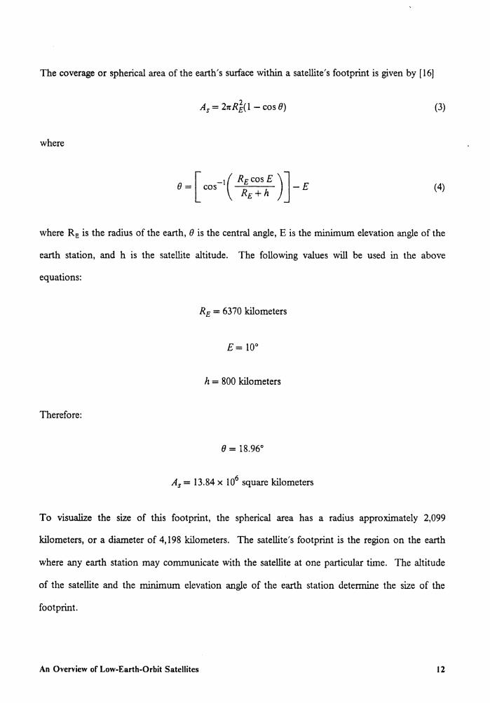
The coverage or spherical area of the earth's surface within a satellite's footprint is given by [16]

(3)

where

e = cos -E [ _ 1(REcosE)] RE+h (4)

where Ra is the radius of the earth, e is the central angle, E is the minimum elevation angle of the

earth station, and h is the satellite altitude. The following values will be used in the above

equations:

RE= 6370 kilometers

E= 10°

h = 800 kilometers

Therefore:

(J = 18.96°

A3 = 13.84 x 106 square kilometers

To visualize the size of this footprint, the spherical area has a radius approximately 2,099

kilometers, or a diameter of 4, 198 kilometers. The satellite's footprint is the region on the earth

where any earth station may communicate with the satellite at one particular time. The altitude

of the satellite and the minimum elevation angle of the earth station determine the size of the

footprint.


2.2 Launches and Launch Costs

2.2.1 Shuttle Launches

The NASA GAS (Get Away Special) program has been instrumental in developing most of the

current interest in low-cost space experiments. There are many differences between the GAS

program and other launch methods. In its original concept, the program was designed to take

advantage of the small spaces available on a large cargo system. There have been 77 GAS canisters

flown from the shuttle, some with multiple experiments aboard. The CAN SAT program allows

the launch of a satellite which is essentially a 19 inch diameter sphere from a GAS canister. The

shape of the satellite was largely driven by an early requirement that the satellite be able to rotate

within the canister without sticking. NUSAT and GLOMR were launched this way [15].

The future availability of GAS CAN launches is unknown, but posted costs are: $10,000 for a 5

cubic foot, 200 pound experiment; $5,000 for a 2.5 cubic foot, 100 pound experiment; and $3,000

for a 2.5 cubic foot, 60 pound experiment. An additional launch cost of $25,000 is for the launch

mechanism and lid replacement. These costs are for self-contained, "non-complex" experiments.

"Non-complex" implies that the experiments will not entail any extraordinary features such as the

use of on-board propulsion units.

The first commercial space shuttle launch since the Challenger disaster was the STS-29 in March

1989. GAS CAN's will be launched starting with the fourth launch, STS-32, in 1989. Four GAS

canisters are ready to be launched on that date. About 500 reservations for use of the GAS canister

are currently held. Apparently these reservations may be sold or exchanged by their holders.


2.2.2 Expendable Launch Vehicles

Following the Challenger disaster, at least two private companies entered the market and are

offering rocket launches, or expendable launch vehicles (ELY). Space Services Incorporated of

America, with facilities at Wallops Island, Virginia, is able to provide launch services within 18

months of notice. For a dedicated flight and ten percent down, they can place a 225 kilogram

satellite in a 740 kilometer polar orbit for 15 million dollars, or a 680 kilogram satellite in the same

orbit for 18 million dollars. The Conestoga series of expendable launch vehicles can place a 200

kilogram object in a 265 kilometer circular orbit, or a 860 kilogram object in a 800 kilometer orbit

[ 14).

Available performance and cost data on older EL V's predate the launch of Challenger and may be

unreliable. A summary of these are below; dollar figures are as of 1982. A Delta rocket costs

between 25 and 27 million dollars per launch. An Ariane rocket costs between 22 and 28 million

dollars per launch. The Ariane 2 is able to place a 5, 100 kilogram satellite in LEO, while Ariane

3 is able to place a 5,900 kilogram satellite in LEO. The Ariane 4 AR42L configuration is able to

place a satellite greater than 3,500 kilograms in sun synchronous orbit. The Ariane 4 AR44L

configuration is able to place a satellite greater than 4,500 kilograms in sun synchronous orbit [6).

The Atlas-Centaur is NASA's highest performance expendable launch vehicle and costs

approximately 60 million dollars per launch.

The Scout expendable launch vehicle costs between 8 and 9 million dollars and can place a 550

kilogram object in a 555 kilometer circular orbit. It can also place a 370 kilogram satellite in a 1, 110

kilometer circular orbit. Scout operational launch sites are presently established at Wallops Flight

Facility, Virginia, Vandenberg Air Force Base, California, and Ngwana Bay, Kenya, Africa [12).


2.2.3 Air Launch Vehicles

A recent concept in launch vehicles is that of air launch vehicles (ALV). In this approach a rocket

with payload is taken to high altitude aboard an aircraft and released for an air launch. The first

such launch is anticipated to be in July of 1989 using the Pegasus ALV launched from a B-52

aircraft. The Pegasus Air-Launched Space Booster developed by Orbital Sciences Corporation of

Fairfax, Virginia, and Hercules Aerospace Company of Wilmington, Delaware, is a prototype for

a new class of space satellite payloads. This technique is as yet unproven but holds great promise

for future low cost LEO satellite launches.

Pegasus is carried aloft by a conventional transport/bomber-class aircraft to level-flight launch

conditions of approximately 12,200 meters altitude and high subsonic velocity. After release from

the aircraft and ignition of its first stage motor, Pegasus follows a nearly vacuum-optimal lift-ascent

trajectory to orbit, carrying 600 pound payloads to 463 kilometers polar orbits or 900 pound

payloads to 463 kilometers equatorial orbits. Pegasus can also carry larger payloads to lower

altitude/lower inclination orbits or to suborbital trajectories. It is possible to place a 300 pound

payload into a circular orbit at an inclination of zero degrees with an altitude of 800 kilometers.

Pegasus can also place the same payload into a circular orbit at an inclination of ninety degrees at

an altitude of 600 kilometers. Pegasus was designed to be compatible with underwing launch from

several modern transport-class aircraft and from certain military aircraft.


2.3 Potential Communications Uses for Low-Earth-Orbit

Satellites

2.3.1 Introduction

Although the first communication satellites were LEOs, the inherently intermittent nature of LEO

visibility was unsuited to the analog technology of the 1960's, and geostationary satellites quickly

became the industry standard. But in the late 1980's the filling of the geostationary arc and the

rapidly growing markets for data collection and for digital and cellular radio have made LEO' s

commercially attractive.

Potential applications include [ 14, 17]:

Remote Sensing

Oil and gas well head

Oil and gas pipeline flow

Soil moisture and temperature

Electric power meter readings

Snow pack readings

Security monitors for businesses, and homes, power stations, warehouses, etc.

Effiuent monitoring

Stream flow

Reservoir levels

Traffic counts

Brief, point-to-center message collection for truck drivers, yachtsmen, hunters, hobbyists, etc.

Search and rescue communications


Vehicle location and tracking, particularly for hazardous or illegal cargo

Navigation

While a single LEO satellite can cover only a limited region of the earth at any instant, a properly

selected orbit will allow a satellite to fly over the entire globe on a regular basis. For those

applications which do not require real time service, this offers a cheap way to achieve world wide

coverage.

Besides global coverage, LEO satellites have a number of advantages over geosynchronous satellites,

primarily in the area of cost. Since it may not require strict attitude control or sophisticated station

keeping or placement in geostationary orbit, a LEO spacecraft can be cheaply made and

inexpensively launched. But, the major saving is in the earth stations, usually the most expensive

total portion of a space communications system. Because of the satellite's relative nearness to the

earth, low power transmitters with simple antennas can be employed, in contrast to the big dishes

and high power ground transmitters required for geosynchronous satellites [14J. Thus LEO satellite

systems are lower in cost both in space and on the ground.

2.3.2 Store-and-Forward Communications

Geostationary satellites are used principally as fixed-position repeaters - "bent pipes in the sky" -

amplifying incoming signals and retransmitting them back to earth. While LEO's can work in this

mode for periods of mutual visibility (the TELSTAR satellites are an example), individually or in

small constellations they are more suited to store-and-forward service in which a satellite acts as a

messenger, collecting, carrying, and delivering messages to or from the earth stations over which it

passes. This is ideally suited to packet radio networks to give just one example.

The simplest form of a store-and-forward system would consist of a single low earth orbiting

spacecraft and a number of geographically distributed earth terminals. Some or all of the terminals


may be manned, in which case their users wish to send messages to and receive messages from other

earth stations in the network. Some or all of the terminals may be unmanned; their function is to

monitor some process and report data to the satellite for distribution throughout the network. In

this application, data are read from one station (most probably remote and unattended), stored

on-board the satellite, and later transmitted back to the ground at the appropriate place. The data

could include geophysical observations, oil well data, oceanographic data, and position information,

to list just a few examples.

The disadvantages of a single LEO system are that the windows are short, windows may occur only

about six times per day for stations at widely separated longitudes, the system delay may be up to

four hours, and on-board storage is limited. The largest documented on-board memory system is

only 12 megabytes (in the ORION).

These shortcomings can be somewhat overcome when one extends the case to a system employing

multiple LEO spacecraft. The immediate consequences of such an extension are that the number

of windows and the overall system storage capacity both increase linearly with the number of

satellites in the system. Of course the system cost also rises in proportion to the number of

spacecraft. System storage capacity can also be increased by adding more memory to each

spacecraft within space, power, and heat dissipation constraints.

Of the two remaining disadvantages, little can be done to improve the short window time within

the context of low-earth orbits. The problem of long system delay times can be addressed with the

implementation of a message routing scheme, however. The obvious solution is a network which

incorporates many orbiting nodes and many terrestrial nodes, and in which the orbiting nodes are

connected. A message might be relayed from one terrestrial node to another through a path

comprising many orbiting nodes. This solution is not considered for two reasons. First, the

number of low-earth orbiting nodes required to provide spacecraft to spacecraft communication is

excessive. Secondly, the problems associated with communication between two spacecraft, both


of which are moving with respect to one another, would require substantial advances in current

technology.

A better solution involves a network in which a message travels from an originating node n1 to a

terminating node nm through a path designated [n1, n2, ••• , nm], where each n1 is a network node.

If i is odd, then n1 is a terrestrial node. If i is even, then n1 is an orbiting node. Routing

optimization algoritluns could be implemented with earth station processing, satellite on-board

processing, or a combination of both. Obviously, increased processing sophistication in either the

earth stations or the satellites will increase the system cost. How the level of routing optimization

affects system cost and system performance, and how these factors are related to the number of

nodes in the network should be subjects of further study.

To conclude this section on store-and-forward communications applications, a summary of the

systems options will be presented. In the simplest case, a system consisting of one LEO spacecraft

and many terrestrial stations could be implemented. In this system, a message would be sent from

an originating earth station to the satellite. The message would be stored by the satellite and

delivered when the receiving earth station came into view. This system would offer the advantages

of low spacecraft cost and low earth station cost. But the message capacity would be small, the

system delay could be great, and the windows would be both few in number and short in duration.

With an added outlay in spacecraft cost, a system of several LEO satellites operating independently

could be implemented. The earth station cost would not be significantly affected. The overall

system storage capacity and the frequency of windows would be increased linearly with the number

of satellites. Finally, the addition of a message routing scheme could improve the system

turnaround time with the trade-offs being increased spacecraft cost, increased earth station cost, or

both.


2.3.3 Real-Time Communications

A single-spacecraft LEO satellite system inherently precludes real time communication between

geographically distributed earth stations because the satellite footprint is small and the window is

short (typically on the order of a few minutes). To illustrate the duration of real-time

communication links, consider the following case. A satellite in a circular, LEO at an altitude of

800 kilometers has a footprint which is approximately 4, 198 kilometers in diameter. Also, the

satellite has a velocity of 7.456 kilometers per second. If two earth stations were located directly

next to each other, they can communicate, via the satellite, for a maximum of 563 seconds, or 9.383

minutes. However, most earth stations are geographically separated by a larger distance. Table 2

on page 21 indicates the maximum duration of communication if two earth stations, lying directly

on the satellite's ground track, were separated by distances indicated in the table. Since the

satellite's footprint has a diameter of 4, 198 kilometers, any two earth stations separated by more

than 4, 198 kilometers cannot communicate directly, and a store-and-forward communication

system must be implemented. The above situation is highly unlikely though, however, the

accompanying table provides an indication of just how poorly a single LEO satellite system would

perform for real time communications.

On the other hand, large constellations of LEOs can provide situations in which at least one satellite

is always in view and thus offer the potential of real time communication in a mode analogous to

cellular radio. In cellular systems the repeaters are fixed, and mobile stations are handed off from

one repeater to the next as they move out of one coverage area and into another. A network

containing a large constellation of LEO's could reverse the process: the repeaters (LEO's) move

and earth stations are handed over to a new LEO as an old one moves out of range.

The exact number of LEO satellites that are required for continuous earth coverage is estimated to

be in the 200 to 300 range. The need for highly survivable communication systems in times of

crisis, coupled with continuing technology advancements, has led to the study of packet-switched


Table 2. Maximum communication time for two separated earth stations

Distance Seconds of Minutes of (kilometers) Communication Communication

10 561.62 9.360 20 560.27 9.338 30 558.93 9.293 40 557.59 9.293 50 556.25 9.271 100 549.55 9.159 200 536.13 8.936 300 522.72 8.712 400 509.31 8.489 500 495.90 8.264 1000 428.84 7.147 2000 294.72 4.912 3000 160.60 2.677 4000 26.48 0.441

The maximum time two geographically separated earth stations can communicate given the distance of separation of the two earth stations. The satellite is at an altitude of 800 kilometers.


multiple satellite systems. Such a system consists of from a few dozen to several hundred satellites,

providing a high degree of communication redundancy over the desired coverage area. The exact

number is determined from the satellite altitude and complexity of the system [2].

2.3.4 Mobile Radio

The second stated objective of this thesis is to investigate the applicability of LEO satellites to a

mobile radio system. Such a system would be analogous to existing cellular telephone systems and

provide a user in a vehicle with voice communication with both the existing telephone system and

other vehicles. The immediate problem is that for two vehicles to communicate, they must each

be in view of an orbiting network node. Furthermore, the network must provide a real time path

between these orbiting nodes. Studies indicate that this constraint could not be easily satisfied by

spacecraft in circular low-earth orbits. The required complexity is typified by a system of 200 or

more LEO satellites configured to provide real time mobile radio service [3]. Each satellite has ten

antennas for use in communicating with fixed and mobile earth stations as well as with other

satellites. For reasons discussed above, a system such as that does not merit consideration for

mobile radio. The system is essentially the same as the store-and-forward network in which the

orbiting nodes are connected (which was discarded previously).

If one were willing to address the problems of increased signal power requirements and/or increased

complexity in antenna design, however, a network consisting of spacecraft in elliptical orbit could

be considered. With five or fewer satellites in low elliptical orbit, one could provide continuous

coverage to an area the size of several states. At any given time, every earth station in the network

would be covered by at least one satellite (and perhaps by two).

Suppose that a constellation of low elliptical orbiting satellites were in place. At any given time,

the network nodes would be some large number of vehicles (mobile earth nodes) within the area


of network coverage, one or two satellites (orbiting nodes) whose footprints at that instant include

the entire area of network coverage, and some number of central controlling terrestrial stations

(fixed earth nodes). The number of fixed earth nodes would be chosen such that at any given time,

any orbiting node which is an active member of the network is within view of at least one fixed

earth node.

The problem of spacecraft to spacecraft communication has now been circumvented. Assume that

each fixed earth node is connected to the existing telephone system. Then for the mobile radio

system to be commercially attractive, it must continuously offer:

1. A real time link from any mobile earth node to some fixed earth node.

2. A real time link from some fixed earth node to any mobile earth node.

3. A real time link from any mobile earth node to any other mobile earth node.

4. A network coverage area significantly larger than that offered by existing cellular radio systems.

5. Toll rates comparable to those offered by existing cellular radio systems.

The condition in 4 is easily satisfied by a constellation of satellites in elliptical orbits. The condition

in 5 can not be addressed without further study. It seems plausible that conditions 1-3 can be

satisfied by specifying some network topology and employing a packet switching scheme. The

network has the ability at all times to connect each mobile earth node to at least one orbiting node,

each orbiting node to at least one fixed earth node, and each fixed earth node to the telephone

system. Then if the network connectivity is appropriately specified, a real time communication

system should be realizable. Preliminary investigations indicate that one problem with such a

system would be phase disparities arising from the condition that two orbiting nodes both transmit

a message directed toward a mobile earth node that is simultaneously covered by both. In any

event, the immediate goal of a study should be to investigate possible connectivities that could

satisfy the conditions in 1-3 above. To conclude this section on the application of LEO orbiting

satellites to mobile radio, it seems plausible that a commercially viable network could be

constructed if the satellites were allowed to assume elliptical orbits.


2.3.5 Summary

Assuming that one were interested in store-and-forward communication for remote process

monitoring, or any of the other applications enumerated above, why might one choose to

implement a LEO satellite system? The primary reason is cost. The literature indicates that the

total outlay for a LEO spacecraft system is typically less than one million dollars from system

inception through deployment. A primary drawback of geostationary satellite systems is the high

cost of earth terminals. Terminals for LEO satellites typically cost on the order of a few thousand

dollars. The terminals are usually small and easily moved. From this standpoint, the owner of a

LEO system could expect to sell network services to a large market of businesses who, for economic

reasons, are unable to invest in geostationary based space communications. The prospect of

investing $10,000 in sensor equipment and an earth terminal is attractive when compared to the cost

of maintaining a manned station for process monitoring, especially in locations characterized by a

hostile environment. Of course, the network owner also benefits from the low cost of the satellite

and earth terminals for the owner's own use.


3.0 Amateur X.25 Protocol

3.1 Protocols and Architectures

A protocol is used for communication between entities in different systems. Examples of entities

are user application programs, file transfer packages, data-base management systems, electronic mail

facilities, and terminals. Examples of systems are computers, terminals, and remote sensors. In

general, an entity is anything capable of sending or receiving information, and a system is a

physically distinct object that contains one or more entities. For two entities to communicate

successfully, they must know the same '1anguageH. What 1s communicated, how it is

communicated, and when it is communicated must conform to some mutually acceptable

conventions between the entities involved. The conventions are referred to as a protocol, which

may be defined as a set of rules governing the exchange of data between two entities. The key

elements of a protocol are:

• Syntax - includes such things as data format and signal levels

• Semantics - includes control information for coordination and error handling

• Timing - includes speed matching and sequencing

Amateur X.25 Protocol 25

Examples of some very similar bit-oriented protocols are:

• High-level data link control (HDLC) - developed by the International Organization for

Standardization (ISO)

• Advanced data communication control procedures (ADCCP) - developed by the American

National Standards Institute (ANSI)

• Link access procedure, balanced (LAP-B) - adopted by the International Telegraph and

Telephone Consultative Committee (CCITT) as part of its X.25 packet-switched network

standard

• Synchronous data link control (SDLC) - used by IBM (this is not a standard, but is in

widespread use)

3.2 Open Systems Interconnection

The International Organization for Standardization (ISO) plays the key role in the evolution of the

open systems interconnection (OSI) communications architecture model. One of the ISO's

technical committees (TC97) is concerned with information systems. This committee developed

the OSI model and is developing protocol standards at various layers of the model.

A widely accepted structuring technique, and the one chosen by ISO, is layering. The

communications functions are partitioned into a vertical set of layers. Each layer performs a related

subset of the functions required to communicate with another system. It relies on the next lower

layer to perform more primitive functions and to conceal the details of those functions. The lower

layer provides services to the next higher layer. Ideally, the layers should be defined so that changes

in one layer do not require changes in the other layers. The OSI reference model has seven layers.

The seven layers are:


• Level l: The Physical Layer

The physical layer is concerned with the transmission of unstructured bit streams over the

physical medium and it also deals with the mechanical, electrical, functional, and

procedural characteristics to access the physical medium.

• Level 2: The Link Layer

The link layer provides for the reliable transfer of information across the physical link and

it also sends blocks of data (frames) with the necessary synchronization, error control, and

flow control.

• Level 3: The Network Layer

The network layer provides upper layers with independence from the data transmission and

switching technologies used to connect systems and it also is responsible for establishing,

maintaining, and terminating connections.

• Level 4: The Transport Layer

The transport layer provides reliable, transparent transfer of data between end points and

it also provides end-to-end error recovery and flow control.

• Level 5: The Session Layer

The session layer provides the control structure for communication between applications

and it also establishes, manages, and terminates connections (sessions) between cooperating

applications.

• Level 6: The Presentation Layer

The presentation layer provides independence to the application processes from differences

in data representation (syntax).

• Level 7: The Application Layer

The application layer provides access to the OSI environment for users and it also provides

distributed information services.

The physical layer covers the physical interface between devices and the rules by which bits are

passed from one to another. The physical layer has four important characteristics: mechanical,


electrical, functional, and procedural. Examples of standards at this layer are RS-232-C, RS-449,

RS-422A, RS-423-A, and X.21.

The link layer attempts to make the physical layer reliable and provides the means to activate,

maintain, and deactivate the link. The principle service provided by the link layer to the higher

layers is that of error detection and control. Thus, with a fully functional link layer protocol, the

next higher layer may assume virtually error-free transmission over the link.

3.3 Amateur X.25 History

Over the years there have been several link-layer protocols suggested for amateur packet radio. The

first link-layer protocol to achieve widespread use in the amateur field was created by Douglas

Lockhart of the Vancouver (BC) Amateur Digital Communications Group (VADCG). It was

based on the IBM SDLC protocol and implemented on a packet-radio controller board designed

and built by V ADCG [ 1 ]. This protocol was used for the first few years of amateur packet-radio

activity. One of the limitations of the VADCG protocol was that it used eight bits (one byte) for

the station address. This restricted the number of stations to 255 or less, depending on how the

addressing scheme was implemented. It also required that someone had· to assign these arbitrary

addresses to each amateur in a local area.

In early 1982, the Amateur Radio Research .and Development Corporation (AMRAD) began a

study of the link-layer protocols in commercial use at the time. The intent was to recommend a

protocol that would not suffer from major limitations in a few years. The result of this study was

a recommendation for the use of a slightly modified version of the CCITT X.25 LAP-B.


In June of 1982, a series of meetings was held by AMRAD and the Radio Amateur

Telecommunications Society (RATS) of New Jersey. An exploratory meeting was held at Bell

Laboratories. Two definitive meetings in which the prototype of AX.25 protocol was developed

took place in Vienna, Virginia. Both link- and network-layer protocols were defined at that time.

Since both layers were based on the CCITT X.25 recommendation, it was <;iecided to follow the

pattern set by AT&T (BX.25 for Bell X.25) and call this new protocol AX.25, for Amateur X.25.

The link-layer protocol was then documented and circulated to other packet-radio experimenters

for comment. The network-layer proposal was held for further study.

The next step in the evolution of AX.25 was taken in October of 1982. Thomas Clark, president

of The Radio Amateur Satellite Corporation (AMSAT), hosted a gathering of most of the leaders

in amateur packet-radio at that time. AMRAD, AMSAT, the ARRL Ad Hoc Committee on

Amateur Radio Digital Communication, Pacific Packet Radio Society (PPRS), St. Louis Amateur

Packet Radio (SLAPR), and Tucson Amateur Packet Radio Corporation (TAPR) were

represented. The AMRAD version 1.1 AX.25 link-layer protocol was slightly modified and

adopted at this meeting [ l].

The first public release of the AX.25 link-layer protocol was in a paper given at the Second Amateur

Radio Computer Networking Conference, in March of 1983. Some corrections and changes have

been made since then by the ARRL Ad Hoc Committee on Amateur Radio Digital

Communications. In July of 1983, West Coast packet groups met to form WESTNET. The

WESTNET group decided to extend the AX.25 link-layer address field to accommodate up to eight

repeaters. This modification was accepted by the ARRL Committee at their November, 1983

meeting in Washington, DC. Unresolved at that meeting was the handling of the poll/final bit.

The poll/final bit is used in all types of frames. The poll/final bit is used in a command (poll) mode

to request an immediate reply to a frame. The reply to this poll is indicated by setting the response

(final) bit in the appropriate frame. Only one outstanding poll condition per direction is allowed

at a time.


When the Committee met again at Trenton, New Jersey, in April of 1984, a solution was proposed

to the poll/final bit problem. The Committee approved of a link-layer protocol on October 26,

1984. This protocol follows the CCITT X.25 Recommendation, with the exception of an extended

address field and the addition of the Unnumbered Information (UI) frame. This protocol will work

equally well in either half- or full-duplex amateur radio environments.

3.4 Frame Structure

The following discussion concerns level two of the AX.25 protocol. Link-layer packet-radio

transmissions are sent in small blocks of data, called frames. Each frame is made up of several

smaller groups, called fields. Figure 1 on page 32 shows the Unnumbered (U) and Supervisory (S)

frame structure. Figure 2 on page 33 shows the Information (I) frame structure [8].

There are six types of Unnumbered frames. The Set Asynchronous Balanced Mode (SABM)

unnumbered frame initiates a connection between two packet stations. The Disconnect (DISC)

frame terminates a connection between two packet stations. The receipt and acceptance of an

SABM or DISC frame is acknowledged by the Unnumbered Acknowledge (UA) frame. The

rejection of an SABM frame is indicated by the Disconnected Mode (DM) frame. The Frame

Reject (FRMR) frame indicates that the source station is unable to process a frame and that the

error is such that resending the frame will not correct the problem. The Unnumbered Information

(UI) frame allows data to be transmitted from a source station without a connection to the

destination source.

There are three types of Supervisory frames. The Receive Not Ready (RNR) frame indicates that

the destination station is not able to accept any more I frames because of a temporary busy

condition. The Receive Ready (RR) frame indicates that the destination station is able to receive


more I frames. The Reject (REJ) frame is used by the destination station to request a

retransmission when an out-of-sequence frame is received.

3.4.1 Flag Field

The flag field is one byte long. It occurs at both the beginning and end of each frame. A flag

consists of a zero followed by six ones followed by another zero, or 01111110. As a result of bit

stuffing, this sequence is not allowed to occur anywhere else inside a complete frame.

3.4.2 Address Field

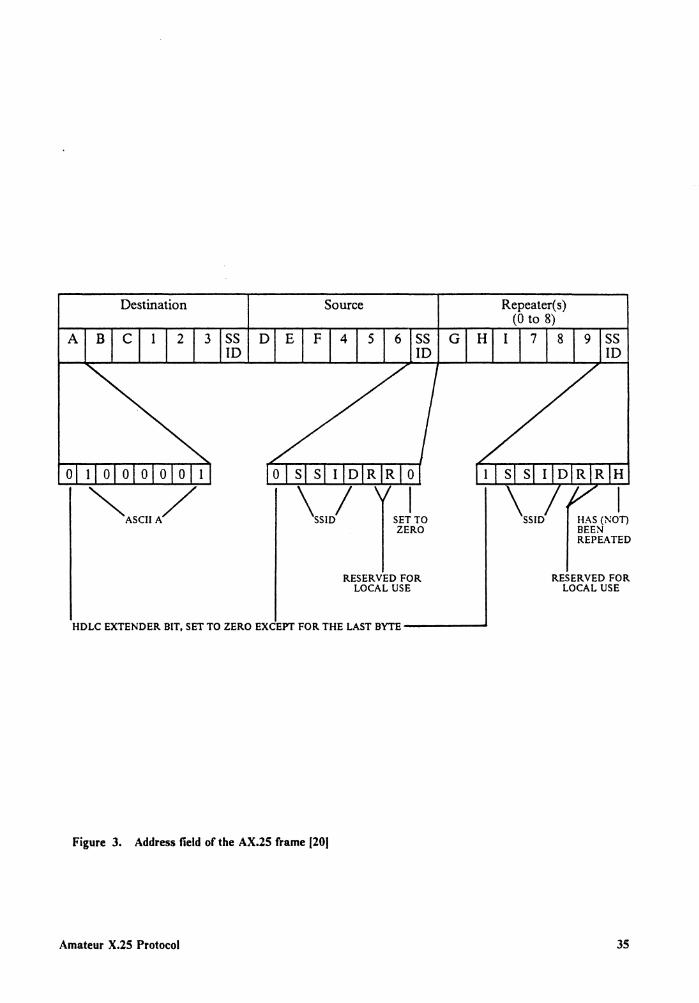
The address field can be 14 to 70 bytes long. Figure 3 on page 35 shows a typical address field and

how it is divided. The address field is used to identify both the source of the frame and its

destination. The address field contains the command/response information and facilities for level

two repeater operation.

The address field of all frames shall be encoded with both the destination and source amateur

callsigns for the frame. In Figure 3 on page 35, these are ABC123 for the destination address,

DEF456 for the source address, and GHl789 for the repeater(s) being used. Except for the

Secondary Station Identifier (SSID), the address field should be made up of upper-case alphabetic

and numeric characters only. If level two amateur repeaters are to be used, their call signs shall also

be in the address field. The HDLC address field is extended beyond one byte by assigning the

least-significant bit of each byte to be an extension bit. The extension bit of each byte is set to zero,

to indicate the next byte contains more address information, or one, to indicate this is the last byte

of the HD LC address field.


Flag Address Control Frame Check Flag Sequence

I byte 14-70 bytes I byte 2 bytes I byte

Figure 1. Unnumbered and supervisory frame structure of the AX.25 protocol (20)


Flag Address Control Protocol Information Frame Check Flag Identifier Sequence

l byte 14-70 bytes l byte l byte N bytes 2 bytes l byte

Figure 2. Information frame structure of the AX.25 protocol (201


If there are no level two repeaters being used, the address field will be 14 bytes long; however, if

repeaters are being used, the address field can be up to 70 bytes long. The destination and source

subaddresses are seven bytes long each. The destination subaddress is sent first, followed by the

source address.

There is a byte at the end of each subfield that contains the SSIO. The SSIO subfield allows an

amateur radio operator to have more than one packet-radio station operating under the same

callsign. This is useful when an amateur wants to operate a repeater as well as a regular station.

3.4.3 Control Field

The control field is one byte long. The control field is used to identify the type of frame being

passed and control several attributes of the level two connection.

3.4.4 Protocol Identifier Field

The protocol identifier (PIO) field is one byte long. The PIO field appears only in information

frames. It identifies what kind of layer three protocol is in use, if any.

3.4.5 Information Field

The information field can be up to 255 bytes long, and shall contain an integral number of bytes.

The information field is used to covey user data from one end of the link to the other. Information

fields are allowed in only three types of frames: the I frame, the UI frame, and the FRMR frame.


Destination Source Repeater(s) (0 to 8)

A SS ID

SS G H I 7 8 SS ID

0

ID

SET TO ZERO

RESERVED FOR LOCAL USE

HDLC EXTENDER BIT, SET TO ZERO EXCEPT FOR THE LAST BYTE-----

Figure 3. Address field of the AX.25 frame (201

Amateur X.25 Protocol

SSID

H

HAS (NOT) BEEN REPEATED

RESERVED FOR LOCAL USE

35

3.4.6 Frame Check Sequence Field

The frame check sequence (FCS) field is two bytes long. The FCS field is calculated by both the

sender and the receiver of a frame. It is used to insure that the frame was not corrupted by the

medium used to get the frame from the sender to the receiver. It is calculated in accordance with

ISO 3309 (HDLC) Recommendations.

3.5 Protocol Efficiency

The throughput of an AX.25 information frame is shown in Figure 4 on page 38. Overhead

includes: the flag field, the address field, the control field, the protocol identifier field, and the frame

check sequence field. The plot represents the following formula:

hr _ ( information packet length ) t oughput - information packet length + overhead (5)

The top solid line represents an information frame with no repeaters. The next line, a broken line,

represents an information frame with one repeater, etc. The bottom broken line represents an

information frame with eight repeaters. Table 3 on page 39 is a numerical representation of

Figure 4 on page 38. The numbers within the matrix of Table 3 on page 39 represent the

minimum number of information field bytes, with a given number of repeaters, necessary to obtain

the shown throughput efficiency. The third column of the accompanying table, with the column

heading 1 Number of Repeaters, represents the scenario of a single LEO satellite and multiple earth

stations. Since there will be only one repeater (the satellite), this column is of prime concern in this

investigation. The maximum throughput efficiency for the AX.25 information frame is 92.75%.

This value results since, at most, the Information field can have 255 bytes of information. The


overhead (with no repeaters) is 20 bytes long. Therefore, using equation (5), the throughput is

92.75%.

3.6 Network Throughput

Bit rates under investigation are 1200, 2400, 4800, and 9600 bits per second (bps). Memory sizes

of 1, 2, 4, 6, 8, and 10 megabytes are also being investigated for possible use. What bit rate is

required to transfer the satellite's memory?

A qualitative but limited answer to this question can be provided by looking at some of the "best"

and "worst" cases of network configuration. Remember that these answers are limited; there are

two ways of getting more accurate answers: simulation and in-orbit tests. If it was desired to dump

the entire spacecraft memory to a single station, how long would it take?

The first assumption is that there is a link where 95% of all packets are correctly received the first

time, and all frames contain 255 data bytes and 20 AX.25 header bytes. The 95% first-time-good

figure is realized on a link with 2.5 x 10-5 Bit Error Rate (BER), and results in frame throughput

of 95% [22). The 20 bytes of AX.25 header in each frame cause an 8% reduction in throughput.

The overall link efficiency is:

0.95 x 0.92 = 87% (6)

To transfer 1 megabyte, it requires:

( 1 megabyte x 1048576 byt:s x 8 bits ) mega ytes byte ( 1 · t )

x 60 rrunu; = 133.92 minutes ( 1200 bits d x 0.87 efficiency factor) secon s

secon

(7)


100

90

80 -~ 70 u

(,I

"" u 1:1. -!=I 60 0 ;I Id

~ 50 i .... 0

-a 40 1:1.

,Q : 30 0

~ 20

1 0

0

0 100

---------Zero Repeaters ·•••••••••••••••••••••••••• •· One Repeater ·------------------·Two Repeaters ------------Three Repeaters -------Four Repeaters ------Five Repeaters

Six Repeaters -·-·-·-·-·---·-··Seven Repeaters -·-·-·-·-·-Eight Repeaters

200 300

Information Field Length (bytes)

Figure 4. Minimum number of information field bytes for required throughput

Amateur X.25 Protocol

400

38

Table 3. Minimum number of information field bytes for required throughput

Number of Repeaters Through-

put 0 1 2 3 4 5 6 7 8 (percent)

10 3 3 4 5 6 7 7 8 9 20 5 7 9 11 12 14 16 18 19 30 9 12 15 18 21 24 27 30 33 40 14 18 23 28 32 37 42 46 51 50 20 27 34 41 48 55 62 69 76 60 30 41 51 62 72 83 93 104 114 70 47 63 80 96 112 129 145 161 178 80 80 108 136 164 192 220 248 276 304 90 180 243 306 369 432 495 558 621 684

The minimum number of information field data bytes required to obtain a specific throughput percentage, given the number of repeaters.


That is on a "good" link. The benchmark "bad link" was calculated such that by the fourth retry,

99% of all packets are correctly received. This is equivalent to a BER of 4.0 x 10-4, and results in

32% frame throughput [22]. Again, the factor of 8% reduction caused by AX.25 frame overhead

must be included. The overall link efficiency is:

0.32 x 0.92 = 29% (8)

To transfer 1 megabyte, it requires:

( bytes bits ) 1 megabyte x 1048576 b x 8-b-mega )1es yte

( bits ffi . c ) 1200 d x 0.29 e 1c1ency iactor secon

( 1 minute ) . x 60 d = 401.75 minutes secon s (9)

Table 4 on page 41 has different combinations of memory sizes and link bit rates to demonstrate

how many minutes would be required to download the specific memory capacity on a "good" link.

Table 5 on page 42 has different combinations of memory sizes and link bit rates to demonstrate

how many minutes would be required to download the specific memory capacity on a ''bad" link.

For example, with a link utilizing a 9600 bit rate and a four megabyte satellite memory capacity,

it would require 67 minutes to download the entire memory on a "good" link. On the "bad" link,

however, the same case would require 201 minutes. Since a single pass from a LEO satellite is

typically on the order of 15 minutes, it would require 5 passes to download the memory on a "good"

link, and 14 passes on a ''bad" link. This number of passes is quite large, considering that other

earth stations will be trying to upload their messages to the satellite while the satellite still has other

information that it must download. If the satellite's memory remains full, no new messages can

be transferred. In this case, a priority system should be implemented for messages on the satellite.

A higher priority message then can be loaded onto the satellite, while a lower priority message

would be deleted. There might also be a date associated with each message, and if the message has

expired, it would automatically be deleted from the system.


Table 4. Time (in minutes) to download memory on "good" link

Memory Bit Rate (bits per second) (megabytes) 1200 2400 4800 9600

l 133.92 66.96 33.48 16.74 2 267.83 133.92 66.96 33.48 4 535.67 267.83 133.92 66.96 6 803.51 401.75 200.88 100.44 8 1071.34 535.67 267.83 133.92 10 1339.18 819.59 334.79 167.40

Given the bit rate and the amount of memory required to transfer, the time necessary to download the entire memory on a link with a bit error rate of 2.5 x 10-s is shown.


Table S. Time (in minutes) to download memory on Hbad" link

Memory Bit Rate (bits per second) (megabytes) 1200 2400 4800 9600

1 401.75 200.88 100.44 50.22 2 803.61 401.75 200.88 100.44 4 1607.01 803.51 401.75 200.88 6 2410.52 1205.26 602.63 301.32 8 3214.03 1607.01 803.51 401.75 to 4017.53 2008.77 1004.38 502.19

Given the bit rate and the amount of memory required to transfer, the time necessary to download the entire memory on a link with a bit error rate of 4.0 x IQ-4 is shown.


4.0 Packet-Radio

4.1 Introduction

Packet-radio is a mode of digital communications. With packet-radio techniques, data are sent

from one station to another in bursts, or frames. In addition to carrying data, each of these frames

contains addressing information, error-checking information, and control information [ 11 ].

Packet-radio can provide error-free communications. With packet-radio, no time is wasted trying

to decipher communications that contain "hits" or "misses" caused by electrical interference in

propagation. Packet-radio uses the radio spectrum efficiently. One radio frequency can support

many packet-radio users. Packet-radio uses other stations efficiently. Any packet-radio station can

command other packet-radio stations to create a network for the. transfer of information.

Packet-radio uses time efficiently. Amateur radio bulletin-board systems shift time by permitting

packet-radio operators to store messages for retrieval by others at a later time.

Store-and-forward packet-switching techniques date back to a 1964 study by the RAND

Corporation. The term packet was coined in 1965 by D. W. Davies of the British National Physical

Packet-Radio 43

Laboratory. Amateur packet-radio experimentation began in Canada. Dr. John deMercado, the

Director General of Telecommunications Regulations in Canada, was responsible for combining

amateur radio and packet. It was Dr. deMercado and the Canadian Department of

Communications (DOC) who encouraged Canadian amateur radio operators to experiment with

packet-radio even before the DOC officially permitted it as an amateur communications mode.

As a result, amateur packet-radio experiments began in 1978 with the first amateur packets being

transmitted and received without error at a meeting of the Montreal Amateur Radio Club in May

of 1978.

The usual amateur frequency bands allowed by the Federal Communications Commission (FCC)

in the United States for amateur packet-radio transmissions are 145.010 to 145.090 megahertz

(MHz) and 430.05 to 430.95 MHz. The 145 MHz range utilizes a 20 kilohertz (kHz) bandwidth,

while the 430 MHz range uses a 100 kHz bandwidth. In discussing packet-radio in this thesis, the

frequency of 145 MHz will be assumed for up transmissions and 430 MHz for down transmissions

in a satellite link. Amateurs also use "High Frequency (HF) gateways", at 14.080 MHz and 7.080

MHz, to transmit packet radio data throughout the world.

One reason why Very High Frequency (VHF) and Ultra High Frequency (UHF) packet-radio is

more popular than HF packet is that higher data rates are permitted in the VHF and UHF

spectrum. Below 28 MHz, the maximum permissible data rate is 300 bps. Above 28 MHz, the

legal limit starts at 1,200 bps and increases as the operating frequency increases. The maximum

data rate is 1,200 bps between 28 MHz and 50 MHz, 19,600 bps between 50 MHz and 220 MHz,

and 56,000 bps above 220 MHz. Although some amateurs are experimenting with 4,800 and 9,600

bps data rates, the most popular data rate currently in use in the VHF and UHF spectrum is 1,200

bps.

Packet-Radio 44

4.2 Early Packet-Radio Protocols

There are basically two ways of handling packet communications. One is to have a master-control

station acting much like a net-control station in traditional amateur practice. The other is to have

all stations equal, as in casual amateur operation. The first system was developed in which a

master-control station would poll each station in its list and each station would in turn pass along

any traffic. The advantages are apparent: everyone takes his turn and any potential conflicts in

using the frequency are thereby resolved. The disadvantages are more subtle: how does one get

on the list, and what happens if the list is long but only two or three stations are active? Do the

few active users have to wait for the inactive stations to be interrogated by the master station

between every transmission? Another system was developed in which each station had its own

identification and could attempt !o access the channel at will. The possibility of a collision became

real with this system, but communications were somewhat more robust because a central controller

was not needed. There was also no need to get on the list.

The polling system is used in very few active packet areas now, and a variation of the second system

became the accepted standard. Developed by the Vancouver Amateur Digital Communications

Group, the Vancouver protocol spread with the V ADCG tenninal-node controller (TNC). Nearly

all early work with packet-radio in the United States was based on this TNC and protocol.

4.3 A Typical Connection

To illustrate the function of packet protocol, an example of a typical connection sequence follows.

Let's say that DEF456 wishes to connect to station ABC123. DEF456 would type at his tenninal

C ABC123

Packet-Radio 45

A packet would be sent that could be represented as

: FLAG : ABC123 : DEF456 : SABM : FCS : FLAG :

Note that the destination station callsign precedes the sending station callsign. Assuming ABC123

is on frequency and his TNC is allowed to accept a connection request, his station would respond

: FLAG : DEF456 : ABC123 : UA : FCS : FLAG :

In this case, the callsigns are reversed and the UA is sent in the control field to ACK the connect

request. At ABC123's terminal, the following message would be displayed

*"'*CONNECTED WITH DEF456

while DEF456 terminal would display

+++CONNECTED WITH ABC123

At this point the TN Cs would enter the conversation mode. Now any information entered at either

station will be transmitted to the other station. When the session ends, one station, say DEF456,

will place his TNC in the command mode and enter

D ABC123

at which point his TNC would send out a packet like

: FLAG : ABC123 : DEF456 : DISC : FCS : FLAG

where DISC is the control code to disconnect, and ABC123's TNC would respond

: FLAG : DEF456 : ABC123 : UA : FCS : FLAG :

and each terminal would then display

+++DISCONNECTED

While in the connect mode, any information entered at one station's TNC will be sent to the other

station and positive acknowledgement utilized to ensure that the receiving station in fact received

the frame correctly. If the receiving station does not send the required Acknowledge (ACK), the

sender will repeat it.

Packet-Radio 46

4.4 Applications

Apart from the FCC-mandated "advancement of the state of the radio art", packet provides

opportunities for experimentation and public service. Consider the aftermath of a tornado,

earthquake, volcano, or other disaster. Usually, the first emergency traffic to be handled is done

via amateur radio, especially if the damage is severe enough to knock out commercial lines of

communication. In many cases, the traffic entered into the communications system far exceeds the

ability of the system to handle it. The network becomes saturated and delays increase. It may take

hours or even days to get all the messages handled. Typically, voice or CW traffic nets are limited

to a realistic rate on the order of tens of words per minute. Fatigued operators are subject to errors

in copying and otherwise handling the information. Radioteletype (RTTY) or American National

Standard Code for Information Interchange (ASCII) offers some improvement in system capacity,

but errors are still likely. On the other hand, packet offers the capability for operators to enter

traffic without having to listen first and allows error-free communications to occur on a channel at

rates of nearly 1200 to 9600 words per minute. Multiple messages can be on the link at any given

time, and the TNCs can sort it all out. Since the TNC is likely to be coupled with a computer

system, traffic can be passed to commercial lanes as they become available. Automatic logging of

third-party traffic becomes trivial. The packet system is on the order of twenty times more efficient

than that of R TTY. The capacity is even greater compared to CW of voice nets, especially when

operator fatigue is considered.

As another example, consider the computer-minded amateur. Perhaps he has developed a program

he wishes to share with another amateur. He can place his TNC in transparent mode, where it

passes all data offered it, and send a binary file dump to the other amateur, who passes it directly

to his computer. Errors are trapped before the data are passed through, so the recipient can be sure

that if he receives the program, it is error-free.

Packet-Radio 47

Another system used extensively on packet is the bulletin board, or computerized mailbox system.

Amateurs may leave messages for other amateurs or get general information items.

4.5 Earth Station Design

4.5.1 Introduction

This section contains general information concerning the five major sections in the design of an

earth station for packet-radio use. The five major section of an earth station are:

• Computer

• Terminal-Node Controller

• Modem

• Transceiver

• Antenna

Figure 5 on page 49 shows a typical packet-radio equipment station. For detailed specifications

of equipment that might be used to construct such an earth station, refer to Appendix E (Earth

Station Component Specifications).

Packet-Radio 48

"Cl ~ n :o:'" ~ I

:::i:l e: Q

"" '°

::! IJQ c: .. " !" ..., '< "5!. n !!?.. -= ~ :o:'"

" -J, ~ cs· " ..t:I

=· -= 3 "

I I

~ - tompulel _,_ I I

Computer

Timing

Serial -lnlerface _

Micro- HDLC ·- - K::ontrolle processo1

Parallel ... -lnlerface111 _

- Memory

TNC

Antenna

\ I I I Trans-. Modul_ .J-

I I milter I I - I I I I Serial Comm I Antenna -,.......

lnlerface lnlerface I Switch I I I I I I I I I I I - (}}. I I - modulato - --.- Receiver I

I I I I

Modem Transceiver Antenna

4.5.2 Computer

The computing power required for an amateur earth station is quite reasonable. The computer

used may be an IBM PC (XT, AT, PS/2), or a compatible machine. A 640 kilobyte Random

Access Memory (RAM) and a ten or twenty megabyte hard disk drive with one floppy is desirable.

GRiD Systems Corporation has manufactured rugged, lightweight laptop computers since 1982.

The company manufactures a broad line of battery-powered laptop computers at its plant in

Fremont, California. The main models manufactured by GRiD are the GRiDLite Plus Computer

(Model 1040), the GRiDCase 1520 Computer, the GRiDCase 1530 Computer, and the GRiDCase

1535 EXP Computer. The battery life of the GRiDCase 1530's is approximately 20 to 30 minutes.

Zenith Data Systems also makes laptop computers which come with twenty or forty megabyte hard

disk drives. The main models manufactured by Zenith are the SupersPort, the SupersPort/286, and

the TurbosPort/386. The battery life of the TurbosPort/386 is approximately 30 to 45 minutes.

4.5.3 Terminal-Node Controller

A terminal-node controller (TNC) is also called a packet assembler/disassembler (PAD). The

primary function of the TNC is to convert. data into packets and packets into data. The TNC is

usually attached to a local data device. This data device can be a terminal, computer, modem,

digital voice encoder, or any other data generating device. The most common TNC on the market

today, and the most supported, is the T APR TNC 2 compatible. The T APR TNC 2 uses standard

RS-232-C voltage levels and signals to communicate. All that is needed to use the T APR TNC 2

is a computer connected to a modem. Most TN Cs permit data rates between 110 bps and 19200

bps on the user port.

Packet-Radio so

The TNC must monitor the incoming signals and convert the tones it receives into ones and zeros

that the rest of the TNC can use. It must also do the reverse, convert ones and zeros into signals

the radio can transmit. These jobs are performed by a demodulator and modulator, respectively.

The combination of modulator and demodulator is called a modem. Most TNCs are equipped

with an on-board audio-frequency-shift keying (AFSK) modem. On VHF packet-radio, the 1200

bps standard is based on the Bell 202 modem standard. It uses mark and space tones of 1200 and

2200 Hz. Since data is sent using the Non-Return-To-Zero-Inverted (NRZI) encoding scheme,

which tone is used for mark and which for space is of little importance.

In 1985, TAPR introduced a new TNC, the TNC 2. The TNC 2 implemented only AX.25, but

provided more advanced implementation of that protocol (Version 2). The TNC 2 offers the user

more AX.25 features and compatibilities than the TNC l, introduced in 1981.

The modem in the TNC 2 is limited to 1200 bps or slower. However, as with most TNCs, the

TNC 2 provides a bypass of its internal modem so that an external modem may be used. A modem

disconnect jack is available for this purpose, and with the correct external modem, the TNC 2 may

support data rates up to 56000 bps.

A TNC requires two different types of software. First, the TNC is a computer speaking to other

computers. It does this using an agreed-upon procedure called a protocol. This is where the AX.25

protocol comes in. The second type of software in a TNC is the user interface program. The

amount of software written to talk to the user usually exceeds the amount written to talk to other

TNCs. The TNC 2, as with most TNCs, comes with both the necessary protocol software and

user software stored in EPROM.

The following information pertains to the TAPR TNC2, specifically. The maximum data rate on

the radio port of the TNC 2 is 9600 bps; TNC 1 was 1200 bps. The data rates on the radio port

and the RS-232-C serial port are now hardware selectable by means of a DIP switch, rather than

software selectable. It is supplied as a well documented kit with a Z80A microprocessor, lithium

Packet-Radio SI

battery backup for retention of operating parameters, and a 12 volt de power supply. The life of

the T APR TNC 2 ended abruptly as a number of manufacturers offered their versions of the unit.

4.5.4 Modem

The same transceiver that is used for frequency modulation (FM) voice communications can be

used for VHF and UHF packet-radio. This means that FM must be used to modulate a signal onto

the carrier in VHF and UHF packet-radio system. AFSK may be used to put intelligence onto that

FM signal. The FM signal is generated by the transceiver that is connected to the radio port of a

TNC with an internal modem, or to the telephone-line connection of the external modem. The

AFSK is generated by the modem.

When the amateur packet-radio pioneers looked for a modem to connect to their first TNCs,

modems using the Bell 202 standard were readily available. As a result, Bell 202 modems were used

in early packet-radio applications. The Bell 202 modems are used primarily in VHF 1200 bps

applications. The Bell 202 standard specifies an asynchronous, half-duplex device operating at a

maximum of 1200 bps using frequency-shift keying (FSK) with a mark frequency of 1200 Hz and

a space frequency of 2200 Hz.

A Bell 202 type modem is required for demodulation of UoSAT transmissions. A Bell 212A

modem will not work. Modems such as the Hayes Smartmodem 1200 are Bell 212 type modems

and cannot be used for demodulating UoSAT transmissions. The differences lie in the tone

frequencies and the type of modulation used.

Packet-Radio 52

4.5.5 Transceiver

The three major manufacturers of dual-band transceivers on the market today are: learn American

Incorporated, Yaesu U.S.A., and Kenwood U.S.A. Corporation. The models that will be

investigated are the IC-3210 by learn, the FT-2700RH by Yaesu, the FT-4700RH by Yaesu, and

the TM-721 by Kenwood. All four of these models are mobile dual-band (VHF/UHF) FM

transceivers. They are not commercial radio equipment, they are amateur radio transceivers,

although these companies make lines of commercial radio equipment very similar to their amateur

lines.

The dual-band transceivers under consideration all work in either half- or full-duplex mode. Since

the dual-band transceivers can operate in full-duplex mode, there will be no transmit/receive

switching times incorporated into this analysis. A full-duplex transceiver can transmit at one

frequency while simultaneously receive at a different frequency. The nominal switching time to

consider if the transceiver is operating in half-duplex mode is 25 to 50 milliseconds.

4.5.6 Antenna

The one particular antenna combination manufactured by Cushcraft Corporation useful for 145

MHz and 430 MHz is the AOP-1, which consists of an Al44-20T 146 MHz Twist antenna and a

416TB 435 MHz Twist antenna. The one particular antenna combination manufactured by

Sinclair Radio Laboratories Inc. useful for 145 MHz and 430 MHz is the SRL-210C and the

SRL-310C. Telex Hy-Gain Incorporated also manufactures a pair of antennas useful for 145 MHz

and 430 MHz, these are the Model 215-DX and the Model 7031-DX, respectively.

Packet-Radio 53

Three other circularly polarized antennas that are also worth consideration are the Lindenblad, the

quadriftlar helix, and the turnstile-reflector (TR) array [5). All three are low-gain, broad-beamwidth

antennas primarily suited for use with low-altitude satellites.

The Lindenblad antenna consists of four dipoles spaced equally around the perimeter of an

imaginary horizontal circle about 0.3 wavelengths in diameter. Each dipole is tilted thirty degrees

out of the horizontal plane; rotation (tilt) is about the axis joining the mid point of the dipole to

the center of the circle. All four dipoles are tilted in the same direction; either clockwise (for right

hand circular polarization) or counterclockwise (for left hand circular polarization) from the

perspective of an observer located at the center of the array. Since all dipoles are fed in phase,

power division and phasing are simple and the array can easily be duplicated without test

equipment. Radiation from the Lindenblad is omnidirectional in the horizontal plane and favors

a low elevation angle in the vertical plane. When used with LEO satellites, the increased power at

low elevation angles compensates somewhat for increased slant range.

The quadriftlar helix consists of four 1/2-turn helices equally spaced around the circumference of a

common cylinder. Opposite elements form a biftlar pair; the two biftlars must be fed equal amounts

of power but ninety degrees out of phase. The radiation pattern of a quadriftlar helix is

omnidirectional in the plane perpendicular to its main axis. In a plane containing the main axis the

maximum gain is about 5 dB and the beamwidth is 114 degrees. Radiation is nearly circularly

polarized over the entire hemisphere irradiated. Because small changes in the dimensions and

dielectric properties of the quadriftlar support structure, (and the presence of nearby objects), can

have a large effect on power division and phasing, it is difficult to duplicate the desired performance

without the necessary test equipment.

The TR array consists of dipoles mounted above a reflecting screen and fed equal power, ninety

degrees out of phase. Performance is almost identical to the crossed two-element Yagi array. The

TR array produces a nearly omnidirectional horizontal plane gain pattern. The vertical plane

pattern depends on the dipole-to-reflector distance. The 3/8 lambda spacing produces an especially

Packet-Radio 54

desirable pattern for a fixed earth station antenna. At high elevation angles, the changing gain tends

to compensate for variations in slant range, yielding a constant signal level. The TR array produces

a circularly polarized signal along the main axis. Off-axis circularity is fairly good at high elevation

angles but the Lindenblad and quadrifilar helix are superior in this regard. In a plane containing

the main axis the beamwidth is about 140 degrees.

4.5.7 Recommended Configuration

A recommended earth station design follows. The earth station equipment (taken from the items

listed in Appendix E, Earth Station Component Specifications) recommended to build a

semi-portable, ruggedized earth station is:

COMPUTER

Zenith SupersPort with a 20 megabyte hard drive

TERMINAL-NODE CONTROLLER

AEA PK-88

MODEM

Pac-Comm 9600

TRANSCEIVER

ICOM IC-3210

POWER SUPPLY

Astron RS- I OA

ANTENNA

Sinclair SRL-210C

Sinclair SRL-310C

TOTAL

Packet-Radio

$3600

$150

$160

$740

$84

$175

$165

$5074

55

5.0 Virginia State Coverage

5.1 Satellite Constellations

For the research of this thesis, there are five satellite constellations under consideration. These

entail the use of l, 3, 5, and 7 satellites. For detailed information concerning the six orbital elements

of the seven satellite constellation, see Table 6 on page 57. Examination of twenty-nine NASA

Prediction Bulletins for LEO satellites indicates that inclinations fall into one of three categories.

One category is that of an average inclination of 51.4 degrees. Seven of the twenty-nine satellites

fell into this category. The next inclination was that of an average inclination of 82.5 degrees.

Sixteen of the twenty-nine LEO satellites fell into this category. The third inclination is 98.5

degrees. Six of the twenty-nine satellites fell into this category. Therefore, an inclination of 82.5

degrees will be used since a majority of LEO satellites available today use this inclination angle.

All four constellations contain satellites at an altitude of 800 kilometers, in circular orbit. The right

ascension of the ascending node (RA of AN) for the satellites in each constellation are distributed

evenly about the earth's equator.

Virginia State Coverage 56

Table 6. Orbital elements for the seven satellite constellation

Sat #1 Sat #2 Sat #3 Sat #4 Sat #5 Sat #6 Sat #7 Inclination 82.5 82.5 82.5 82.5 82.5 82.5 82.5 RA of AN 0.0 51.43 102.86 154.29 205.71 257.14 308.57 Eccentricity 0 0 0 0 0 0 0 Arg. of Perigee 0 0 0 0 0 0 0 True Anomaly 0 0 0 0 0 0 0 Perigee Altitude 800 800 800 800 800 800 800

The six orbital elements necessary to completely specify a satellite in its orbit are given for a seven satellite constellation under consideration.


5.2 Statistical Analysis

The "window" for the state of Virginia is assumed to have the following boundaries:

• North boundary is 39.4°

• South boundary is 36.5°

• West boundary is 83.0°

• East boundary is 76.0°

The ten earth stations located in the state of Virginia that are studied for this thesis are shown in

Table 7 on page 61.

Figure 6 on page 62 through Figure 9 on page 65, indicate the time-averaged percent that the

"window" for the state of Virginia is covered. Each figure represents a different satellite

constellation, ranging from one satellite to seven satellites. The constellations were discussed in the

preceding section.

A time-averaged percent is simply an averaging process with respect to time. The second minute's

percent covered is averaged with the first minute's covered and this new average is reported at time

equal to two minutes. The third minute's percentage is then averaged with the combined average

of the first and second minutes. This average is then recorded in time equal to three minutes. This

process then continues until the end of the simulation. Simply stated, the next minute is averaged

with all the preceding averages; hence, a time-average.

The constellation with only one satellite does not exhibit any repeatable or consistent percentage

of window covered. As one would suspect, with only one satellite in LEO, there is no continuous,

or near-continuous, coverage of the state of Virginia. However, as the number of satellites in each

constellation increases, the time-averaged percent of the window covered becomes level. With three


satellites in a symmetric constellation, the percent of coverage is approximately nine percent; with

five satellites, it is approximately thirteen percent; and with seven satellites, it is approximately

nineteen percent.

Some of the figures have a zero value for the beginning of their percents. This is the result of the

placement of the satellites at time equal to zero. If the satellite is not over the window being studied

at the beginning of the simulation, which is most likely the case for the one and three satellite

constellations, the percent of the window covered will be zero and remain zero until a satellite is in

view of the window. The jaggedness of the curves represented in the figures are a result of averaging

a high (near 100) percent of the window covered with the lower, previously averaged percents, or

vice versa. Figure 10 on page 69 is a histogram of the inview times for the state of Virginia. The

data was grouped into one of one hundred small bins and each bin is a representation of seven

seconds.

The coverage that these satellites can provide for the listed earth stations is impressive; Table 8 on

page 66 lists the minimum and maximum window durations in minutes and seconds. These values

are the time for a minimum and maximum inview time, with the given ten degree elevation angle

at the earth station.

Table 9 on page 67 gives the total number of inviews per day and the average duration of each

window in minutes and seconds. Table 10 on page 68 gives the total time of all windows. All

quantities shown in the tables represent a single day's operations.

From these three tables it can be concluded that a single LEO satellite with orbits chosen to cover

the state of Virginia can provide at least 10 windows of an average duration exceeding 8 minutes

per day for the chosen earth stations.

Performing a statistical analysis on all the inview times for the ten earth stations located in the state

of Virginia yields the following results.


Number of data points 943

Mean 519. 44 seconds

Standard deviation 170.67 seconds

Variance 29129.8 seconds

Skewness -1.09418 seconds

Kurtosis -0.122762 seconds

Covariance 32.86 seconds

Highest value 662 seconds

Lowest value 29 seconds

10% quantile 238 seconds





Range 633 seconds

75% - 25% 237 seconds

Therefore, fifty percent of inview times have a duration between 420 seconds (7 minutes) and 657

seconds ( 11 minutes).

The data used for the analysis of the "window" for the state of Virginia was generated using code

written in Turbo Pascal Version 5.0. The code was run on an IBM PS/2 Model 60 computer.

The computer has a 10 MHz 80286 microprocessor with an 80287 math coprocessor. This code

was written by Stephen H. Goldstein and modified by the author at SAIC. The data used for the

analysis of inview generation was obtained using code written in Fortran 77. The code was run

on an IBM 3090 Model 200 processor complex with 64 megabytes of memory, containing two

processors, with a combined capacity of approximately 28 million instructions per second. These

processors run IBM's VM operating system, VM/XA SPl with CMS Release 5.5.


Table 7. Location of earth stations in the state of Virginia

Earth Station Location (degrees) Longitude (West) Latitude (North)

Norfolk, VA 76.28 36.88 Richmond, VA 77.47 37.55 Manassas, VA 77.48 38.77 Winchester, VA 78.17 39.18 Charlottesville, VA 78.50 38.03 Harrisonburg, VA 78.88 38.45 Lynchburg, VA 79.15 37.38 Danville, VA 79.40 36.58 Roanoke, VA 79.95 37.27 Abingdon, VA 81.97 36.72

The latitude and longitude of the ten earth stations located in the state of Virginia that are used for inview generation are shown.


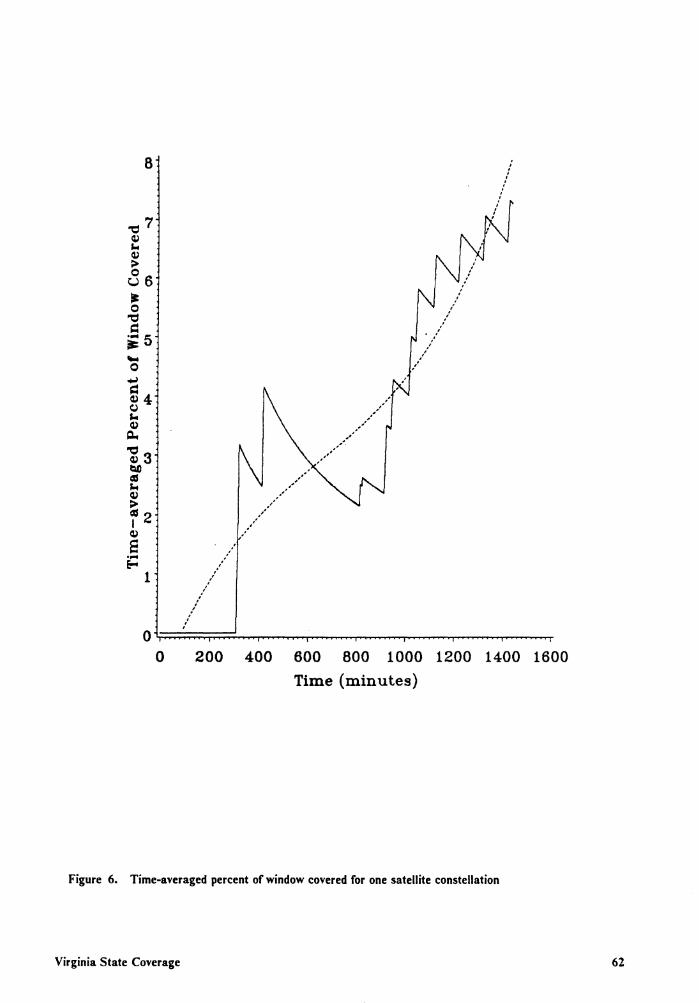
8

'

/ ' '

' '

/ /

,," ' ' '

' ' '

'

' ' ,./

/

Q1.,:;:;:;:;:;:.;:;:;:;:.;:;:;:;:.;:;:....,................,~......,...,.., ...................................... .,...,...,......,...,...,..... ...................... .,..............,............. ........... ~ ..............

0 200 400 600 800 1000 1200 1400 1600 Time (minutes)

Figure 6. Time-averaged percent of window covered for one satellite constellation


30

-0 cu ... cu > 0 u II: 0

-0 20 d .... -= .... 0

+.i d cu CJ ... cu

Q.. -0 cu ~ Cd 10 ... cu > Cd I cu e ....

E-4

..

0 200 400 600 800 1000 1200 1400 1600 Time {minutes)

Figure 7. Time-averaged percent of window covered for three satellite constellation


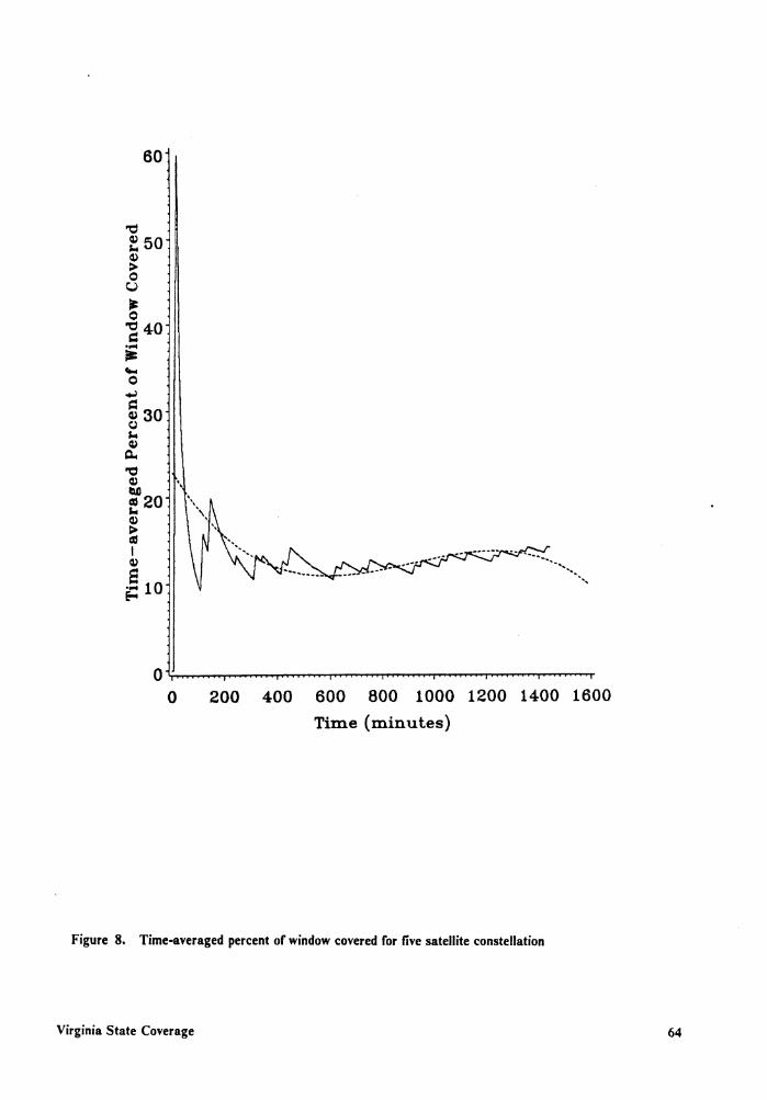
60

'Tj

~ 50 Q,) > 0 u Ir: 0

'Tj 40 c •"'4 ii= .... 0

+J

~ 30 CJ

""' Q) Q.. 'Tj

Q,) . bO as 20 ""' Q,) I> as I Q,) e •"'410 e...

0 200 400 600 800 1000 1200 1400 1600 Time {minutes)

Figure 8. Time-averaged percent of window covered for five satellite constellation


40

ol,:,..,-......... .......-r ........................ ""'T"""........,,..,..,.....r-'""' ......... ......,......,.........,...,......,..................,........,,..,..,........,...,.....'T""""' ............ .,..,...,.,.

0 200 400 600 800 1000 1200 1400 1600 Time (minutes)

Figure 9. Time-averaged percent of window covered for seven satellite constellation


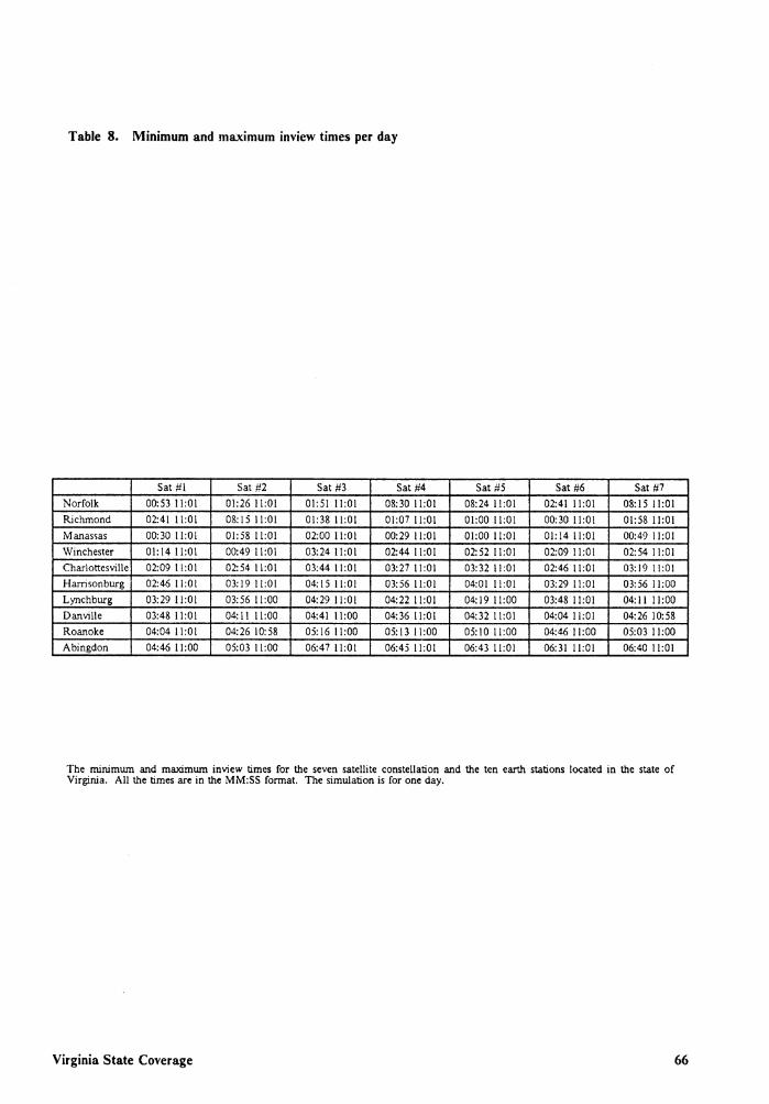
Table 8. Minimum and maximum inview times per day

Sat #l Sat #2 Sat #3 Sat #4 Sat #5 Sat #6 Sat #7 Norfolk 00:53 11:01 01:26 l l:Ol 01:51 11:01 08:30 l l:Ol 08:24 l l:Ol 02:41 l l:Ol 08:15 l l:Ol Richmond 02:41 l l:Ol 08:15 l l:Ol 01:38 l l:Ol 01:07 11:01 01:00 l l:Ol 00:30 ll:Ol 01:58 l l:Ol Manassas 00:30 11:01 01:58 l l:Ol 02:00 l l:Ol 00:29 11:01 01:00 11:01 01:14 11:01 00:49 l l:Ol Winchester 01: 14 11:01 00:49 l l:Ol 03:24 l l:Ol 02:44 l l:Ol 02:52 ll:Ol 02:09 l l:Ol 02:54 l l:Ol Charlottesville 02:09 11:01 02:54 11:01 03:44 11:01 03:27 11:01 03:32 11:01 02:46 11:01 03:19 11:01 Harrisonburg 02:46 11:01 03:19 11:01 04:15 l l:Ol 03:56 11:01 04:01 l l:Ol 03:29 l l:Ol 03:56 11:00 Lynchburg 03:29 l l:Ol 03:56 11:00 04:29 l l:Ol 04:22 11:01 04: 19 11:00 03:48 11:01 04: l l 11:00 Danville 03:48 11:01 04:11 11:00 04:41 11:00 04:36 l l:Ol 04:32 l l:Ol 04:04 l l:Ol 04:26 10:58 Roanoke 04:04 11:01 04:26 10:58 05:16 11:00 05:1311:00 05:10 11:00 04:46 11:00 05:03 11:00 Abingdon 04:46 l 1:00 05:03 11:00 06:47 11:01 06:45 l l:Ol 06:43 11:01 06:31 11:01 06:40 11:01

The minimum and maximum inview times for the seven satellite constellation and the ten earth stations located in the state of Virginia. All the times are in the MM:SS format. The simulation is for one day.


Table 9. Number of inviews and average time of inview per day

Sat #I Sat #2 Sat #3 Sat #4 Sat #5 Sat #6 Sat #7 Norfolk 11 09: 12 11 09:21 11 09:24 IO 10:09 10 10:03 11 09:21 IO 10:02 Richmond II 09:21 10 10:02 14 08:05 14 07:53 14 07:48 13 08:22 13 08:22 Manassas 13 08:22 13 08:22 14 08:06 14 07:52 14 07:49 13 08:24 14 07:48 Winchester 13 08:24 14 07:48 14 08:26 14 08:18 14 08:15 14 08:!4 14 08:15 Charlottesville 14 08:14 14 08:15 14 08:33 14 08:27 14 08:23 14 08:22 14 08:23 Harrisonburg 14 08:22 14 08:23 14 08:41 14 08:36 14 08:32 14 08:31 14 08:32 Lynchburg 14 08:31 14 08:32 14 08:46 14 08:41 14 08:38 14 08:37 14 08:37 Danville 14 08:37 14 08:37 14 08:50 14 08:46 14 08:43 14 08:42 14 08:42 Roanoke 14 08:42 14 08:42 14 08:59 14 08:55 14 08:52 14 08:52 14 08:52 Abingdon 14 08:52 14 08:52 14 09:24 14 09:21 14 09:19 14 09:19 14 09: 19

The number of in views {first column) and the average inview time {second clournn) for the seven satellite constellation and the ten earth stations located in the state of Virginia. The average inview time is in the MM:SS format. The simulation is for one day.


Table 10. Total inview times per day

Sat #I Sat #2 Sat #3 Sat #4 Sat #5 Sat #6 Sat #7 Norfolk 01:41:17 01:43:00 01:43:24 01:41:32 01:40:30 01:42:52 01:40:29 Richmond 01:42:52 01:40:29 01:53: 15 01:50:22 01:49:26 01:48:48 01:48:50 Manassas 01:48:48 01:48:50 01:53:28 01:50: 12 01:49:32 01:49:13 01:49:26 Winchester 01:49: 13 01:49:26 01:58:05 01:56:23 01:55:33 01:55: 17 01:55:30 Charlottesville 01:55:17 01:55:30 01:59:51 01:58:26 01:57:34 01:57:19 01:57:30 Harrisonburg 01:57:19 01:57:30 02:01:38 02:00:27 01:59:37 01:59:26 01: 59: 36 Lynchburg 01:59:26 01:59:36 02:02:48 02:01:44 02:00:56 02:00:46 02:00:50 Danville 02:00:46 02:00:50 02:03:50 02:02:49 02:02:04 02:01:54 02:01:56 Roanoke 02:01: 54 02:01:56 02:05: 54 02:04: 57 02:04:20 02:04: IO 02:04: 14 Abingdon 02:04: IO 02:04: 14 02: 11:39 02: 11:06 02:10:38 02:10:28 02:10:28

The total in view time for the seven satellite constellation and the ten earth stations located in the state of Virginia. The time is in the HH:MM:SS format. The simulation is for one day.


0 100 200 300 400 500 600 700

Window T.ime Bin (Seconds)

Figure 10. Histogram for Virginia using seven satellite constellation


5.3 Summary

The usefulness of Figure 6 on page 62 through Figure 9 on page 65 is that they give a measure of

the coverage for the whole state of Virginia and not just one particular earth station. This is helpful

for the design of a system for remote sensing or vehicle location, where the transmitter could

possibly be anywhere within the state.

With a constellation of one LEO satellite, coverage of the state of Virginia is sporadic and very

minimal. Table 2 on page 21 represents a situation of a single LEO satellite in circular orbit with

two geographically separated earth stations lying directly on the satellite's ground track. The

percentage of time that an earth station in the state of Virginia would be in view of this single

satellite is less than eight percent. This means that, on the average, the earth station will be able

to communicate with this satellite for less than 115 minutes per day.

With a constellation of three LEO satellites, coverage of the state of Virginia becomes a little more

consistent. The percentage of time that an earth station in the state of Virginia would be in view

of this single satellite is approximately nine percent. This means that, on the average, the earth

station will be able to communicate with this satellite for approximately 130 minutes per day.

With a constellation of five LEO satellites, coverage of the state of Virginia becomes a even more


of this single satellite is approximately thirteen percent. This means that, on the average, the earth


With a constellation of seven LEO satellites, coverage of the state of Virginia becomes more


of this single satellite is approximately nineteen percent. This means that, on the average, the earth



6.0 Continental United States Coverage

6.1 Satellite Constellations

The satellite constellations for the analysis of the Continental United States (CO NUS), are identical

to those used for the study of the state of Virginia.

6.2 Statistical Analysis

The nwindowH for the United States is assumed to have the following boundaries:

• North boundary is 48°

• South boundary is 25°

• West boundary is 125°

• East boundary is 70°

Continental United States Coverage 71

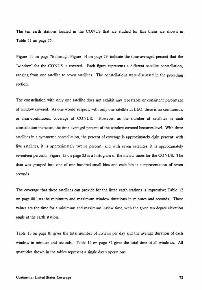
The ten earth stations located m the CONUS that are studied for this thesis are shown m

Table 11 on page 75.

Figure 11 on page 76 through Figure 14 on page 79, indicate the time-averaged percent that the

"window" for the CONUS is covered. Each figure represents a different satellite constellation,

ranging from one satellite to seven satellites. The constellations were discussed in the preceding

section.

The constellation with only one satellite does not exhibit any repeatable or consistent percentage

of window covered. As one would suspect, with only one satellite in LEO, there is no continuous,

or near-continuous, coverage of CONUS. However, as the number of satellites in each

constellation increases, the time-averaged percent of the window covered becomes level. With three

satellites in a symmetric constellation, the percent of coverage is approximately eight percent; with

five satellites, it is approximately twelve percent; and with seven satellites, it is approximately

seventeen percent. Figure 15 on page 83 is a histogram of the inview times for the CONUS. The

data was grouped into one of one hundred small bins and each bin is a representation of seven

seconds.

The coverage that these satellites can provide for the listed earth stations is impressive; Table 12

on page 80 lists the minimum and maximum window durations in minutes and seconds. These

values are the time for a minimum and maximum inview time, with the given ten degree elevation

angle at the earth station.

Table 13 on page 81 gives the total number of inviews per day and the average duration of each

window in minutes and seconds. Table 14 on page 82 gives the total time of all windows. All

quantities shown in the tables represent a single day's operations.


From these three tables it can be concluded that a single LEO satellite with orbits chosen to cover

the United States can provide at least 10 windows of an average duration exceeding 9 minutes per

day for the chosen earth stations.

Performing a statistical analysis on all the inview times for the ten earth stations located in the

CONUS yields the following results.

Number of data points

Mean

Standard deviation

Variance

Skewness

Kurtosis

Covariance

Highest value

Lowest value

10% quantile

25% quantile

50% quantile

75% quantile

90% quantile

Range

75% - 25%

867

576.20 seconds

95.49 seconds

9119.28 seconds

-2.61171 seconds

9.5432 seconds

16.57 seconds

662 seconds

7 seconds

463 seconds

544 seconds

600 seconds

643 seconds

659 seconds

655 seconds

99 seconds

Therefore, fifty percent of inview times have a duration between 544 seconds (9 minutes) and 643

seconds (11 minutes).

The data used for the analysis of the "window" for CO NUS coverage was generated using code

written in Turbo Pascal Version 5.0. The code was run on an IBM PS/2 Model 60 computer.

The computer has a 10 MHz 80286 microprocessor with an 80287 math coprocessor. This code


was written by Stephen H. Goldstein and modified by the author at SAIC. The data used for the

analysis of inview generation was obtained using code written in Fortran 77. The code was run

on an IBM 3090 Model 200 processor complex with 64 megabytes of memory, containing two

processors, with a combined capacity of approximately 28 million instructions per second. These

processors run IBM's VM operating system, VM/XA SPl with CMS Release 5.5.

6.3 Summary

The usefulness of Figure 11 on page 76 through Figure 14 on page 79 is that they give a measure

of the coverage for the whole CO NUS and not just one particular earth station. This is helpful for

the design of a system for remote sensing or vehicle location, where the transmitter could possibly

be located anywhere within the CONUS.

With a constellation of one LEO satellite, CONUS coverage is sporadic and very minimal.

Table 2 on page 21 represents a situation of a single LEO satellite in circular orbit with two

geographically separated earth stations lying directly on the satellite's ground track. The percentage

oftime that an earth station in the CO NUS would be in view of this single satellite is less than seven

percent. This means that, on the average, the earth station will be able to communicate with this

satellite for less than 100 minutes per day.

With a constellation of three LEO satellites, CONUS coverage becomes a little more consistent.

The percentage of time that an earth station in the CO NUS would be in view of this single satellite

is approximately eight percent. This means that, on the average, the earth station will be able to

communicate with this satellite for approximately 115 minutes per day.


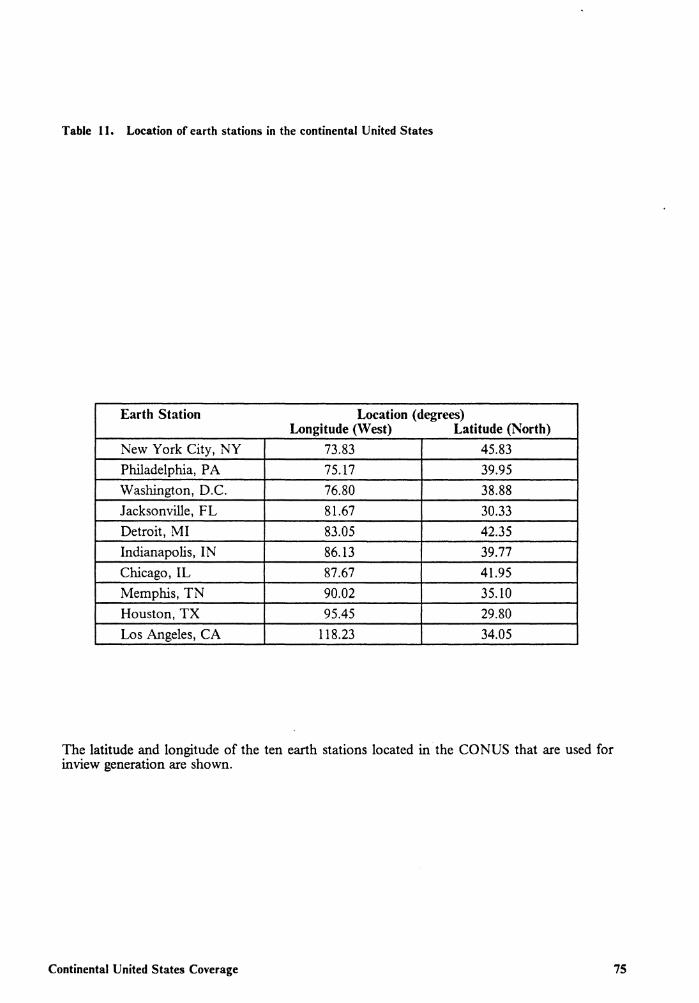
Table 11. Location of earth stations in the continental United States

Earth Station Location (degrees) Longitude (West) Latitude (North)

New York City, NY 73.83 45.83 Philadelphia, PA 75.17 39.95 Washington, D.C. 76.80 38.88 Jacksonville, FL 81.67 30.33 Detroit, MI 83.05 42.35 Indianapolis, IN 86.13 39.77 Chicago, IL 87.67 41.95 Memphis, TN 90.02 35.10 Houston, TX 95.45 29.80 Los Angeles, CA 118.23 34.05

The latitude and longitude of the ten earth stations located in the CO NUS that are used for inview generation are shown.


8

' ' '

/

' '

'

' ' '

' ' ' ' ' '

//

0 200 400 600 800 1000 1200 1400 1600 Time (minutes)

Figure 11. Time-averaged percent of window covered for one satellite constellation


40

~ Q,) ... Q,) :> 830 ~ 0 ~

s:::: .... ;;i:: .... 0 .i

~ 20 Q ... Q,) c... . ~

. . . Q,) . . bAI «I ... Q,) > «I 10 I Q,) e .... ~

o;;....... ............................................ ,....,..... .......... ~~ ........... ......,...~ ............ ..,..... .......... .....,..~ ......... ""r"'~""'"'"'T 0 200 400 600 800 1000 1200 1400 1600

Time (minutes)

Figure 12. Time-averaged percent of window covered for three satellite constellation


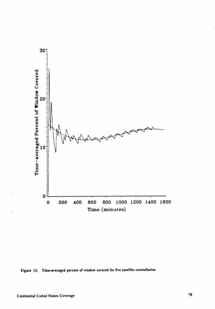
0 200 400 600 800 1000 1200 1400 1600 Time (minutes)

Figure 13. Time-averaged percent of window covered for five satellite constellation


50

0 200 400 600 800 1000 1200 1400 1600 Time (minutes)

Figure 14. Time-averaged percent of window covered for seven satellite constellation


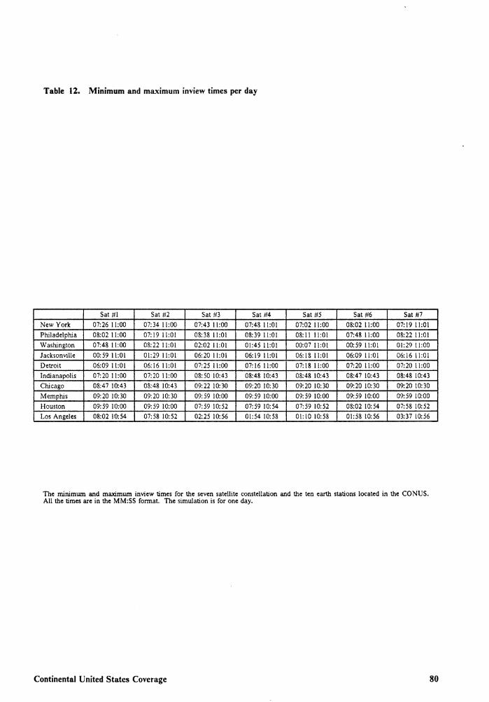
Table 12. Minimum and maximum inview times per day

Sat #l Sat #2 Sat #3 Sat #4 Sat #5 Sat #6 Sat #7 New York 07:26 l l:OO 07: 34 l !:00 07:43 l l:OO 07:48 l l:Ol 07:02 11:00 08:02 l !:00 07:!9 I l:Ol Philadelphia 08:02 l 1:00 07:19 11:01 08:38I1:01 08:39 l l:Ol 08:! l l 1:01 07:48 l 1:00 08:22 I 1:01 Washington 07:48 l 1:00 08:22 I 1:01 02:02 I 1:01 01:45 l l:OI 00:07 I 1:01 00:59 l l:Ol 01:29 I 1:00 Jacksonville 00:59 ll:Ol 01:29 I 1:0! 06:20 l l:Ol 06:19 11:01 06: 18 l l:Ol 06:09 l l:Ol 06:16l1:01 Detroit 06:09 11:01 06:16 11:0! 07:25 11:00 07: 16 11:00 07: 18 l 1:00 07:20 11:00 07:20 11:00 Indianapolis 07:20 11:00 07:20 11:00 08:50 10:43 08:48 10:43 08:48 10:43 08:47 10:43 08:48 10:43 Chicago 08:47 10:43 08:48 10:43 09:22 !0:30 09:20 10:30 09:20 10:30 09:20 10:30 09:20 10:30 Memphis 09:20 10:30 09:20 10:30 09:59 10:00 09: 59 !0:00 09:59 10:00 09:59 10:00 09:59 10:00 Houston 09:59 10:00 09:59 10:00 07:59 10:52 07:59 10:54 07:59 10:52 08:02 10:54 07:58 10:52 Los Angeles 08:02 l 0: 54 07:58 10:52 02:25 10:56 01:54 10:58 01:10 10:58 01:58 10:56 03:37 10:56

The minimum and maximum inview times for the seven satellite constellation and the ten earth stations located in the CONUS. All the times are in the MM:SS format. The simulation is for one day.


Table 13. Number of inviews and average time of inview per day

Sat #1 Sat #2 Sat #3 Sat #4 Sat #5 Sat #6 Sat #7 New York 10 09:47 IO 09:54 IO 09:55 IO 09:55 10 09:46 IO 09:49 10 09:48 Philadelphia IO 09:49 IO 09:48 10 10:04 10 10:04 IO 09:57 10 09:56 10 09:57 Washington 10 09:56 10 09:57 12 08:51 11 09:25 12 08:31 12 08:43 II 09:18 Jacksonville 12 08:43 11 09:18 14 09:20 14 09:18 14 09:16 14 09:15 14 09:15 Detroit 14 09:15 14 09:15 14 09:33 14 09:32 14 09:30 14 09:30 14 09:30 Indianapolis 14 09:30 14 09:30 14 09:52 14 09:51 14 09:50 14 09:50 14 09:50 Chicago 14 09:50 14 09:50 14 09:57 14 09:56 14 09:56 14 09:56 14 09:56 Memphis 14 09:56 14 09:56 14 09:59 14 09:59 14 09:59 14 09:59 14 09:59 Houston 14 09:59 14 09:59 14 09:41 14 09:41 14 09:43 14 09:44 14 09:43 Los Angeles 14 09:44 14 09:43 8 07:55 8 07:28 8 07:30 7 08:22 7 08:25

The number of inviews (first column) and the average inview time (second cloumn) for the seven satellite constellation and the ten earth stations located in the CONUS. The average inview time is in the MM:SS format. The simulation is for one day.


Table 14. Total inview times per day

Sat #I Sat #2 Sat #3 Sat #4 Sat #5 Sat #6 Sat #7 New York 01:37:53 01:39:03 01:39: 12 01:39:14 01:37:42 01:38:13 01:38:00 Philadelphia 01:38:13 01:38:00 01:40:45 01:40:45 01:39:32 01:39:25 01:39:35 Washington 01:39:25 01:39:35 01:46:19 01:43:40 01:42:24 01:44:44 01:42:21 Jacksonville 01:44:44 01:42:21 02: 10:51 02:10:18 02:09:47 02:09:40 02:09:41 Detroit 02:09:40 02:09:41 02:13:53 02:13:33 02: 13:08 02: 13:00 02: 13:00 Indianapolis 02: 13:00 02: 13:00 02: 18: 15 02: 18:03 02: 17:50 02: 17:48 02: 17:45 Chicago 02: 17:48 02:17:45 02: 19:22 02:19:17 02:19:11 02: 19:04 02:19:08 Memphis 02: 19:04 02: 19:08 02: 19:53 02: 19:53 02:19:53 02: 19: 53 02: 19:53 Houston 02:19:53 02: 19:53 02: 15:44 02: 15:45 02: 16:02 02: 16:20 02:16:15 Los Angeles 02: 16:20 02:16:15 01:03:25 00:59: 51 01:00:07 00:58:39 00:59:00

The total inview time for the seven satellite constellation and the ten earth stations located in the CONUS. The time is in the HH:MM:SS format. The simulation is for one day.


130

120

11 0

100

.a 90 i:Q 80 1 r..:i 70 .a "" 60 CD .a

~ 50

40

30

20

10

0

0 100 200 300 400 500 600 700

Window Time Bin (Seconds)

Figure 15. Histogram for CONUS using seven satellite constellation


With a constellation of five LEO satellites, CONUS coverage becomes a even more consistent.

The percentage of time that an earth station in the CO NUS would be in view of this single satellite

is approximately twelve percent. This means that, on the average, the earth station will be able to

communicate with this satellite for approximately 173 minutes per day.

With a constellation of seven LEO satellites, CONUS coverage becomes more consistent. The

percentage of time that an earth station in the CO NUS would be in view of this single satellite is

approximately seventeen percent. This means that, on the average, the earth station will be able

to communicate with this satellite for approximately 245 minutes per day.


7.0 Simulation Study of Low-Earth-Orbit Satellite

Systems

7.1 Compressed Text

After examination of a typical document, the average number of characters per A4 page of text is

2,700. An A4 page is simply a standard (8 1/2 by 11 inch) document page. Working backwards

from 2, 700 characters, that amount is comparable to a doubled spaced page with 80 characters on

every line, or a single spaced page with an average of 40 characters per line. American National

Standard Code for Information Interchange (ASCII) text files are notoriously inefficient. ASCII

takes advantage of only seven data bits in an eight bit byte, and furthermore, plain text contains

many repeated sequences of characters. There are widely implemented compression algorithms

which yield dramatic compression of text files. The program ARC.EXE for the IBM PC family

of computers was tested and this regularly compresses ASCII text files to 60 percent of their original

size. Since memory is one of the limited resources on satellite payloads, earth stations should only

send compressed text to one another. Thus, the subjective page of text can now be stored in 2,700

x 0.6 = 1,700 bytes [22].

Simulation Study of Low-Earth-Orbit Satellite Systems 85

7.2 Satellite Path Geometry

To determine the minimum altitude for satellites to be visible to one another, it is necessary to first

look at the geometry of the problem. In this study, the satellites will be in a constellation that is

symmetric. The constellation will place the satellites equally spaced about the equator at the start

of the simulation. From the beginning of the simulation until the end, which is one day in

simulation time, the satellites will remain in their symmetric constellation. This is a result of the

other initial orbital elements entered as parameters in the simulation. The satellites all have zero

eccentricity. As one would suspect, any constellation with fewer than three satellites cannot have

mutual visibility. Also, as will be shown later for any constellation with greater than thirteen or

fourteen satellites, the altitude for mutual visibility is not the prime concern. With those

constellations, the minimum altitude is below 200 kilometers and will therefore be greatly affected

by atmospheric conditions.

Equations pertinent to the study of this problem are:

RE h=------RE cos(-18_~-o )

( 180° ) d= 2(RE+ h) sin ~

(10)

( 11)

(12)

where RE is the radius of the earth, which is approximately 6,370 kilometers, d is the distance

between the two satellites, N is the number of satellites in the constellation, and h is the altitude

of the satellites. Table 15 on page 89 shows that for satellite constellations with greater than

thirteen satellites, the required altitude for communication links does not depend upon the

minimum altitude of the satellites, but rather the requirement that they remain above the earth's


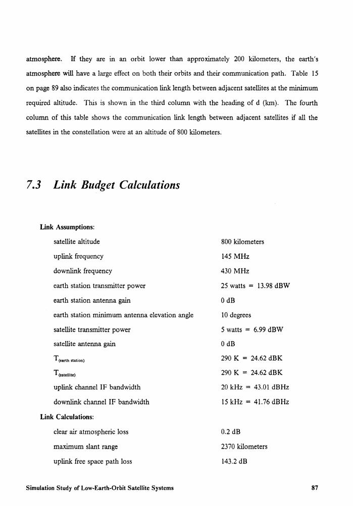
atmosphere. If they are in an orbit lower than approximately 200 kilometers, the earth's

atmosphere will have a large effect on both their orbits and their communication path. Table 15

on page 89 also indicates the communication link length between adjacent satellites at the minimum

required altitude. This is shown in the third column with the heading of d (km). The fourth

column of this table shows the communication link length between adjacent satellites if all the

satellites in the constellation were at an altitude of 800 kilometers.

7.3 Link Budget Calculations

Link Assumptions:

satellite altitude

uplink frequency

downlink frequency

earth station transmitter power

earth station antenna gain

earth station minimum antenna elevation angle

satellite transmitter power

satellite antenna gain

T (earth station)

T(satelllte)

uplink channel IF bandwidth

downlink channel IF bandwidth

Link Calculations:

clear air atmospheric loss

maximum slant range

uplink free space path loss

Simulation Study of Low-Earth-Orbit Satellite Systems

800 kilometers

145 MHz

430 MHz

25 watts = 13.98 dBW

0 dB

10 degrees

5 watts = 6.99 dBW

0 dB

290 K = 24.62 dBK

290 K = 24.62 dBK

20 kHz = 43.01 dBHz

15 kHz = 41.76 dBHz

0.2 dB

2370 kilometers

143.2 dB

87

Figure 16. Satellite path geometry model


Table 15. Minimum altitude for link between satellites

N (no. of satellites) h (km) d (km) distance (km) 3 6370.00 22066.33 4 2638.54 12740.00 5 1503.75 9256.15 6 985.44 6355.44 7 700.17 6135.26 6221.89 8 524.84 5277.08 5487.68 9 408.81 4636.98 4904.57

10 327.81 4139.48 4431.30 11 268.92 3740.80 4040.04 12 224.71 3413.67 3711.46 13 190.64 3140.13 3431.79 14 163.82 2907.82 3190.95 15 142.31 2707.82 2981.45

The first column indicates the number of satellites in a constellation spaced equally about the earth in one orbital plane. The second column indicates the required altitude (or height) for the satellites to have a direct communication path. The third column indicates the distance between two adjacent satellites in the mentioned constellation. The last column indicates the distance between two adjacent satellites at an altitude of 800 kilometers.


downlink free space path loss

EIRP(earth station)

EIRP(satellite)

Boltzman' s constant

152.6 dB

13.98 dBW

6.99 dBW

-228.6 dBW/K/Hz

The following equations are used to determine the maximum slant range for a satellite in a circular,

800 kilometer orbit [23].

. RE cos E sma= RE+ h (13)

e = 90° -E-a (14)

r= (RE+ h) cos 8 - RE

sin£ (15)

where a is the nadir angle, E is the minimum elevation angle of the earth station, RE is the radius

of the earth, h is the satellite altitude, e is the central angle, and r is the slant range. The following

values will be used in the above equations:

RE= 6370 kilometers

E= 10°

h = 800 kilometers

Therefore:

a= 61.04°

e = 18.96°

r = 2365.97 kilometers


Therefore, the maximum distance from an earth station to a satellite in an 800 kilometer orbit is

approximately 2,370 kilometers. The free space path loss can then be calculated from the following

equation [ 18).

(16)

where R is the distance from the satellite's antenna to the earth station's antenna and A is the

wavelength of the frequency being transmitted. This gives a free space path loss of 143.2 dB on the

uplink (145 MHz) and 152.6 dB on the downlink (430 MHz). Free space path loss is a not a loss

in the sense of power being absorbed; it accounts for the way energy spreads out as an

electromagnetic wave propagates away from a transmitting source.

Using the above assumptions and calculations, a simple link budget can be computed for an 800

kilometer altitude satellite in circular orbit, with a minimum earth station elevation angle of ten

degrees.

The carrier-to-noise ratio is then given by the following equation [ 18).

( ~ ) up = EIRP<•arth station> - free space path loss(uplink> +

G(satellite) - T(satellite) - k - B(satellite) dB

, c) ( N' up= 13.98 - 143.2- 0.2 + o- 24.62 + 228.6- 43.01

( ~ )up= 31.55 dB

( NC ) = EIRP<satenit•> - free space path loss(downtink> + l down

G(earth station) - T(earth station) - k - B(earth station) dB


( NC ) = 6.99- 152.6- 0.2 + 0 - 24.62 + 228.6- 41.76 l down

( NC ) = 16.40 dB down

There is also a margin of 6 dB, which consists of 2 dB for receiver losses, 3 dB for polarization

losses, and 1 dB for transmitter losses, which has not been included yet [22J. With the inclusion

of the 6 dB margin, the C/N on the up and down links are:

( ~ lP = 25.55 dB and ( N~ ) = 10.40 dB l down

The ratio Eb/N0 , the bit energy, Eb, to noise spectral density, N0 , is a quantity for system calculations

and performance comparisons. However, in practical measurements it is more convenient to

measure the average carrier-to-average noise (C/N) power ratio. The bandwidth is the 3 dB

bandwidth of the receiver. THe follwoing analysis also assumes that BN = Bw. The system is that

of a non-optimum design (not a matched filter design), therefore BwTb = 1.56. The optimum

bandwidth for FSK depends on the deviation. The 15 kHz bandwidth is used to allow for some

shift in the actual frequency of the signal in the IF due to the changing Doppler shift. The following

simple relations are useful for the Eb/N0 to (C/N) transformations [7]

(17)

(18)

(19)

(20)


The Eb/N0 ratio equals the product of the (C/N) ratio and of the receiver noise bandwidth-to-bit

rate ratio (B,./Rb)· The following values will be used in the above equations:

Rb= 9600 bps

Bw = 15 kHz

The following equation is obtained from equation (19)

(21)

or, expressed in decibels,

(22)

The coherent frequency-shift keying (FSK) modulation/demodulation method has a probability of

error, P., given by [71

(23)

Therefore, using equation (21), the required (C/N) can be found. On the "good" link, with a BER

of 2.5 x 10-s,

and, therefore, using equation (21),

c N=9.85dB

On the "bad" link, with a BER of 4.0 x 10-4 ,


and, therefore, using equation (21),

c N= 8.04 dB

7.4 Doppler Shift Frequency

7 .4.1 Introduction

In general, a Doppler effect is experienced whenever there is relative motion between a source and

an observer. When the source and the observer are moving toward each other, the frequency

perceived by the observer is higher than the frequency of the source. When the source and the

observer are moving away from each other, the frequency perceived by the observer is lower than

the frequency of the source. The Doppler effect (named after Christian Johann Doppler,

1803-1853) is this apparent shift in frequency when either the source of oscillation or an observer

of the oscillation is in motion. He first observed this shift in 1842. Two primary questions related

to Doppler shift are of interest to satellite users:

1. What will the actual Doppler shift be on a given link at a given time?

2. What is the maximum Doppler shift that can be expected on a given link?

A monitor that is at rest with respect to a transmitter will measure a frequency J., while an observer

who is moving with respect to the transmitter will measure a different frequency, f '. The

relationship is given by [ 5]


I v, I =lo±c:lo (24)

where f0 is the frequency as measured by a monitor at rest with respect to the source (source

frequency), f' is the frequency as measured by an observer who is moving with respect to the source

(apparent frequency), v, is the relative velocity of the observer with respect to the source, and c is

the speed of light. The sign convention used is that when the distance between the source and the

observer is decreasing, a "+ " sign is used (f ' > f0 ) and when the distance between the source and

the observer is increasing, a "." sign is used (f' < f0 ) • Equation (24) is often written as

v, 6.f =I I - lo = ± c lo (25)

In the LEO case, there is a maximum and minimum Doppler shift that can be seen by any earth

station. During most orbits, however, most stations will observe a shift somewhere between these

two extremes. For a circular orbit the two limits remain constant. The two factors that contribute

to the relative velocity term in equation (24) are:

I. Rotation of the earth about the North-South axis

2. Satellite motion in the orbital plane

In any given situation these two factors can be combined (velocities add as vectors) to produce a

relative velocity having a magnitude that can range from the arithmetic difference to the arithmetic

sum of the two components. Since the objective is to determine worst-case limits for a practical

situation, it is only necessary to calculate each contribution separately and then form the sum and

difference.


--- - - - - ~te/fit - ........ e Patt, .....

.....

earth center

Figure 17. Geometry for computing contribution to worst case Doppler shift from satellite motion only (circular orbit)


7 .4.2 Rotation of the Earth

The earth rotates about its North-South axis at an angular velocity of

wE = 360 de:ees = 15 degrees = 0_25 de_grees = 4_167 x 10_3 degrees = 7_272 x 10_s radians ay hour rmnute second second

The tangential velocity of a point on the surface of the earth at latitude q,, is [SJ

(26)

where RE is the radius of the earth, <P is the latitude, and wE is the angular velocity of the earth (in

radians). The maximum value of vE will occur at the equator, vE< max>= 463.239 meters/second.

To obtain an idea of the Doppler shift that arises exclusively from the rotation of the earth, assume

a link frequency of 430 MHz and an earth station on the equator that sees a satellite due east on

the horizon. In this position, the tangential velocity of the earth and the relative earth

station-to-satellite velocity are equal. Using equation (25),

~J; - 463·239 x (430 x 106) = 663.98 Hz max(earth) - 3 X l08 (27)

However, at an earth station located in Blacksburg, Virginia, which has a latitude of 37.229 degrees,

the associated Doppler due to earth rotation is (vE = 368.842),

~r 368·84? x (430 x 106) = 528.67 Hz '.!(earth)= 3 x 10

(28)

Observed Doppler shifts are usually much larger. Therefore, the contribution of the satellite orbital

motion to Doppler shift must be very important.


7.4.3 Satellite Motion

The earth station that sees the largest relative velocity lies in the orbital plane and sees the spacecraft

at zero degree elevation angle. The velocity (in meters per second) of a satellite in a circular orbit

is given by [SJ

v2=_G_IM __ = 3.986x 1014

(RE+ h) (RE+ h) (29)

where G is the gravitational constant (G = 6.67 x 10-11 m3/ kg sec2), M is the mass of the earth

(M = S.98 x 1024 kg) , and h is the satellite's altitude. The maximum relative velocity (in meters

per second) seen by the earth station is [SJ

RE v, = v cos f3 = v (RE+ h) (30)

where Re. is the radius of the earth, vis the magnitude of the satellite's velocity, and vr is the relative

velocity of the observer with respect to the source. The Doppler shift frequency (in hertz), given

a specific transmitter frequency, is [SJ

(31)

The following values will be used in the above equations:

RE= 6370 kilometers

h = 800 kilometers

fo=430 MHz

Therefore:

v = 74S6.0S meters per second


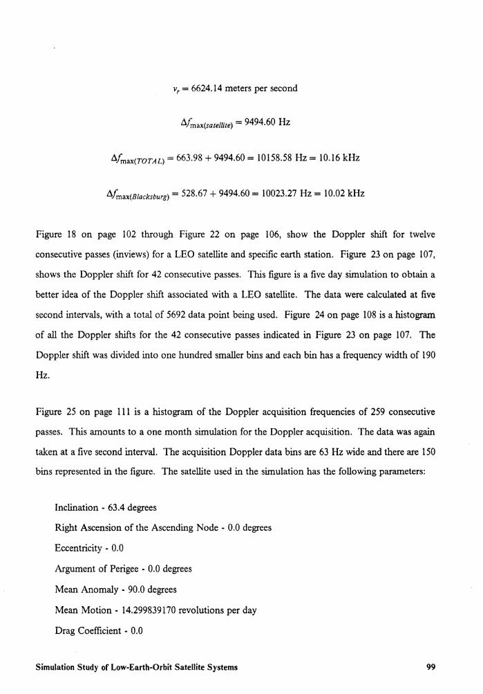
v, = 6624.14 meters per second

fi.fmax(satellite) = 9494.60 Hz

fi.fmax(TOTAL) = 663.98 + 9494.60 = 10158.58 Hz= 10.16 kHz

fi.fmax(Blacksburg) = 528.67 + 9494.60 = 10023.27 Hz= 10.02 kHz

Figure 18 on page 102 through Figure 22 on page 106, show the Doppler shift for twelve

consecutive passes (inviews) for a LEO satellite and specific earth station. Figure 23 on page 107,

shows the Doppler shift for 42 consecutive passes. This figure is a five day simulation to obtain a

better idea of the Doppler shift associated with a LEO satellite. The data were calculated at five

second intervals, with a total of 5692 data point being used. Figure 24 on page 108 is a histogram

of all the Doppler shifts for the 42 consecutive passes indicated in Figure 23 on page 107. The

Doppler shift was divided into one hundred smaller bins and each bin has a frequency width of 190

Hz.

Figure 25 on page 111 is a histogram of the Doppler acquisition frequencies of 259 consecutive

passes. This amounts to a one month simulation for the Doppler acquisition. The data was again

taken at a five second interval. The acquisition Doppler data bins are 63 Hz wide and there are 150

bins represented in the figure. The satellite used in the simulation has the following parameters:

Inclination - 63.4 degrees

Right Ascension of the Ascending Node - 0.0 degrees

Eccentricity - 0.0

Argument of Perigee - 0.0 degrees

Mean Anomaly - 90.0 degrees

Mean Motion - 14.299839170 revolutions per day

Drag Coefficient - 0.0


Frequency - 430.0 MHz

The earth station used in the simulation has the following parameters:

Location - Blacksburg, Virginia

Latitude - 37.229 degrees North

Longitude - 80.438 degrees West

Height - 646 meters above sea level

Timezone - EDT4

A list of the Doppler frequencies required to acquire the signal is shown in Table 16 on page 109.

The minimum elevation angle of the earth station was also varied from zero to twenty degrees.

The corresponding Doppler frequencies are shown. The ten degree minimum elevation angle is the

column of interest to this study. Values of Doppler acquisition frequencies ranging from 3716 to

9052 Hz are shown in this column. Table 18 on page 113 contains a few different items that are

relevant to the study of Doppler shift. The second column of this table, labeled Doppler Range,

indicates the beginning and ending Doppler frequency for each individual pass. The third column,

labeled Total Time, is the number of seconds corresponding to the Doppler Range. Columns four

through nine are the time, in seconds, of a "restricted" pass. The restriction on the pass is the

Doppler Cut-off Frequency. If the receiver had to cut-off the incoming signal at the indicated

frequency limit, the pass time would be reduced to the number of seconds indicated in the column.

Perfonning a statistical analysis on all the Doppler shifts for 42 consecutive passes for an earth

station located at Blacksburg, Virginia yields the following results.

Number of data points

Mean

Standard deviation

Variance

Skewness


5692

-63.46 Hertz

5791.28 Hertz

33538868 Hertz

0.016793 Hertz

100

Kurtosis -1.2747 Hertz

Covariance -9125.32 Hertz

Highest value 9220 Hertz

Lowest value -9213 Hertz

10% quantile -8121 Hertz



75% quantile 5136 Hertz

90% quantile 8074 Hertz

Range 18433 Hertz

75% - 25% 10381 Hertz

The next table, Table 19 on page 114, presents the mean time in the restricted window, as well as

the standard deviation and variance. Both Table 18 and Table 19 assume a minimum elevation

angle of the earth station to be zero degrees. Since the actual minimum elevation angle must be

greater than zero degrees, the duration of each pass represented in these tables will be reduced. One

can compare these tables to Table 16 on page 109 to obtain an idea of the reduction in pass time.

An illustration of the rate of change of the Doppler shift is shown in Figure 26 on page 112. This

is necessary to obtain an idea if the transceivers available can accommodate this change in the

received frequency. The maximum rate of change of the Doppler frequency is approximately 82

Hz per second. This value is sufficiently low that the transceivers can easily accommodate this rate

of change.

Simulation Study of Low-Earth-Orbit Satellite Systems IOI

10000

8000

6000

4000 --2 m 2000 = -~ :a 0 I'll ... m -f:lo f:lo 0 -2000 ~

-4000

-6000

-8000

-------- Pass No. I •••••••••••••••••••••••••••· P3SS No. Z ------------------· Pass No. 3 ------------ P3SS No. 4 ------· P:iss No. 5 ------ P3SS No. 6

P3SS No. 7 --·-·-·-·-·-·-·-Pass No. 8 -·-·-----·-P3SS No. 9 -------·-Pass No. 10 ----- --- P:iss No. 11 ·-------Pass No. 12

0 100 200 300 400 500 600 700 800 900 1000

Time (seconds)

Figure 18. Doppler shift for zero degree elevation angle and above


10000

8000

6000

4000 --2 II 2000 = -~ :a 0 !'I.I ... II -s:a. s:a. 0 -2000 i:::I

-4000

-6000

-8000

-10000

0 100 200 300

·•••••••••••••••••••••••••••· Pass No. 2 ·------------------· Pass No. 3 ·------Pass No. S ------Pass No. 6 -------- Pass 1'o. 7 -·-·--·-Pass No. 10 ----- --- Pass No. 11 ------- Pass No. 12

400 500 600 700

Time (seconds)

Figure 19. Doppler shift for five degree elevation angle and above


800

103

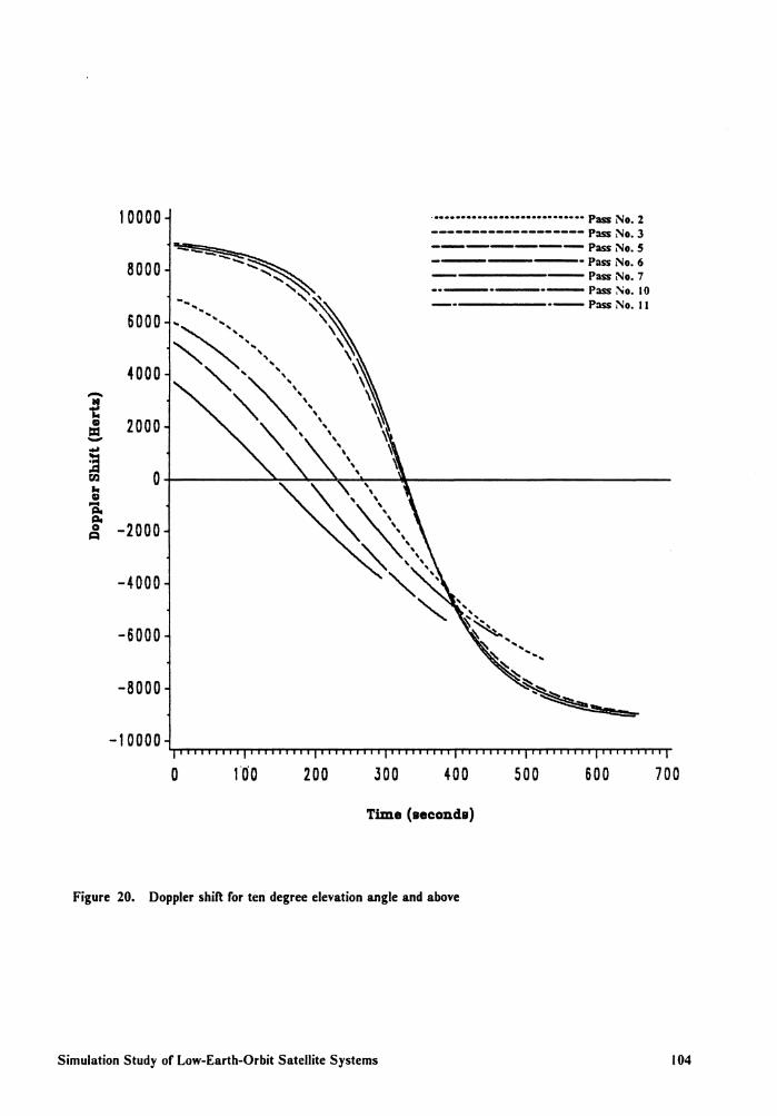
10000

8000

6000

4000 --2 D 2000 = -~

:a 0 I'll .. D -~ ~ 0 -2000 ~

-4000

-6000

-8000

-10000

0 1'00 200 300

·•••••••••••••••••••••••••••• Pass No. 2 -------------------Pass No. 3 -------Pass No. S ----·Pass No. 6 ------ Pass No. 7 ··-·-·-Pass No. 10 -----·-Pass No. 11

400 500 600

Time (seconds)

Figure 20. Doppler shift for ten degree elevation angle and above


700

104

-N·

t = -~ :a rn

9000

7000

5000

3000

1000

! -1000 ,:a. i:a. 0

Q -3000

-5000

-7000

-9000

••••••••••••••• •••••••••••· Pass No. 2 ------------------Pass No. 3 ------·Pass No. S -----·Pass No. 6 -·-·----Pass No. 10

-----·-Pass No. ll

.........................................................................................................................................................................................

0 100 200 300 400 500 600

Time (seconds)

Figure 21. Doppler shift for fifteen degree elevation angle and above


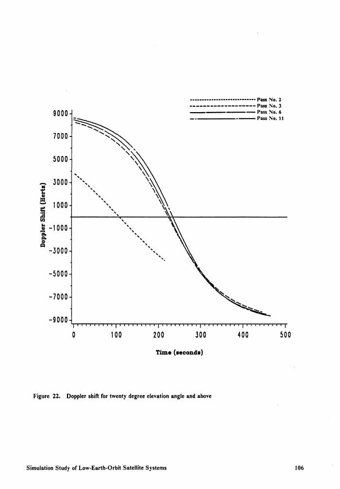
9000

7000

5000

- 3000 N t GI = - 1000 ~ :a

r:ll ... -1000 GI -,:a, ,:a, 0 ~

-3000

-5000

-7000

-9000

~ ..................

~'

····-······················· Pass No. 2 -------------------Pass No. 3 ------Pass No. 6 -----·--Pass No. 11

,, " ... , ,, " ' ' ... " ' ' ' ' ' ' '\ ' ' ' ~ ...

' ' ' ' ' ' ... ' ' ' ' ... ' ... ... ... .

...................................................................................................................................................................................................

0 100 200 300 400 500

Time (seconds)

Figure 22. Doppler shift for twenty degree elevation angle and above


~ --65 t.. cu ...... c. c. 0 c

10000

8000

6000

4000

2000

-2000

-4000

-6000

-8000

-10000

0 100 200 300 400 500 600 700 800 900 1000 Time (seconds)

Figure 23. Plot of all Doppler frequencies for forty-two consecutive passes


300

200 .a l=Q .cl Q as

r-1 .a "" CD

j 100

0 i..,......,_,.........., ....... -.-....... -.-~-.-..-.-.-......... ~ ......... ~ ......... ~ ........ --...-.-.-...-.-.-............... -.-..............

-10000 -5000 0 5000 10000

Doppler Shift Bin (Hertz)

Figure 24. Histogram for all Doppler using a one satellite constellation


Table 16. Doppler acquisition frequencies in hertz for a 430 MHz carrier frequency

Minimum Elevation Angle (degrees) Pass No. 0 5 to 15 20

1 4489 ---- ---- ---- ----2 8071 7653 6956 5769 3838 3 9120 9050 8878 8620 8268 4 4641 .......... ---- . ......... ... ........

5 7518 6764 5229 2396 ............

6 9159 9102 8971 8756 8456 7 6945 5829 3716 ---- ----8 3105 ---- ---- ---- ----9 3940 ---- ............ ---- ----to 7669 6997 6000 4276 ...........

11 9200 9167 9052 8885 8630 12 6118 4280 ---- ........... ----

The Doppler acquisition frequency for the twelve consecutive passes of a satellite in LEO at an altitude of 800 kilometers. The minimum earth station antenna elevation angle is varied from zero to twenty degrees. The earth station is located at Blacksburg, Virginia.


Table 17. Doppler acquisition frequencies statistics

Minimum Elevation Angle (degrees) 0 5 10 15 20

No. of Data Pts 259 194 153 125 102 Mean 6605.13 6859.27 6966.90 6858.34 6760.11

Stnd. Deviation 2275.52 2237.97 2074.03 2116.25 2041.57 Variance 5177987 5008504 4301583 4478503 4167995 Skewness -0.543513 -0.901072 -0.912141 -1.08749 -1.13712 Kurtosis -1.03657 -0.201833 -0.172087 0.412543 0.361528

Covariance 34.4508 32.6269 29.7697 30.8565 30.2002 Highest Value 9223 9191 9085 8917 8675 Lowest Value 2003 837 1105 161 795 10% Quantile 3182 3201 3814 3565 3428 25% Quantile 4685 5344 5636 5465 5352 50% Quantile 7190 7465 7507 7578 7587 75% Quantile 8718 8820 8784 8643 8426 90% Quantile 9159 9131 9029 8869 8645

Range 7220 8354 7980 8756 7880 75% - 25% 4033 3476 3148 3178 3074

Statistics generated from the forty-two consecutive passes of a satellite in LEO at an altitude of 800 kilometers. The earth station is located at Blacksburg, Virginia. The data in this table is in the units of Hertz.


0 1000 2000 3000 4000 5000 6000 7000 8000 9000 10000

Doppler Shift Bin (Hertz)

Figure 25. Histogram for Doppler acquistion frequencies for five varying elevation angles


90

80

1 0

0

0 100 200 300 400 500

--------Pass No. I ····························Pass No. 2 ------------------· Pass No. 3 ------------ Pass No. 4 ------·Pass No. 5 ------Pass No. 6 ---------Pass No. 7 ·--------------- Pass No. 8 -----------Pass No, 9 -------Pass No. 10 --- -----Pass No. 11 ---------Pass No. 12

600 700 800 900 1000

Time (seconds)

Figure 26. Rate of change of Doppler shift


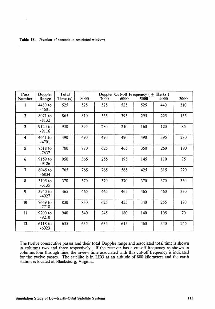
Table 18. Number of seconds in restricted windows

Pass Doppler Total Doppler Cut-off Frequency ( ± Hertz ) Number Range Time (s) 8000 7000 6000 5000 4000 3000

I 4489 to 525 525 525 525 525 440 310 -4601

2 8071 to 865 810 535 395 295 225 155 -8132

3 9120 to 930 395 280 210 160 120 85 -9116

4 4641 to 490 490 490 490 490 395 280 -4701

5 7518 to 780 780 625 465 350 260 190 -7637

6 9159 to 950 365 255 195 145 110 75 -9126

7 6945 to 765 765 765 565 425 315 220 -6834

8 3105 to 370 370 370 370 370 370 350 -3135

9 3940 to 465 465 465 465 465 460 330 -4027

10 7669 to 830 830 625 455 340 255 180 -7718

11 9200 to 940 340 245 180 140 105 70 -9210

12 6118 to 635 635 635 615 460 340 245 -6023

The twelve consecutive passes and their total Doppler range and associated total time is shown in columns two and three respectively. If the receiver has a cut-off frequency as shown in columns four through nine, the inview time associated with this cut-off frequency is indicated for the twelve passes. The satellite is in LEO at an altitude of 800 kilometers and the earth station is located at Blacksburg, Virginia.


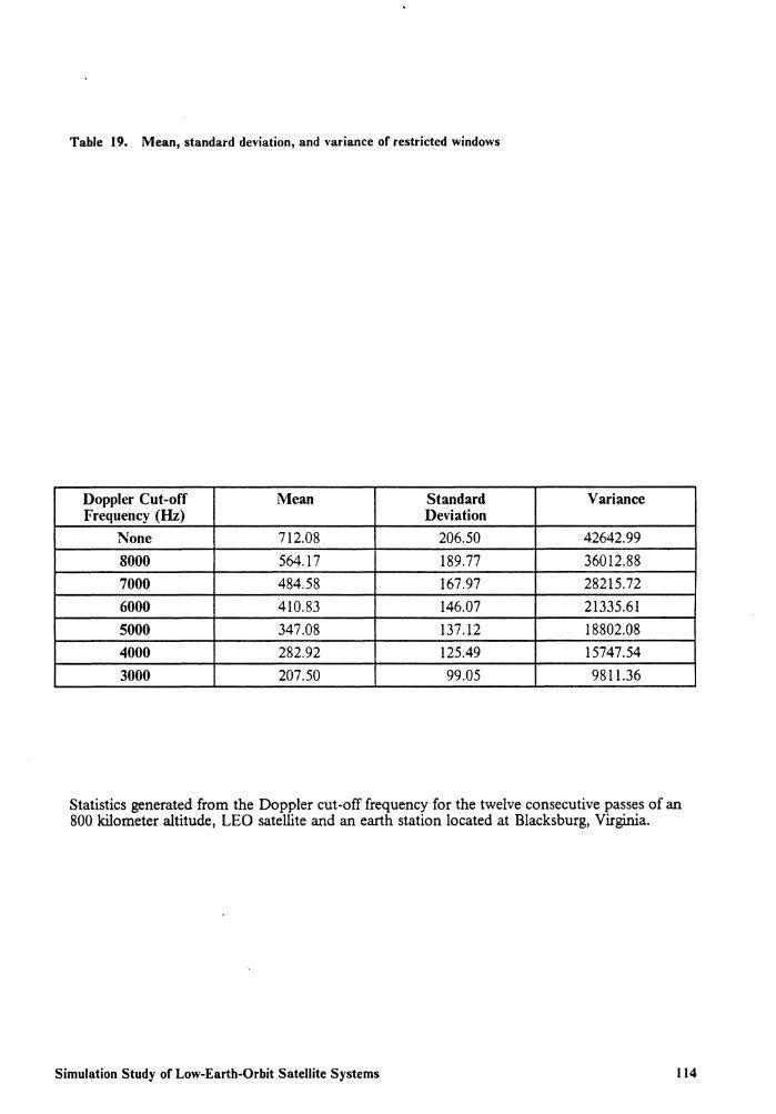
Table 19. Mean, standard deviation, and variance of restricted windows

Doppler Cut-off Mean Standard Variance Frequency (Hz) Deviation

None 712.08 206.50 42642.99 8000 564.17 189.77 36012.88 7000 484.58 167.97 28215.72 6000 410.83 146.07 21335.61 5000 347.08 137.12 18802.08 4000 282.92 125.49 15747.54 3000 207.50 99.05 9811.36

Statistics generated from the Doppler cut-off frequency for the twelve consecutive passes of an 800 kilometer altitude, LEO satellite and an earth station located at Blacksburg, Virginia.


8.0 P ACSAT Scenario

8.1 Introduction

PA CSA T is a proposed system much like a bulletin board except that it will be onboard a future

AMSAT spacecraft. Having as much as two megabytes of memory, PACSAT will fly in LEO.

PA CSA T will enable a low-power earth station with relatively unsophisticated antenna systems to

leave and retrieve messages with PACSAT. The PACSAT payload will provide a communications

link between scientific, humanitarian and development workers and projects in remote areas of the

world and Volunteers in Technical Assistance (VITA) headquarters in the United States.

The University of Surrey, UK, is constructing UoSAT D, a small spacecraft which carries the

PACSAT Communications Experiment (PCE). PCE provides store-and-forward capabilities to

suitably equipped earth stations. The launch of the UoSA T D payload with the PCE capability

is scheduled for July 1989 by Ariane rocket. The Ariane launch will result in a polar orbit at an

altitude of about 800 kilometers. PCE is in two parts. An amateur radio section will provide

store-and-forward to amateur radio operators using the 2m/70cm up/down bands. A separate

P ACS AT Scenario 115

transmitter-receiver package will provide non-amateur frequencies for users, subject to FCC/IRAC

agreement. The proposed frequencies are 149 MHz up and 430 MHz down.

The PCE experiment is based on a 9600 bps data rate for up and down links. Various forms of

FSK are being considered by UoSAT for the downlink. AFSK appears to be the certain choice for

the uplink. Since 9600 bps is definite, the only variables are deviation and bandwidth. Most FSK

systems use a deviation close to the bit rate, and the optimum receiving bandwidth is about 1.1

Rb [22].

8.2 Types of Earth Stations

VITA predicts four types of earth stations used for the PCE. The first is a portable model that can

be contained in a small brief case. For this reason, a laptop, ruggedized personal computer is

needed. Also required is a TNC, dual-band VHF /UHF transceiver, modem, batteries, and a small

antenna. Twenty-five earth stations of this type are expected. Each of which would have a daily

uplink of 2 A4 pages of text, and a daily downlink of the same.

The second is a small fixed model. The primary difference between this model and the portable

model is that this one will use a semi-permanent antenna and perhaps a desktop personal computer.

Most of these stations will use a permanent but non-steered antenna, or even a manually steered

antenna. Twenty-five earth stations of this type are expected. Each of which would have a daily

uplink of 5 A4 pages of text, and a daily downlink of the same.

The third is a base station, which is a permanent earth station installed in locations where there is

mains power available and a structure for mounting steered, auto-tracking antennas. Twelve earth


stations of this type are expected. Each of which would have a daily uplink of 25 A4 pages of text,

and a daily downlink of the same.

The fourth and final type of earth station is the VITA Command Station. This will be located at

VITA headquarters and will be the PA CSA T Command Station. The Command Station will have

to maintain and manage the PA CSA T messaging system. The earth station will be a fixed station

with automatic tracking antennas and a full-featured general purpose computer. The Command

Station should also have a large hard disk for data storage and a non-volatile storage system, such

as magnetic tape or CD ROM. One earth station ofthis type is expected. This station would have

a daily uplink of 350 A4 pages of text, and a daily downlink of the same.

Organizations other than VITA have shown interest in using the PA CSA T facilities. For the

purpose of this thesis, the non-VITA earth stations will fall into one of the four aforementioned

categories of earth stations. As many as 500 of these non-VITA earth stations are anticipated.

There will be 200 small fixed earth stations, that will have a daily uplink of 5 A4 pages of text.

There will also be 300 portable earth stations, each of which will have a daily uplink of 2 A4 pages

of text.

8.3 System Analysis

The scenario set up below is based on PACSAT. The analysis will assume a link bit rate of 9600

bps and a satellite memory capacity of 4 megabytes. First, the amount of data that might be

uplinked to the satellite must be determined. If all of the proposed earth stations were to upload

all their information to the satellite, and the satellite were to hold it all, the amount of information

uploaded would be 2,350 A4 pages of text. This figure is obtained as follows:

VITA Portable Stations 25 x 2 = 50


VITA Small Fixed Stations 25 x 5 = 50

VITA Base Stations 12 x 25 = 300

VITA Command Station x 350 = 350

non-VITA Portable Stations 300 x 2 600

non-VITA Small Fixed Stations 200 x 5 = 1,000

TOTAL = 2,350

Using the ideas developed in Chapter 3, the time required to transmit the expected number of A4

pages can now be determined. The Portable Stations will transmit 2 pages with 1,700 compressed

bytes of information per page. This yields 3,400 bytes of data to be transmitted. The Small Fixed

Stations will transmit 5 pages with 1, 700 compressed bytes of information per page. This yields

8,500 bytes of data to be transmitted. The Base Stations will transmit 25 pages with 1,700

compressed bytes of information per page. This yields 42,500 bytes of data to be transmitted. The

Command Station will transmit 350 pages with 1,700 compressed bytes of information per page.

This yields 595,000 bytes of data to be transmitted.

First, consider how much time is required to transmit the above listed figures for the individual

earth stations. On the "good" link, as described in Section 3.6, it will require the following time to

transfer the information for each station.

BYTES OF DATA

3,400

8,500

42,500

595,000

NUMBER OF SECONDS

3.26

8.14

40.71

569.92

NUMBER OF MINUTES

0.054

0.136

0.678

9.499

On the 'bad" link, as described in Section 3.6, it will require the following time to transfer the

information for each station.

P ACSAT Scenario 118

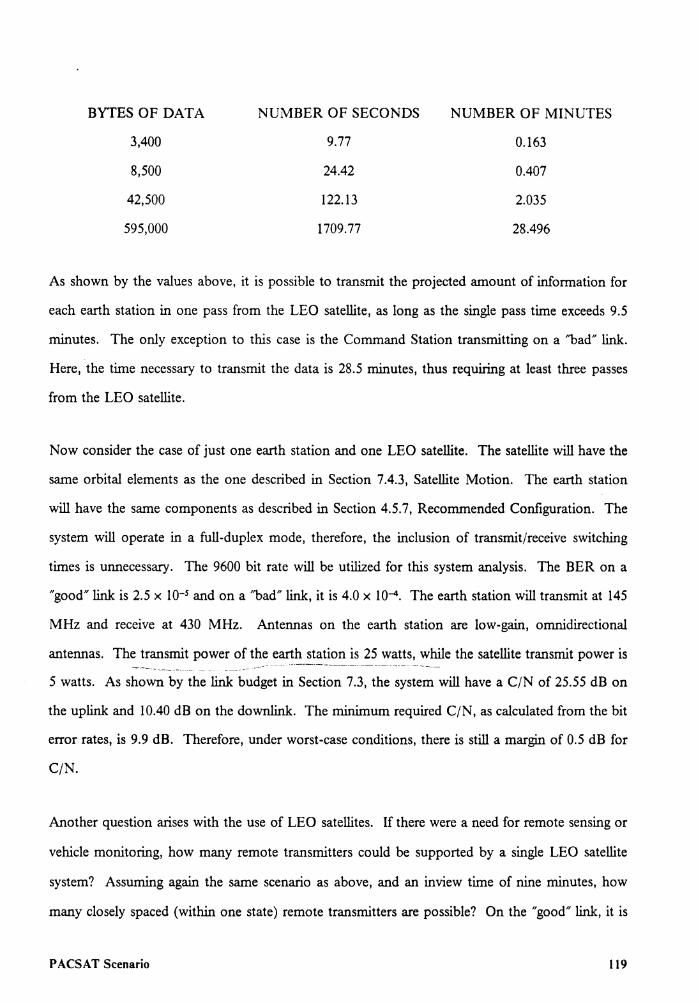
BYTES OF DATA

3,400

8,500

42,500

595,000

NUMBER OF SECONDS

9.77

24.42

122.13

1709.77

NUMBER OF MINUTES

0.163

0.407

2.035

28.496

As shown by the values above, it is possible to transmit the projected amount of information for

each earth station in one pass from the LEO satellite, as long as the single pass time exceeds 9.5

minutes. The only exception to this case is the Command Station transmitting on a 'bad" link.

Here, the time necessary to transmit the data is 28.5 minutes, thus requiring at least three passes

from the LEO satellite.

Now consider the case of just one earth station and one LEO satellite. The satellite will have the

same orbital elements as the one described in Section 7.4.3, Satellite Motion. The earth station

will have the same components as described in Section 4.5.7, Recommended Configuration. The

system will operate in a full-duplex mode, therefore, the inclusion of transmit/receive switching

times is unnecessary. The 9600 bit rate will be utilized for this system analysis. The BER on a

"good" link is 2.5 x l0-5 and on a 'bad" link, it is 4.0 x IQ-4. The earth station will transmit at 145

MHz and receive at 430 MHz. Antennas on the earth station are low-gain, omnidirectional

antennas. The transmit power of the earth station is 25 watts, while the satellite transmit power is

5 watts. As shown by the link budget in Section 7.3, the system will have a C/N of 25.55 dB on

the uplink and 10.40 dB on the downlink. The minimum required C/N, as calculated from the bit

error rates, is 9.9 dB. Therefore, under worst-case conditions, there is still a margin of 0.5 dB for

C/N.

Another question arises with the use of LEO satellites. If there were a need for remote sensing or

vehicle monitoring, how many remote transmitters could be supported by a single LEO satellite

system? Assuming again the same scenario as above, and an inview time of nine minutes, how

many closely spaced (within one state) remote transmitters are possible? On the "good" link, it is


possible to transfer 563,760 bytes of information within the nine minute window. On the "bad"

link, it is possible to transfer 187,920 bytes of information within the nine minute window. If there

were 100 remote transmitters, how much information can each transmitter upload to the satellite?

On the "good" link, each can transfer 5,637 bytes of data, and on the "bad" link, each can transfer

1,879 bytes of data. The 5,637 bytes of data corresponds to approximately 3.3 pages of information,

and the 1,879 bytes of data corresponds to approximately 1.1 pages of information. Next, how

many remote transmitters can be supported if each transmitter wishes to upload one page of

information? On the "good" link, 331 remote transmitters may be supported, while on the 'bad"

link, only 110 may be supported. Therefore, a single LEO satellite system seems to be well suited

for remote sensing and vehicle monitoring. The major disadvantage, as stated earlier, is that the

monitoring would only occur approximately every 90 minutes. So, if the user were able to adapt

to this periodic coverage, the system could operate satisfactorily.

P ACSAT Scenario 120

9.0 Conclusion

Some topics that were investigated in this thesis include the following. Low-earth-orbit satellites

can be used for many varied purposes. The main use for low-earth-orbit satellites is in the area of

stroe-and-forward communications. Among some other uses for low-earth-orbit satellits are,

remote sensing, rescue communications, vehicle location, and navigation. Low-earth-orbit

satellites, however, are not appropriate for use in a real-time communication system. As an

example, consider two earth stations separated by a distance of 2000 kilometers, they can only

communicate for approximately 5 minutes in real time; two earth stations separated by a distance

of 3000 kilometers can communicate for approximately 3 minutes in real time. A store-and-forward

system can be implemented with as few as one LEO satellite in a circular orbit at an altitude of 800

kilometers. Although there are a few different protocols available for satellite communications, the

one most popular among the amateur community for packet-radio (a store-and-forward system) is

the Amateur X.25 protocol.

This thesis also contains a conceptual design for a semi-portable, low-cost earth station. The design

includes a dual-band, full-duplex, UHF /VHF transceiver and an omnidirectional, low-gain antenna.

The uplink frequency is 145 MHz, while the downlink frequency is 430 MHz. The total cost of

such a sytem utilizing amateur radio equipment that is on the market today is approximately $6000.

This cost is for only the major components in the earth station design. The dual-band transceivers

Conclusion 121

can operate in full-duplex mode and have a bandwidth of IO to 15 kHz. The most common bit

rates that are in wide spread use in the amateur community are 1200 and 2400 bps. Although still

in an experimental stage in the amateur arena, the 9600 bps rate is becoming a more popular bit

rate to use.

The maximum Doppler shift for an 800 kilometer altitude, circular orbit satellite was concluded to

be 10158.58 Hz for a minimum earth station elevation angle often degrees. The maximum Doppler

shift rate of change is approximately 82 Hz per second.

Some other topics that are discussed in the thesis are the following. To transfer four megabytes of

satellite memory at a bit rate of 9600 bps, requires 66.96 minutes on a link with a BER of

2.5 x 10-s and 200.88 minutes on a link with a BER of 4.0 x lQ-4 • Inview generation for twenty

earth stations and seven satellites was presented. Statistical analysis of the obtained data includes

minimum inview time, maximum inview time, number of inviews, average inview time, and total

inview time for all combinations of earth stations and satellites. With text compression, there are

1700 bytes on a standard page of A4 text. A link budget was presented for a specific satellite

situation. The overall C/N for the uplink was shown to be 31.55 dB, while for the downlink, it

was shown to be 16.40 dB. A margin of 6 dB must still be included in these figures.

Areas of future work include:

• the exploration of ACE-type orbits for communication needs

• the construction of an eart4 station to work the UoSAT D satellite's PCE

• an in-depth study of the Lindenblad, the quadrifilar helix, and the turnstile-reflector array

antennas

• the analysis of different satellite constellations for the optimization of a certain "window" or

earth station site

• the use of a general purpose simulator for the simulation of a typical network of satellites and

earth stations

Conclusion 122

References

1. The American Radio Relay League, ARRL Amateur Radio Computer Networking Conferences 1-4, Pioneer Papers on Packet Radio 1981-1984, Newington, CT, 1985

2. Richard Binder, Stephen D. Huffman, Itzhak Gurantz, and Peter A. Vena, "Crosslink Architectures for a Multiple Satellite System", Proceedings of the IEEE, vol. 75, no. l, January 1987

3. Kenneth Brayer, "Packet Switching for Mobile Earth Stations via Low-Orbit Satellite Network", Proceedings of the IEEE, vol. 72, no. 11, November 1984

4. David R. Brooks, "An Introduction to Orbit Dynamics and its Application to Satellite-Based Earth Monitoring Missions", NASA Reference Publication 1009, Langley Research Center, Hampton, Virginia, November 1977

5. Martin R. Davidoff, The Satellite Experimenter's Handbook, American Radio Relay League, Newington, CT, 1985

6. Editor B. G. Evans, Satellite Communication Systems, Peter Peregrinus Limited, London, United Kingdom, 1987

7. Kamilo Feher, "Digital Communications - Satellite/Earth Station Engineering", Prentice-Hall Inc., Englewood Cliffs, New Jersey, 1983

8. Terry L. Fox, AX.25 Amateur Packet-Radio Link-Layer Protocol Version 2.0 October 1984, American Radio Relay League, Newington, CT, 1984

9. Edwin F. Harrison and Richard N. Green, "Orbit Analysis for Coastal Zone Oceanography Observations", A/AA Paper 73-207, January 10-12, 1973

10. Joseph P. Havlicek, James H. Polaha, Charles W. Bostian, and John C. McKeeman, IBM/ Virginia Tech Joint Development Project Final Report on Low-Earth-Orbit Communications Satellites, Bradley Department of Electrical Engineering, Virginia Polytechnic Institute and State University, Blacksburg, Virginia, 24061, Document Number 8/05/88, July 1, 1988

References 123

11. Stan Horzepa, Your Gateway to Packet Radio, American Radio Relay League, Newington, CT, 1988

12. "Scout Planning Guide", LTV Missiles and Electronics Group - Missiles Division, May 1987

13. James Martin, Communications Satellite Systems, Prentice-Hall Inc., Englewood Cliffs, New Jersey, 1978

14. Anthony C. Materna, "Small Low-Earth-Orbiting Payloads", A/AA Paper 82-1765

15. L. Rex Megill, Frank J. Redd, and Rex W. Ridemour, "Get Away Special Class Satellites (CANSA TS): Design Constraints, Applications, and Recent Technology Advances at Utah State University", A/AA Paper 87-0583, January 12-15, 1987

16. National Technical Information Service - U. S. Department of Commerce, Satellite Communications Reference Data Handbook, Defense Communications Agency, Virginia, July 1972

17. "Lightsat Applications for the State of Virginia", Personal correspondence from Jason O'Neil to Fred Ricci on October 24, 1987

18. Timothy Pratt and Charles W. Bostian, Satellite Communications, John Wiley and Sons, New York, 1986

19. Wilbur L. Pritchard and Joseph A. Sciulli, Satellite Communications Systems, John Wiley and Sons, New York, 1986

20. Paul L. Rinaldo, "ARRL Board Approves AX.25 Packet-Radio Link-Layer Protocol", QST, vol. 68, no. 12, December 1984

21. Andrew E. Turner and Kent M. Price, "The ACE Orbit: A New Communications Satellite Orbit", QEX, March 1989

22. "PACSAT" Revision 1.1 (March 29, 1988), Personal correspondence from Jeff W. Ward to Dr. Gary Garriott on April 8, 1988

23. L. P. Yeh, "Geostationary Satellite Orbital Geometry", IEEE Transactions on Communications, vol. COM-20, no. 2, April 1972

References 124

Bibliography

Penina Axelrad and John Kelley, "Near Earth Orbit Determination and Rendezvous Navigation using GPS", PLANS '86 - Position Location and Navigation Symposium, Las Vegas, Nevada, November 4-7, 1986

W. I. Berks and Werner Luft, "Photovoltaic Solar Arrays for Communication Satellites", Proceedings of the IEEE, vol. 59, no. 2, February 1971

G. Beutler, W. Gurtner, M. Rothacher, T. Schildknecht, and I. Bauersima, "Determination of GPS Orbits using Double Difference Carrier Phase Observations from Regional Networks", Bulletin Geodesique, vol. 60, no. 3, April 1986

V. K. Bhargava, D. Haccoun, R. Matyas, and P. Nuspl, Digital Communications by Satellite, John Wiley and Sons, New York, 1981

G. B. Bleazard, Introducing Satellite Communications, NCC Publications, The National Computing Centre Limited, Manchester, England, 1985

A. W. Boyd and A. E. Fuhs, "General Purpose Satellites: A Concept for Affordable Low Earth Orbit Vehicles", A/AA Paper 86-0584, January 15-16, 1987

Walter H. Braun and J. E. Keigler, "RCA Satellite Networks: High Technology and Low User Cost", Proceedings of the IEEE, vol. 72, no. 11, November 1984

Karen A. H. Burt, "Communications Satellite Configurations for the Future", Space Tech '86, May 1986

M. F. Catedra, "Dual-Band Antenna for Telemetry, Tracking and Control (TTC) of Satellites at KU-Band", Electronics Letters, vol. 22, no. 25, December 4, 1986

D. Chakraborty, "Constraints in KU-Band Continental Satellite Network Design", IEEE Communications Magazine, vol. 24, no. 8, August 1986

Editor Wushow Chou, Computer Communications: Volume I Principles, Prentice-Hall Inc., Englewood Cliffs, New Jersey, 1983

Robert D. Culp and Richard C. Murrow, "Minimum Altitude Variation Arcs", Society of Automotive Engineers, Pub. no. 861665, 1987

Bibliography 125

Francois Desvignes, Francois-Xavier Doittau, Jean-Pierre Krebs, and Maurice Tissot, "Optical Sensors for Spacecraft Attitude Measurement with respect to the Earth", Infrared Technology and Applications, November 26-29, 1985

Andre R. Dion and Leon J. Ricardi, "A Variable-Coverage Satellite Antenna System", Proceedings of the IEEE, vol. 59, no. 2, February 1971

Jerald F. Farrell and Carson E. Agnew, "Mobile Communications using Satellite", Space Tech '86, May 1986

Emanual Fthenakis, Manual of Satellite Communications, McGraw-Hill Book Company, New York, 1984

Robert M. Gagliard, Satellite Communications, Van Nostrand Reinhold Company, New York, 1984

P. S. Goel, K. S. Chandra. and P. Kudva, "Observer Based Design of Normal Mode Attitude Control for IRS Satellite", Space Dynamics and Celestial Mechanics, November 14-16, 1985

P. S. Goel, P. Natarajan, and P. Kudva, "Satellite Attitude Acquisition by a Momentum Bias System", Space Dynamics and Celestial Mechanics, November 14-16, 1985

Editors R. G. Gould and Y. F. Lum, "Communication Satellite Systems: An Overview of the Technology", IEEE Press, 1976

John Griffiths, Radio Wave Propagation and Antennas: An Introduction, Prentice-Hall International, New Jersey, 1987

Tri T. Ha, Digital Satellite Communications, Macmillian Publishers, New York, 1986

Editor Bruce S. Hale, The 1989 ARRL Handbook for the Radio Amateur, American Radio Relay League, Newington, CT, 1988

Editor Robert J. Halprin, The ARRL Operating Manual, American Radio Relay League, Newington, CT, 1988

Daniel J. Holt, "A Primer on Communication Satellite Design", Aerospace Engineering, June 1983

Paul S. Jorgensen, "Relativity Correction in GPS User Equipment", PLANS '86 - Position Location and Navigation Symposium, Las Vegas, Nevada, November 4-7, 1986

Robert R. Lovell and C. Louis Cuccia, "Switches, Lasers & Electronically-Hopped Beam Antennas in Space: NASA's Advanced Communications Technology Satellite", Space Tech '86, May 1986

G. Maral and M. Bousquet, Satellite Communications Systems, John Wiley and Sons, New York, 1986

Michael Menn, "Autonomous Navigation for GPS via Crosslink Ranging", PLANS '86 -Position Location and Navigation Symposium, Las Vegas, Nevada, November 4-7, 1986

K. Miya, Satellite Communications Technology, K. D. D. Inc., Japan, 1985

Editor K. Miya, Satellite Communications Engineering, Lattice Company Limited, Tokyo, Japan, 1975

Lloyd Motz and Anneta Duveen, Essentials of Astronomy, Columbia University Press, New York and Guildford, Surrey, 1977,

Bibliography 126

Office of Scientific and Technical Information, Space Flight Handbooks Volume /, Orbital Flight Handbook, Part I - Basic Techniques and Data, NASA, Washington, D.C., 1963

Stan Prentiss, Satellite Communications, Tab Books Inc., Blue Ridge Summit, Pennsylvania, 1983

S. 0. Rice, "Intervals between Periods of No Service in Certain Satellite Communication Systems - Analogy with a Traffic System", The Bell System Technical Journal, vol. 41, no. 5, 1962

J. D. Rinehart and M. F. Robbins, "Characteristics of the Service Provided by Communications Satellites in Uncontrolled Orbits", The Bell System Technical Journal, vol. 41, no. 5, 1962

A. E. Roy, Orbital Motion, Second Edition, Adam Hilger Limited, Bristol, Great Britain, 1982

A. E. Roy and D. Clarke, Astronomy: Principles and Practices, Adam Hilger Limited, Bristol, Great Britain, 1977

J. N. Slater and L. A. Trinogga, Satellite Broadcasting Systems: Planning and Design, Ellis Horwood Limited (a division of John Wiley and Sons), New York, 1985

James J. Spilker, Digital Communications by Satellite, Prentice-Hall Inc., Englewood Cliffs, New Jersey, 1977

William Stallings, Data and Computer Communications, Macmillan Publishing Company, New York, 1985

L. C. Tillotson, "A Model of a Domestic Satellite Communication System", The Bell System Technical Journal, vol. 47, no. 10, December 1968

Fouad A. Tobagi, "Multiaccess Protocols in Packet Communications Systems", IEEE Transactions on Communications, vol. 28, no. 4, April 1980

Andrew E. Turner and Kent M. Price, "The Potential in Non-Geosynchronous Orbit", Satellite Communications, June 1988

James A. Van Allen Origins of Magnetospheric Physics, Smithsonian Institute Press, Washington, D. C., 1983

H. L. VanTrees, E. V. Hoverstein, and T. P. McGarty, "Communications Satellites: Looking to the 1980's", IEEE Spectrum, vol. 14, no. 12, December 1977

John Voelcker, "Helping Computers Communicate", IEEE Spectrum, vol. 23, no. 3, March 1986

Robert Vondra, Keith Thomasson, and Albert Solbes, "A Pulsed Electric Thruster for Satellite Control", Proceedings of the IEEE, vol. 59, no. 2, February 1971

John Weissberg and Keiken Ninomiya, "Improved Method for the Initial Attitude Acquisition Maneuver", JoW7lal of Guidance, Control, and Dynamics, vol. 10, no. 3, May-June 1987

L. Wiederholt, B. Fink, G. Liu, M. May, and R. Tafel, "GPS UE Data Generator", PLANS '86 - Position Location and Navigation Symposium, Las Vegas, Nevada, November 4-7, 1986

William W. Wu, Elements of Digital Satellite Communications, Computer Science Press, Two Volumes, 1984

Bibliography 127

Appendix A. Low-Earth-Orbit Satellites in Use

A.1 GLOMR

Satellite: Global Low Orbiting Message Relay (GLOMR) Satellite

Developer: Defense Systems Incorporated (OSI)

Deployment date: October 31, 1985

Deorbit date: December 26, 1986

Mission: Packet-switched, store-and-forward communications

System costs: Less than $1,000,000

Construction Time: Less than one year

Stabilization: Unstabilized

Predicted Satellite Lifetime: Two to three years

Deployment Method: GAS CAN

Weight: 150 pounds

Size: Sixteen inch diameter multifaceted polygon

Power: Solar cells and lead acid batteries

Transmitter/Receiver: Two 10 watt transmitters, two receivers

Appendix A. Low-Earth-Orbit Satellites in Use 128

Data rate: ~~00 b.ps

Frequency Range: 290 to 400 MHz

Antennas: Omni-directinn_aLb.ro.adband array ----On-board Computer: Two systems with a total memory of 2 megabytes

A.2 NUSAT

Satellite: Northern Utah Satellite (NUSAT)

Developers:

Utah State University

Weber State College

New Mexico State University

Twenty-six companies

Deployment date: April 29, 1985

Deorbit date: December 15, 1986

Mission:

To measure antenna patterns of L-band radars involved in the world-wide air traffic

control network operated by member nations of the International Civil Aviation

Organization (ICAO)

System costs:

Approximately $20,000 (without the inclusion of donated materials)

Approximately $1,500,000 (with the inclusion of donated materials)

Construction Time: Approximately five years

Stabilization: Unstabilized

Predicted Satellite Lifetime: Eight months



Weight: 150 pounds

Size: Nineteen inch octahedron with a base nine inches in diameter

Power:

Five watts or less when averaged over an orbit

Energy storage on-board of 50 watt hours

Transmitter/Receiver:

Earth Station Transmitter - Spectrum Communications model SCT410 with a 7 W output

boosted to 100 W by an external linear power amplifier

Satellite Receiver - ICOM model IC-4AT transceiver with the transmitter section

removed; has a sensitivity of 0.35 microvolts for 20 dB noise quieting

Satellite Transmitter - modified Spectrum Communications model SCT 110 with an

output power of 10 W

Earth Station Receiver - Spectrum Communications model SCR-200

Data rate: 2400 bps

Frequency Range: 450 MHz up / 137.9 MHz down

Antennas: Q_tnni:direc_tional_broadband_array

On-board Computer:

NSC 800 National Semiconductor microcomputer; eight-bit, Z80 compatible,

microprocessor; 2 kilobytes of ROM and 2 kilobytes of RAM with the microcomputer,

and 48 kilobytes of RAM which are turned on under software control

A.3 ORION

Satellite: ORION

Developer: Naval Postgraduate School

Deployment date: 1990


Mission: Research in near-earth space, communications, miniature earth imaging, military

System costs: $1,000,000

Construction Time: N/A

Stabilization:

Active nutation control techniques employed for spin stabilization about longitudinal axis

Predicted Satellite Lifetime: Three years


Weight: Less than 250 pounds

Size: Cylindrical structure 19 inches in diameter by 35 inches in length

Power: 75 watts, with 20 watts available for the payload

Transmitter/Receiver: N/A

Data rate: 4800 bps

Frequency Range: N/A

Antennas: NI A

On-board Computer:

A.4

16 bit system microprocessor, augmented by a 12 megabyte

magnetic bubble memory data storage system

UoSAT

Satellites: UoSA T 1 (OSCAR 9) and UoSAT 2 (OSCAR 11)

Developer: The University of Surrey

Deployment date: UoSAT 1 - October 1981 UoSAT 2 - March 1984

Deorbit date: Both still in orbit

Mission [6):


• To investigate the feasibility of the design, construction, test and launch of a relatively

small, inexpensive spacecraft capable of a significant contribution to the engineering,

scientific, educational, and amateur radio communities.

• To stimulate and promote a greater awareness of and interest in space engineering and

science in the academic community by direct, active participation in the satellite

experimental program.

• To broaden the scope of the Amateur Satellite Program by catering for the interests of the

amateur scientist in addition to traditional amateur radio communications.

• To evaluate the use and performance of novel technologies, spacecraft systems

architectures and cost-effective spacecraft engineering techniques to provide a lower cost

entry level into space activities.

System costs:

UoSAT 1

$237,000 (1981 figures) (without the inclusion of donated materials)

$400,000 (1981 figures) (with the inclusion of donated materials)

UoSAT 2

$715,000 (1984 figures) (without the inclusion of donated materials)

$805,000 (1984 figures) (with the inclusion of donated materials)

NASA provided for the launch and launcher integration, which cost an additional

$500,000

Construction Time:

UoSA T 1 - Thirty months with a team of 20 members

UoSA T 2 - Seven months with a team of 35 members

Stabilization: Three axis magnetorquer coils and a gravity gradient boom

Predicted Satellite Lifetime: NI A

Deployment Method: Piggy-back mission on a DELTA 2310 launch vehicle

Weight: N/A

Size: Sixteen inch diameter multifaceted polygon


Power:

Commercial grade batteries, battery charge regulator,

power conditioning and distribution system, silicon solar cells

Transmitter/Receiver: N/A

Data rate: 1200 bps on UoSAT 1, 4800 bps on UoSAT 2

Frequency Range: 145.825 MHz up

Antennas: Omni-directional broadband array

On-board Computer:

RCA1802 with 48 kilobytes of RAM, real time clock, bootstrap loader and

communications ports and pathways

UoSAT 1 - 8 kilobytes of on-board computer memory

UoSAT 2 - 32 kilobytes of on-board computer memory


Appendix B. Sources of Packet-Radio Information

The following list of articles provide a good review of current packet-radio information.

Bill Ashby, ''The Year 2000 - Packet Radio Then and Now", 73 Magazine, August 1987, Issue #323, pages 24-25

Robert Diersing, "UoSATs: The British Connection Part I", 73 Magazine, May 1988, Issue #332, pages 20-22

Robert Diersing, "UoSATs: The British Connection Part II", 73 Magazine, June 1988, Issue #333, pages 29-31

Stan Horzepa, "Packet Radio - What's the Difference?", QST, February 1985, Vol 69, No 2, page 64

Stan Horzepa, "The Shopper's Guide to Packet-Radio TNCs", QST, March 1987, Vol 71, No 3, pages 17-21 and 44

Lyle Johnson, "Join the Packet-Radio Revolution", 73 Magazine, September 1983, Issue #276, pages 19-23

Lyle Johnson, "Join the Packet-Radio Revolution - Part II", 73 Magazine, October 1983, Issue #277, pages 20-31

Lyle Johnson, "Join the Packet-Radio Revolution - Part III", 73 Magazine, January 1984, Issue #280, pages 36-44

Marc Leavey, "Rtty Loop - Amateur Radio Teletype; Trying Harder to Be Friendly", 73 Magazine, January 1989, Issue #340, page 59

Brian Lloyd, "Packet Talk - Latest in Digital Hamming; Letters, Equalization, and Modems", 73 Magazine, March 1988, Issue #330, pages 77-78

Brian Lloyd, "Packet Talk - Latest in Digital Hamming; Packet in Emergency Communications", 73 Magazine, April 1988, Issue #331, pages 67-68

Brian Lloyd, "Packet Talk - Latest in Digital Hamming; Building a Duplex Digipeater", 73 Magazine, June 1988, Issue #333, pages 61-61

Appendix B. Sources of Packet-Radio Information 134

Andy MacAllister, "Hamsats - Amateur Radio Via Satellite; Spaceborne Bits", 73 Magazine, June 1988, Issue #333, pages 78-79

Andy MacAllister, "Hamsats - Amateur Radio Via Satellite; Hamsats a Year Older", 73 Magazine, January 1989, Issue #340, page 91

David McLanahan, "Emergency Pocket Packet: Instant Packet in your Jacket", 73 Magazine, April 1988, Issue #331, pages 25-29

Harold Price, 'What's All This Racket About Packet?", QST, July 1985, Vol 69, No 7, pages 14-17

Harold Price, "A Closer Look at Packet Radio", QST, August 1985, Vol 69, No 8, pages 17-20

Gwyn Reedy, "A Packet Primer", 73 Magazine, August 1986, Issue #311, pages 28-32

Paul Rinaldo, "ARRL Board Approves AX.25 Packet-Radio Link-Layer Protocol", QST, December 1984, Vol 68, No 12, pages 35-36

Vern Riportella, "Amateur Satellite Communications; Antennas for Working OSCAR", QST, October 1985, Vol 69, No 10, page 72

Vern Riportella, "Amateur Satellite Communications; Basic Satellite-Tracking Themes", QST, November 1985, Vol 69, No 11, page 86

Vern Riportella, "Amateur Satellite Communications; Basic Satellite-Tracking Themes", QST, December 1985, Vol 69, No 12, page 85

Vern Riportella, "Amateur Satellite Communications; On the OSCARs: Coping with Dr Doppler", QST, January 1989, Vol 73, No l, page 89-90

Steven Roberts, "Bicycle-Mobile Packeteering", 73 Magazine, April 1988, Issue #331, pages 41-42

David Summer, "It Seems to Us ... ; Packet Fever", QST, April 1986, Vol 70, No 4, page 9

David Summer, "It Seems to Us ... ; Good News for Packeteers", QST, May 1986, Vol 70, No 5, page 9

Patty Winter, "Packet Radio in Emergency Communications", QST, September 1986, Vol 70, No 9, pages 53-57

Also, the following magazines are useful in the area of amateur radio communications:

73 Magazine

Ham Radio Magazine

QST

Appendix F in [11] (pages A-27 to A-36) lists hardware and software suppliers, information, and

organizations pertinent to packet-radio.

Appendix B. Sources of Packet-Radio Information 135

Appendix C. Doppler Information

The output, as shown in Appendix C, consists of the epoch DA TE and TIME for the current line.

The azimuth (AZ) and elevation (EL) angles, in degrees, are then given for the epoch at the front

of the line. Next is LNG/LAT, the subsatellite point. This is the longitude (LNG) and latitude

(LAT) on the earth where a line connecting the satellite with the earth's center would cross the

earth's surface. RANGE and PH are the slant range and the phase. Slant range is the distance in

meters from the earth station to the satellite. Phase is the part of the orbit the satellite is in. Phase

is measured in part out of 256 of an orbit. This representation of an orbit was adopted by engineers

who were designing Phase III satellites and this type of representation is easy in eight bit computers.

0 is apogee, 128 is perigee, and 255 is one step before the next perigee. The final column is the

Doppler frequency shift (DOPPLER). It is determined by the relative velocity between the

spacecraft and the earth station.

The simulation was implemented with a twenty second time step. The data in the body of the

thesis, however, used a time step of five seconds. The orbit used for this simulation is explained

in Section 7.4.3, Satellite Motion.

Appendix C. Doppler Information 136

Date Time Az/El Lng/Lat Range/Ph Doppler 07MAR89 014136 348/ 0 93/ 63 3288/ 66 4489Hz 07MAR89 014156 350/ 1 91/ 63 3228/ 67 4228Hz 07MAR89 014216 352/ 1 88/ 63 3170/ 68 3951Hz 07MAR89 014236 354/ 2 86/ 63 3117 I 69 3657Hz 07MAR89 014256 357/ 2 83/ 62 3069/ 70 3347Hz 07MAR89 014316 359/ 3 81/ 62 3024/ 71 3021Hz 07MAR89 014336 2/ 3 79/ 62 2984/ 71 2680Hz 07MAR89 014356 5/ 3 76/ 61 2949/ 72 2324Hz 07MAR89 014416 8/ 4 74/ 61 2920/ 73 1955Hz 07MAR89 014436 10/ 4 72/ 60 2895/ 74 1575Hz 07MAR89 014456 13/ 4 70/ 60 2876/ 75 l 186Hz 07MAR89 014516 16/ 4 68/ 59 2862/ 76 789Hz 07MAR89 014536 19/ 4 66/ 58 2854/ 76 386Hz 07MAR89 014556 22/ 4 64/ 58 2851/ 77 -18Hz 07MAR89 014616 25/ 4 63/ 57 2854/ 78 -423Hz 07MAR89 014636 28/ 4 61/ 57 2863/ 79 -825Hz 07MAR89 014656 31/ 4 59/ 56 2877/ 80 -1223Hz 07MAR89 014716 33/ 4 58/ 55 2897/ 81 -1613Hz 07MAR89 014736 36/ 4 56/ 54 2922/ 82 -1994Hz 07MAR89 014756 39/ 3 55/ 54 2953/ 82 -2363Hz 07MAR89 014816 42/ 3 53/ 53 2988/ 83 -2720Hz 07MAR89 014836 44/ 3 52/ 52 3028/ 84 -3062Hz 07MAR89 014856 47/ 2 51/ 51 3073/ 85 -3390Hz 07MAR89 014916 49/ 2 49/ 50 3123/ 86 -3701Hz 07MAR89 O 14936 52/ 1 48/ 49 3177 I 87 -3996Hz 07MAR89 014956 54/ 1 47/ 49 3234/ 87 -4275Hz 07MAR89 015016 56/ 0 46/ 48 3296/ 88 -4538Hz ------------------------ END 0 F PASS ------------------------07MAR89 032443 338/ 0 101/ 61 3291/ 72 8071Hz 07MAR89 032503 339/ 1 99/ 61 3179/ 73 7995Hz 07MAR89 032523 341/ 2 97/ 60 3069/ 74 7906Hz 07MAR89 032543 342/ 3 95/ 60 2959/ 75 7803Hz 07MAR89 032603 344/ 4 93/ 59 2851/ 76 7685Hz 07MAR89 032623 345/ 6 91/ 58 2745/ 77 7549Hz 07MAR89 032643 347/ 7 89/ 58 2641/ 78 7394Hz 07MAR89 032703 349/ 8 88/ 57 2539/ 78 7215Hz 07MAR89 032723 351/ 9 86/ 56 2440/ 79 701 lHz 07MAR89 032743 353/10 84/ 56 2343/ 80 6778Hz 07MAR89 032803 356/12 83/ 55 2251/ 81 6511Hz 07MAR89 032823 359/13 81/ 54 2162/ 82 6208Hz 07MAR89 032843 1/14 80/ 53 2078/ 83 5862Hz 07MAR89 032903 5/16 78/ 53 1999/ 83 5471Hz 07MAR89 032923 8/ 17 77 / 52 1925/ 84 5029Hz 07MAR89 032943 12/18 76/ 51 1859/ 85 4534Hz 07MAR89 033003 16/19 75/ 50 1799/ 86 3984Hz 07MAR89 033023 21/21 73/ 49 1748/ 87 3379Hz 07MAR89 033043 26/22 72/ 48 1705/ 88 2721Hz 07MAR89 033103 31/22 71/ 47 1672/ 89 2016Hz 07MAR89 033123 36/23 70/ 47 1649/ 89 1274Hz 07MAR89 033143 41/23 69/ 46 1637/ 90 506Hz 07MAR89 033203 47/23 68/ 45 1635/ 91 -272Hz 07MAR89 033223 52/23 67/ 44 1644/ 92 -1044Hz 07MAR89 033243 58/22 66/ 43 1664/ 93 -1797Hz 07MAR89 033303 63/22 65/ 42 . 1694/ 94 -2516Hz 07MAR89 033323 68/21 64/ 41 1734/ 94 -3192Hz


07MAR89 033343 72/20 64/ 40 1783/ 95 -3816Hz 07MAR89 033403 77I19 63/ 39 1840/ 96 -4386Hz 07MAR89 033423 81/17 62/ 38 1905/ 97 -4901Hz 07MAR89 033443 84/16 61/ 37 1977/ 98 -5362Hz 07MAR89 033503 88/ l 5 60/ 36 2054/ 99 -5772Hz 07MAR89 033523 91/13 60/ 35 2137/100 -6135Hz 07MAR89 033543 93/12 59/ 34 2225/ 100 -6454Hz 07MAR89 033603 96/11 58/ 33 2317/101 -6735Hz 07MAR89 033623 98/ 9 58/ 32 2413/102 -6981Hz 07MAR89 033643 100/ 8 57/ 31 2512/103 -7197Hz 07MAR89 033703 102/ 7 56/ 30 2614/104 -7387Hz 07MAR89 033723 104/ 6 56/ 29 2718/105 -7552Hz 07MAR89 033743 106/ 4 55/ 28 2824/106 -7697Hz 07MAR89 033803 107/ 3 55/ 27 2932/106 -7823Hz 07MAR89 033823 109/ 2 54/ 26 3042/107 -7933Hz 07MAR89 033843 110/ 1 53/ 25 3153/ 108 -8029Hz 07MAR89 033903 111/ 0 53/ 24 3266/ 109 -8l13Hz ------------------------ END 0 F PASS ------------------------07MAR89 050823 323/ 0 110/ 56 3275/ 80 9120Hz 07MAR89 050843 322/ 1 108/ 55 3148/ 81 9108Hz 07MAR89 050903 322/ 3 107/ 54 3021/ 82 9089Hz 07MAR89 050923 321/ 4 105/ 53 2895/ 83 9065Hz 07MAR89 050943 321/ 5 104/ 53 2769/ 83 9033Hz 07MAR89 051003 320/ 7 103/ 52 2643/ 84 8992Hz 07MAR89 051023 320/ 8 101/ 51 2518/ 85 8941Hz 07MAR89 051043 319/10 100/ 50 2394/ 86 8878Hz 07MAR89 051103 318/11 99/ 49 2270/ 87 8800Hz 07MAR89 051123 317/13 98/ 48 2148/ 88 8705Hz 07MAR89 051143 316/15 97/ 48 2028/ 88 8588Hz 07MAR89 051203 315/17 96/ 47 1909/ 89 8445Hz 07MAR89 051223 314/20 95/ 46 1792/ 90 8268Hz 07MAR89 051243 312/22 94/ 45 1679/ 91 8051Hz 07MAR89 051303 310/25 93/ 44 1568/ 92 7781Hz 07MAR89 051323 308/28 92/ 43 1462/ 93 7446Hz 07MAR89 051343 305/31 91/ 42 1361/ 94 7028Hz 07MAR89 051403 301/35 90/ 41 1266/ 94 6505Hz 07MAR89 051423 297/39 89/ 40 1180/ 95 5855Hz 07MAR89 051443 291/43 88/ 39 1104/ 96 5053Hz 07MAR89 051503 283/47 87/ 38 1040/ 97 4081Hz 07MAR89 051523 273/51 87/ 37 991/ 98 2936Hz 07MAR89 051543 260/54 86/ 36 959/ 99 1640Hz 07MAR89 051603 245/55 85/ 35 946/ 99 248Hz 07MAR89 051623 230/55 84/ 34 952/100 -1159Hz 07MAR89 051643 216/52 84/ 33 977/101 -2496Hz 07MAR89 051703 205/49 83/ 32 1021/102 -3698Hz 07MAR89 051723 197/44 82/ 31 1080/103 -4732Hz 07MAR89 051743 190/40 82/ 30 1152/104 -5592Hz 07MAR89 051803 185/36 81/ 29 1235/105 -6292Hz 07MAR89 051823 181/32 81/ 28 1327/105 -6856Hz 07MAR89 051843 178/29 80/ 27 1426/ 106 -7308Hz 07MAR89 051903 175/26 79/ 26 1530/ 107 -7670Hz 07MAR89 051923 173/23 79/ 25 1639/108 -7961Hz 07MAR89 051943 171/20 78/ 24 1752/109 -8195Hz 07MAR89 052003 170/18 78/ 23 1868/ 110 -8385Hz 07MAR89 052023 169/16 77/ 22 1986/111 -8538Hz 07MAR89 052043 168/14 77/ 21 2106/111 -8664Hz


07MAR89 052103 167/12 76/ 20 2227/112 -8766Hz 07MAR89 052123 166/ 10 76/ 19 2350/ 113 -8849Hz 07MAR89 052143 165/ 8 75/ 18 2474/114 -8917Hz 07MAR89 052203 164/ 7 75/ 17 2599/115 -8971Hz 07MAR89 052223 164/ 5 74/ 16 2724/116 -9015Hz 07MAR89 052243 163/ 4 74/ 14 2850/116 -9050Hz 07MAR89 052303 163/ 3 73/ 13 2976/117 -9077Hz 07MAR89 052323 162/ 2 73/ 12 3103/118 -9097Hz 07MAR89 052343 162/ 0 72/ ll 3230/119 -9111Hz ------------------------ END OF PASS ------------------------07MAR89 065451 289/ 0 115/ 41 3263/ 95 4641Hz 07MAR89 065511 286/ 1 114/ 40 3200/ 95 4345Hz 07MAR89 065531 284/ l 113/ 39 3142/ 96 4030Hz 07MAR89 065551 282/ 2 113/ 38 3088/ 97 3696Hz 07MAR89 065611 279/ 2 112/ 37 3039/ 98 3344Hz 07MAR89 065631 277/3 111/36 2995/99 2975Hz 07MAR89 065651 274/3 110/35 2956/100 2588Hz 07MAR89 065711 271/ 4 110/ 34 2923/101 2187Hz 07MAR89 065731 268/ 4 109/ 33 2895/101 1772Hz 07MAR89 065751 266/ 4 108/ 32 2873/ 102 l346Hz 07MAR89 065811 263/ 4 108/ 31 2857/103 912Hz 07MAR89 065831 260/ 4 107/ 30 2848/104 471Hz 07MAR89 065851 257/ 4 107/ 29 2844/105 28Hz 07MAR89 065911 254/ 4 106/ 28 2847/106 -415Hz 07MAR89 065931 251 / 4 l 05/ 27 2856/ l 06 -855Hz 07MAR89 065951 248/ 4 105/ 26 2871/107 -l289Hz 07MAR89 070011 245/ 4 104/ 25 2892/108 -l713Hz 07MAR89 070031 243/ 3 104/ 24 2919/109 -2126Hz 07MAR89 070051 240/ 3 103/ 23 2951/ 110 -2526Hz 07MAR89 070111 237/ 3 103/ 22 2989/111 -2910Hz 07MAR89 070131 235/ 2 102/ 21 3032/112 -3277Hz 07MAR89 070151 232/ 2 101/ 19 3080/112 -3627Hz 07MAR89 070211 230/ 1 101/ 18 3133/113 -3957Hz 07MAR89 070231 227/ 1 100/ 17 3190/114 -4269Hz 07MAR89 070251 225/ 0 100/ 16 3252/115 -4562Hz ------------------------ END 0 F PASS ------------------------07MAR89 180553 165/ 0 74/ 11 3257/ 9 7518Hz 07MAR89 180613 164/ 1 73/ 12 3153/ 9 7383Hz 07MAR89 180633 162/ 2 73/ 13 3051/ 10 7232Hz 07MAR89 180653 160/ 3 72/ 14 2951/ 11 7061Hz 07MAR89 180713 159/ 4 72/ 15 2854/ 12 6869Hz 07MAR89 180733 157/ 5 71/ 16 2760/ 13 6653Hz 07MAR89 180753 154/ 6 71/ 17 2669/ 14 6411Hz 07MAR89 180813 152/ 7 70/ 18 2581/ 14 6141Hz 07MAR89 180833 150/ 8 70/ 19 2498/ 15 5839Hz 07MAR89 180853 147/ 9 69/ 20 2418/ 16 5504Hz 07MAR89 180913 144/10 69/ 21 2344/ 17 5132Hz 07MAR89 180933 141/ l 1 68/ 22 2276/ 18 4723Hz 07MAR89 180953 138/12 68/ 23 2213/ 19 4274Hz 07MAR89 181013 134/13 67/ 24 2157/ 20 3785Hz 07MAR89 181033 131/14 67/ 25 2107/ 20 3256Hz 07MAR89 181053 127/14 66/ 26 2066/ 21 2691Hz 07MAR89 181113 123/15 65/ 27 2033/ 22 2093Hz 07MAR89 181133 119/15 65/ 29 2008/ 23 1468Hz 07MAR89 181153 114/16 64/ 30 1992/ 24 822Hz 07MAR89 181213 110/16 64/ 31 1985/ 25 164Hz


07MAR89 181233 106/16 63/ 32 1987/ 25 -496Hz 07MAR89 181253 101/16 62/ 33 1999/ 26 -1150Hz 07MAR89 181313 97/15 62/ 34 2019/ 27 -1788Hz 07MAR89 181333 93/15 61/ 35 2048/ 28 -2402Hz 07MAR89 181353 89/14 60/ 36 2086/ 29 -2987Hz 07MAR89 181413 85/13 59/ 37 2131/ 30 -3536Hz 07MAR89 181433 82/13 59/ 38 2184/ 31 -4048Hz 07MAR89 181453 78/12 58/ 39 2244/ 31 -4520Hz 07MAR89 181513 75/11 57/ 40 2310/ 32 -4953Hz 07MAR89 181533 72/10 56i 40 2382/ 33 -5347Hz 07MAR89 181553 69/ 9 55/ 41 2459/ 34 -5703Hz 07MAR89 181613 67/ 8 55/ 42 2541/ 35 -6025Hz 07MAR89 181633 64/ 7 54/ 43 2627/ 36 -6314Hz 07MAR89 181653 62/ 6 53/ 44 2717/ 36 -6573Hz 07MAR89 181713 60/ 5 52/ 45 2810/ 37 -6805Hz 07MAR89 181733 58/ 4 51/ 46 2907/ 38 -7012Hz 07MAR89 181753 56/ 3 50/ 47 3006/ 39 -7197Hz 07MAR89 181813 55/ 2 49/ 48 3107/ 40 -7361Hz 07MAR89 181833 53/ 1 47/ 49 3211/ 41 -7507Hz 07MAR89 181853 52/-0 46/ 50 3317/ 42 -7637Hz ------------------------ END OF PASS ------------------------07MAR89 194753 218/ O 97/ 15 3229/ 12 9156Hz 07MAR89 194813 219/ 2 97/ 16 3102/ 13 9147Hz 07MAR89 194833 219/ 3 96/ 17 2974/ 14 9134Hz 07MAR89 194853 219/ 4 96/ 18 2847/ 14 9114Hz 07MAR89 194913 220/ 6 95/ 19 2720/ 15 9088Hz 07MAR89 194933 220/ 7 95/ 20 2593/ 16 9054Hz 07MAR89 194953 221/ 9 94/ 21 2467/ 17 9010Hz 07MAR89 195013 221/10 94/ 22 2342/ 18 8956Hz 07MAR89 195033 222/12 93/ 23 2218/ 19 8889Hz 07MAR89 195053 223/14 93/ 24 2094/ 19 8805Hz 07MAR89 195113 223/16 92/ 25 1972/ 20 8701Hz 07MAR89 195133 224/18 91/ 26 1852/ 21 8573Hz 07MAR89 195153 225/21 91/ 27 1733/ 22 8413Hz 07MAR89 195213 227/23 90/ 28 1617/ 23 8214Hz 07MAR89 195233 228/26 90/ 29 1505/ 24 7964Hz 07MAR89 195253 230/30 89/ 30 1396/ 25 7649Hz 07MAR89 195313 232/34 88/ 31 1292/ 25 7249Hz 07MAR89 195333 235/38 88/ 32 1194/ 26 6740Hz 07MAR89 195353 239/43 87/ 33 1104/ 27 6094Hz 07MAR89 195413 244/48 86/ 34 1025/ 28 5278Hz 07MAR89 195433 251/54 86/ 35 958/ 29 4265Hz 07MAR89 195453 262/60 85/ 36 907/ 30 3046Hz 07MAR89 195513 279/65 84/ 37 874/ 30 1645Hz 07MAR89 195533 302/67 83/ 38 862/ 31 130Hz 07MAR89 195553 325/65 83/ 39 870/ 32 -1393Hz 07MAR89 195613 343/61 82/ 40 900/ 33 -2818Hz 07MAR89 195633 355/55 81/ 41 948/ 34 -4070Hz 07MAR89 195653 3/50 80/ 42 1012/ 35 -5116Hz 07MAR89 195713 9/44 79/ 43 1090/ 36 -5962Hz 07MAR89 195733 13/39 78/ 44 1178/ 36 -6633Hz 07MAR89 195753 16/35 77/ 45 1274/ 37 -7161Hz 07MAR89 195813 18/31 76/ 46 1377/ 38 -7576Hz 07MAR89 195833 20/27 75/ 47 1485/ 39 -7903Hz 07MAR89 195853 21/24 74/ 48 1597/ 40 -8161Hz 07MAR89 195913 23/21 73/ 49 1713/ 41 -8367Hz


07MAR89 195933 24/19 72/ 50 1830/ 42 -8531Hz 07MAR89 195953 25/17 71/ 50 1950/ 42 -8663Hz 07MAR89 200013 25/14 69/ 51 2072/ 43 -8769Hz 07MAR89 200033 26/13 68/ 52 2195/ 44 -8854Hz 07MAR89 200053 27/11 67/ 53 2319/ 45 -8923Hz 07MAR89 200113 27 I 9 65/ 54 2443/ 46 -8978Hz 07MAR89 200133 28/ 8 64/ 54 2569/ 47 -9021Hz 07:'vlAR89 200153 28/ 6 62/ 55 2695/ 47 -9056Hz 07MAR89 200213 29/ 5 61/ 56 2821/ 48 -9082Hz 07MAR89 200233 29/ 3 59/ 57 2948/ 49 -9101Hz 07MAR89 200253 30/ 2 57/ 57 3075/ 50 -9114Hz 07MAR89 200313 30/ 1 56/ 58 3202/ 51 -9123Hz 07MAR89 200333 30/-0 54/ 59 3330/ 52 -9126Hz ------------------------ END 0 F PASS ------------------------07MAR89 213411 270/ 0 113/ 32 3288/ 26 6872Hz 07MAR89 213431 r''.1 1 113/ 33 3193/ 27 6713Hz 07MAR89 213451 27.J. 2 112/ 34 3101/ 28 6538Hz 07MAR89 213511 275/ 3 111/ 35 3011/ 29 6343Hz 07MAR89 213531 277/ 4 111/ 36 2924/ 29 6128Hz 07MAR89 213551 280/ 4 110/ 37 2840/ 30 5892Hz 07MAR89 213611 282/ 5 109/ 38 2760/ 31 5631Hz 07MAR89 213631 284/ 6 108/ 39 2683/ 32 53461-Iz 07MAR89 213651 287/ 7 107/ 40 2611/ 33 5034Hz 07MAR89 213711 290/ 8 107/ 41 2543/ 34 4694Hz 07MAR89 213731 293/ 9 106/ 42 2480/ 35 4325Hz 07MAR89 213751 296/ 9 105/ 43 2423/ 35 3926Hz 07MAR89 213811 299/10 104/ 44 2371/ 36 3499Hz 07MAR89 213831 302/11 103/ 45 2325/ 37 3043Hz 07MAR89 213851 306/ 11 102/ 46 2286/ 38 2560Hz 07MAR89 213911 309/12 101/ 47 2254/ 39 2054Hz 07MAR89 213931 313/12 100/ 48 2229/ 40 1528Hz 07MAR89 213951 317/12 99/ 49 2211/ 41 986Hz 07MAR89 214011 321/12 97/ 49 2202/ 41 434Hz 07MAR89 214031 324/12 96/ 50 2199/ 42 -123Hz 07MAR89 214051 328/12 95/ 51 2205/ 43 -678Hz 07MAR89 214111 332/12 94/ 52 2218/ 44 -1225Hz 07MAR89 214131 336/12 92/ 53 2239/ 45 -1759Hz 07MAR89 214151 339/12 91/ 54 2267/ 46 -2275Hz 07MAR89 214211 343/ 11 90/ 54 2302/ 46 -2768Hz 07MAR89 214231 346/10 88/ 55 2344/ 47 -3236Hz 07MAR89 214251 350/10 86/ 56 2393/ 48 -3676Hz 07MAR89 214311 353/ 9 85/ 57 2447/ 49 -4087Hz 07MAR89 214331 356/ 8 83/ 57 2506/ 50 -4469Hz 07MAR89 214351 359/ 8 81/ 58 2571/ 51 -4821Hz 07MAR89 214411 1/ 7 79/ 58 2641/ 52 -5145Hz 07MAR89 214431 4/ 6 78/ 59 2715/ 52 -5441Hz 07MAR89 214451 6/ 5 76/ 60 2792/ 53 -571 lHz 07MAR89 214511 9/ 4 74/ 60 2874/ 54 -5957Hz 07MAR89 214531 11/ 3 71/ 61 2958/ 55 -6180Hz 07MAR89 214551 13/ 2 69/ 61 3046/ 56 -6381Hz 07MAR89 214611 15/ 2 67/ 62 3136/ 57 -6563Hz 07MAR89 214631 16/ 1 65/ 62 3229/ 57 -6727Hz 07MAR89 214651 18/-0 62/ 62 3324/ 58 -6875Hz ------------------------ END OF PASS ------------------------07MAR89 232409 326/ 0 109/ 57 3311/ 50 3105Hz 07MAR89 232429 328/ 0 107/ 58 3270/ 51 2805Hz


07MAR89 232449 331/ 1 105/ 58 3233/ 51 2492Hz 07MAR89 232509 333/ 1 103/ 59 3200/ 52 2169Hz 07MAR89 232529 336/ 1 101/ 60 3172/ 53 1835Hz 07MAR89 232549 338/ 1 99/ 60 3149/ 54 l493Hz 07MAR89 232609 341/ 2 97/ 61 3131/ 55 1143Hz 07MAR89 232629 344/ 2 95/ 61 3117/ 56 788Hz 07MAR89 232649 346/ 2 93/ 62 3109/ 56 429Hz 07MAR89 232709 349/ 2 91/ 62 3105/ 57 67Hz 07MAR89 232729 351/ 2 88/ 62 3107/ 58 -294Hz 07MAR89 232749 354/ 2 86/ 63 3114/ 59 -654Hz 07MAR89 232809 357/ 2 83/ 63 3125/ 60 -1011Hz 07MAR89 232829 359/ 2 81/ 63 3142/ 61 -13621-Iz 07MAR89 232849 2/ I 78/ 63 3163/ 62 -1707Hz 07MAR89 232909 5/ I 76/ 63 3189/ 62 -20431-Iz 07MAR89 232929 7 / 1 73/ 63 3220/ 63 -2369Hz 07MAR89 232949 10/ 0 71/ 63 3255/ 64 -2684Hz 07MAR89 233009 12/ 0 68/ 63 3295/ 65 -2988Hz ------------------------ END OF PASS ------------------------08MAR89 011058 348/ 0 93/ 63 3296/ 65 3940Hz 08MAR89 011118 350/ 1 90/ 63 3243/ 66 3662Hz 08MAR89 011138 353/ 1 88/ 63 3194/ 67 3369Hz 08MAR89 011158 355/ 1 85/ 63 3149/ 68 3061Hz 08MAR89 011218 358/ 2 83/ 63 3109/ 69 2739Hz 08MAR89 011238 0/ 2 80/ 62 3073/ 69 2404Hz 08MAR89 011258 3/ 2 78/ 62 3042/ 70 2057Hz 08MAR89 011318 5/ 3 76/ 62 3016/ 71 1699Hz 08MAR89 011338 8/ 3 73/ 61 2995/ 72 1331 Hz 08MAR89 011358 11/ 3 71/ 61 2979/ 73 956Hz 08MAR89 011418 14/ 3 69/ 60 2968/ 74 576Hz 08MAR89 011438 16/ 3 67/ 60 2963/ 75 191Hz 08MAR89 011458 19/ 3 65/ 59 2963/ 75 -194Hz 08MAR89 011518 22/ 3 63/ 59 2968/ 76 -578Hz 08MAR89 011538 25/ 3 61/ 58 2979/ 77 -960Hz 08MAR89 011558 28/3 59/57 2995/78 -1336Hz 08MAR89 011618 30/ 3 58/ 57 3016/ 79 -1704Hz 08MAR89 011638 33/ 2 56/ 56 3042/ 80 -2064Hz 08MAR89 011658 36/ 2 54/ 55 3073/ 80 -2413Hz 08MAR89 011718 38/ 2 53/ 55 3109/ 81 -2750Hz 08MAR89 011738 41/ l 51/ 54 3150/ 82 -3074Hz 08MAR89 011758 43/ l 50/ 53 3195/ 83 -3384Hz 08MAR89 011818 46/ l 49/ 52 3244/ 84 -3679Hz 08MAR89 011838 48/ 0 47/ 51 3298/ 85 -3960Hz ------------------------ END 0 F PASS ------------------------08MAR89 025409 340/ 0 100/ 62 3297/ 72 7669Hz 08MAR89 025429 341/ 1 98/ 61 3190/ 72 7566Hz 08MAR89 025449 343/ 2 96/ 61 3086/ 73 7449Hz 08MAR89 025509 344/ 3 94/ 60 2983/ 74 73 l 7Hz 08MAR89 025529 346/ 4 92/ 60 2882/ 75 7167Hz 08MAR89 025549 348/ 5 90/ 59 2783/ 76 6997Hz 08MAR89 025609 350/ 6 88/ 58 2687/ 77 6806Hz 08MAR89 025629 352/ 7 86/ 58 2593/ 77 6590Hz 08MAR89 025649 354/ 8 84/ 57 2503/ 78 6347Hz 08MAR89 025709 357/ 9 82/ 56 2416/ 79 6073Hz 08MAR89 025729 359/ l l 81/ 56 2334/ 80 5767Hz 08MAR89 025749 2/12 79/ 55 2256/ 81 5424Hz 08MAR89 025809 5/ 13 78/ 54 2183/ 82 5043Hz


08MAR89 025829 9/14 76/ 53 2115/83 4621Hz 08MAR89 025849 12/ 15 75/ 53 2054/ 83 4156Hz 08MAR89 025909 16/ 16 73/ 52 2000/ 84 3648Hz 08MAR89 025929 20/17 72/ 51 1953/ 85 3098Hz 08MAR89 025949 24/17 71/ 50 1913/ 86 2509Hz 08MAR89 030009 29/18 70/ 49 1883/ 87 1885Hz 08MAR89 030029 33/ 18 69/ 48 1861/ 88 1234Hz 08MAR89 030049 38/ 18 68/ 48 1849/ 88 563Hz 08MAR89 030109 43/ 19 66/ 47 1845/ 89 -117Hz 08MAR89 030129 48/18 65/ 46 1852/ 90 -795Hz 08MAR89 030149 52/ 18 64/ 45 1868/ 91 -1461Hz 08MAR89 030209 57/ 18 63/ 44 1892/ 92 -2105Hz 08MAR89 030229 61/ l 7 63/ 43 1926/ 93 -2720Hz 08MAR89 030249 65/16 62/ 42 1968/ 94 -3299Hz 08MAR89 030309 69/15 61/ 41 2018/ 94 -3838Hz 08MAR89 030329 73/14 60/ 40 2075/ 95 -4335Hz 08MAR89 030349 76/13 59/ 39 2139/ 96 -4789Hz 08MAR89 030409 80/12 58/ 38 2208/ 97 -5201Hz 08MAR89 030429 83/11 58/ 37 2283/ 98 -5572Hz 08MAR89 030449 86/ 10 57/ 36 2364/ 99 -5906Hz 08MAR89 030509 88/ 9 56/ 35 2448/ 99 -6205Hz 08MAR89 030529 91/ 8 55/ 34 2536/100 -6471Hz 08MAR89 030549 93/ 7 55/ 33 2628/101 -6709Hz 08MAR89 030609 95/ 6 54/ 32 2723/ 102 -6920Hz 08MAR89 030629 97/ 5 53/ 31 2821/103 -7107Hz 08MAR89 030649 99/ 3 53/ 30 2921/104 -7273Hz 08MAR89 030709 100/ 2 52/ 29 3024/ 105 -7420Hz 08MAR89 030729 102/ 1 51/ 28 3128/105 -7551Hz 08MAR89 030749 103/ 0 51/ 27 3234/106 -7666Hz -----··················· END 0 F PASS ·············•••··•···•· 08MAR89 043742 325/ 0 109/ 57 3275/ 79 9200Hz 08MAR89 043802 325/ 1 107/ 56 3147/ 80 9197Hz 08MAR89 043822 325/ 3 105/ 55 3018/ 80 9189Hz 08MAR89 043842 325/ 4 104/ 55 2890/ 81 9175Hz 08MAR89 043902 325/ 5 102/ 54 2763/ 82 9156Hz 08MAR89 043922 325/ 7 101/ 53 2635/ 83 9130Hz 08MAR89 043942 325/ 8 100/ 52 2508/ 84 9096Hz 08MAR89 044002 324/10 98/ 51 2382/ 85 9052Hz 08MAR89 044022 324/12 97/ 51 2256/ 86 8996Hz 08MAR89 044042 324/ 14 96/ 50 2131/ 86 8926Hz 08MAR89 044102 323/16 95/ 49 2007/ 87 8839Hz 08MAR89 044122 323/18 93/ 48 1884/ 88 8729Hz 08MAR89 044142 322/20 92/ 47 1764/ 89 8593Hz 08MAR89 044202 322/23 91/ 46 1645/ 90 8421Hz 08MAR89 044222 321/26 90/ 45 1529/ 91 8205Hz 08MAR89 044242 320/29 89/ 44 1416/ 91 7931Hz 08MAR89 044302 319/33 88/ 43 1308/ 92 7580Hz 08MAR89 044322 317 /38 88/ 42 1205/ 93 7129Hz 08MAR89 044342 315/43 87/ 41 1110/ 94 6548Hz 08MAR89 044402 312/49 86/ 41 1024/ 95 5803Hz 08MAR89 044422 307/55 85/ 40 949/ 96 4857Hz 08MAR89 044442 299/62 84/ 39 889/ 97 3684Hz 08MAR89 044502 284/69 83/ 38 847/ 97 2292Hz 08MAR89 044522 257/74 83/ 37 826/ 98 734Hz 08MAR89 044542 219/74 82/ 36 827/ 99 -881Hz 08MAR89 044602 194/69 81/ 35 850/ 100 -2428Hz


08MAR89 044622 180/61 80/ 34 894/101 -3802Hz 08MAR89 044642 173/54 80/ 33 955/102 -4953Hz 08MAR89 044702 168/48 79/ 32 1031/102 -5880Hz 08MAR89 044722 165/42 78/ 31 1118/103 -6610Hz 08MAR89 044742 163/37 78/ 30 1215/104 -7177Hz 08MAR89 044802 162/ 33 77 I 29 1318/105 -76 l 8Hz 08MAR89 044822 160/29 77/ 28 1427/106 -7962Hz 08MAR89 044842 159/25 76/ 27 1540/107 -8231Hz 08MAR89 044902 159.i22 75i 25 1656/108 -8443Hz 08MAR89 044922 158/20 75/ 24 1775/108 -8611Hz 08MAR89 044942 157/ 17 74/ 23 1896/109 -8746Hz 08MAR89 045002 157/15 74/ 22 2019/110 -8853Hz 08MAR89 045022 156/13 73/ 21 2143/111 -8939Hz 08MAR89 045042 156/11 73/ 20 2268/112 -9008Hz 08MAR89 045102 156/ 9 72/ 19 2394/113 -9063Hz 08MAR89 045122 156/ 8 72/ 18 2521/113 -9106Hz 08MAR89 045142 155/ 6 71/ 17 2648/114 -9140Hz 08MAR89 045202 155/ 5 71/ 16 2775/115 -9166Hz 08MAR89 045222 155/ 4 70/ 15 2903/116 -9185Hz 08MAR89 045242 155/ 2 70/ 14 3032/117 -9198Hz 08MAR89 045302 155/ l 69/ 13 3160/118 -9206Hz 08MAR89 045322 154/-0 69/ 12 3288/119 -9210Hz ------------------------ END OF PASS ------------------------08MAR89 062308 298/ 0 116/ 45 3306/ 91 6 l l 8Hz 08MAR89 062328 296/ l 115/ 44 3222/ 92 5895Hz 08MAR89 062348 294/ l 114/ 43 3141/ 92 5651Hz 08MAR89 062408 292/ 2 113/ 42 3064/ 93 5387Hz 08MAR89 062428 290/ 3 112/ 41 2991/ 94 5100Hz 08MAR89 062458 286/ 4 111/ 40 2889/ 95 4626Hz 08MAR89 062518 284/ 5 110/ 39 2827 / 96 4280Hz 08MAR89 062538 281/ 5 109/ 38 2770/ 97 3910Hz 08MAR89 062558 278/ 6 108/ 37 2718/ 98 3516Hz 08MAR89 062618 275/ 6 108/ 36 2672/ 99 3100Hz 08MAR89 062638 272/ 7 107/ 35 2632/100 2661Hz 08MAR89 062658 269/ 7 106/ 34 2598/101 2203Hz 08MAR89 062718 266/ 7 105/ 33 2571/101 1728Hz 08MAR89 062738 263/ 8 105/ 32 2550/102 1238Hz 08MAR89 062758 260/ 8 104/ 31 2536/103 739Hz 08MAR89 062818 256/ 8 103/ 30 2529/104 233Hz 08MAR89 062838 253/ 8 103/ 29 2530/105 -274Hz 08MAR89 062858 250/ 8 102/ 28 2537/106 -778Hz 08MAR89 062918 246/ 8 102/ 27 2551/106 -1275Hz 08MAR89 062938 243/ 7 101/ 26 2573/107 -1762Hz 08MAR89 062958 240/ 7 101/ 25 2600/108 -2233Hz 08MAR89 063018 237/ 7 100/ 24 2635/109 -2686Hz 08MAR89 063038 234/ 6 99/ 23 2675/110 -3120Hz 08MAR89 063058 231/ 6 99/ 22 2722/111 -3530Hz 08MAR89 063118 228/ 5 98/ 21 2774/112 -3918Hz 08MAR89 063138 226/ 4 98/ 20 2831/112 -4281Hz 08MAR89 063158 223/ 4 97/ 18 2893/113 -4620Hz 08MAR89 063218 221/3 97/17 2959/114 -4935Hz 08MAR89 063238 218/ 2 96/ 16 3030/115 -5227Hz 08MAR89 063258 216/ 2 96/ 15 3105/116 -5495Hz 08MAR89 063318 214/ 1 95/ 14 3184/117 -5743Hz 08MAR89 063338 212/ 0 95/ 13 3265/117 -5969Hz ------------------------ END 0 F PASS ------------------------


Appendix D. Actual Inview Times

This appendix contains the actual inview times for the seven satellites and the twenty earth stations.

For the actual orbital elements of the seven satellites, refer to Table 8 on page 66.

Appendix D. Actual lnview Times 145

Satellite # 1 1:07:12 - 1:18:06 2:51:10 - 3:01:47 4:34:41 - 4:45:43 6: 17:05 - 6:25:59

11:12:05 - 11:20:49 12:52: 11 - 13:03: 11 14:36:03 - 14:46:40 16:19:45 - 16:30:47 18:02:14 - 18:11:38 19:45:28 - 19:46:21 22:57:49 - 23:05:59

Satellite #4 4:28:49 - 4:37:54 6:09: 17 - 6:20: 17 7:53:16 - 8:03:51 9:36:52 - 9:47:52

11:19:16 - 11:28:25 16:14:31 - 16:23:02 17:54:22 - 18:05:22 19:38:10 - 19:48:46 21:21:56 - 21:32:56 23:04:25 - 23: 14:00


Norfolk, Virginia

Satellite #2 1:07:12 - 1:16:24 2:47:49 - 2:58:51 4:31 :52 - 4:42:27 6: 15:25 - 6:26:25 7:57:48 - 8:06:47

12:52:53 - 13:01:34 14:32:54 - 14:43:56 16:16:45 - 16:27:22 18:00:28 - 18: 11 :29 19:42:58 - 19:52:25 21:26:00 - 21:27:25

Satellite #5 1:14:52 - 1:23:32 6:09:39 - 6:18:37 7:49:59 - 8:01:00 9:33:57 - 9:44:34

11:17:35 - 11:28:37 13:00:00 - 13:09:13 17:55:22 - 18:03:46 19:35:06 - 19:46:06 21:18:51 - 21:29:28 23:02:38 - 23: 13:38

Satellite #7 1:10:27 - 1:21:05 2:53:57 - 3:04:59 4:36:20 - 4:45: 10 9:31: 15 - 9:40:05

11:11:27 - 11:22:27 12:55:22 - 13:05:59 14:39:02 - 14:50:02 16:21:29 - 16:30:50 21:17:00 - 21:25:15 22:56:35 - 23:07:34

Satellite #3 2:48:01 - 2:57:10 4:28:32 - 4:39:34 6: 12:33 - 6:23:09 7:56:08 - 8:07:09 9:38:33 - 9:47:35

14:33:42 - 14:42: 18 16: 13:38 - 16:24:38 17:57:28 - 18:08:05 19:41:13 - 19:52:12 21:23:41 - 21:33:13 23:06:35 - 23:08:26

Satellite #6 1:12:59 - 1:24:00 2:55:26 - 3:04:41 7:50:51 - 7:59: 11 9:30:31 - 9:41 :31

11:14:15 - 11:24:52 12:58:04 - 13:09:02 14:40:35 - 14:50:17 16:23:16 - 16:25:57 19:36:39 - 19:44: 19 21:15:43 - 21:26:36 22:59:08 - 23:09:48

146

Satellite # 1 1:12:59 - 1:24:00 2:55:26 - 3:04:41 7:50:51 - 7:59: 11 9:30:31 - 9:41:31

11:14:15 - 11:24:52 12:58:04 - 13:09:02 14:40:35 - 14:50: 17 16:23:16 - 16:25:57 19:36:39 - 19:44: 19 21:15:43 - 21:26:36 22:59:08 - 23:09:48

Satellite #4 1:16:17 - 1:17:25 2:53:15- 2:56:07 4:29:04 - 4:38: 17 6:09:35 - 6:20:36 7:53:14 - 8:03:59 9:36:37 - 9:47:37

11:18:55 - 11:28:06 13:01:07 - 13:03:51 14:39:38 - 14:41:00 16:14:42 - 16:23:26 17:54:41 - 18:05:41 19:38: 10 - 19:48:57 21:21:42 - 21:32:42 23:04:05 - 23: 13:41


Richmond, Virginia

Satellite #2 1:10:27 - 1:21:05 2:53:57 - 3:04:59 4:36:20 - 4:45: 10 9:31:15 - 9:40:05

11: 11 :27 - 11 :22:27 12:55:22 - 13:05:59 14:39:02 - 14:50:02 16:21:29 - 16:30:50 21:17:00 - 21:25:15 22:56:35 - 23:07:34

Satellite #5 1:14:30 - 1:23:14 2:56:56 - 2:58:22 4:34:08 - 4:36:50 6:09:51 - 6:19:00 7:50:18 - 8:01:19 9:33:55 - 9:44:43

11:17:20 - 11:28:24 12:59:39 - 13:08:54 14:41:50 - 14:44:45 16:20:37 - 16:21:38 17:55:31 - 18:04:12 19:35:26 - 19:46:25 21:18:51 - 21:29:39 23:02:26 - 23: 13:26

Satellite #7 1:10:24 - 1:21:10 2:53:43 - 3:04:42 4:35:58 - 4:44:52 6:18:16 - 6:20:15 7:55:56 - 7:58:14 9:31 :28 - 9:40:30

11:11:46 - 11:22:46 12:55:20 - 13:06:07 14:38:47 - 14:49:48 16:21 :08 - 16:30:29 18:03:16 - 18:06:31 21:17:10 - 21:25:39 22:56:55 - 23:07:51

Satellite #3 1:12:20 - 1:15:23 2:48: 16 - 2:57:32 4:28:50 - 4:39:51 6: 12:30 - 6:23: 18 7:55:53 - 8:06:54 9:38:12 - 9:47:18

11 :20:23 - 11:22:57 12:58:42 - 13:00:20 14:33:55 - 14:42:43 16:13:57 - 16:24:56 17:57:28 - 18:08:13 19:40:58 - 19:52:00 21:23:21 - 21:32:53 23:05:26 - 23:09: 10

Satellite #6 1:12:45 - 1:23:47 2:55:06 - 3:04:22 4:37:14 - 4:40:19 6:16:20 - 6:16:52 7:51:01 - 7:59:36 9:30:52 - 9:41:50

11:14:15 - 11:25:03 12:57:49 - 13:08:51 14:40:16 - 14:49:56 16:22:19 - 16:26:28 19:36:46 - 19:44:46 21:16:02 - 21:26:55 22:59: 11 - 23: 10:00

147

Satellite # l 1:12:45 - 1:23:47 2:55:06 - 3:04:22 4:37:14 - 4:40:19 6:16:20 - 6:16:52 7:51:01 - 7:59:36 9:30:52 - 9:41:50

11:14:15 - 11:25:03 12:57:49 - 13:08:51 14:40:16 - 14:49:56 16:22: 19 - 16:26:28 19:36:46 - 19:44:46 21:16:02 - 21:26:55 22:59:11 - 23:10:00

Satellite #4 1:16:31 - 1:17:00 2:53:03- 2:56:10 4:29:0 l - 4:38: 19 6:09:38 - 6:20:38 7:53: 18 - 8:04:05 9:36:39 - 9:47:41

11:18:57 - 11:28:02 13:01:09 - 13:03:40 14:39:21 - 14:41 :08 16:14:39 - 16:23:29 17:54:45 - 18:05:44 19:38: 14 - 19:49:02 21:21:45 - 21:32:45 23:04:08 - 23: 13:38

Appendix D. Actual lnview Times

Manassas, Virginia

Satellite #2 l:I0:24 - I:2I:l0 2:53:43 - 3:04:42 4:35:58 - 4:44:52 6:I8:16 - 6:20:15 7:55:56 - 7:58:I4 9:31 :28 - 9:40:30

11:1I:46 - I1:22:46 12:55:20 - 13:06:07 14:38:47 - 14:49:48 I6:2I:08 - 16:30:29 I 8:03: I 6 - I 8:06:31 2I:l7:IO - 2I:25:39 22:56:55 - 23:07:51

Satellite #5 1:14:31 - 1:23:11 2:57:04 - 2:58:04 4:33:55 - 4:36:54 6:09:48 - 6: 19:02 7:50:20 - 8:01:25 9:34:01 - 9:44:47

11:17:23 - 11:28:25 12:59:41 - 13:08:49 14:41:52 - 14:44:34 16:20:18 - 16:21:49 17:55:27 - 18:04: 13 19:35:29 - 19:46:28 21:18:57 - 21:29:43 23:02:29 - 23: 13:30

Satellite #7 1:10:29 - 1:2l:I5 2:53:46 - 3:04:44 4:35:59 - 4:44:48 6: I 8:22 - 6:20:00 7:55:44 - 7:58:20 9:3 I :24 - 9:40:32

I I: I I :48 - I I :22:48 I2:55:24 - I3:06:I2 I4:38:51 - I4:49:52 I6:2I:l0 - I6:30:27 I8:03:I9 - I8:06:20 I9:42:I5 - I9:43:04 2I:17:04 - 2I:25:42 22:56:57 - 23:07:54

Satellite #3 I:l2:09 - l:I5:28 2:48:I2 - 2:57:34 4:28:53 - 4:39:55 6: I2:35 - 6:23:22 7:55:57 - 8:06:56 9:38:I2 - 9:47:I4

11 :20:28 - I I :22:46 I2:58:27 - I3:00:27 I4:33:49 - 14:42:45 I 6: 14:00 - 16:25:00 I7:57:32 - 18:08:18 19:4I:01 - 19:52:02 21:23:22 - 21:32:50 23:05:29 - 23:09:00

Satellite #6 1: 12:49 - 1 :23:49 2:55:07 - 3:04:19 4:37:17 - 4:40:07 6:I5:55 - 6:17:10 7:50:57 - 7:59:38 9:30:54 - 9:41:52

11:14:20 - 11:25:07 12:57:53 - 13:08:54 14:40:16 - 14:49:54 16:22:20 - 16:26: 19 19:36:39 - 19:44:49 21:16:05 - 21:26:58 22:59:I6 - 23:10:04

148

Satellite # 1 1:12:49 - 1:23:49 2: 55:07 - 3:04: 19 4:37: 17 - 4:40:07 6:15:55 - 6:17:10 7:50:57 - 7:59:38 9:30:54 - 9:41:52

11: 14:20 - 11 :25:07 12:57:53 - 13:08:54 14:40: 16 - 14:49:54 16:22:20 - 16:26: 19 19:36:39 - 19:44:49 21:16:05 - 21:26:58 22:59:16 - 23:10:04

Satellite #4 1:15:18 - 1:18:02 2:52:37 - 2:56:45 4:29:09 - 4:38:31 6:09:47 - 6:20:49 7:53: 17 - 8:04:08 9:36:31 - 9:47:31

11:18:45 - 11:27:51 13:00:31 - 13:04:06 14:38:39 - 14:41:57 16: 14:46 - 16:23:43 17:54:56 - 18:05:53 19:38:14 - 19:49:05 21:21:37 - 21:32:38 23:03:55 - 23: 13:26


Winchester, Virginia

Satellite #2 1:10:29 - 1:21:15 2:53:46 - 3:04:44 4:35:59 - 4:44:48 6: 18:22 - 6:20:00 7:55:44 - 7:58:20 9:31 :24 - 9:40:32

11: 11:48 - 11:22:48 12:55:24 - 13:06: 12 14:38:51 - 14:49:52 16:21:10 - 16:30:27 18:03: 19 - 18:06:20 19:42: 15 - 19:43:04 21:17:04 - 21:25:42 22:56:57 - 23:07:54

Satellite #5 1:14:17 - 1:23:00 2:56:03 - 2:58:55 4:33:29 - 4:37:30 6:09:57 - 6:19:16 7:50:32 - 8:01 :32 9:33:59 - 9:44:51

11:17:16 - 11:28:16 12:59:30 - 13:08:39 14:41:15 - 14:44:59 16: 19:32 - 16:22:42 17:55:34 - 18:04:28 19:35:40 - 19:46:37 21:18:57 - 21:29:49 23:02:20 - 23: 13:22

Satellite #7 1:10:26 - 1:21:19 2:53:36 - 3:04:34 4:35:46 - 4:44:37 6: 17:33 - 6:20:39 7:55:13 - 7:58:59 9:31 :32 - 9:40:45

11:11:59 - 11:22:59 12:55:24 - 13:06:16 14:38:43 - 14:49:43 16:20:57 - 16:30:16 18:02:45 - 18:06:42 19:41:16 - 19:44:11 21:17:11 - 21:25:56 22:57:07 - 23:08:06

Satellite #3 1:11:46- 1:16:00 2:48:21 - 2:57:48 4:29:04 - 4:40:04 6:12:34 - 6:23:25 7:55:47 - 8:06:47 9:38:01 - 9:47:02

11:19:46 - 11:23:14 12:57:47 - 13:01:13 14:33:57 - 14:42:58 16:14:12-16:25:11 17:57:32 - 18:08:24 19:40:54 - 19:51:54 21:23:12 - 21:32:38 23:04:59 - 23:09: 17

Satellite #6 1:12:39 - 1:23:40 2:54:55 - 3:04:08 4:36:40 - 4:40:30 6: 15:04 - 6: 18:08 7:51:03 - 7:59:52 9:31 :05 - 9:42:03

11:14:20 - 11:25:13 12:57:45 - 13:08:47 14:40:05 - 14:49:43 16:21:53 - 16:26:31 18:0 l :09 - 18:03: 19 19:36:45 - 19:45:04 21:16:17 - 21:27:10 22:59:17 - 23:10:11

149

Satellite # 1 1:12:39 - 1:23:40 2:54:55 - 3:04:08 4:36:40 - 4:40:30 6:15:04 - 6:18:08 7:51:03 - 7:59:57 9:31 :05 - 9:42:03

11:14:20 - 11:25:13 12:57:45 - 13:08:47 14:40:05 - 14:49:43 16:21:53 - 16:26:31 18:0 l :09 - 18:03: 19 19:36:45 - 19:45:04 21:16:17 - 21:27:10 22:59:17 - 23:10:11

Satellite #4 1:14:58 - 1:18:27 2:52:36 - 2:56:58 4:29:16 - 4:38:37 6:09:49 - 6:20:50 7:53:12 - 8:04:05 9:36:24 - 9:47:25

11: 18:36 - 11 :27:49 13:00: 14 - 13:04:24 14:38:35 - 14:42: 13 16:14:54 - 16:23:48 17:54:59 - 18:05:56 19:38: 10 - 19:49:03 21:21:30 - 21:32:31 23:03:47 - 23:13:25


Charlottesville, Virginia

Satellite #2 1:10:26 - 1:21:19 2:53:36 - 3:04:34 4:35:46 - 4:44:37 6: 17:33 - 6:20:39 7:55:13 - 7:58:59 9:31 :32 - 9:40:45

11: 11:59 - 11:22:59 12:55:24 - 13:06:16 14:38:43 - 14:49:43 16:20:57 - 16:30:16 18:02:45 - 18:06:42 i 9:41: 16 - 19:44: 11 21:17:11 - 21:25:56 22:57:07 - 23:08:06

Satellite #5 1:14:10 - 1:23:00 2:55:45 - 2:59: 17 4:33:28 - 4:37:42 6: 10:04 - 6: 19:20 7:50:34 - 8:01:34 9:33:55 - 9:44:47

11:17:08 - 11:28:08 12:59:22 - 13:08:37 14:41:00 - 14:45:16 16:19:25 - 16:22:58 17:55:42 - 18:04:32 19:35:42 - 19:46:40 21:18:53 - 21:29:46 23:02:14 - 23:13:15

Satellite #7 1:10:21 - 1:21:15 2:53:30 - 3:04:28 4:35:38 - 4:44:37 6:17:14 - 6:20:59 7:55:09 - 7:59: 12 9:31:40 - 9:40:49

11:12:01 - 11:23:01 12:55:20-13:06:12 14:38:35 - 14:49:37 16:20:51 - 16:30:13 18:02:30 - 18:06:57 19:41:09 - 19:44:28 21:17:19 - 21:26:01 22:57: 11 - 23:08:07

Satellite #3 1:11:46 - 1:16:13 2:48:29 - 2:57:52 4:29:06 - 4:40:06 6: 12:28 - 6:23:22 7:55:41 - 8:06:41 9:37:53 - 9:47:01

11:19:29 - 11:23:33 12:57:43 - 13:01:28 14:34:06 - 14:43:04 16:14:15 - 16:25:12 17:57:28-18:08:21 19:40:46 - 19:51 :47 21:23:03 - 21:32:37 23:04:44 - 23:09:31

Satellite #6 1:12:34 - 1:23:33 2:54:47 - 3:04:07 4:36:25 - 4:40:47 6: 14:57 - 6: 18:25 7:51:12 - 7:59:57 9:31:09 - 9:42:05

11:14:17 - 11:25:09 12:57:39 - 13:08:39 14:39:57 - 14:49:39 16:21:39 - 16:26:44 18:00:55 - 18:03:42 19:36:53 - 19:45:09 21: 16:21 - 21:27: 11 22:59:15 - 23:10:08

150

Satellite # 1 1:12:34 - 1:23:33 2:54:47 - 3:04:07 4:36:25 - 4:40:47 6:14:57 - 6:18:25 7:51: 12 - 7:59:57 9:31:09 - 9:42:05

11:14:17 - 11:25:09 12:57:39 - 13:08:39 14:39:57 - 14:49:39 16:21:39 - 16:26:44 18:00:55 - 18:03:42 19:36:53 - 19:45:09 21:16:21 - 21:27:11 22:59:15 - 23:10:08

Satellite #4 1:14:41 - 1:18:37 2:52:24 - 2:57: 12 4:29:22 - 4:38:43 6:09:56 - 6:20:56 7:53: 12 - 8:04:08 9:36:20 - 9:47:20

11:18:30 - 11:27:43 12:59:59 - 13:04:31 14:38:20 - 14:42:30 16:14:57 - 16:23:55 17:55:04 - 18:06:01 19:38: 10 - 19:49:06 21:21:27 - 21:32:27 23:03:42 - 23:13:18


Harrisonburg, Virginia

Satellite #2 1:10:21 - 1:21:15 2:53:30 - 3:04:28 4:35:38 - 4:44:37 6:17:14 - 6:20:59 7:55:09 - 7:59:12 9:31 :40 - 9:40:49

11: 12:01 - 11:23:01 12: 55:20 - 13:06: 12 14:38:35 - 14:49:37 16:20:51 - 16:30:13 18:02:30 - 18:06:57 19:41 :09 - 19:44:28 21:17:19 - 21:26:01 22:57: 11 - 23:08:07

Satellite #5 1:14:02 - 1:22:54 2:55:27 - 2:59:29 4:33:15 - 4:37:59 6: 10:08 - 6: 19:29 7:50:39 - 8:01:40 9:33:55 - 9:44:49

11:17:04 - 11:28:04 12:59:15 - 13:08:31 14:40:45 - 14:45:23 16:19:10 - 16:23:17 17:55:46 - 18:04:40 19:35:49 - 19:46:45 21: 18:54 - 21:29:49 23:02:10 - 23:13:11

Satellite #7 1:10:21 - 1:21:16 2:53:26 - 3:04:22 4:35:33 - 4:44:31 6:16:57 - 6:21:10 7:54:57 - 7:59:29 9:31:45 - 9:40:58

11:12:07 - 11:23:07 12: 55:20 - 13:06: 16 14:38:31 - 14:49:31 16:20:44 - 16:30:08 18:02: 15 - 18:07:04 19:40:51 - 19:44:47 21:17:22 - 21:26:09 22:57: 18 - 23:08: 13

Satellite #3 1: 11 :34 - 1: 16:28 2:48:33 - 2:58:00 4:29: 11 - 4:40: 11 6:12:29 - 6:23:24 7:55:37 - 8:06:35 9:37:46 - 9:46:55

11:19:14 - 11:23:41 12:57:28 - 13:01:45 14:34:08 - 14:43: 10 16:14:20 - 16:25:18 17:57:29 - 18:08:24 19:40:42 - 19:51:43 21:22:58 - 21:32:30 23:04:31 - 23:09:36

Satellite #6 1:12:29 - 1:23:28 2:54:40 - 3:04:00 4:36: 11 - 4:40:53 6: 14:42 - 6: 18:42 7:51:15 - 8:00:06 9:31:15 - 9:42:11

11:14:17 - 11:25:13 12:57:34 - 13:08:35 14:39:52 - 14:49:33 16:21 :27 - 16:26:47 18:00:35 - 18:04:03 19:36:53 - 19:45:17 21:16:28 - 21:27:17 22:59:16 - 23:10:12

151

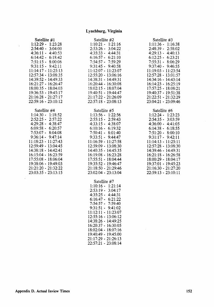
Satellite # 1 1:12:29 - 1:23:28 2:54:40 - 3:04:00 4:36: 11 - 4:40:53 6:14:42 - 6:18:42 7:51:15 - 8:00:06 9:31:15 - 9:42:11

11:14:17 - 11:25:13 12:57:34 - 13:08:35 14:39:52 - 14:49:33 16:21:27 - 16:26:47 18:00:35 - 18:04:03 19:36:53 - 19:45: 17 21:16:28 - 21:27:17 22:59:16 - 23:10:12

Satellite #4 1:14:30 - 1:18:52 2:52:25 - 2:57:22 4:29:28 - 4:38:47 6:09:58 - 6:20:57 7:53:07 - 8:04:08 9:36:14 - 9:47:14

11:18:23 - 11:27:43 12:59:49 - 13:04:45 14:38: 18 - 14:42:41 16:15:04 - 16:23:59 17:55:08 - 18:06:04 19:38:06 - 19:49:03 21:21:20 - 21:32:22 23:03:35 - 23: 13: 15


Lynchburg, Virginia

Satellite #2 1:10:21 - 1:21:16 2:53:26 - 3:04:22 4:35:33 - 4:44:31 6:16:57 - 6:21:10 7:54:57 - 7:59:29 9:31 :45 - 9:40:58

11:12:07- 11:23:07 12:55:20 - 13:06:16 14:38:31 - 14:49:31 16:20:44 - 16:30:08 18:02: 15 - 18:07:04 19:40:51 - 19:44:47 21:17:22 - 21:26:09 22:57:18 - 23:08:13

Satellite #5 1:13:56 - 1:22:56 2:55: 15 - 2:59:43 4:33: 15 - 4:38:07 6:10:16 - 6:19:32 7:50:41 - 8:01:40 9:33:51 - 9:44:47

11:16:59 - 11:27:58 12:59:09 - 13:08:30 14:40:35 - 14:45:35 16:19:08 - 16:23:28 17:55:51 - 18:04:44 19:35:52 - 19:46:47 21:18:50 - 21:29:46 23:02:04 - 23: 13:04

Satellite #7 1:10:16 - 1:21:14 2:53:19 - 3:04:17 4:35:25 - 4:44:31 6:16:47- 6:21:22 7:54:57 - 7:59:40 9:31:51 - 9:41:02

11:12:11 - 11:23:07 12:55:16 - 13:06:12 14:38:26 - 14:49:25 16:20:37 - 16:30:05 18:02:04 - 18:07:16 19:40:49 - 19:45:00 21:17:29 - 21:26:13 22:57:21 - 23:08: 14

Satellite #3 1:11:36- 1:16:38 2:48:39 - 2:58:02 4:29: 13 - 4:40: 13 6:12:25 - 6:23:21 7:55:31 - 8:06:29 9:37:40 - 9:46:55

11:19:03 - 11:23:54 12:57:28 - 13:01:57 14:34:16 - 14:43:14 16:14:23 - 16:25:19 17:57:25 - 18:08:21 19:40:37 - 19:51:38 21:22:51 - 21:32:29 23:04:21 - 23:09:46

Satellite #6 1:12:24 - 1:23:23 2:54:35 - 3:03:59 4:36:00 - 4:41:05 6:14:38 - 6:18:55 7:51:20 - 8:00:10 9:31:17 - 9:42:11

11: 14: 13 - 11:25:11 12:57:28 - 13:08:30 14:39:46 - 14:49:31 16:21:18 - 16:26:58 18:00:29 - 18:04: 17 19:37:01 - 19:45:23 21:16:30 - 21:27:20 22:59:13- 23:10:11

152

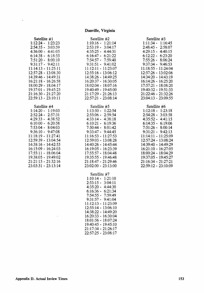
Satellite # l 1:12:24 - 1:23:23 2:54:35 - 3:03:59 4:36:00 - 4:41 :05 6:14:38 - 6:18:55 7:51:20 - 8:00:10 9:31:17 - 9:42:11

11:14:13 - 11:25:11 12:57:28 - 13:08:30 14:39:46 - 14:49:31 16:21:18 - 16:26:58 18:00:29 - 18:04: 17 19:37:01 - 19:45:23 21:16:30 - 21:27:20 22:59:13- 23:10:11

Satellite #4 1:14:20 - 1:19:03 2:52:24 - 2:57:31 4:29:33 - 4:38:52 6:10:00 - 6:20:58 7:53:04 - 8:04:03 9:36: 10 - 9:47:08

11:18:19 - 11:27:41 12:59:39 - 13:04:54 14:38: 16 - 14:42:53 16:15:09 - 16:24:03 17:55: 11 - 18:06:04 19:38:05 - 19:49:02 21:21:15 - 21:32:16 23:03:31 - 23: 13: 14


Danville, Virginia

Satellite #2 1:10:16 - 1:21:14 2:53: 19 - 3:04: 17 4:35:25 - 4:44:31 6:16:47 - 6:21:22 7:54:57 - 7:59:40 9:31:51 - 9:41:02

11:12:11 - 11:23:07 12:55:16 - 13:06:12 14:38:26 - 14:49:25 16:20:37 - 16:30:05 18:02:04 - 18:07: 16 19:40:49 - 19:45:00 21:17:29 - 21:26:13 22:57:21 - 23:08:14

Satellite #5 1:13:50 - 1:22:54 2:55:06 - 2:59:54 4:33: 14 - 4:38: 18 6:10:21 - 6:19:36 7:50:44 - 8:01:42 9:33:47 - 9:44:45

11:16:53 - 11:27:53 12:59:03 - 13:08:28 14:40:26 - 14:45:44 16:19:05 - 16:23:39 17:55:57 - 18:04:48 19:35:55 - 19:46:48 21:18:47 - 21:29:46 23:02:00 - 23: 13:00

Satellite #7 1:10:14 - 1:21:10 2:53:15- 3:04:11 4:35:20 - 4:44:30 6:16:36 - 6:21:34 7:54:55 - 7:59:49 9:31:57 - 9:41:04

11:12:13 - 11:23:09 12:55:14 - 13:06:10 14:38:22 - 14:49:20 16:20:33 - 16:30:04 18:01:56 - 18:07:24 19:40:45 - 19:45: l 0 21:17:34 - 21:26:17 22:57:25 - 23:08: 17

Satellite #3 1:11:34 - 1:16:45 2:48:45 - 2:58:07 4:29:15 - 4:40:15 6: 12:22 - 6:23:20 7:55:26 - 8:06:24 9:37:34 - 9:46:53

11:18:55 - 11:24:04 12:57:26 - 13:02:06 14:34:20 - 14:43:19 16:14:26 - 16:25:20 17:57:21 - 18:08:20 19:40:32 - 19:51 :33 21:22:46 - 21:32:26 23:04: 13 - 23:09:55

Satellite #6 1:12:18 - 1:23:18 2:54:28 - 3:03:58 4:35:52 - 4:41:15 6:14:35 - 6:19:06 7:51:26- 8:00:14 9:31:21 - 9:42:13

11:14:11 - 11:25:09 12:57:24 - 13:08:24 14:39:40 - 14:49:29 16:21:10 - 16:27:05 18:00:24 - 18:04:29 19:37:05 - 19:45:27 21:16:34 - 21:27:21 22:59:12 - 23:10:09

153

Satellite # 1 1:12:18 - 1:23:18 2:54:28 - 3:03:58 4:35:52 - 4:41:15 6:14:35 - 6:19:06 7:51:26 - 8:00:14 9:31:21 - 9:42: 13

11: 14:11 - 11:25:09 12:57:24 - 13:08:24 14:39:40 - 14:49:29 16:21:10 - 16:27:05 18:00:24 - 18:04:29 19:37:05 - 19:45:27 21:16:34 - 21:27:21 22:59:12 - 23:10:09

Satellite #4 1:14:00 - 1:19:13 2:52: 12 - 2:57:50 4:29:40 - 4:39:02 6:10:09 - 6:21:06 7:53:05 - 8:04:06 9:36:05 - 9:47:01

11:18:09 - 11:27:32 12:59:22 - 13:05:00 14:37:59 - 14:43:12 16:15:13 - 16:24:14 17:55:19 - 18:06:14 19:38:06 - 19:49:06 21:21: 11 - 21:32: 11 23:03:21 - 23: 13:03


Roanoke, Virginia

Satellite #2 1:10:14 - 1:21:10 2:53: 15 - 3:04: 11 4:35:20 - 4:44:30 6:16:36 - 6:21:34 7:54:55 - 7:59:49 9:31:57 - 9:41:04

11:12:13 - 11:23:09 12:55:14 - 13:06:10 14:38:22 - 14:49:20 16:20:33 - 16:30:04 18:01:56 - 18:07:24 19:40:45 - 19:45: 10 21:17:34 - 21:26:17 22:57:25 - 23:08:17

Satellite #5 1:13:40 - 1:22:46 2:54:46 - 3:00:03 4:33:00 - 4:38:36 6: 10:26 - 6: 19:47 7:50:54 - 8:01:51 9:33:49 - 9:44:49

11:16:49 - 11:27:47 12:58:54 - 13:08:20 14:40:07 - 14:45:50 16:18:47 - 16:23:58 17:56:01 - 18:04:59 19:36:04 - 19:46:57 21:18:50 - 21:29:50 23:01:55 - 23:12:55

Satellite #7 1:10:14 - 1:21:14 2:53:09 - 3:04:04 4:35: 11 - 4:44:22 6:16:17 - 6:21:41 7:54:41 - 8:00:08 9:32:02 - 9:41: 15

11:12:22 - 11:23:18 12:55: 14 - 13:06: 14 14:38:16 - 14:49:14 16:20:22 - 16:29:54 18:01:38 - 18:07:28 19:40:27 - 19:45:31 21:17:38 - 21:26:29 22:57:33 - 23:08:25

Satellite #3 1:11:22 - 1:17:04 2:48:51 - 2:58:17 4:29:25 - 4:40:23 6:12:23 - 6:23:22 7:55:21 - 8:06:18 9:37:25 - 9:46:45

11:18:36 - 11:24:10 12:57:09 - 13:02:25 14:34:25 - 14:43:31 16: 14:35 - 16:25:30 17:57:24 - 18:08:24 19:40:27 - 19:51:27 21:22:36 - 21:32:16 23:03:55 - 23:09:57

Satellite #6 1:12:13 - 1:23:12 2:54:19 - 3:03:48 4:35:34 - 4:41:20 6:14:18 - 6:19:24 7:51:31 - 8:00:25 9:31 :30 - 9:42:22

11:14:13 - 11:25:14 12:57:20 - 13:08:20 14:39:31 - 14:49: 18 16:20:53 - 16:27:06 18:00:04 - 18:04:51 19:37:08 - 19:45:40 21:16:44 - 21:27:30 22:59:16 - 23:10:15

154

Satellite # 1 1:12:13 - 1:23:12 2:54: 19 - 3:03:48 4:35:34 - 4:41 :20 6:14:18 - 6:19:24 7:51 :31 - 8:00:25 9:31 :30 - 9:42:22

11:14:13 - 11:25:14 12:57:20 - 13:08:20 14:39:31 - 14:49:18 16:20:53 - 16:27:06 18:00:04 - 18:04:51 19:37:08 - 19:45:40 21:16:44 - 21:27:30 22:59:16 - 23:10:15

Satellite #4 1:13:00 - 1:19:48 2:51:47 - 2:58:46 4:30:09 - 4:39:39 6: 10:39 - 6:21 :30 7:53:03 - 8:04:05 9:35:40 - 9:46:32

11:17:31 - 11:27:05 12:58:25 - 13:05:28 14:37:27 - 14:44:11 16: 15:40 - 16:24: 53 17:55:51 - 18:06:38 19:38:09 - 19:49:09 21:20:48 - 21:31:43 23:02:45 - 23: 12:33


Abingdon, Virginia

Satellite #2 1:10:14- 1:21:14 2:53:09 - 3:04:04 4:35: 11 - 4:44:22 6:16:17 - 6:21:41 7:54:41 - 8:00:08 9:32:02 - 9:41: 15

11:12:22- 11:23:18 12:55:14 - 13:06:14 14:38:16 - 14:49:14 16:20:22 - 16:29:54 18:01:38 - 18:07:28 19:40:27 - 19:45:31 21:17:38 - 21:26:29 22:57:33 - 23:08:25

Satellite #5 1:13:01 - 1:22:22 2:53:47 - 3:00:36 4:32:35 - 4:39:34 6: l 0: 56 - 6:20:23 7:51:22 - 8:02:14 9:33:47 - 9:44:49

11:16:24- 11:27:15 12:58:16 - 13:07:51 14:39:12 - 14:46:15 16:18:15 - 16:24:57 17:56:27 - 18:05:38 19:36:37 - 19:47:23 21: 18:51 - 21:29:54 23:01:32 - 23:12:28

Satellite #7 1:10:10 - 1:21:10 2:52:44 - 3:03:32 4:34:32 - 4:43:55 6:15:19 - 6:22:14 7:54:13 - 8:01:05 9:32:31 - 9:41:54

11:12:53 - 11:23:41 12:55:14 - 13:06:16 14:37:51 - 14:48:45 16: 19:47 - 16:29:26 18:00:43 - 18:07:53 19:39: 50 - 19:46:32 21:18:01 - 21:27:09 22:58:07 - 23:08:51

Satellite #3 1:11:00 - 1:18:01 2:49:21 - 2:58:53 4:29:53 - 4:40:45 6:12:20 - 6:23:21 7:54:56 - 8:05:46 9:36:47 - 9:46:17

11:17:39 - 11:24:38 12:56:38 - 13:03:24 14:34:52 - 14:44:09 16:15:06 - 16:25:54 17:57:25 - 18:08:26 19:40:04 - 19:50:59 21:22:01 - 21:31:47 23:03:0 l - 23: 10: 18

Satellite #6 1:11:48 - 1:22:42 2:53:43 - 3:03: 19 4:34:38 - 4:41 :45 6:13:44 - 6:20:25 7:51:56 - 8:01:05 9:32:02 - 9:42:47

11:14:17 - 11:25:18 12:56:57 - 13:07:53 14:38:56 - 14:48:47 16:20:00 - 16:27:24 17:59:20-18:05:52 19:37:28 - 19:46:21 21:17:19 - 21:27:58 22: 59:22 - 23: 10:23

155

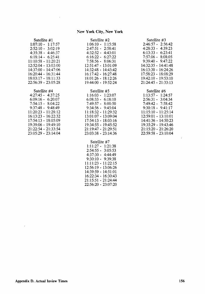
Satellite # l 1:07:10 - 1:17:57 2: 52: 10 - 3:02: 19 4:35:38 - 4:46:37 6:18:14 - 6:25:41

11:10:58 - 11:20:21 12:52:04 - 13:03:00 14:37:00 - 14:47:06 16:20:44 - 16:31 :44 18:03: 17 - 18: 11 :33 22:56:39 - 23:05:28

Satellite #4 4:27:45 - 4:37:25 6:09: 16 - 6:20:07 7:54:15 - 8:04:22 9:37:48 - 9:48:49

11:20:23 - 11:28:12 16: 13:23 - 16:22:32 17:54:13 - 18:05:09 19:39:06 - 19:49: 10 21:22:54 - 21:33:54 23:05:29 - 23: 14:04


New York City, New York

Satellite #2 1:06:10 - 1:15:58 2:47:51 - 2:58:41 4:32:52 - 4:43:01 6: 16:22 - 6:27:22 7:58:56 - 8:06:31

12:51:47 - 13:01:09 14:32:48 - 14:43:42 16:17:42 - 16:27:48 18:01:26 - 18:12:26 19:44:00 - 19: 52:24

Satellite #5 1: 16:03 - 1 :23:07 6:08:33 - 6:18:10 7:49:57 - 8:00:50 9:34:56 - 9:45:04

11: 18:32 - 11 :29:32 13:01:07 - 13:09:04 17:54:13 - 18:03:16 19:34:55 - 19:45:52 21:19:47 - 21:29:51 23:03:38 - 23: 14:36

Satellite #7 1:11:27 - 1:21:38 2:54:55 - 3:05:53 4:37:30 - 4:44:49 9:30: 10 - 9:39:38

11:11:23 - 11:22:15 12:56:19 - 13:06:26 14:39:59 - 14:51:01 16:22:34 - 16:30:43 21:15:51 - 21:24:44 22:56:20 - 23:07:20

Satellite #3 2:46:57 - 2:56:42 4:28:33 - 4:39:23 6: 13:33 - 6:23:41 7:57:06 - 8:08:05 9:39:40 - 9:47:22

14:32:35 - 14:41:48 16: 13:30 - 16:24:26 17:58:23 - 18:08:29 19:42:10 - 19:53:10 21:24:45 - 21:33:13

Satellite #6 1:13:57 - 1:24:57 2:56:31 - 3:04:34 7:49:42 - 7:58:42 9:30:18 - 9:41:17

11:15:10 - 11:25:14 12:59:01 - 13:10:01 14:41:36 - 14:50:23 19:35:29 - 19:43:46 21:15:20 - 21:26:20 22:59:58 - 23: 10:04

156

Satellite # 1 1:13:57 - 1:24:57 2:56:31 - 3:04:34 7:49:42 - 7:58:42 9:30: 18 - 9:41: 17

11:15:10 - 11:25:14 12:59:01 - 13:10:01 14:41:36 - 14:50:23 19:35:29 - 19:43:46 21:15:20 - 21:26:20 22:59:58 - 23: 10:04

Satellite #4 4:28:24 - 4:37:39 6:09:10 - 6:20:10 7:53:36 - 8:03:59 9:37:15 - 9:48:15

11: 19:43 - 11 :28:27 16:14:05 - 16:22:46 17:54:13 - 18:05:14 19:38:28 - 19:48:51 21:22:19 - 21:33:19 23:04:51 - 23:14:08


Philadelphia, Pennsylvania

Satellite #2 1:11:27 - 1:21:38 2:54:55 - 3:05:53 4:37:30 - 4:44:49 9:30:10 - 9:39:38

11: 11 :23 - 11:22:15 12:56:19 - 13:06:26 14:39:59 - 14:51:01 16:22:34 - 16:30:43 21:15:51 - 21:24:44 22:56:20 - 23:07:20

Satellite #5 1:15:19 - 1:23:30 6:09: 13 - 6: 18:22 7:49:54 - 8:00:52 9:34: 18 - 9:44:41

11:17:58 - 11:28:59 13:00:27 - 13:09:17 17:54:55-18:03:30 19:34:56 - 19:45:58 21:19:09 - 21:29:34 23:03:02 - 23: 14:0 l

Satellite #7 1:10:48 - 1:21:14 2:54:20 - 3:05:22 4:36:47 - 4:45: l 0 9:30:50 - 9:39:50

11:11:19 - 11:22:19 12:55:41 - 13:06:05 14:39:25 - 14:50:25 16:21:56 - 16:30:55 21:16:33 - 21:24:57 22:56:24 - 23:07:24

Satellite #3 2:47:36 - 2:56:54 4:28:27 - 4:39:26 6:12:54 - 6:23:19 7:56:31 - 8:07:32 9:39:00 - 9:47:37

14:33: 17 - 14:42:0 l 16: 13:30 - 16:24:30 17:57:45 - 18:08: 10 19:41:35 - 19:52:35 21:24:07 - 21:33:20

Satellite #6 1: 13:24 - l :24:24 2:55:52 - 3:04:45 7:50:24 - 7:58:54 9:30:21 - 9:41:21

11:14:32 - 11:24:57 12:58:27 - 13:09:25 14:41:00 - 14:50:25 19:36: 14 - 19:44:0 l 21:15:28 - 21:26:28 22:59:23 - 23:09:49

157

Satellite # 1 1: 13:24 - 1 :24:24 2:55:52 - 3:04:45 7:50:24 - 7:58:54 9:30:21 - 9:41:21

11:14:32 - 11:24:57 12:58:27 - 13:09:25 14:41:00 - 14:50:25 19:36: 14 - 19:44:0 l 21:15:28 - 21:26:28 22:59:23 - 23:09:49

Satellite #4 2:53:38 - 2:55:23 4:28:50 - 4:38:06 6:09:28 - 6:20:30 7:53:21 - 8:04:03 9:36:50 - 9:47:50

11:19:10 - 11:28:10 16:14:30 - 16:23:16 17:54:34 - 18:05:34 19:38:17 - 19:48:58 21:21:53 - 21:32:54 23:04:20 - 23: 13:48


Washington, D. C.

Satellite #2 1:10:48 - 1:21:14 2:54:20 - 3:05:22 4:36:47 - 4:45:10 9:30:50 - 9:39:50

11: 11: 19 - 11:22:19 12:55:41 - 13:06:05 14:39:25 - 14:50:25 16:21:56 - 16:30:55 21:16:33 - 21:24:57 22:56:24 - 23:07:24

Satellite #5 1:14:45 - 1:23:18 4:34:37 - 4:36:01 6:09:39 - 6: 18:51 7:50:12 - 8:01:13 9:34:03 - 9:44:45

11:17:33 - 11:28:33 12:59:55 - 13:08:58 14:43: 14 - 14:43:21 17:55:19 - 18:03:59 19:35:18 - 19:46:18 21:18:58 - 21:29:39 23:02:38 - 23: 13:38

Satellite #7 1:10:32 - 1:21:15 2:53:56 - 3:04:54 4:36:14 - 4:44:55 9:31:15 - 9:40:18

11:11:40 - 11:22:40 12:55:28 - 13:06:08 14:39:00 - 14:50:02 16:21:23 - 16:30:36 18:04:10 - 18:05:40 21:16:56 - 21:25:28 22:56:47 - 23:07:46

Satellite #3 1:12:40 - 1:14:43 2:48:02 - 2:57:21 4:28:45 - 4:39:45 6:12:40 - 6:23:21 7:56:05 - 8:07:06 9:38:26 - 9:47:22

14:33:42 - 14:42:32 16:13:50 - 16:24:50 17:57:34 - 18:08:16 19:41:10 - 19:52:12 21:23:36 - 21:33:00 23:06:08 - 23:08:30

Satellite #6 1:12:58 - 1:23:59 2:55: 19 - 3:04:28 4:38: 18 - 4:39: 17 7:50:49 - 7:59:26 9:30:44 - 9:41 :42

11: 14:22 - 11 :25:03 12:58:02 - 13:09:02 14:40:28 - 14:50:04 16:22:54 - 16:25:57 19:36:34 - 19:44:35 21:15:54 - 21:26:48 22:59:16 - 23:10:00

158

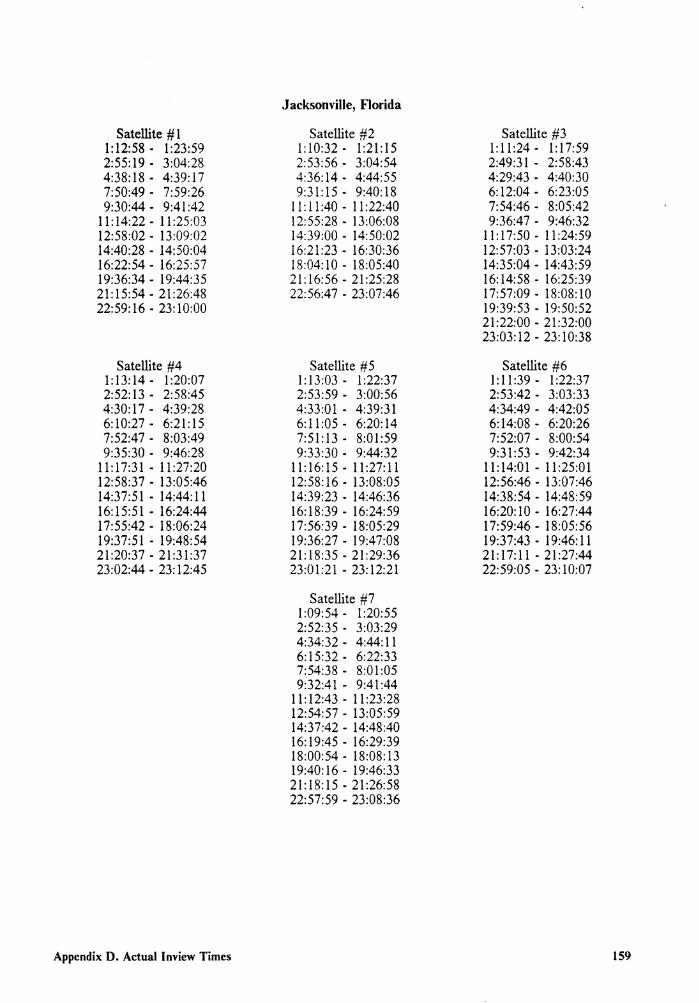
Satellite # 1 1: 12:58 - 1 :23:59 2:55: 19 - 3:04:28 4:38: 18 - 4:39: 17 7:50:49 - 7:59:26 9:30:44 - 9:41:42

11:14:22 - 11:25:03 12:58:02 - 13:09:02 14:40:28 - 14:50:04 16:22:54 - 16:25:57 19:36:34 - 19:44:35 21:15:54 - 21:26:48 22:59:16 - 23:10:00

Satellite #4 1:13:14 - 1:20:07 2:52:13 - 2:58:45 4:30: 17 - 4:39:28 6:10:27 - 6:21:15 7:52:47 - 8:03:49 9:35:30 - 9:46:28

11:17:31 - 11:27:20 12:58:37 - 13:05:46 14:37:51- 14:44:11 16:15:51 - 16:24:44 17:55:42 - 18:06:24 19:37:51 - 19:48:54 21:20:37 - 21:31:37 23:02:44 - 23: 12:45


Jacksonville, Florida

Satellite #2 1:10:32 - 1:21:15 2:53:56 - 3:04:54 4:36:14 - 4:44:55 9:31:15 - 9:40:18

11:11:40 - 11:22:40 12:55:28 - 13:06:08 14:39:00 - 14:50:02 16:21 :23 - 16:30:36 18:04:10 - 18:05:40 21:16:56 - 21:25:28 22:56:47 - 23:07:46

Satellite #5 1:13:03 - 1:22:37 2:53:59 - 3:00:56 4:33:0 l - 4:39:31 6:11:05- 6:20:14 7:51:13 - 8:01:59 9:33:30 - 9:44:32

11:16:15 - 11:27:11 12:58:16 - 13:08:05 14:39:23 - 14:46:36 16: 18:39 - 16:24:59 17:56:39 - 18:05:29 19:36:27 - 19:47:08 21: 18:35 - 21:29:36 23:01:21 - 23:12:21

Satellite #7 1:09:54 - 1:20:55 2:52:35 - 3:03:29 4:34:32 - 4:44: 11 6: 15:32 - 6:22:33 7:54:38 - 8:01 :05 9:32:41 - 9:41 :44

11:12:43 - 11:23:28 12:54:57 - 13:05:59 14:37:42 - 14:48:40 16: 19:45 - 16:29:39 18:00:54 - 18:08:13 19:40: 16 - 19:46:33 21:18:15 - 21:26:58 22:57:59 - 23:08:36

Satellite #3 1:11:24 - 1:17:59 2:49:31 - 2:58:43 4:29:43 - 4:40:30 6:12:04 - 6:23:05 7:54:46 - 8:05:42 9:36:47 - 9:46:32

11:17:50 - 11:24:59 12:57:03 - 13:03:24 14:35:04 - 14:43:59 16: 14: 58 - 16:25:39 17:57:09 - 18:08:10 19:39:53 - 19:50:52 21:22:00 - 21:32:00 23:03: 12 - 23: 10:38

Satellite #6 1:11:39 - 1:22:37 2:53:42 - 3:03:33 4:34:49 - 4:42:05 6: 14:08 - 6:20:26 7:52:07 - 8:00:54 9:31:53 - 9:42:34

11:14:01 - 11:25:01 12:56:46 - 13:07:46 14:38:54 - 14:48:59 16:20:10 - 16:27:44 17:59:46 - 18:05:56 19:37:43 - 19:46:11 21:17:11 - 21:27:44 22:59:05 - 23: 10:07

159

Satellite # 1 1:11:39 - 1:22:37 2:53:42 - 3:03:33 4:34:49 - 4:42:05 6: 14:08 - 6:20:26 7:52:07 - 8:00:54 9:31:53 - 9:42:34

11:14:01 - 11:25:01 12:56:46 - 13:07:46 14:38:54 - 14:48:59 16:20:10 - 16:27:44 17:59:46 - 18:05:56 19:37:43 - 19:46: 11 21:17:11 - 21:27:44 22:59:05 - 23: 10:07

Satellite #4 1:12:29 - 1:19:45 2:51:23 - 2:59:08 4:30:15 - 4:40:03 6:11:01 - 6:21:52 7:53:17 - 8:04:16 9:35:36 - 9:46: 19

11:17:16 - 11:26:40 12:57:55 - 13:05:21 14:36:58 - 14:44:32 16:15:43 - 16:25:18 17:56:13 - 18:07:01 19:38:22 - 19:49:22 21:20:45 - 21:31:33 23:02:30 - 23:12:09


Detroit, Michigan

Satellite #2 1:09:54 - 1:20:55 2:52:35 - 3:03:29 4:34:32 - 4:44: 11 6: 15:32 - 6:22:33 7:54:38 - 8:01:05 9:32:41 - 9:41:44

11:12:43 - 11:23:28 12:54:57 - 13:05:59 14:37:42 - 14:48:40 16: 19:45 - 16:29:39 18:00:54 - 18:08:"13 19:40:16 - 19:46:33 21:18:15 - 21:26:58 22:57:59 - 23:08:36

Satellite #5 1:12:44 - 1:21:56 2:53: 15 - 3:00:34 4:32:11 - 4:39:55 6:11:03 - 6:20:48 7:51:45 - 8:02:35 9:33:59 - 9:45:00

11:16:21- 11:27:05 12:58:00 - 13:07:27 14:38:41 - 14:46:09 16:17:45 - 16:25:19 17:56:31 - 18:06:03 19:36:58 - 19:47:45 21:19:06 - 21:30:06 23:01:29 - 23:12:18

Satellite #7 1:10:21 - 1:21:20 2:52:38 - 3:03: 19 4:34:15 - 4:43:31 6: 14:49 - 6:22: 10 7:53:46 - 8:01:28 9:32:37 - 9:42:18

11:13:14 - 11:24:04 12:55:28 - 13:06:28 14:37:48 - 14:48:34 16: 19:31 - 16:29:00 18:00:13 - 18:07:44 19:39:22 - 19:46:52 21:18:04 - 21:27:33 22:58:29 - 23:09: 14

Satellite #3 1:10:35 - 1:18:22 2:49:30 - 2:59: 17 4:30:16 - 4:41:07 6: 12:32 - 6:23:33 7:54:51 - 8:05:34 9:36:31 - 9:45:52

11: 17:08 - 11:24:32 12:56: 10 - 13:03:45 14:34:56 - 14:44:32 16:15:28 - 16:26:16 17:57:40 - 18:08:39 19:40:01 - 19:50:49 21:21:46 - 21:31:21 23:02:33 - 23: 10:08

Satellite #6 1:11:46 - 1:22:31 2:53:26 - 3:02:55 4:34:08 - 4:41:38 6: 13: 14 - 6:20:45 7:51:59 - 8:01:28 9:32:25 - 9:43: 10

11:14:32- 11:25:32 12:56:55 - 13:07:44 14:38:41 - 14:48:23 16:19:32 - 16:27:13 17:58:49- 18:06:11 19:37:28 - 19:46:44 21:17:39 - 21:28:21 22:59:39 - 23: 10:38

160

Satellite # l 1:11:46 - 1:22:31 2:53:26 - 3:02:55 4:34:08 - 4:41 :38 6:13:14 - 6:20:45 7:51:59 - 8:01:28 9:32:25 - 9:43: 10

11:14:32 - 11:25:32 12:56:55 - 13:07:44 14:38:41 - 14:48:23 16:19:32 - 16:27:13 17:58:49 - 18:06: 11 19:37:28 - 19:46:44 21:17:39 - 21:28:21 22:59:39 - 23:10:38

Satellite #4 1:11:31 - 1:20:19 2:51:19 - 3:00:14 4:31:06 - 4:40:56 6:11:45 - 6:22:18 7:53:17 - 8:04:01 9:34:58 - 9:45:27

11:16:17 - 11:26:02 12:56:54 - 13:05:46 14:36:45 - 14:45:37 16:16:29 - 16:26:13 17:57:02 - 18:07:31 19:38:29 - 19:49:13 21:20:11 - 21:30:44 23:01:34 - 23:11:25


Indianapolis, Indiana

Satellite #2 1:10:21 - 1:21:20 2:52:38 - 3:03: 19 4:34: 15 - 4:43:31 6: 14:49 - 6:22: 10 7:53:46 - 8:01:28 9:32:37 - 9:42:18

11:13:14- 11:24:04 12:55:28 - 13:06:28 14:37:48 - 14:48:34 16:19:31 - 16:29:00 18:00:13 - 18:07:44 19:39:22 - 19:46:52 21:18:04 - 21:27:33 22:58:29 - 23:09: 14

Satellite #5 1:11:44- 1:21:24 2:52:17 - 3:01:06 4:32:05 - 4:41:00 6:11:51- 6:21:40 7:52:30 - 8:03:02 9:34:01 - 9:44:45

11:15:44- 11:26:14 12:57:03 - 13:06:47 14:37:40 - 14:46:32 16: 17:33 - 16:26:23 17:57:15 - 18:06:58 19:37:47 - 19:48:16 21:19:13 - 21:29:58 23:00:56 - 23: 11 :29

Satellite #7 1:10:18 - 1:21:01 2:52:00 - 3:02:27 4:33:15 - 4:42:57 6:13:49 - 6:22:40 7:53:39 - 8:02:31 9:33:24 - 9:43: 12

11:14:01- 11:24:31 12:55:30 - 13:06: 14 14:37:13 - 14:47:44 16:18:34 - 16:28:21 17:59: 12 - 18:08:06 19:39:06 - 19:47:54 21:18:49 - 21:28:29 22:59: 17 - 23:09:45

Satellite #3 1:10:31 - 1:19:28 2:50:20 - 3:00: 11 4:31:00 - 4:41:32 6:12:31 - 6:23:16 7:54:14 - 8:04:43 9:35:32 - 9:45:16

11:16:09 - 11:24:59 12:55:58 - 13:04:50 14:35:44 - 14:45:27 16:16:17 - 16:26:47 17:57:44 - 18:08:28 19:39:26 - 19:49:59 21:20:48 - 21:30:39 23:01:30 - 23:10:27

Satellite #6 1:11:08 - 1:21:40 2:52:29 - 3:02:15 4:33:08 - 4:42:01 6:13:00 - 6:21:50 7:52:42 - 8:02:25 9:33: 13 - 9:43:42

11:14:38- 11:25:22 12:56:21 - 13:06:56 14:37:46 - 14:47:39 16:18:30 - 16:27:28 17:58:26 - 18:07:13 19:38:07 - 19:47:42 21:18:31 - 21:28:56 22:59:51 - 23:10:34

161

Satellite # 1 1:11:08 - 1:21:40 2:52:29 - 3:02:15 4:33:08 - 4:42:01 6:13:00 - 6:21:50 7:52:42 - 8:02:25 9:33: 13 - 9:43:42

11:14:38 - 11:25:22 12:56:21 - 13:06:56 14:37:46 - 14:47:39 16:18:30 - 16:27:28 17:58:26 - 18:07:13 19:38:07 - 19:47:42 21:18:31 - 21:28:56 22:59:51 - 23:10:34

Satellite #4 1:11:05 - 1:20:24 2:51:15 - 3:00:41 4:31:29 - 4:41:24 6: 12: 11 - 6:22:33 7:53:23 - 8:03:53 9:34:45 - 9:45:02

11:15:50- 11:25:39 12:56:27 - 13:05:49 14:36:39 - 14:46:01 16: 16:49 - 16:26:42 17:57:29 - 18:07:47 19:38:39 - 19:49:09 21:19:59 - 21:30:20 23:01:07 - 23:11:01


Chicago, Illinois

Satellite #2 1:10:18 - 1:21:01 2:52:00 - 3:02:27 4:33: 15 - 4:42:57 6: 13:49 - 6:22:40 7:53:39 - 8:02:31 9:33:24 - 9:43: 12

11: 14:01 - 11:24:31 12:55:30 - 13:06:14 14:37:13 - 14:47:44 16:18:34 - 16:28:21 17:59: 12 - 18:08:06 19:39:06 - 19:47:54 21:18:49 - 21:28:29 22:59: 17 - 23:09:45

Satellite #5 1:11:17 - 1:21:03 2:51:51 - 3:01:12 4:32:01 - 4:41:26 6: 12: 13 - 6:22:08 7:52:57 - 8:03: 17 9:34:08 - 9:44:38

11:15:29 - 11:25:47 12:56:35 - 13:06:24 14:37:13 - 14:46:34 16:17:26 - 16:26:47 17:57:36 - 18:07:27 19:38:13 - 19:48:34 21:19:24 - 21:29:54 23:00:44 - 23: 11 :05

Satellite #7 1:10:24 - 1:20:54 2:51:43 - 3:02:00 4:32:48 - 4:42:34 6: 13:23 - 6:22:43 7:53:34 - 8:02:58 9:33:45 - 9:43:40

11:14:28 - 11:24:48 12:55:39 - 13:06:08 14:37:00 - 14:47:18 16:18:05 - 16:27:56 17:58:45 - 18:08:07 19:38:58 - 19:48:20 21:19:08 - 21:28:57 22:59:45 - 23: 10:04

Satellite #3 1:10:29 - 1:19:54 2:50:42 - 3:00:38 4:31:26 - 4:41:47 6:12:39 - 6:23:08 7:54:00 - 8:04:16 9:35:04 - 9:44:53

11:15:40 - 11:25:03 12:55:53 - 13:05: 15 14:36:03 - 14:45:56 16:16:44 - 16:27:02 17:57:53 - 18:08:24 19:39:14 - 19:49:35 21:20:22 - 21:30:14 23:01:02 - 23:10:27

Satellite #6 1:10:56 - 1:21:14 2:52:02 - 3:01:51 4:32:39 - 4:42:02 6:12:52 - 6:22:15 7:53:02 - 8:02:54 9:33:40 - 9:43:59

11:14:49 - 11:25:20 12:56:10 - 13:06:31 14:37:19 - 14:47:14 16:18:01 - 16:27:25 17:58:15 - 18:07:36 19:38:25 - 19:48:12 21:18:58 - 21:29:15 23:00:05 - 23: 10:34

162

Satellite # 1 1:10:56 - 1:21:14 2:52:02 - 3:01:51 4:32:39 - 4:42:02 6:12:52 - 6:22:15 7:53:02 - 8:02:54 9:33:40 - 9:43:59

11:14:49 - 11:25:20 12:56:10 - 13:06:31 14:37:19 - 14:47:14 16:18:01 - 16:27:25 17:58:15 - 18:07:36 19:38:25 - 19:48: 12 21:18:58 - 21:29:15 23:00:05 - 23: 10:34

Satellite #4 1:10:33 - 1:20:33 2:51:19 - 3:01:18 4:32:05 - 4:42:05 6: 12:50 - 6:22:49 7:53:36 - 8:03:36 9:34:22 - 9:44:20

11:15:06- 11:25:07 12:55:53 - 13:05:51 14:36:37 - 14:46:38 16: 17:23 - 16:27:24 17:58:10 - 18:08:09 19:38:55 - 19:48:54 21:19:40 - 21:29:39 23:00:25 - 23: 10:26


Memphis, Tennessee

Satellite #2 1:10:24 - 1:20:54 2:51:43 - 3:02:00 4:32:48 - 4:42:34 6: 13:23 - 6:22:43 7:53:34 - 8:02:58 9:33:45 - 9:43:40

11:14:28 - 11:24:48 12:55:39 - 13:06:08 14:37:00 - 14:47:18 16:18:05 - 16:27:56 17:58:45 - 18:08:07 19:38:58 - 19:48:20 21:19:08 - 21:28:57 22: 59:45 - 23: 10:04

Satellite #5 1:10:33 - 1:20:33 2:51:19 - 3:01:18 4:32:05 - 4:42:05 6:12:50 - 6:22:51 7:53:37 - 8:03:36 9:34:22 - 9:44:24

11: 15:06 - 11 :25:07 12:55:53 - 13:05:51 14:36:37 - 14:46:38 16:17:23 - 16:27:24 17:58:10 - 18:08:10 19:38:55 - 19:48:54 21:19:40 - 21:29:39 23:00:25 - 23: 10:26

Satellite #7 1: 10:33 - 1 :20:33 2:51:19 - 3:01:18 4:32:05 - 4:42:04 6:12:49 - 6:22:49 7:53:36 - 8:03:36 9:34:22 - 9:44:22

11:15:08 - 11:25:07 12:55:53 - 13:05:51 14:36:37 - 14:46:38 16: 17:23 - 16:27:22 17:58:08 - 18:08:09 19:38:55 - 19:48:54 21:19:40 - 21:29:41 23:00:27 - 23: 10:26

Satellite #3 1:10:33 - 1:20:34 2:51:20 - 3:01:18 4:32:05 - 4:42:05 6: 12:50 - 6:22:49 7:53:36 - 8:03:34 9:34:20 - 9:44:20

11:15:06 - 11:25:07 12:55:53 - 13:05:53 14:36:39 - 14:46:38 16: 17:23 - 16:27:24 17:58: 10 - 18:08:09 19:38:55 - 19:48:54 21:19:40 - 21:29:39 23:00:25 - 23: 10:26

Satellite #6 1:10:33 - 1:20:33 2:51:19 - 3:01:18 4:32:05 - 4:42:05 6:12:50 - 6:22:49 7:53:36 - 8:03:36 9:34:22 - 9:44:22

11:15:08 - 11:25:07 12:55:53 - 13:05:51 14:36:37 - 14:46:38 16:17:23 - 16:27:24 17:58:10 - 18:08:09 19:38:55 - 19:48:54 21:19:40 - 21:29:41 23:00:27 - 23: 10:26

163

Satellite # 1 1: 10:33 - 1 :20:33 2:51:19 - 3:01:18 4:32:05 - 4:42:05 6: 12:50 - 6:22:49 7:53:36 - 8:03:36 9:34:22 - 9:44:22

11:15:08 - 11:25:07 12:55:53 - 13:05:51 14:36:37 - 14:46:38 16:17:23 - 16:27:24 17:58: 10 - 18:08:09 19:38:55 - 19:48:54 21:19:40 - 21:29:41 23:00:27 - 23: 10:26

Satellite #4 1:09:23 - 1:20:13 2:51:25 - 3:02:18 4:33: 19 - 4:43:43 6:14:34 - 6:23:40 7:54:47 - 8:02:46 9:33:59 - 9:42:39

11:13:33 - 11:23:37 12:54:34 - 13:05:23 14:36:35 - 14:47:29 16:18:32 - 16:29:00 17:59:53 - 18:09:08 19:40: 15 - 19:48: 16 21:19:31 - 21:28:00 22:58:57 - 23:08:52


Houston, Texas

Satellite #2 1:10:33 - 1:20:33 2:51:19 - 3:01:18 4:32:05 - 4:42:04 6: 12:49 - 6:22:49 7:53:36 - 8:03:36 9:34:22 - 9:44:22

11: 15:08 - 11 :25:07 12:55:53 - 13:05:51 14:36:37 - 14:46:38 16:17:23 - 16:27:22 17:58:08 - 18:08:09 19:38:55 - 19:48:54 21:19:40 - 21:29:41 23:00:27 - 23: 10:26

Satellite #5 1:08:58 - 1:19:08 2:50:07 - 3:00:56 4:32: 10 - 4:43:03 6:14:05 - 6:24:27 7:55:20 - 8:04:27 9:35:34 - 9:43:33

11:14:47 - 11:23:24 12:54:19-13:04:22 14:35: 19 - 14:46:07 16:17:19 - 16:28:12 17:59:16 - 18:09:46 19:40:38 - 19:49:55 21:21:00 - 21:29:04 23:00: 18 - 23:08:47

Satellite #7 1:11:41 - 1:19:38 2:50:51 - 2:59:35 4:30:30 - 4:40:39 6: 11:37 - 6:22:25 7:53:39 - 8:04:31 9:35:34 - 9:45:58

11:16:51 - 11:26:00 12:57:07 - 13:05:09 14:36:22 - 14:44:57 16:15:52 - 16:25:53 17:56:48 - 18:07:35 19:38:48 - 19:49:40 21:20:46 - 21:31:18 23:02:08 - 23: 11 :28

Satellite #3 1:10:41 - 1:21:33 2:52:35 - 3:02:57 4:33:49 - 4:42:52 6:14:01 - 6:21:59 7:53:13 - 8:01:53 9:32:48 - 9:42:53

11:13:50 - 11:24:38 12:55:51 - 13:06:43 14:37:48 - 14:48:15 16:19:06 - 16:28:22 17:59:27 - 18:07:30 19:38:44 - 19:47:15 21:18:11 - 21:28:07 22:59:03 - 23:09:49

Satellite #6 1:10:16 - 1:18:52 2:49:46 - 2:59:48 4:30:45 - 4:41 :32 6: 12:45 - 6:23:38 7:54:42 - 8:05: 13 9:36:05 - 9:45:23

11: 16:28 - 11 :24:31 12:55:47 - 13:04: 14 14:35: 11 - 14:45:04 16:15:59 - 16:26:43 17:57:53 - 18:08:48 19:39:55 - 19:50:29 21:21:22 - 21:30:51 23:01:53 - 23:10:03

164

Satellite # 1 1:10:16 - 1:18:52 2:49:46 - 2:59:48 4:30:45 - 4:41 :32 6: 12:45 - 6:23:38 7:54:42 - 8:05: 13 9:36:05 - 9:45:23

11:16:28 - 11:24:31 12:55:47 - 13:04:14 14:35: 11 - 14:45:04 16:15:59 - 16:26:43 17:57:53 - 18:08:48 19:39:55 - 19:50:29 21:21:22 - 21:30:51 23:01:53 - 23:10:03

Satellite #4 1:09:19 - 1:14:01 2:57:52 - 3:02:25 4:39:23 - 4:50: 16

11:07:00 - 11:17:31 12:53:01 - 12:59:26 14:43:40 - 14:45:35 16:24:30 - 16:35:28 22:52:36 - 23:02:33


Los Angeles, California

Satellite #2 1:11:41- 1:19:38 2:50:51 - 2:59:35 4:30:30 - 4:40:39 6: 11 :37 - 6:22:25 7:53:39 - 8:04:31 9:35:34 - 9:45:58

11:16:51 - 11:26:00 12:57:07 - 13:05:09 14:36:22 - 14:44:57 16:15:52 - 16:25:53 17:56:48 - 18:07:35 19:38:48 - 19:49:40 21:20:46 - 21:31:18 23:02:08 - 23: 11:28

Satellite #5 1 :02:22 - 1: 13: 10 2:49:50 - 2:54:48 4:38:40 - 4:42:54 6:20:08 - 6:31:00

12:47:48 - 12:58:14 14:33:34 - 14:40: 11 16:24:41 - 16:25:50 18:05: 14 - 18: 16: 11

Satellite #7 4:23:54 - 4:34:37 6:10:51 - 6:16:22 8:00: 16 - 8:03:53 9:41:35 - 9:52:30

16:09:23 - 16:19:40 17:54:41 - 18:01:43 21:26:42 - 21:37:38

Satellite #3 1:17:05 - 1:21:55 2:58:40 - 3:09:29 9:26:14 - 9:36:49

11: 12:28 - 11: 18:40 13:02:46- 13:05:11 14:43:46 - 14:54:44 21:11:47 - 21:21:49 22:56:24 - 23:03:59

Satellite #6 2:43:16 - 2:53:38 4:28:49 - 4:35:38 8:00:39 - 8: 11 :36

14:28:56 - 14:38:39 16:12:52 - 16:20:56 19:45:47 - 19:56:33 21:30:50 - 21:32:49

165

Appendix E. Earth Station Component Specifications

The information contained in this appendix was obtained directly from the manufacturer, unless

otherwise stated.

E.l Computer

The GRiDLite Plus Computer has the following features:

IO inch 640x200 blue backlit Liquid Crystal Display (LCD) screen

128 kilobytes of RAM

capacity for 8 Read-Only Memory (ROMs) (1 megabyte)

71-key keyboard

one 1.4 megabyte 3-1/2 inch floppy diskette drive

110/220 volt ac autosensing power supply

parallel printer port

RS-232 serial port (25 pin)

Appendix E. Earth Station Component Specifications 166

RGB color video port (CGA)

external floppy diskette drive port

full system indicator lights

rechargeable internal battery pack

The GRiDLite Plus Computer has a 80C86 16-bit dual-speed microprocessor that operates at either

8 or 4.77 MHz. The base retail price for this computer is $1950. Additional accessories include:

640 kilobytes of RAM instead of the 128 kilobytes ($300)

1/2 megabytes EMS RAM ($395)

1 megabyte EMS RAM ($495)

20 megabyte hard disk drive instead of the floppy diskette drive ($1175)

Hayes Smartmodem compatible 2400/ 1200/300 bps modem ($595)

8087 arithmetic coprocessor ($195)

MS-DOS 3.21 in one 128 kilobyte 32-pin ROM ($200)

MS-DOS 3.21, includes 3-1/2 inch diskette and documentation ($150)

The weight of this model is 9.7 pounds or 4.4 kilograms (with battery) and it has a footprint of 11

inches by 13 inches. The case is an impact-resistant case.

The GRiDCase 1520 and 1530 Computers have the following features:

10 inch 640x400 yellow backlit LCD screen

1 megabyte of RAM

capacity for 2 ROMs (512 kilobytes)

72-key keyboard

two 1.4 megabyte 3-1/2 inch floppy diskette drive







external keyboard/keypad port


The GRiDCase 1520 Computer has a 80C286 16-bit microprocessor that operates at 10 MHz.

The base retail price for this computer is $3495. The GRiDCase 1530 Computer has a 80386 32-bit

microprocessor that operates at 12.5 MHz. The base retail price for this computer is $4695.

Additional accessories include:

10 inch 640x400 plasma screen ($995)

10 inch 640x400 blue backlit LCD screen ($295)

2 megabytes of RAM ($595)

4 megabytes of RAM ($2395)

20 megabyte hard disk and 1.4 megabyte 3-1/2 inch floppy diskette drive ($1175)

40 megabyte hard disk (single drive system) ($1675)

Hayes Smartmodem compatible 2400/ 1200/300 bps modem ($595)

80287 arithmetic coprocessor (for model 1520 only) ($495)

80387 arithmetic coprocessor (for model 1530 only) ($895)

MS-DOS 3.21 in one ROM ($200)

MS-DOS 3.21, includes 3-1/2 inch diskette and documentation ($150)

The weight of these models range from 11.5 to 13.5 pounds or 5.1 to 6.0 kilograms, depending on

configuration. The dimensions are 2.3 inches (height) x 11.5 inches (width) x 15.0 inches (length).

The case is a rugged magnesium case.

The GRiDCase 1535 EXP Computer has the following features:


10 inch 640x400 blue backlit LCD screen

1 megabyte of RAM

capacity for 2 ROMs (512 kilobytes)

72-key keyboard

40 megabyte hard disk drive


accepts one full size IBM AT-Compatible slot and one full size IBM XT-Compatible slot







The GRiDCase 1535 EXP Computer has a 80386 32-bit microprocessor that operates at 12.5 MHz.

Additional accessories include:

10 inch 640x400 plasma screen

2 megabytes of RAM

4 megabytes of RAM

8 megabytes of RAM

Hayes Smartmodem compatible 2400/ 1200/300 bps modem

80387 arithmetic coprocessor

MS-DOS 3.3 in one ROM

MS-DOS 3.3, includes 3-1/2 inch diskette and documentation

The weight of this model is 15.9 pounds or 7.2 kilograms, with the expansion tray, and 12.l pounds

or 5.5 kilograms, without the expansion tray. The dimensions are 2.5 inches (height) x 11.5 inches


(width) x 15.1 inches (length), without any expansion features. The case is a rugged magnesium

case.

The Zenith SupersPort has the following features:

10.5 inch backlit LCD screen

640 kilobytes of RAM

EMS support

The Zenith SupersPort has a 80C88 microprocessor that operates at 8 MHz. The base retail price

for this computer with two floppy diskette drives is $2400. The base retail price for this computer

with a twenty megabyte hard disk drive is $3600.

The Zenith SupersPort/286 Model 20 has the following features:

10.5 inch 640x400 electroluminescent backlit LCD screen

1 megabyte of RAM

64 kilobytes ROM in slushware

79-key keyboard









three internal expansion slots: one for modem, one for RAM, and one for expansion bus out


48 watt hour nickel cadmium (NiCad) battery pack, 12 hour recharge, trickle charge while

functioning

MS-DOS 3.21

The Zenith SupersPort/286 Model 20 has a 80286 16-bit microprocessor that operates at 12/6 MHz

(switchable). The base retail price for this computer is $4999. Additional accessories include:

1 megabyte RAM expansion card with EMS ($1299)

Hayes compatible 2400/1200/300 bps modem ($499)

CMOS 80C287 arithmetic coprocessor ($349)

24-key detachable numeric keypad ($129)

three slot expansion chassis with cable and connector port for full size PC/XT -compatible

cards ($499)

The weight of this model is 14.6 pounds or 6.8 kilograms, with the NiCad battery pack, and 10.5

pounds or 4.9 kilograms, without the battery pack. The dimensions are 3.1 inches (height) x 12.2

inches (width) x 12.2 inches (length), without the battery pack.

The Zenith SupersPort/286 Model 40 has the following features:

10. 5 inch 640x400 electroluminescent backlit LCD screen

1 megabyte of RAM


79-key keyboard










three internal expansion slots: one for modem, one for RAM, and one for expansion bus out

48 watt hour NiCad battery pack, 12 hour recharge, trickle charge while functioning

MS-DOS 3.21

The Zenith SupersPort/286 Model 40 has a 80286 16-bit microprocessor that operates at 12/6 MHz

(switchable). The base retail price for this computer is $5599. Additional accessories include:

1 megabyte RAM expansion card with EMS ($1299)

Hayes compatible 2400/ 1200/300 bps modem ($499)

CMOS 80C287 arithmetic coprocessor ($349)

24-key detachable numeric keypad ($129)

three slot expansion chassis with cable and connector port for full size PC/XT-compatible

cards ($499)




The Zenith TurbosPort/386 Model 40 has the following features:

10.5 inch 640x400 "Page-White" fluorescent backlit LCD screen

2 megabyte of RAM


79-key keyboard

one 1.4 megabyte 3-1 /2 inch floppy diskette drive



110 volt ac power supply





external keyboardikeypad port

two internal expansion slots: one for modem and one for memory

27 watt hour "fast" charge NiCad battery pack, 2 hour recharge, trickle charge while

functioning

MS-DOS 3.21

The Zenith TurbosPort/386 Model 40 has a 80386 32-bit microprocessor that operates at 12/6

MHz (switchable). The base retail price for this computer is $8000. Additional accessories include:

1 megabyte RAM expansion card with EMS

Hayes compatible 2400/1200/300 bps modem

80387 arithmetic coprocessor

24-key detachable numeric keypad

three slot expansion chassis with cable and connector port for full size PC/XT -compatible

cards

27 watt hour NiCad battery pack, "fast" charge

53 watt hour NiCad battery pack, "fast" charge

220 volt ac adapter





E.2 Terminal-Node Controller

Below is a brief description of various TN Cs [ 11 J.

AEA PK-80

The PK-80 has beefed-up circuitry to suppress RFI and it uses NMOS parts. It requires 12 to 15

volts de at 400 mA. It retails for $260.

AEA PK-87

In addition to TAPR TNC 2 compatibility, this AEA offering includes a number of software and

hardware enhancements. Among the enhancements are eight front-panel status indicators, a

mailbox monitor command, restricted usage commands, the compatibility to remote configure the

TNC, and auto baud between 300 and 9600 bps. Autobaud is the ability of a data communications

device to automatically adapt to whatever data rate is being used by the terminal connected to it.

It retails for $200.

AEA PK-88

The AEA PK-88 can operate in either half- or full-duplex mode. The modulator is a

phase-continuous sinewave AFSK generator, while the demodulator is the AMD 7910 World Chip.

The microprocessor used in this model is the Zilog Z80. It comes with 32 kilobytes of RAM and

32 kilobytes of ROM. The external modem connector is a 5 pin DB-25. The connections are:

transmit data, receive data, carrier detect, clock, and ground. The terminal interface is a RS-232

25 pin DB-25 connector. The terminal data rates are 300, 1200, 4800, and 9600 bps, with autobaud

select. The required power is 12 to 16 volts de at 550 mA.


The new maildrop feature of the PK-88 provides the convenience of a personal mailbox. It is

programmable with 8 kilobyte of memory in up to 15 different files with information that others

can download. This information can be programmed for retrieval by a specific callsign, or made

available to all connecting stations. Maildrop will also store incoming data sent to each individual

station. It retails for $150.

GLB Electronics TNC2A

The TNC2A comes in two different models. The CMOS version operates from 10 to 15 volts de

at 110 mA and retails for $170. The NMOS version operates from 10 to 15 volts de at 260 mA

and retails for $150.

GLB Electronics PK2

This model supports both AX.25 (Versions l and 2) and Vancouver Amateur Digital

Communications Group (VADCG) V-1. The VADCG V-1 protocol is based on the IBM SDLC

protocol. Its user interface is compatible with both the TNC 2 and the unique GLB PK-1/PKl-L

user interfaces. The PK2 uses hardware for all HDLC tasks. The microprocessor used in this

model is the Z80A. It comes with 16 kilobytes of RAM (expandable to 48 kilobytes). The external

modem connector is a 5 pin DB-25. GLB's 7910 modem provides software selectable HF and

VHF operation. Its EIA compatible serial port operates at standard data rates between 45 and

19200 bps. Its radio port operates up to a maximum of 19200 bps with provisions for high-speed

external modems. The required power is 12 volts de at 300 mA.

Kantronics KPC-2

The Kantronics KPC-2 can operate in full-duplex mode. The microprocessor used in this model

is the 63B03X/63B03Y. It comes with 16 kilobytes of RAM (expandable to 32 kilobytes), 128

kilobytes of EPROM, and 4 kilobytes of EEPROM. The terminal interface is either RS-232 or


TTL, selectable by jumper. The terminal data rates are 300, 600, 1200, 2400, 4800, and 9600 bps.

The packet-radio data rates are 300, 400, 600, and 1200 bps. There are also six software selectable

tone pairs including: Bell 103, Bell 202, CCITT V.21 and CCITT V.23. This model includes VHF

and HF modems, which are software selectable. The required power is 12 volts de. It retails for

$200.

Kantronics KPC-2400

This Kantronics model is very similar to the PK2, except for one major difference. This is that the

KPC-2400 model includes Kantronics new phase-shift keying (PSK) modem for 2400 bps

operation. This model includes FSK and PSK modems, which are software selectable. It retails

for $230.

MFJ MFJ-1270B

The MFJ MFJ-170B includes 32 kilobytes RAM and 256 kilobytes EPROM. Speeds in excess

of 56000 bps are possible with an external modem. It includes hardware HDLC for full duplex

operation. It retails for $120, but the purchase of MFJ-1284 ($20) is recommended. This includes

software for an IBM or compatible, interface cable, and complete instructions.

MFJ MFJ-1274

The MFJ-1274 takes the MFJ-1270 and adds four features. The new features are a switchable

modem for VHF and HF operation, a 20-segment LED front-panel tuning indicator, a TTL serial

port, and an easily replaceable lithium battery for memory backup. It retails for $140, plus the

required software ($20).


E.3 Modem

ComStream Corporation designs and manufactures advanced satellite data communications

products from modems and protection switches to fully integrated StarLink Ku band earth stations.

Their modem product line includes the CMlOl, the CM121, the CPlOl, the CM401, and the

CVlOl. The CMlOl and CM121 modems are digital binary phase-shift keying / quadrature

phase-shift keying (BPSK/QPSK) modulator-demodulator operating at data rates from 9600 bps

to 2048000 bps. The CM121 has front panel controls for its monitor, control, and operating

functions, while the CMlOl operates by remote control terminal. The CP101 modem was

specifically designed for optimum operation in continuous or burst mode for transmission and burst

mode for receiving. The CM401 multirate modem has four independently designated transmit and

receive symbol rates providing sixteen total data rates. The CV 101 variable rate modem has

electronic selection of data rates in a range from 9600 bps to 1544000 bps, digitally twieable in one

hertz steps.

Pac-Comm Packet Radio Systems Incorporated also, just recently, entered the market of 9600 bps

modems. Their model, the PacComm 9600 baud packet modem, is a high performance FSK design

using innovative signal processing techniques to comply with FCC bandwidth limitations on the

six and two meter amateur bands, as well as higher frequencies. The modem has full duplex

capability and is designed for packet use with most voiceband NBFM radios with only minor

modifications. The standard packet VHF/UHF radio rate is 1200 bps because all TNCs provide

an internal modem for this speed, and the two-tone AFSK audio spectrum suits unmodified

voiceband radios comfortably. However, all TNCs can generate much higher data rates, and most

FM radios have an unrealized audio bandwidth of some 7-8 kHz or more. So in many cases 9600

bps radio transmission is entirely practical with them.


A key feature of this modem is its digital generation of the transmit audio waveform. Precise

shaping compensates exactly for the amplitude and phase response of the receiver. This results in

a matched filter system, which means that the received audio offered to the data detector has the

optimum characteristic for minimum errors. It also allows very tight control of the transmit audio

bandwidth. Some of the modems features are:

FM Modulation - audio applied direct to Tx varactor; + /- 3 kHz deviation gives RF spectrum

20 kHz wide (-60 dB)

Tx Modular - 8 bit long digital F.l.R. transversal filter in Eprom for transmit waveform

generation (12 bit optional)

Scrambler - 17 bit maximal length LFSR scrambler, as per K9NG system, and UoSAT-C

Rx Demodulator - audio from receiver discriminator, 50 millivolt-IO volt peak-to-peak;

third-order Butterworth filter

Clock Recovery - new digital PLL clock recovery circuit with l/256th bit resolution; average

lock-in time 50 bits

Connects to AX.25 TNC "Modem disconnect" jack

Power Consumption - 10 to 15 volts de at 40 milliamps (CMOS Roms) or 170 milliamps

(NMOS Roms); total 19 ICs (13 CMOS, 2 DACs, 2 Eproms)

The retail price for this modem is $160.

E.4 Transceiver and Power Supply

/com IC-3210

General: Frequency Range - VHF Rx 138.00 to 174.00 MHz, VHF Tx 140.00 to 150.00 MHz

UHF 430.00 to 450.00 MHz Tuning Step Increment - 5, 10, 15, 20, or 25 kHz Power Supply Requirement - 13.8 volts de + /- 15 %


Current Drain - Tx high (2S W) 7.6 A, Tx low (SW) 3.6 A Rx maximum audio output 900 mA, Rx squelched SSO mA

Dimensions - 140(W) x SO(H) x 180(0) mm Weight - 1.7 kg (3.7 lbs) Retail Price - $740

Transmitter: Output Power - high 2S W, low S W Mode of Emission - F3 (FM) Modulation Type - variable rcactance frequency modulation Maximum Frequency Deviation - + /- S kHz Spurious Emissions - more than 60 dB below carrier

Receiver: Receiving System - double-conversion superheterodyne Intermediate Frequencies - First at 30.87S MHz, Second at 4SS kHz Sensitivity - less than 0.18 microvolts for 12 dB SINAD Selectivity - more than 12.5 kHz at -6 dB and less than 30.0 kHz at -60 dB Spurious Response Rejection - more than 60 dB Audio Output Power - more than 2.4 W into 8 oluns for 10% THO or better

Yaesu FT-2700RH

General: Frequency Range - VHF 144.00 to 148.00 MHz; UHF 430.00 to 4SO.OO MHz Tuning Step Increment - S, 10, 12.S, or 2S kHz Power Supply Requirement - 13.8 volts de + /- lS % Current Drain - Tx high (2S W) 7 A, Tx low (3W) 3 A, Rx standby 600 mA Dimensions - lSO(W) x SO(H) x 168(0) mm Weight - 1.S kg (3.3 lbs) Retail Price - $600

Transmitter: Output Power - high 2S W, low 3 W Mode of Emission - F3E Modulation Type - variable reactance frequency modulation Maximum Frequency Deviation - + /- 5 kHz Spurious Emissions - more than 60 dB below carrier

Receiver: Receiving System - double-conversion superheterodyne Intermediate Frequencies - First at 21.6 MHz, Second at 455 kHz Sensitivity - less than 0.2 microvolts for 12 dB SINAD Selectivity - 7 kHz at -6 dB and 14 kHz at -60 dB Spurious Response Rejection - more than 60 dB Audio Output Power - 2.0 W into 8 ohms for 10% THO or better

Yaesu FT-4700RH

General: Frequency Range - VHF 144.00 to 148.00 MHz; UHF 430.00 to 450.00 MHz Tuning Step Increment - 5, 10, 12.5, 20, or 25 kHz Power Supply Requirement - 13.8 volts de + /- 15 % Current Drain - Tx high (SOW) 10 A, Tx low (SW) 3 A, Rx standby 600 mA Dilnensions - 150(W) x 50(H) x 180(0) mm Weight - 2 kg (4.4 lbs) Retail Price - $ 900

Transmitter: Output Power - VHF high 50 W, low 5 W; UHF high 40 W, low 5 W Mode of Emission - F3


Modulation Type - variable reactance frequency modulation Maximum Frequency Deviation - + /· 5 kHz Spurious Emissions - more than 60 dB below carrier

Receiver: Receiving System - double-conversion superheterodyne Intermediate Frequencies - VHF First at 17.8 MHz, Second at 455 kHz

UHF First at 47.75 MHz, Second at 455 kHz Sensitivity - less than 0.158 microvolts for 12 dB SINAD Selectivity - 15 kHz at -6 dB and 30 kHz at -60 dB Spurious Response Rejection - more than 65 dB Audio Output Power - i.5 W into 8 ohms for 5% THD

Kenwood TM-72/A

General: Frequency Range - VHF Rx 138.00 to 174.00 MHz, VHF Tx 140.00 to 148.00 MHz

UHF 438.00 to 450.00 MHz Tuning Step Increment - 5, 10, 15, 20, or 25 kHz Power Supply Requirement - 13.8 volts de + /· 15 % Current Drain - Tx high (45W) 9.5 A, Rx standby 600 mA Dimensions - 150(\V) x 50(H) x 205(D) mm Weight - 1.8 kg (3.97 lbs) Retail Price - $ 730

Transmitter: Output Power - VHF high 45 W, low 5 W; UHF high 35 W, low 5 W Mode of Emission - F3 (FM) Modulation Type - variable reactance frequency modulation Maximum Frequency Deviation - + /· 5 kHz Spurious Emissions - more than 60 dB below carrier

Receiver: Receiving System - double-conversion superheterodyne Intermediate Frequencies - VHF First at 16.9 MHz, Second at 455 kHz

UHF First at 21.65 MHz, Second at 455 kHz Sensitivity - less than 0.16 microvolts for 12 dB SINAD Selectivity - more than 12 kHz at -6 dB and less than 24 kHz at -60 dB Spurious Response Rejection - more than 65 dB Audio Output Power - more than 2.0 W into 8 ohms for 5% THD

A list of power supplies manufactured by ASTRON is:

MODEL Average Output Amps Peak Output Amps Retail Price

RS-7A SA 7A $68

RS-lOA 7.SA IOA $84

RS-12A 9A 12A $95

RS-20A 16A 20A $122

RS-35A 25A 35A $184

RS-50A 37A 50A $267


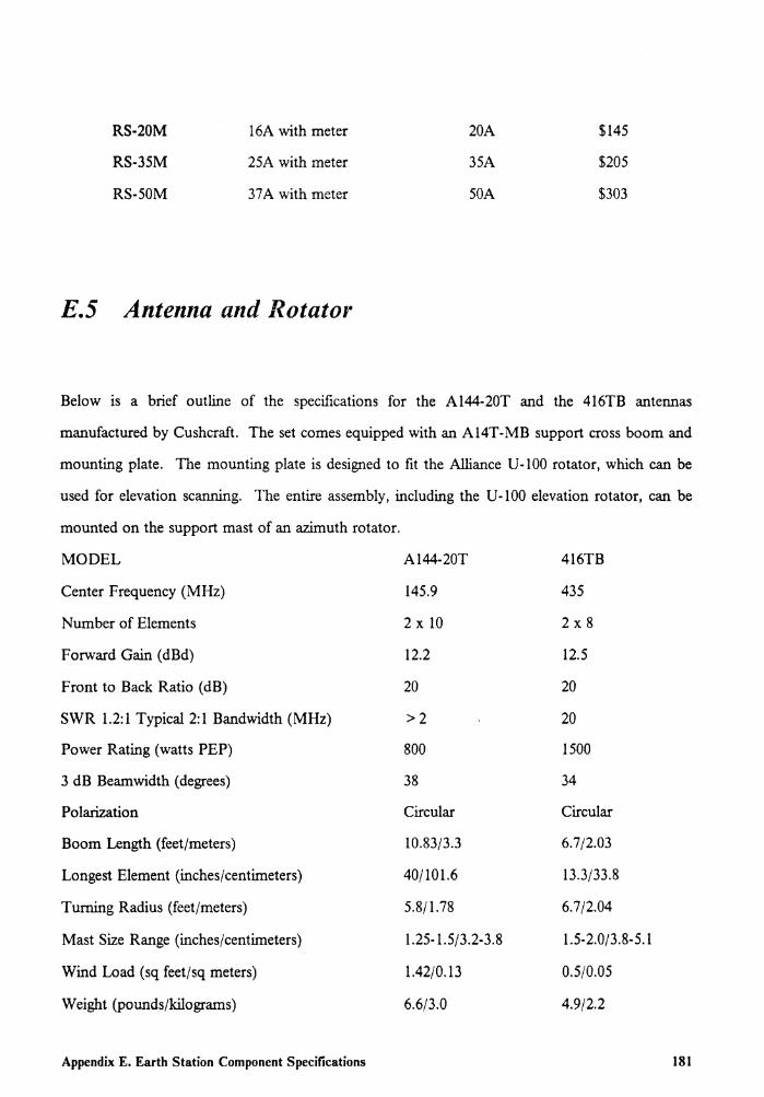
RS-20M

RS-35M

RS-SOM

l 6A with meter

25A with meter

37A with meter

E.5 Antenna and Rotator

20A

35A

50A

$145

$205

$303

Below is a brief outline of the specifications for the Al44-20T and the 416TB antennas

manufactured by Cushcraft. The set comes equipped with an Al4T-MB support cross boom and

mounting plate. The mounting plate is designed to fit the Alliance U-100 rotator, which can be

used for elevation scanning. The entire assembly, including the U-100 elevation rotator, can be

mounted on the support mast of an azimuth rotator.

MODEL Al44-20T 416TB

Center Frequency (MHz) 145.9 435

Number of Elements 2 x 10 2x8

Forward Gain (dBd) 12.2 12.5

Front to Back Ratio (dB) 20 20

SWR 1.2:1 Typical 2:1 Bandwidth (MHz) >2 20

Power Rating (watts PEP) 800 1500

3 dB Beam width (degrees) 38 34

Polarization Circular Circular

Boom Length (feet/meters) 10.83/3.3 6.7/2.03

Longest Element (inches/centimeters) 40/101.6 13.3/33.8

Turning Radius (feet/meters) 5.8/1.78 6.7/2.04

Mast Size Range (inches/centimeters) 1.25-1.5/3.2-3.8 1.5-2.0/3.8-5.1

Wind Load (sq feet/sq meters) 1.42/0.13 0.5/0.05

Weight (pounds/kilograms) 6.6/3.0 4.9/2.2


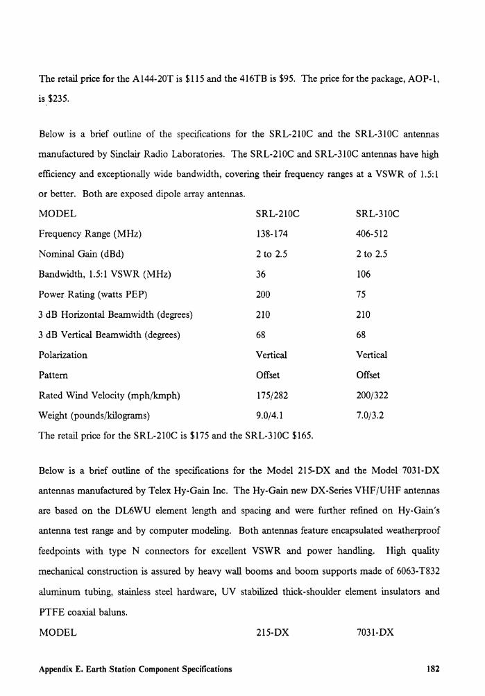
The retail price for the Al44-20T is $ll5 and the 416TB is $95. The price for the package, AOP-1,

is $235.

Below is a brief outline of the specifications for the SRL-210C and the SRL-310C antennas

manufactured by Sinclair Radio Laboratories. The SRL-210C and SRL-310C antennas have high

efficiency and exceptionally wide bandwidth, covering their frequency ranges at a VSWR of 1.5: 1

or better. Both are exposed dipole array antennas.

MODEL SRL-210C SRL-310C

Frequency Range (MHz) 138-174 406-512

Nominal Gain ( dBd) 2 to 2.5 2 to 2.5

Bandwidth, 1.5:1 VSWR (MHz) 36 106


3 dB Horizontal Beamwidth (degrees) 210 210

3 dB Vertical Beamwidth (degrees) 68 68

Polarization Vertical Vertical

Pattern Offset Offset

Rated Wind Velocity (mph/kmph) 175/282 200/322


The retail price for the SRL-210C is $175 and the SRL-310C $165.

Below is a brief outline of the specifications for the Model 215-DX and the Model 7031-DX

antennas manufactured by Telex Hy-Gain Inc. The Hy-Gain new DX-Series VHF/UHF antennas

are based on the DL6WU element length and spacing and were further refined on Hy-Gain's

antenna test range and by computer modeling. Both antennas feature encapsulated weatherproof

feedpoints with type N connectors for excellent VSWR and power handling. High quality

mechanical construction is assured by heavy wall booms and boom supports made of 6063-T832

aluminum tubing, stainless steel hardware, UV stabilized thick-shoulder element insulators and

PTFE coaxial baluns.

MODEL 215-DX 7031-DX


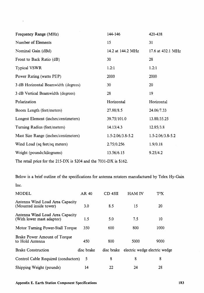
Frequency Range (MHz) 144-146 420-438

Number of Elements 15 31

Nominal Gain (dBd) 14.2 at 144.2 MHz 17.6 at 432.1 MHz

Front to Back Ratio (dB) 30 28

Typical VSWR 1.2:1 1.2: 1


3 dB Horizontal Beamwidth (degrees) 30 20

3 dB Vertical Beamwidth (degrees) 28 19

Polarization Horizontal Horizontal

Boom Length (feet/meters) 27.88/8.5 24.06/7.33

Longest Element (inches/centimeters) 39.75/101.0 13.88/35.25

Turning Radius (feet/meters) 14.13/4.3 12.85/3.8

Mast Size Range (inches/centimeters) 1.5-2.06/3.8-5.2 1.5-2.06/3.8-5.2

Wind Load (sq feet/sq meters) 2.75/0.256 1.9/0.18


The retail price for the 215-DX is $204 and the 7031-DX is $162.

Below is a brief outline of the specifications for antenna rotators manufactured by Telex Hy-Gain

Inc.

MODEL AR40 CD 4511 HAMIV T2X

Antenna Wind Load Area Capacity (Mounted inside tower) 3.0 8.5 15 20

Antenna Wind Load Area Capacity (With lower mast adaptor) 1.5 5.0 7.5 10

Motor Turning Power-Stall Torque 350 600 800 1000

Brake Power Amount of Torque to Hold Antenna 450 800 5000 9000

Brake Construction disc brake disc brake electric wedge electric wedge

Control Cable Required (conductors) 5 8 8 8

Shipping Weight (pounds) 14 22 24 28


Retail Price $221 $310 $440 $525


The vita has been removed from the scanned document

› bitstream › handle › 10919 › 74533 › ld5655.v855... · an analysis of low-earth-orbit...

Documents