a boundary-fragment-model for object detectionvgg/publications/papers/opelt06.pdf · a...

$: A Boundary-Fragment-Model for Object Detectionvgg/publications/papers/opelt06.pdf · A Boundary-Fragment-Model for Object Detection Andreas Opelt1, Axel Pinz1, ... a strong \Boundary-Fragment-Model"$
A Boundary-Fragment-Model for ObjectDetection

Andreas Opelt1, Axel Pinz1, and Andrew Zisserman2

1 Vision-based Measurement Group, Inst. of El. Measurement and Meas. Sign. Proc.Graz, University of Technology, Austria

{opelt, axel.pinz}@tugraz.at2 Visual Geometry Group, Department of Engineering Science

University of [email protected]

Abstract. The objective of this work is the detection of object classes,such as airplanes or horses. Instead of using a model based on salient im-age fragments, we show that object class detection is also possible usingonly the object’s boundary. To this end, we develop a novel learning tech-nique to extract class-discriminative boundary fragments. In addition totheir shape, these “codebook” entries also determine the object’s centroid(in the manner of Leibe et al. [19]). Boosting is used to select discrim-inative combinations of boundary fragments (weak detectors) to forma strong “Boundary-Fragment-Model” (BFM) detector. The generativeaspect of the model is used to determine an approximate segmentation.We demonstrate the following results: (i) the BFM detector is able torepresent and detect object classes principally defined by their shape,rather than their appearance; and (ii) in comparison with other publishedresults on several object classes (airplanes, cars-rear, cows) the BFMdetector is able to exceed previous performances, and to achieve thiswith less supervision (such as the number of training images).

1 Introduction and Objective

Several recent papers on object categorization and detection have explored theidea of learning a codebook of appearance parts or fragments from a corpus ofimages. A particular instantiation of an object class in an image is then composedfrom codebook entries, possibly arising from different source images. Examplesinclude Agarwal & Roth [1], Vidal-Naquet & Ullman [27], Leibe et al. [19], Fer-gus et al. [12, 14], Crandall et al. [9], Bar-Hillel et al. [3]. The methods differ onthe details of the codebook, but more fundamentally they differ in how strictlythe geometry of the configuration of parts constituting an object class is con-strained. For example, Csurka et al. [10], Bar-Hillel et al. [3] and Opelt et al. [22]simply use a “bag of visual words” model (with no geometrical relations betweenthe parts at all), Agarwal & Roth [1], Amores et al. [2], and Vidal-Naquet andUllman [27] use quite loose pairwise relations, whilst Fergus et al. [12] have astrongly parametrized geometric model consisting of a joint Gaussian over the

2 Andreas Opelt et al.

centroid position of all the parts. The approaches using no geometric relationsare able to categorize images (as containing the object class), but generally donot provide location information (no detection). Whereas the methods with evenloose geometry are able to detect the object’s location.

The method of Leibe et al. ([19], [20]) has achieved the best detection per-formance to date on various object classes (e.g. cows, cars-rear (Caltech)). Theirrepresentation of the geometry is algorithmic – all parts vote on the object cen-troid as in a Generalized Hough transform. In this paper we explore a similargeometric representation to that of Leibe et al. [19] but use only the boundariesof the object, both internal and external (silhouette). In our case the codebookconsists of boundary-fragments, with an additional entry recording the locationof the object’s centroid. Figure 1 overviews the idea. The boundary representsthe shape of the object class quite naturally without requiring the appearance(e.g. texture) to be learnt. For certain categories (bottles, cups) where the surfacemarkings are very variable, approaches relying on consistency of these appear-ances may fail or need considerable training data to succeed. Our method, withits stress on boundary representation, is highly suitable for such objects. Theintention is not to replace appearance fragments but to develop complementaryfeatures. As will be seen, in many cases the boundary alone performs as well asor better than the appearance and segmentation masks (mattes) used by otherauthors (e.g. [19, 27]) – the boundary is responsible for much of the success.

Original Image All matched boundaryfragments Centroid Voting on a subset of the matched fragments

Backprojected MaximumSegmentation / Detection

Fig. 1. An overview of applying the BF model detector.

The areas of novelty in the paper include: (i) the manner in which theboundary-fragment codebook is learnt – fragments (from the boundaries of thetraining objects) are selected to be highly class-distinctive, and are stable in theirprediction of the object centroid; and (ii) the construction of a strong detector(rather than a classifier) by Boosting [15] over a set of weak detectors built onboundary fragments. This detector means that it is not necessary to scan theimage with a sliding window in order to localize the object.

Boundaries have been used in object recognition to a certain extent: Ku-mar et al. [17] used part outlines in their application of pictorial structures [11];Fergus et al. [13] used boundary curves between bitangent points in their exten-sion of the constellation model; and, Jurie and Schmid [16] detected circular arc

Lecture Notes in Computer Science 3

features from boundary curves. However, in all these cases the boundary featuresare segmented independently in individual images. They are not flexibly selectedto be discriminative over a training set, as they are here. Bernstein and Amit [4]do use discriminative edge maps. However, theirs is only a very local representa-tion of the boundary; in contrast we capture the global geometry of the objectcategory. Recently, and independently, Shotton et al. [24] presented a methodquite related to the Boundary-Fragment-Model presented here. The principal dif-ferences are: the level of segmentation required in training ([24] requires more);the number of boundary fragments employed in each weak detector (a singlefragment in [24], and a variable number here); and the method of localizing thedetected centroid (grid in [24], mean shift here).

We will illustrate BFM classification and detection for a running example,namely the object class cows. For this we selected cow images as [7, 19] whichoriginate from the videos of Magee and Boyle [21]. The cows appear at variouspositions in the image with just moderate scale changes. Figure 2 shows some ex-ample images. Figure 3 shows detections using the BFM detector on additional,more complex, cow images obtained from Google image search.

Fig. 2. Example training images for the cows cat-egory.

Fig. 3. Examples of detectingmultiple objects in one test image.

2 Learning boundary fragments

In a similar manner to [19], we require the following data to train the model:

– A training image set with the object delineated by a bounding box.– A validation image set labelled with whether the object is absent or present,

and the object’s centroid (but the bounding box is not necessary).

The training images provide the candidate boundary fragments, and these can-didates are optimized over the validation set as described below. For the resultsof this section the training set contains 20 images of cows, and the validationset contains 25 cow images (the positive set) and 25 images of other objects(motorbikes and cars – the negative set).

Given the outlines of the training images we want to identify boundary frag-ments that:

(i) discriminate objects of the target category from other objects, and(ii) give a precise estimate of the object centroid.


A candidate boundary fragment is required to (i) match edge chains often in thepositive images but not in the negative, and (ii) have a good localization of thecentroid in the positive images. These requirements are illustrated in figure 4.The idea of using validation images for discriminative learning is motivated bySali and Ullman [23]. However, in their work they only consider requirement (i),the learning of class-discriminate parts, but not the second requirement which isa geometric relation. In the following we first explain how to score a boundaryfragment according to how well it satisfies these two requirements, and then howthis score is used to select candidate fragments from the training images.

Fig. 4. Scoring boundary fragments. The first row shows an example of a boundaryfragment that matches often on the positive images of the validation set, and less oftenon the negative images. Additionally it gives a good estimate of the centroid positionon the positive images. In contrast, the second row shows an example of an unsuitableboundary fragment. The cross denotes the estimate of the centroid and the asteriskthe correct object centroid.

2.1 Scoring a boundary fragment

Linked edges are obtained in the training and validation set using a Canny edgedetector with hysteresis. We do not obtain perfect segmentations – there maybe gaps and false edges. A linked edge in the training image is then consideredas a candidate boundary fragment γi, and scoring cost C(γi) is a product of twofactors:

1. cmatch(γi): the matching cost of the fragment to the edge chains in thevalidation images using a Chamfer distance [5, 6], see (1). This is describedin more detail below.

2. cloc(γi): the distance (in pixels) between the true object centroid and thecentroid predicted by the boundary fragment γi averaged over all the positivevalidation images.

with C(γi) = cmatch(γi)cloc(γi). The matching cost is computed as


cmatch(γi) =∑L+

i=1 distance(γi, Pvi)/L+

∑L−i=1 distance(γi, Nvi)/L−

(1)

where L− denotes the number of negative validation images Nvi and L+ thenumber of positive validation images Pvi

, and distance(γi, Ivi) is the distance to

the best matching edge chain in image Ivi :

distance(γi, Ivi) =

1|γi| min

γi⊂Ivi

∑t∈γi

DTIvi(t) (2)

where DTIviis the distance transform. The Chamfer distance [5] is implemented

using 8 orientation planes with an overlap of 5 degrees. The orientation of theedges is averaged over a length of 7 pixels by orthogonal regression. Becauseof background clutter the best match is often located on highly textured back-ground clutter, i.e. it is not correct. To solve this problem we use the N = 10best matches (with respect to (2)), and from these we take the one with the bestcentroid prediction. Note, images are scale normalized for training.

2.2 Selecting boundary fragments

Having defined the cost, we now turn to selecting candidate fragments. This isaccomplished by optimization. For this purpose seeds are randomly distributedon the boundary of each training image. Then at each seed we extract boundaryfragments. We let the size of each fragment grow and at every step we calculatethe cost C(γi) on the validation set. Figure 5(a) shows three examples of thisgrowing of boundary fragments (the length varies from 20 pixels in steps of30 pixels in both directions up to a length of 520 pixels). The cost is minimizedover the varying length of the boundary fragment to choose the best fragment.If no length variation meets some threshold of the cost we reject this fragmentand proceed with the next one. Using this procedure we obtain a codebook ofboundary fragments each having the geometric information to vote for an objectcentroid.

To reduce redundancy in the codebook the resulting boundary fragment setis merged using agglomerative clustering on medoids. The distance function isdistance(γi, γj) (where Ivi in (2) is replaced by the binary image of fragment γj)and we cluster with a threshold of thcl = 0.2. Figure 5(b) shows some examplesof resulting clusters. This optimized codebook forms the basis for the next stagein learning the BFM.

3 Training an object detector using Boosting

At this stage we have a codebook of optimized boundary fragments each carryingadditional geometric information on the object centroid. We now want to com-bine these fragments so that their aggregated estimates determine the centroidand increase the matching precision. In the case of image fragments, a single


(a) (b)

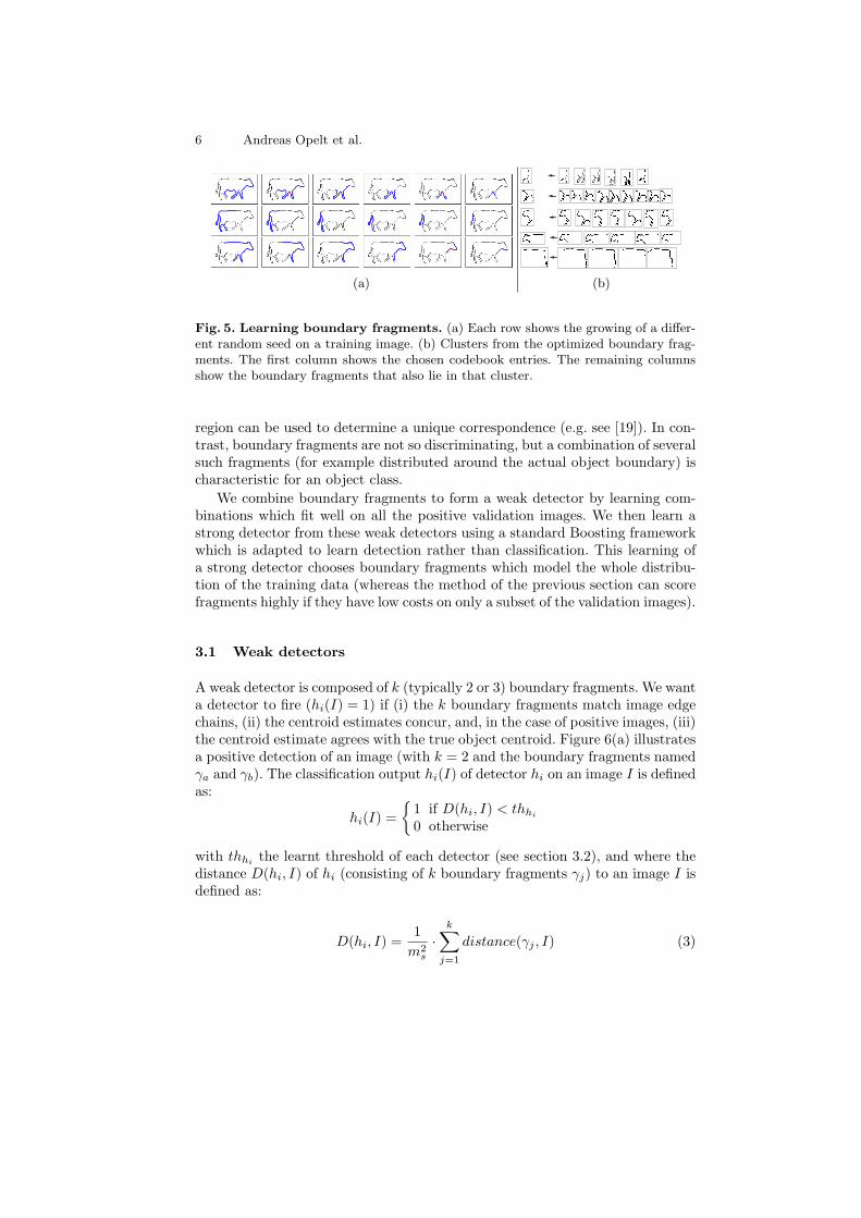
Fig. 5. Learning boundary fragments. (a) Each row shows the growing of a differ-ent random seed on a training image. (b) Clusters from the optimized boundary frag-ments. The first column shows the chosen codebook entries. The remaining columnsshow the boundary fragments that also lie in that cluster.

region can be used to determine a unique correspondence (e.g. see [19]). In con-trast, boundary fragments are not so discriminating, but a combination of severalsuch fragments (for example distributed around the actual object boundary) ischaracteristic for an object class.

We combine boundary fragments to form a weak detector by learning com-binations which fit well on all the positive validation images. We then learn astrong detector from these weak detectors using a standard Boosting frameworkwhich is adapted to learn detection rather than classification. This learning ofa strong detector chooses boundary fragments which model the whole distribu-tion of the training data (whereas the method of the previous section can scorefragments highly if they have low costs on only a subset of the validation images).

3.1 Weak detectors

A weak detector is composed of k (typically 2 or 3) boundary fragments. We wanta detector to fire (hi(I) = 1) if (i) the k boundary fragments match image edgechains, (ii) the centroid estimates concur, and, in the case of positive images, (iii)the centroid estimate agrees with the true object centroid. Figure 6(a) illustratesa positive detection of an image (with k = 2 and the boundary fragments namedγa and γb). The classification output hi(I) of detector hi on an image I is definedas:

hi(I) ={

1 if D(hi, I) < thhi

0 otherwise

with thhi the learnt threshold of each detector (see section 3.2), and where thedistance D(hi, I) of hi (consisting of k boundary fragments γj) to an image I isdefined as:

D(hi, I) =1

m2s

·k∑

j=1

distance(γj , I) (3)

Lecture Notes in Computer Science 7� � � � � � � � � � � � � � � � ��

� � � � � � � � � � � � � � � � � � � � � � � � � � � � � � � � � � � �

� � � � � � � � � � � � � � � � � � � � � � � �� ! � " # � � $ % ! � & " � ' ( # " � � � � ! $ ! ' � " � )* � � �� +�

�

(a) (b)

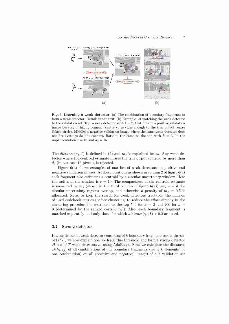
Fig. 6. Learning a weak detector. (a) The combination of boundary fragments toform a weak detector. Details in the text. (b) Examples of matching the weak detectorto the validation set. Top: a weak detector with k = 2, that fires on a positive validationimage because of highly compact centre votes close enough to the true object centre(black circle). Middle: a negative validation image where the same weak detector doesnot fire (votings do not concur). Bottom: the same as the top with k = 3. In theimplementation r = 10 and dc = 15.

The distance(γj , I) is defined in (2) and ms is explained below. Any weak de-tector where the centroid estimate misses the true object centroid by more thandc (in our case 15 pixels), is rejected.

Figure 6(b) shows examples of matches of weak detectors on positive andnegative validation images. At these positions as shown in column 2 of figure 6(a)each fragment also estimates a centroid by a circular uncertainty window. Herethe radius of the window is r = 10. The compactness of the centroid estimateis measured by ms (shown in the third column of figure 6(a)). ms = k if thecircular uncertainty regions overlap, and otherwise a penalty of ms = 0.5 isallocated. Note, to keep the search for weak detectors tractable, the numberof used codebook entries (before clustering, to reduce the effort already in theclustering procedure) is restricted to the top 500 for k = 2 and 200 for k =3 (determined by the ranked costs C(γi)). Also, each boundary fragment ismatched separately and only those for which distance(γj , I) < 0.2 are used.

3.2 Strong detector

Having defined a weak detector consisting of k boundary fragments and a thresh-old thhi , we now explain how we learn this threshold and form a strong detectorH out of T weak detectors hi using AdaBoost. First we calculate the distancesD(hi, Ij) of all combinations of our boundary fragments (using k elements forone combination) on all (positive and negative) images of our validation set


I1 . . . Iv. Then in each iteration 1 . . . T we search for the weak detector that ob-tains the best detection result on the current image weighting (for details seeAdaBoost [15]). This selects weak detectors which generally (depending on theweighting) “fire” often on positive validation images (classify them as correctand estimate a centroid closer than dc to the true object centroid) and not onthe negative ones. Figure 7 shows examples of learnt weak detectors that con-tribute to the strong detector. Each of these weak detectors also has a weightwhi

. The output of a strong detector on a whole test image is then:

H(I) = sign(T∑

i=1

hi(I) · whi). (4)

The sign function is replaced in the detection procedure by a threshold tdet,where an object is detected in the image I if H(I) > tdet and no evidence for theoccurrence of an object if H(I) ≤ tdet (the standard formulation uses tdet = 0).

Fig. 7. Examples of weak detectors, left for k = 2, and right for k = 3.

4 Object Detection

Detection algorithm and segmentation: The steps of the detection algo-rithm are now described and qualitatively illustrated in figure 8. First the edgesare detected (step 1) then the boundary fragments of the weak detectors, thatform the strong detector, are matched to this edge image (step 2). In order to de-tect (one or more) instances of the object (instead of classifying the whole image)each weak detector hi votes with a weight whi in a Hough voting space (step 3).Votes are then accumulated in a circular search window (W (xn)) with radius dc

around candidate points xn (represented by a Mean-Shift-Mode estimation [8]).The Mean-Shift modes that are above a threshold tdet are taken as detectionsof object instances (candidate points). The confidence in detections at thesecandidate points xn is calculated using probabilistic scoring (see below). Thesegmentation is obtained by backprojection of the boundary fragments (step3) of weak detectors which contributed to that centre to a binary pixel map.Typically, the contour of the object is over-represented by these fragments. Weobtain a closed contour of the object, and additional, spurious contours (seen infigure 8, step 3). Short segments (< 30 pixels) are deleted, the contour is filled(using Matlab’s ‘filled area’ in regionprops), and the final segmentation matte isobtained by a morphological opening, which removes thin structures (votes fromoutliers that are connected to the object). Finally, each of the objects obtainedby this procedure is represented by its bounding box.

Lecture Notes in Computer Science 9� � � � � � � � � � � � � � � � � � � � � �� ! " # $ ! % � & ' ( ) * ' + ) � , - . � $ / -

0 � � � � � � � � � � �� ! " # $ ! % � & ' ( ) * ' + ) � , - . � $ / -

1 2 3 4 5 6 78 3 2 3 9 2 : ; < = : > ? @ > A @ > B @ > C @

Fig. 8. Examples of processing test images with the BFM detector.

Probabilistic scoring: At candidate points xn for instances of an objectcategory c, found by the strong detector in the test image IT we sum up the(probabilistic) votings of the weak detectors hi in a 2D Hough voting space whichgives us the probabilistic confidence:

conf(xn) =T∑

i

p(c, hi) =T∑

i

p(hi)p(c|hi) (5)

where p(hi) = 1∑M

q=1score(hq,IT )

· score(hi, IT ) describes the pdf of the effective

matching of the weak detector with score(hi, IT ) = 1/D(hi, IT ) (see (3)). Thesecond term of this vote is the confidence we have in each specific weak detectorand is computed as:

p(c|hi) =#firescorrect

#firestotal(6)

where #firescorrect is the number of positive and #firestotal is the number ofpositive and negative validation images the weak detector fires on. Finally ourconfidence of an object appearing at position xn is computed by using a Mean-Shift algorithm [8] (circular window W (xn)) in the Hough voting space definedas: conf(xn|W (xn)) =

∑Xj∈W (xn) conf(Xj).

5 Detection Results

In this section we compare the performance of the BFM detector to publishedstate-of-the-art results, and also give results on new data sets. Throughout weuse fixed parameters (T = 200, k = 2, tdet = 8) for our training and testingprocedure unless stated otherwise. An object is deemed correctly detected if theoverlap of the bounding boxes (detection vs ground truth) is greater than 50%.


Cows: First we give quantitative results on the cow dataset. We used 20training images (validation set 25 positive/25 negative) and tested on 80 un-seen images, half belonging to the category cows and half to counter examples(cars and motorbikes). In table 2 we compare our results to those reported byLeibe et al. [19] and Caputo et al. [7] (Images are from the same test set –though the authors do not specify which ones they used). We perform as wellas the result in [19], clearly demonstrating that in some cases the contour aloneis sufficient for excellent detection performance. Kumar et al. [17] also give anRPC curve for cow detection with an ROC-equal-error rate of 10% (though theyuse different test images). Note, that the detector can identify multiple instancesin an image, as shown in figure 3.

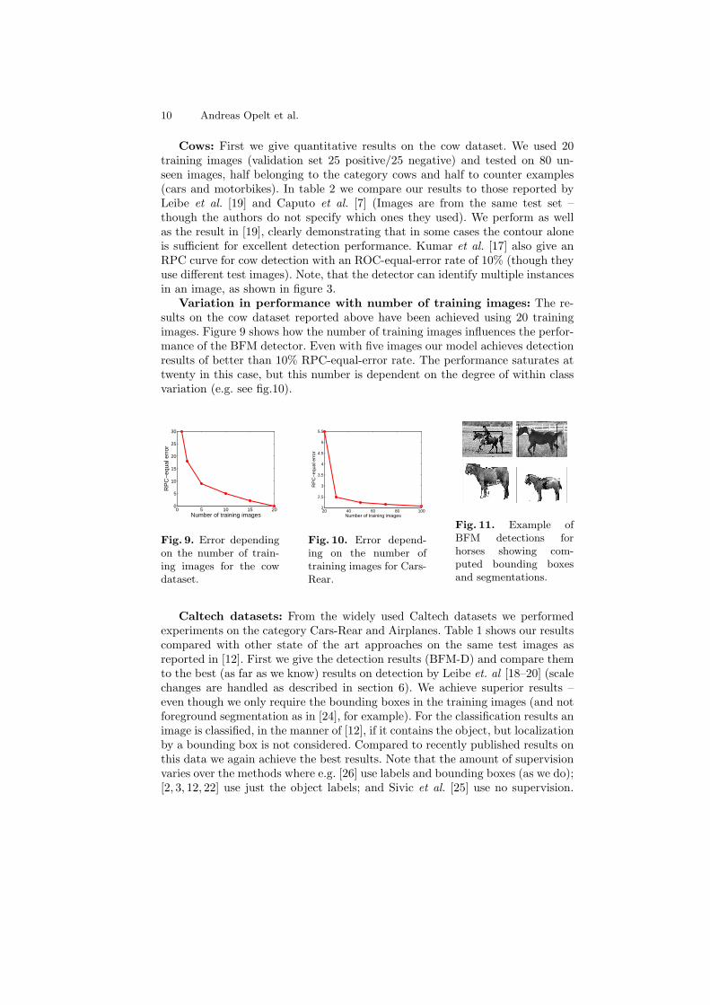
Variation in performance with number of training images: The re-sults on the cow dataset reported above have been achieved using 20 trainingimages. Figure 9 shows how the number of training images influences the perfor-mance of the BFM detector. Even with five images our model achieves detectionresults of better than 10% RPC-equal-error rate. The performance saturates attwenty in this case, but this number is dependent on the degree of within classvariation (e.g. see fig.10).

0 5 10 15 200

5

10

15

20

25

30

Number of training images

RP

C−

equa

l err

or

Fig. 9. Error dependingon the number of train-ing images for the cowdataset.

20 40 60 80 1002

2.5

3

3.5

4

4.5

5

5.5

Number of training images

RP

C−

equa

l err

or

Fig. 10. Error depend-ing on the number oftraining images for Cars-Rear.

Fig. 11. Example ofBFM detections forhorses showing com-puted bounding boxesand segmentations.

Caltech datasets: From the widely used Caltech datasets we performedexperiments on the category Cars-Rear and Airplanes. Table 1 shows our resultscompared with other state of the art approaches on the same test images asreported in [12]. First we give the detection results (BFM-D) and compare themto the best (as far as we know) results on detection by Leibe et. al [18–20] (scalechanges are handled as described in section 6). We achieve superior results –even though we only require the bounding boxes in the training images (and notforeground segmentation as in [24], for example). For the classification results animage is classified, in the manner of [12], if it contains the object, but localizationby a bounding box is not considered. Compared to recently published results onthis data we again achieve the best results. Note that the amount of supervisionvaries over the methods where e.g. [26] use labels and bounding boxes (as we do);[2, 3, 12, 22] use just the object labels; and Sivic et al. [25] use no supervision.


It should be pointed out, that we use just 50 training images and 50 validationimages for each category, which is less than the other approaches use. Figure10 shows the error rate depending on the number of training images (again, thesame number of positive and negative validation images are used). However, it isknown that the Caltech images are now not sufficiently demanding, so we nextconsider further harder situations.

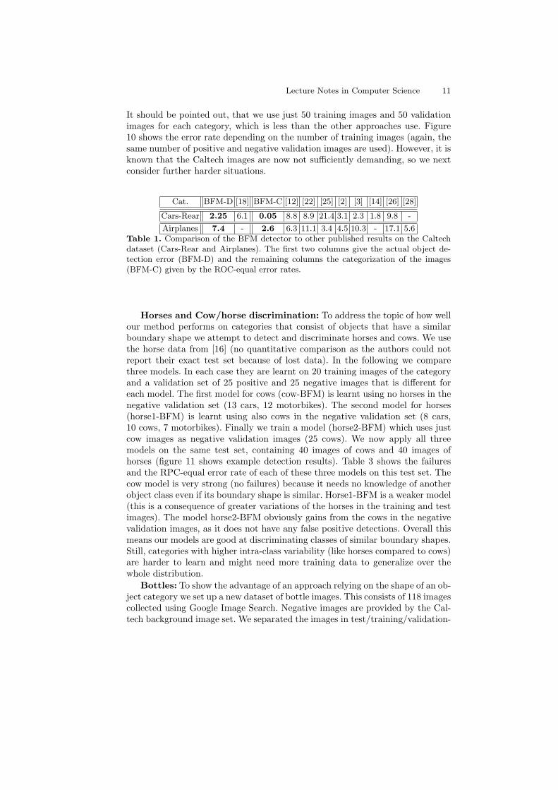
Cat. BFM-D [18] BFM-C [12] [22] [25] [2] [3] [14] [26] [28]

Cars-Rear 2.25 6.1 0.05 8.8 8.9 21.4 3.1 2.3 1.8 9.8 -

Airplanes 7.4 - 2.6 6.3 11.1 3.4 4.5 10.3 - 17.1 5.6Table 1. Comparison of the BFM detector to other published results on the Caltechdataset (Cars-Rear and Airplanes). The first two columns give the actual object de-tection error (BFM-D) and the remaining columns the categorization of the images(BFM-C) given by the ROC-equal error rates.

Horses and Cow/horse discrimination: To address the topic of how wellour method performs on categories that consist of objects that have a similarboundary shape we attempt to detect and discriminate horses and cows. We usethe horse data from [16] (no quantitative comparison as the authors could notreport their exact test set because of lost data). In the following we comparethree models. In each case they are learnt on 20 training images of the categoryand a validation set of 25 positive and 25 negative images that is different foreach model. The first model for cows (cow-BFM) is learnt using no horses in thenegative validation set (13 cars, 12 motorbikes). The second model for horses(horse1-BFM) is learnt using also cows in the negative validation set (8 cars,10 cows, 7 motorbikes). Finally we train a model (horse2-BFM) which uses justcow images as negative validation images (25 cows). We now apply all threemodels on the same test set, containing 40 images of cows and 40 images ofhorses (figure 11 shows example detection results). Table 3 shows the failuresand the RPC-equal error rate of each of these three models on this test set. Thecow model is very strong (no failures) because it needs no knowledge of anotherobject class even if its boundary shape is similar. Horse1-BFM is a weaker model(this is a consequence of greater variations of the horses in the training and testimages). The model horse2-BFM obviously gains from the cows in the negativevalidation images, as it does not have any false positive detections. Overall thismeans our models are good at discriminating classes of similar boundary shapes.Still, categories with higher intra-class variability (like horses compared to cows)are harder to learn and might need more training data to generalize over thewhole distribution.

Bottles: To show the advantage of an approach relying on the shape of an ob-ject category we set up a new dataset of bottle images. This consists of 118 imagescollected using Google Image Search. Negative images are provided by the Cal-tech background image set. We separated the images in test/training/validation-


Method RPC-err.

Caputo et al. [7] 2.9%

Leibe et al. [19] 0.0%

Our approach 0.0%Table 2. Comparison of theBFM detector to other pub-lished results on the cows.

- cow horse1 horse2

FP 0 3 0

FN 0 13 12

M 0 1 2

RPC-err 0% 23% 19%Table 3. The first 3 rows show the failures madeby the three different models (FP=false positive,FN=false negative, M=multiple detection). The lastrow shows the RPC-equal-error rate for each model.

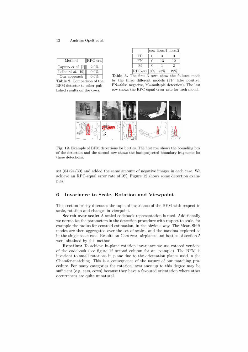
Fig. 12. Example of BFM detections for bottles. The first row shows the bounding boxof the detection and the second row shows the backprojected boundary fragments forthese detections.

set (64/24/30) and added the same amount of negative images in each case. Weachieve an RPC-equal error rate of 9%. Figure 12 shows some detection exam-ples.

6 Invariance to Scale, Rotation and Viewpoint

This section briefly discusses the topic of invariance of the BFM with respect toscale, rotation and changes in viewpoint.

Search over scale: A scaled codebook representation is used. Additionallywe normalize the parameters in the detection procedure with respect to scale, forexample the radius for centroid estimation, in the obvious way. The Mean-Shiftmodes are then aggregated over the set of scales, and the maxima explored asin the single scale case. Results on Cars-rear, airplanes and bottles of section 5were obtained by this method.

Rotation: To achieve in-plane rotation invariance we use rotated versionsof the codebook (see figure 12 second column for an example). The BFM isinvariant to small rotations in plane due to the orientation planes used in theChamfer-matching. This is a consequence of the nature of our matching pro-cedure. For many categories the rotation invariance up to this degree may besufficient (e.g. cars, cows) because they have a favoured orientation where otheroccurrences are quite unnatural.


Changes in viewpoint: For natural objects (e.g. cows) the perceived bound-ary is the visual rim. The position of the visual rim on the object will vary withpose but the shape of the associated boundary fragment will be valid over arange of poses. We performed experiments under controlled conditions on theETH-80 database. With a BFM learnt for a certain aspect we could still de-tect a prominent mode in the Hough voting space up to 45 degrees rotation inboth directions (horizontal and vertical). Thus, to extend the BFM to variousaspects this invariance to small viewpoint changes reduces the number of neces-sary positions on the view-sphere to a handful of aspects that have to be trainedseparately. Our probabilistic formulation can be straightforwardly extended tomultiple aspects.

7 Discussion and Conclusions

We have described a Boundary Fragment Model for detecting instances of objectcategories. The method is able to deal with the partial boundaries that typicallyare recovered by an edge detector. Its performance is similar to or outperformsstate-of-the-art methods that include image appearance region fragments. Forclasses where the texture is very variable (e.g. bottles, mugs) a BFM may bepreferable. In other cases a combination of appearance and boundary will havesuperior performance.

It is worth noting that the BFM once learnt can be implemented very effi-ciently using the low computational complexity method of Felzenszwalb & Hut-tenlocher [11].

Currently our research is focusing on extending the BFM to multi-class andmultiple aspects of one class.

Acknowledgements

This work was supported by the Austrian Science Foundation FWF, projectS9103-N04, ECVision and Pascal Network of Excellence.

References

1. S. Agarwal, A. Awan, and D. Roth. Learning to detect objects in images via asparse, part-based representation. IEEE PAMI, 26(11):1475–1490, Nov. 2004.

2. J. Amores, N. Sebe, and P. Radeva. Fast spatial pattern discovery integratingboosting with constellations of contextual descriptors. In Proc. CVPR, volume 2,pages 769–774, CA, USA, June 2005.

3. A. Bar-Hillel, T. Hertz, and D. Weinshall. Object class recognition by boosting apart-based model. In Proc. CVPR, volume 2, pages 702–709, June 2005.

4. E. J. Bernstein and Y. Amit. Part-based statistical models for object classificationand detection. In Proc. CVPR, volume 2, pages 734–740, 2005.

5. G. Borgefors. Hierarchical chamfer matching: A parametric edge matching algo-rithm. IEEE PAMI, 10(6):849–865, 1988.


6. H. Breu, J. Gil, D. Kirkpatrick, and M. Werman. Linear time Euclidean distancetransform algorithms. IEEE PAMI, 17(5):529–533, May. 1995.

7. B. Caputo, C. Wallraven, and M. Nilsback. Object categorization via local kernels.In Proc. ICPR, pages 132–135, 2004.

8. D. Comaniciu and P. Meer. Mean shift: A robust approach towards feature spaceanalysis. In IEEE PAMI, volume 24(5), pages 603–619, 2002.

9. D. Crandall, P. Felzenszwalb, and D. Huttenlocher. Spatial priors for part-basedrecognition using statistical models. In Proc. CVPR, pages 10–17, 2005.

10. G. Csurka, C. Bray, C. Dance, and L. Fan. Visual categorization with bags ofkeypoints. In ECCV04. Workshop on Stat. Learning in Computer Vision, pages59–74, 2004.

11. P. Felzenszwalb and D. Huttenlocher. Pictorial structures for object recognition.Intl. Journal of Computer Vision, 61(1):55–79, 2004.

12. R. Fergus, P. Perona, and A. Zisserman. Object class recognition by unsupervisedscale-invariant learning. In Proc. CVPR, pages 264–271, 2003.

13. R. Fergus, P. Perona, and A. Zisserman. A visual category filter for google images.In Proc. ECCV, pages 242–256, 2004.

14. R. Fergus, P. Perona, and A. Zisserman. A sparse object category model for efficientlearning and exhaustive recognition. In Proc. Proc. CVPR, 2005.

15. Y. Freund and R. Schapire. A decision theoretic generalisation of online learning.Computer and System Sciences, 55(1):119–139, 1997.

16. F. Jurie and C. Schmid. Scale-invariant shape features for recognition of objectcategories. In Proc. of CVPR, pages 90–96, 2004.

17. M. Kumar, P. Torr, and A. Zisserman. Extending pictural structures for objectrecognition. In Proc. BMVC, 2004.

18. B. Leibe. Interleaved Object Categorization and Segmentation. PhD thesis, SwissFederal Institute of Technology, 2004.

19. B. Leibe, A. Leonardis, and B. Schiele. Combined object categorization and seg-mentation with an implicit shape model. In ECCV04. Workshop on Stat. Learningin Computer Vision, pages 17–32, May 2004.

20. B. Leibe and B. Schiele. Scale-invariant object categorization using a scale-adaptivemean-shift search. In DAGM’04, pages 145–153, Aug. 2004.

21. D. Magee and R. Boyle. Detecting lameness using re-sampling condensationand multi-steam cyclic hidden markov models. Image and Vision Computing,20(8):581–594, 2002.

22. A. Opelt, M. Fussenegger, A. Pinz, and P. Auer. Weak hypotheses and boostingfor generic object detection and recognition. In Proc. ECCV, pages 71–84, 2004.

23. E. Sali and S. Ullman. Combining class-specific fragments for object classification.In Proc. BMVC, pages 203–213, 1999.

24. J. Shotton, A. Blake, and R. Cipolla. Contour-based learning for object detection.In Proc. ICCV, pages 503–510, 2005.

25. J. Sivic, B. Russell, A. Efros, A. Zisserman, and W. Freeman. Discovering objectsand their location in images. In Proc. ICCV, 2005.

26. J. Thureson and S. Carlsson. Appearance based qualitative image description forobject class recognition. In Proc. ECCV, pages 518–529, 2004.

27. M. Vidal-Naquet and S. Ullman. Object recognition with informative features andlinear classification. In Proc. ICCV, volume 1, pages 281–288, 2003.

28. W. Zhang, B. Yu, G. Zelinsky, and D. Samaras. Object class recognition usingmultiple layer boosting with heterogenous features. In Proc. CVPR, pages 323–330, 2005.

a boundary-fragment-model for object detectionvgg/publications/papers/opelt06.pdf · a...

Documents