TICAM REPORT 96-36August 1996

A Boussinesq System for Two-Way Propagation ofNonlinear Dispersive Waves

Jerry L. Bona, and Min Chen

A BOUSSINESQ SYSTEM FOR TWO-WAYPROPAGATION OF NONLINEAR DISPERSIVE WAVES

JERRY L. BONADepartment of Mathematics and

Texas Institute for Computational and Applied MathematicsThe University of Texas, Austin, TX 78712 U.S.A.

MIN CHENDepartment of Mathematics

The Pennsylvania State UniversityUniversity Park, PA 16802 U.S.A.

ABSTRACT.

(1)

In this report, we study the system

1Nt + Wx + (NW)x - -Nxxt = 0,

61

Wt + Nx + WWx - - Wxxt = 0,6

which describes approximately the two-dimensional propagation of surface waves ina uniform horizontal channel of length Lo filled with an irrotational, incompressible,invisid fluid which in its undisturbed state has depth h. The non-dimensional vari-ables N(x, t) and W(x, t) represent, respectively, the deviation of the water surface

from its undisturbed position and the horizontal velocity at water level Ifh. Thenatural initial-boundary-value problem corresponding to the situation wherein thechannel is fitted with a wave-maker at both ends is formulated and analyzed theoret-ically. We then present a numerical algorithm for the approximation of solutions ofthe system (1) and prove the algorithm is fourth-order accurate both in time and inspace, is unconditionally stable, and has optimal computational complexity, which isto say the operation cost per time step is of order M with M being the number ofgrid points in the spatial discretization. Afterward, we implement the algorithm as acomputer code and use it to study head-on collisions of solitary waves. Our numer-ical simulation are compared with existing theoretical, numerical and experimentalresults. We have tentatively concluded that the system (1) is a good candidate formodeling two-dimensional surface water waves.

Keywords: Boussinesq systems, solitary waves, two-way propagation of waterwaves.

1. Introduction.Consideration is given to the propagation of waves in a uniform horizontal chan-

nel of length Lo filled to a depth h with an incompressible perfect fluid. Assum-ing the wave motion is generated irrotationally and that it is uniform across the

Typeset by AMS- TEX

width of the channel, the two-dimensional Euler equations are the full equationsof motion. Even the two-dimensional version of the Euler equations are currentlychallenging both theore~ically and with respect to the numerical approximation ofsolutions. Consequently, when the practical need arises to model waves, furtherapproximations are often made. Assuming that the maximum deviation a of thefree surface from its undisturbed position is small relative to h (small-amplitudewaves), that the typical wavelength A is large relative to h (long waves), and thatthe Stokes number S = aA 2/ h3 is of order one, the Euler equations may be formallyapproximated by the system (see Bona, Saut and Toland [6])

{

h2T/t - (jT/xxt = -hwx - (T/w)x

(2) h2 _ for (x, t) E n = [0,Lo] x [0,To].Wt - -Wxxt - -gT/x - WWx6

The independent variable x corresponds to distance along the channel with x = 0at the left-hand boundary, while t is the elapsed time. The dependent variable

W = w(x, t) is the horizontal velocity at water level fih at the location x alongthe channel at time t, T/ = T/(x, t) is similarly the deviation of the free surfacerelative to its undisturbed position and g is the acceleration of gravity. The system(2) has the same formal status as the classical Boussinesq system (see Boussinesq[8]) which means that they are both correct to the first order with respect to thesmall parameter € = a/h. To simplify the notation in the rest of the paper, we willuse the standard non-dimensional variables, x = x/h, i = t/y'h/g, N = T//h, andW = W / Co, where Co = yIgTi. The corresponding scaled Boussinesq system is

(3){

N'-iN .. , ~ -Wi - (NW).

Wi-6Wxxi = -Nj; - WWj;for(x, i) E n = [0, L] x [0, T],

where L = Lo/h and T = To/ Jh19.In this report, attention will be directed to the initial- and boundary-value prob-

lem for which there is specified

(4)

N(O, i) = hI (i),W(O, i) = VI (i),N(x,O) = h(x),

N(L, i) = h2(i),

W(L, i) = v2(i),W(x, 0) = 12(x).

The consistency requirements for the initial- and boundary-conditions are the ob-vious ones dictated by continuity considerations, namely

(5)hI(O) = h(O),VI (0) = 12(0),

h2 (0) = h(L ) ,

V2(0) = 12(£)·

The plan of the paper is as follows. In Section 2, the initial-boundary-valueproblem (3)-(4) is written as a system of integral equations. Existence, uniqueness,

2

(6)

and regularity results for the solutions of (3)-(4)-(5) are established by recourse tothe integral equations. A numerical algorithm having optimal order of efficiencyfor the approximation of solutions of (3)-(4)-(5) is then proposed in Section 3. Thescheme is based on the system of integral equations. In Section 4, it is shownthat the numerical scheme is unconditionally stable and fourth-order convergent inboth space and time. The algorithm is then implemented as a computer code andthe rate of convergence tested in Section 5. Numerical simulation of the head-oncollision of solitary waves are also presented in this section. The paper concludeswith a brief summary.

2. Theoretical Results.In this section, we prove that corresponding to given compatible initial- and

boundary-data as in (4)-(5), there exists an unique solution to (3)-(4), definedat least on [0,L] x [0,T] for some T > 0, and we examine the regularity of thissolution. The existence of a solution is established by converting (3)-(4) into integralequations and applying the contraction-mapping principle. The regularity thenfollows from the fact that solutions of the integral equations are exactly as smoothas the data affords. The argument is similar to that proposed in Bona and Dougalis[3] and in Benjamin, Bona and Mahony [2] for a single equation which modelsunidirectional waves and in Bona and Smith [7] for the pure initial-value problemfor another Boussinesq-type system (see also Bona et al. [6]). In what follows, wedrop the carets adorning the independent variables in (3).

To begin, write the system (3) in the form

(1 - a-28;)Nt = -Wx - (NW)x,

(1 - a-28;)Wt = -Nx - WWx,

where a2 = 6. Inverting the operator 1-a-28; subject to the boundary conditionsin (4), one obtains

Nt(x, t) = 1L G(x, s)( -Ws - (NW)s)ds + S(L - x)h~ + S(x)h~,

Wt(x, t) = 1£G(x, s)( -N, - WW,)ds + S(L - xlv; + S(x)v;,

whereG(x s) = _~cosh(a(L - x - s)) - cosh(a(L - Ix - sl))

'2 sinh(aL)and

S(x) = sinh(ax) .sinh(aL)

Since G(x, s) is continuous with respect to s, continuously differentiable except ats = x, and G(x, L) = G(x, 0) = 0 for all x E [0,L], the integrals on the right-handsides may be integrated by parts, thereby leading to

Nt = 1LK(x, s)(W + NW)ds + S(L - x)h~ + S(x)h~ _ FI(x, t, N, W),

Wt = 1LK(x, s)(N + ~W2)ds + S(L - x)v~ + S(x)v~ F2(x, t, N, W),

3

with8G a2

K (x, s) = !1 = - (S (L - x - s) + sign( x - s) S (L - Ix - s I)) .uS 2

Now integrating the equations in (6) with respect to the temporal variable, oneobtains

(7)

N(x, t) = fI(x) + 1t 1L K(x, s)(W + NW)dsdT

+ S(L - x)(hI(t) - hI(O)) + S(x)(h2(t) - h2(0)),

ltlL

1W(x, t) = 12(x) + K(x, s)(N + - WW)dsdT002

+ S(L - X)(VI(t) - VI(O)) + S(X)(V2(t) - V2(0)).

Note that any classical solution of (3)-(4) satisfies the integral equations in (7) sinceall the steps followed in the derivation of (7) may then be justified.

Denote by Ck(a, b) the Banach space of k-times continuously differentiable func-tions defined on [a,b], equipped with the norm

We will systematically abbreviate Ilfllco by Ilfll.Before presenting the local uniqueness result, it is convenient to prove some

properties of the mapping M defined by

(8) M(v)(x) = 1L K(x, s)v(s)ds

for any v E C(O, L)

Lemma 1. There is a constant CI depending only on L and constants Dk, k =0,1, ... , depending on k and L such that

(aJ if Aj = sUPO:<;x:<;L {J; IKY)(x, s)lds + JxL IKY)(x, s)lds}, j 2: 0, then

and(bJ if v E Ck(O,L) for some k 2: 0, then M(v) E Ck+I(O,L) and

In (aJ, KY) connotes the lh partial derivative of K with respect to x, computedclassically on the intervals [0, x] and [x, L].

Proof. Observing that for Ixl ::::;L, IS(x)1 ::::;1 and that K(x, s) is continuous in sexcept at s = x where there is a jump discontinuity with

(9)

4

one easily obtains that IK(x, s)1 ::::;2a2 which yields that Ao is bounded by theconstant 2a2 L. Since for Ixl ::::;L, IS'(x)1 is bounded by a constant depending onlyon L, and K~ is continuous, it is seen that At is bounded by a constant which alsodepends only on L. It is easy to verify that for x =I=- s,

(10)

which yields (a) for j 2: 0 with CI being any constant which bounds Ao and AI.

Let v E C(O, L) and denote M(v) by ¢. Using part (a), one sees that

II¢II::::; sup (L IK(x, s)ldsllvil ::::;clllvil.O:<;x:<;L Jo

Using (9) and (10), one shows that

¢'(x) = 1LK~(x, s)v(s)ds + 6v(x),

and that¢(m+2)(X) = 6¢(m) (x) + 6v(m+I)(x), for m 2: O.

The first equation yields ¢ E CI in the case v E CO with

II¢(x)llcl ~ (CI + 6)llvll,and the second equation, when used as the basis for an inductive argument, yields(b) for any k 2: O. 0

For any Banach space X (for instance X = Ck), the space C(O, T; X) is theBanach space of continuous maps u : [0, T] -+ X with the norm

Ilu!!C(O,TjX) = sup IIu(t)\\x.O<t<T

The product space X x X will be abbreviated by X2; it carries the norm

IIfllx = max{ IliI IIx, 1112IIx}

for f = (iI, h)·We are now ready to prove the local existence and global uniqueness of solutions

of the system of integral equations (7) corresponding to specified auxiliary data asin (4).

Theorem 2. Letf= (iI, h) E C(0,L)2, h= (hI,h2),v= (VI,V2) E C(0,T)2 forsome T, L> O. Suppose f, h and v to satisfy the compatibility conditions (5). De-fine Ilfll = max{llhllc(o,L), 1I12llc(o,L)}, Ilhll = max{lIhlllc(o,T), Ilh21Ic(0,T)}, andIIvll = max{llvIilc(o,T), Ilv2I1c(0,T)}. Then there is a To = To(T, L, 1 if II, "hll, "vII)::::;T and an unique solution pair (N, W) in C(O, To; C(O, L))2 that satisfies (7).Moreover, for any TI ::::;T, there is at most one solution of (7) in C(O, TI; C(O, L))2.

Proof. Let C = C(O, To; C(O, L))2 and write the pair of integral equations in (7)in the tidy form

v=Av.

5

We will show that the operator A defined by the right-hand side of (7) has a fixedpoint in C for suitably chosen To by using the contraction-mapping theorem. FromLemma 1 and the compatibility conditions, we see that if vE C, then Av E C.Suppose now that both v and w lie in the closed ball BR of radius R about 0 in C;then we have the helpful inequality

(11)(TO

IIAw(x, t) - Av(x, t)11e ::::;cI(l + IIvlle + IIwlle) Jo

Ilv - wllcdT

::::;cITo(l + 2R)llv - wllc == 811v - wllc.

If 8 < 1, then A is a contraction mapping. For v E BR, let B denote the terms in(7) involving the initial- and boundary-values, namely

It is obvious that IIBllc(0,TjC(0,L))2 ~ b lifll + 2(llhll + Ilvl\), and therefore

IIAvl1e = IjAv - AO + Bile ::;811vllc + IIBIIe ::::;8R + b.

Thus if we choose R = 2b and To = To(b) = ?(LL~P\~. , it is seen that

18 ="2 and IIAvllc::::; R.

The contraction-mapping theorem can be applied to establish the local existenceof a solution of (7).

For uniqueness, let h = v - w where v and ware two solutions of (7) inC = C(0,TI;C(0,L))2. As in (11), one can show that

for 0 ::::;t ::::;TI, where C depends on both Ilvllc and Ilwlle. Gronwall's Lemma thenimplies that

Ilhlle = 0,

which finishes the proof of the theorem. 0

Theorem 3. (RegularityJ Let f = (iI, h) E C2(0, L)2, h = (hI, h2), v = (VI, V2) ECI(0,T)2 for some T, L > 0 satisfy the compatibility condit'ions (5). Then anysolution pair (N, W) in C(0,To;C(0,L))2 of (7) lies in CI(0,To;C2(0,L))2 and isa classical solution of the initial- and boundary-value problem (3) on the interval[0, To}.

Proof. Since U (N, W) has continuous component functions, one shows by usingLemma l(b) that AU is differentiable with respect to t, whence Ut exists and is

6

given by (6). Since h' and v' E CO(O, T)2, it transpires that Ut E C. Rewrite (7)as

where M is defined in (8). Lemma 1 yields that the terms on the right-hand side ofthe latter equations are in CI(O, To; CI(O, L)), which is equivalent to saying that Nand Ware in C1(0, To; CI(O, L)). Using the same argument once more gives that(N, W) E CI(O, To; C2(0, L))2.

Using (7) again shows that (4) is valid because S(O) = 0, S(L) = 1, and K(O, s) =K(L, s) = O. That the solution of (7) satisfies (3) can be established by observingthe derivation leading from (3) to (7) is reversible if (N, W) E CI (0, To; C2(0, L))2.oTheorem 4. (More regularity of the solutionJ Let f = (h,12) E Cl (0,L)2, h =(hI, h2), V = (VI, V2) E Ck(O, T)2 for some T, L > 0, l 2: 2, k 2: 1, satisfy thecompatibility conditions (5). Then any solution pair (N, W) in C(O, To; C(O, L))2lies in Ck(O, To; Cl (0, L))2 and is the classical solution of the initial- and boundary-value problem (3) on the interval [0, To].

Proof. This results from a straightforward extension of the argument in the proofof Theorem 3. 0

Definition. A polynomial P(XI, ... ,xn) is said to have degree lj in the variableXj if when all the other variables are held fixed, P is a polynomial of degree at mostlj.

Denote the boundary terms hI, h2, vI, V2 by 1>; that is 1> = (¢I, ¢2, ¢3, ¢4)(hI, h2, VI, V2). Bounds are now derived for the temporal and spatial derivatives ofNand W in terms of bounds for Nand W.

Theorem 5. (Bounds on solutions of (3)J Let f = (h,12) E CI(0,L)2, 1> ECI(O, T)4, for some T, L > 0, l 2: 2, and suppose the compatibility conditions (5)to be satisfied. Let To > 0 and let (N, W) be the solution of (3) corresponding tothe auxiliary data f and 1>. For k ::::;l a positive integer, define

(Jk(t) = max max {II Elk) N(x, T) II IIa(k)W(x, T) }TE[O,t] ax' ax II,

and

Then for t E [0, To],

7

where Pk can be bounded by a polynomial of degree k in BI(t) and IIfllk and ofdegree k + 1 in (]"o (t) with coefficients depending on k and L.

Proof. From (7), one verifies that for any t > 0,

d (LNx(x, t) = f{(x) + dx Jo K(x, s)(W + NW)ds - S'(L - x)hI + S'(x)h2,

Wx(x, t) = f~(x) + dd (L K(x, s)(N + ~W2)ds - S'(L - X)VI + S'(X)V2'x Jo 2

Using Lemma l(b) and the fact that IS(x)j ~ 1 for Ixl ::::;L, it is seen that

IINxll::::; 11£111 + DollW + NWII + 211S'(x)IIBI(t),

IIwxll ~ IIfllI + DoliN + ~W211 + 21IS'(x)IIBI(t),

which yields

Bounds for higher-order spatial derivatives can be obtained inductively using asimilar argument and Lemma 1(b). 0

3. The Numerical Scheme.

The numerical scheme is based on the integral equations (6). Finite-differenceschemes can also be used to approximate solutions of the system (3). If theseare employed, proper treatment of the boundary conditions would be required toachieve high-order accuracy in both space and time. As will appear presently,the imposition of the boundary conditions in such a way that high-order overallaccuracy is achieved is very simple when the scheme is based on (6).

We turn now to the details of the scheme. Let 6t be the step-size for thetemporal discretization and 6x the length of the spatial discretization; let (M + 1)be the number of spatial mesh points, so that M 6x = L. The equations in (6) arefirst discretized in space via numerical quadrature; the resultant system of ordinarydifferential equations are then integrated forward in time by a finite-difference,predictor-corrector method. The resulting scheme is fourth-order accurate in timeand space, and we will show that for each time step, the only computational workinvolved is to solve a tridiagonal system, which requires order M operations if Mis as above.

8

Spatial Discretization.

The spatial discretization is effected by approximating W(Xi) = JoLK(Xi, s)v(s)ds, i=0,1, ... , M, by the trapezoidal rule with boundary corrections,

This approximation is of order four when v E C4(jllx, kllx). Taking account ofthe fact that K(x, s) is discontinuous at x = S and denoting K(Xi, s) = Ki(S), onehas:

W(Xi) =1L

Ki(s)v(s)ds ~ Li(v)

=~llx [Ki(O)V(O) + (Ki(illx-) + Ki(illx+))v(illx) + Ki(L)V(L)]

M-I [+ llx . I:: .Ki(jllx)v(jllx) + 112 llx2 (Ki(S)V(S))' 10+

]=I,]i:t

- (Ki(S)V(S))' 1iL'~x- +(Ki(S)V(S))' li~x+ -(Ki(S)V(S))' IM~X-]'

Writing K(x, s) = KI(X, s) + K2(x, s) with

a2

K2(x, s) = -sign(x - s)S(L - Ix - sl),2

and after some simple computation, one obtains for i = 1,2, ... ,M - 1 that

a2Li(v) = F/ + Fl + F? - -llx2v'(illx),

12

where

M-I

F/ = llx I:: (Kl(jllx)v(jllx)),j=I

M-I

Fl = llx I:: (K;(jllx)v(jllx)) with K;(illx) = 0,j=I

F? = !a2 llx [V(O)SM -i - v(L )Si] + ~a2 llx2 [v' (O)SM -i + v' (L )Si],2 12

andSi = S(illx), for i = 0,1, ... ,M.

9

The derivatives v'(O), v'(L) and v'(i.6.x) in Li(v) may be replaced by the finitedifferences,

v' (0) ~ 2~X ( -v (2.6.x) + 4v(.6.x) - 3V(0)),

v'(L) ~ ~ (V(L - 2.6.x) - 4v(L - .6.x) + 3V(L)),2.6.x

andv'(i.6.x) ~ ~ (v((i + l).6.x) - v((i - l).6.x)),

2ux

for i = 1,2,'" ,M - 1. Write Vi = v(i.6.x) so that W(Xi) = JoLK(Xi, s)v(s)ds isapproximated by

(12)

where

Using the spatial discretization in (6) and denoting W = (Wo,'" , WM) and N =(No,'" ,NM) where Wi = W(i.6.x, t), Ni = N(i.6.x, t), Nt(Xi' t) and Wt(Xi, t) canbe approximated by

Nt(Xi' t) ~ Wi(W + NoW) + S(L - xi)h~ + S(xi)h~,

Wt(Xi, t) ~ wi(N + ~W 0 W) + S(L - Xi)V~ + S(Xi)V~.2

The symbol NoW denotes the component-wise product of Nand W, NoW =(NoWo,'" ,NMWM).

The semi-discrete algorithm is then to find vectors n = (no (t), ... ,n M (t)) andw = (wo(t),··· , WM(t)) which are approximations to Nand W respectively, suchthat for i = 1, ... , M - 1,

(13)

(ni)t = wi(fn) + sM-ih~ + sih~,(Wi)t = wi(fw) + SM-iV~ + SiV~,nO=hI' nM=h2,

where fn = w + now and fw = n + ~w 0 w. Denoting n = (nI,'" ,nM-I) andW = (WI,'" , WM-I), and identifying no, nM, Wo, WM as hI, h2, VI, V2, the system(13) may be written as the system of ordinary differential equations

(14)

10

dor dt u = f(t, u),

where u (ii, w)T and f(t, u) (fI(t, ii, w), f2(t, ii, w))T. Observing that thedependence of fl and f2 on the boundary terms <D = (hI, h2, VI, V2) is separate fromtheir dependence on ii and W, we write (see (12))

(15)fI(t, ii, w) = LN(w + ii a w) + BN(<D, <D'),

f2(t, ii, w) _ LN(ii + ~w a w) + Bw(<D, <D'),2

where LN is a matrix independent of ii, W, and BN(<D, <D') and Bw(<D, <D') arevectors whose components are polynomials quadratic in the components of <D and<D'.

Acceleration Procedure.

If M + 1 is the number of spatial mesh points, a direct evaluation of Wi (v), i =0,1, ... ,M will involve on the order of M2 operations. To reduce the computationto order M operations, we follow the scheme put forward in [4] and [5] by defining

(D2v)i = Vi - (Vi+I - 2Vi + Vi_I)/(ea~X - 2 + e-a~X)

- AVi + B(Vi+1 + Vi-I),

whereB= -1

I ea~x _ 2 + e-a~x and A = 1 - 2B.

Notice that if v = (vo, VI, ... ) and Vi = eai~x, then

(D2v)i = 0, for all i.

Denoting FO = (PP), FI = (Fl) (see (12)), then since eaXi = eai~x, it transpiresthat

( 2 - 0)D F =0 i=l .. · M-1, " ,i

(D2FI). = 0 i = 1 ... M - 1t, " .

Defining K byKij = sign(i - j)eali-jl~x,

it is straightforward to verify that

In consequence, if G = F1 + F2 + FO, where G = (Gi), F2 = (F?), then

11

To complete the system of equations for G1, ... ,G M-1, observe that

where

and

with-0 a2D.x 1

GM = FM = --[VM - -(VM-2 - 4VM-I + 3VM)].2 12

Thus, evaluating Wi(V), for i = 1,2," . ,M - 1 can be accomplished by solvingthe preceding tridiagonal linear system for G1, ... , GM-1, and then using (12) inthe form

a2 D.xWi(V) = Gi - 24(Vi+1 - Vi-I)

for i = 1, ... ,M - 1. The total operation count for this procedure is of order M,which is optimal.

It is easy to verify that Wo = W M = 0 because

KJ(s) = -K5(s) and KJvr(s) = -K'f.t(s).

Temporal Discretization.

The Adams fourth-order predictor-corrector scheme, (P4EC4E) in the parlanceof Issacson and Keller [18], is used for the integration of (14) in time. In case theexact values of the boundary terms <p'(t) are not available, they are calculated viathe fourth-order central difference formula

(16)

where <pI= <p(lD.t), l E IN. Let fl (u) denote the function obtained by approximat-ing <P'(lD.t) with d<pl in f(lD.t, u) (that is replacing BN(<P, <p') and Bw(<p, <p') byBN(<p, d<p) and Bw(<p, d<p), respectively). The numerical scheme for u is

(17)

The fourth-order Runge-Kutta-Simpson method can be used for the first three stepsto generate the starting values for the Adams method whenever it is necessary.The fourth-order predictor-corrector scheme was employed because it requires two

12

functional evaluation instead of four when compared with the fourth-order Runge-Kutta scheme. The advantage in stability of the fourth-order Runge-Kutta schemefor the ordinary differential equation is not important because the system is notstiff. Indeed, we will show presently that our scheme is unconditionally stable.

Remarks.(i) The same method can be used to develop schemes of arbitrary order of accuracy

by using higher-order derivative corrections for the trapezoidal rule (i.e. theEuler-Maclaurin formula) and higher-order prediction-correction time steppingmethods.

(ii) In some of our computations, the initial Runge-Kutta steps can be avoided. Thissituation obtains when we are approximating a known, exact solution or in caseswhere the disturbance comes entirely through the boundary, so that zero initialconditions are appropriate.

4. Analysis of the Numerical Scheme.In this section, we prove that the algorithm (17) is fourth-order accurate in time

and in space, and that it is unconditionally stable.

Lemma 6. (Error for the Trapezoidal rule with boundary correctionJ Ifv E C4(jtlx, ktlx),then

lktlX tlx41ktlXv(x)dx - Ij,k(v) = - Iv(4)(x)ldx.

j tlx 384 j tlx

Proof. This is a standard result (c.f. Davis and Rabinowitz [15]). 0

Lemma 7. (Spatial discretization errorJ Let there be given v E C4(0, L), a positiveinteger M and tlx = LIM::::; 1. Let v = (vo, v!,··· , VM) where Vi - v(itlx). Thenfor i = 1 ... M - 1JI " ,

where M4 = maxO:<;j:<;4{llv(j) (x) II} and C2 is a constant depending only on L.

Proof. By the definition of Wi (v) and using Lemma 6, one finds that

I Wi(V) - t Ki(S)V(S) Ids :s1 Li(v) - t Ki(S)V(s)ds 1+ I Li(v) - Wi(V) I

tlx4 (litlX 1L

)::::;- I(Ki . v)(4)(s)lds + I(Ki· v)(4)(s)lds384 0 itlx

+ a2tlx

2{IV'(itlX) _ Vi+I ~ Vi-II + ISM-ill v'(O) _ -V2 + 4:1 - 3vo

12 2~x 2~x

+ ISil1 v'(L) _ VM-2 - ~V:~-I + 3VM I}.Applying Lemma l(a) to the first two terms, the conclusion emerges. 0

For the nonce, we will denote the max-norm of a vector v by Ivl.

13

Lemma 8. (Lipschitz condition for the mapping f in equation (14)J(aJ The functions Wi(V) are Lipschitz, i = 1,··· ,M -1; i.e. for any v, wE JRM+I,

where CL is a constant depending only on L.(bJ The max-norm of the matrix LN in (15) is bounded, which is to say there is a

constant CL depending only on L such that

(cJ For fixed <I> E CI(0,T)4, f(t, u) is uniformly Lipschitz continuous on boundedsubsets of loo· More precisely, for any UI, U2 E JR2M-2, there is a constant CLdepending on L but not on UI, U2 or M so that

Proof. From (12), validating part (a) only requires estimating the max-norm ofthe matrix .6..xKI, with Kl(i,j) = K!(j.6..x), l = 1,2. A simple calculation showsthat .6..xllKllloo is bounded by a constant depending only on L, and (a) is proved.

Let v = (VI,'" , VM-I), v = (0, v, 0), and, similarly, let w = (WI,'" ,wM-d, w =(0, w, 0). Since

it follows that

which yields (b).For (c), write UI and U2 as UI = (nI, WI), U2 = (n2, W2), and observe that

Using part (b), there appears

Suppose [0,To] is a temporal interval over which we have existence of a solutionas discussed in Theorem 2. Using Theorem 4, one infers that if l 2: 2 and k 2: 1,then for initial data h, 12 E Cl (0, L) and boundary data ¢i E Ck (0, T) for i =1, ... ,4, satisfying the compatibility conditions (5), the unique solution (N, W) inC(0,To;C(0,L))2 of (6) lies in Ck(0,To;CI(0,L))2 and is the classical solution ofthe initial- and boundary-value problem (3)-(4) on the interval [0,To].

For simplicity of exposition, we will assume from now on that the initial data(h, h) = O. The conclusions remain valid for nonzero initial data satisfying h, 12EC4(0, L) and the compatibility conditions (5).

14

(18)

Lemma 9. (Local truncation errorJ Let N, W E C(O, To; C4(0, L)) be the solutionof (3)-(4) and let Ni(t) = N(i!:::..x, t), Wi(t) = W(i!:::..x, t), i = 1,2,'" ,M -1, whereM and !:::..Xare as in Lemma 7. Define U = (NI,'" , NM-I, WI,'" , WM-I).Then for 0 ::::;t ::::;To,

d 4IdtU-f(t,U)1 ::::;C2!:::..XQI(O"O(t), .. · , 0"4(t)) eI(t),

where QI is a quadratic polynomial in the quantities O"i introduced in Theorem 5(i = 0,1,'" , 4) with numerical coefficients and C2 is the constant appearing inLemma 7 which depends only on L.

Proof. Let N = (No,' .. , N M) and W = (Wo,' .. , W M)' From the equations in(6), and using Lemma 7, one finds

which yields the advertised conclusion. 0

Lemma 10. (Existence and bounds for the solution of (14)J(aJ Assume <I> E CI(O, T)4 and define

TI = sup{ to [To 2: to 2: 0 and u(t) exists with

lu(t) - U(t)1 ::::;1, for t E [0, to]},

where u(t) is the solution of (14) and U(t) is defined as in Lemma 9. ThenTI -+ To as !:::..x-+ 0 and

lu(t)1 ::::;1 + O"o(t) for t E [0, TI],

where, as in Theorem 5,

O"o(t) = max max{IIN(·,T)II, IIW(',T)II}TE[O,t]

and the unadorned norm 11·11 is that ofC(O,L).(bJ If <I> E Ck(O, T)4 and k 2: 1, then

I:tkk u(t)1 ::::;Qk(l + O"o(t), <I>, <I>', ... , <I>(k)), for t E [0, TI],

where Qk is a polynomial of degree at most k + 1.

Proof. Since f is locally Lipschitz continuous, there is a unique solution u(t) to(14) for t E [0, to], at least for some to > O. Since u(O) = U(O) = 0 and both u,U

15

are continuous, then TI > O. We shall now obtain a lower bound for TI and showthat TI -+ To as ~x -t O. For t E [0, TI], one has

d d dIdt u(t) - dt V(t)1 = If(t, u) - dt V(t)1

d::::;If(t, u) - f(t, V) 1+ If(t, V) - dt V(t) I::::;Cd1 + lui + IVI)lu - UI + eI(t),

wheread

eI(t) = max If(s, V(s)) - ~d V(s)l·0:<; s:<; t u S

In consequence, it transpires that

(19)

Because it lu - VI ~ I it (u - V)I except on a set of zero measure, and since O"o(t)and eI(t) are non-decreasing functions of t, it follows from Gronwall's Lemma that

for t E [0, TI].

If TI were such that 'IjJ(TI) < 1 and TI < To, it would contradict the maximalityof TI in the definition (18) as follows. In this case, there is a t2 with 0 < t2 < To - TI,such that u(t) is still defined and lu - VI :::;1 for t E [TI' TI + t2], because f islocally Lipschitz continuous. Since el (t) and 0"0 (t) are non-decreasing in t (leteI(t) = eI(To),O"o(t) = O"o(To) for t > To), it follows that 'IjJ(t) is strictly increasingin t as soon as eI(t) > O. Since O"o(t) and eI(t) are continuous, 'IjJ(t) is continuousand 'IjJ(t) -+ 00 as t -t 00. Thus it follows that TI 2: min{To, T} where T is theunique solution of

'IjJ(T) = 1.

Note that since eI(t) -+ 0 as ~x -+ 0, T -t 00 as ~x -+ O. Thus u exists on aninterval [0, TI] that coincides with [0, To] for ~x sufficiently small. Moreover,

lu(t)\ ::::;lu(t) - V(t)1 + jU(t)1 ::::;1 + O"o(t) for t E [0, TI].

This finishes the proof of (a).From (14) and (15), one has

where u = (6, w). Since

16

it is easy to see that

ILN(W + n 0 w)1 ~ Cdl + lul)lul,

ILN(n + ~w 0 w)1 ::::;Cd1 + lul)lul.

Observing that

IBN(<I>, <I>')I ::::;qI(<I>(t), <I>'(t)),IBw(<I>, <I>')I ::::;qI(<I>(t), <I>'(t)),

where qI is a quadratic polynomial in <I>and <I>', it is adduced that

d1 dt u(t)1 ::::;qI(<I>(O) (t), <I>(I)(t)) + Cdl + lul)lul

- QI(lul, <I>(0) (t), <I>(I)(t)) ::::;QI(l + lTo(t), <I>(0) (t), <I>(I) (t))

where QI is a quadratic polynomial.Since

where EN and Ew are quadratic with respect to <I>, <I>', <I>", the inequality in (b)is obtained for k = 2. Applying the same argument inductively, one obtains theinequality in (b) for general k. 0

Remark. From (19) and (20), one can prove that

for any k and t as .6.x -+ O.

Lemma 11. (Temporal discretization erTOrJ Let TI, .6.t > 0 be given and let I . Idenote the max-norm on IR2(M-I). Suppose that u = u(t) E C5(-3.6.t,TI)2(M-I),

Ut = f(t, u) on the interval [-3.6.t, TI] and u = 0 on [-3.6.t,0], where f(t, u) isLipschitz continuous in u with Lipschitz constant K, which is to say

for UI, U2 E IR2(M -1) and t E (-3.6.t, T). Let ul, l > 1 be determined by theiteration

iii = Ul-I + ~.6.t(55fl-I - 59fl-2 + 37fl-3 - 9fl-4) + .6.tiJl24 '

ul = Ul-I + ~.6.t(9fl + 19f1-I _ 5fl-2 + fl-3) + .6.t()124 '

17

(which is equivalent to (17)J, where fj = f(jllt, uj), fi = f(jllt, ui) and uO =u-I = u-2 = u-3 = O. Suppose that the errors (}l and (jl satisfy

for l ::::;ftt· Then for alll ::::;r~,it follows that

where Cd = 1I2K(17 + 30K llt) and C3 is a numerical constant.

Proof. This is a standard result (see Isaacson and Keller [18]). 0To apply this lemma to the scheme (17), let {jl and (}l be defined as

{jl = (( 214I:J=I ajh~ ((l - j)llt) - dhi-~)zI + (i4 I:J=I aih~( (l - j)llt) - dh;-j)z2)(214I:J=I aiv~((l- j)llt) - dvi-J)zI + (214I:J=I aiv~((l- j)llt) - dv~-i)z2 '

where (ZI)i = SM-i, (Z2)i = Si for i 1,···, M - 1, al - 55, a2 -59, a337, a4 = -9, and

where ao = 9, al = 19, a2 = -5, a3 = 1. Assuming that <I> E C5(0, TI + 2llt)4,where TI is as in Lemma 10, the I(}ll and lOll can be estimated as

max{I(}II, lOll} ::::; C4llt4 sup {1<I>(5)(t)I}·tj .6.tE[I-6,1+2]

Assume further that <I>(O) = <I>'(O) = ... = <I>(5) (0) = O. Define <I>(t) = 0 and u = 0for t < O. Then u E C5(( -00, TI]) and Xt u = f(t, u) for all t E (-00, TI]. Moreover

max{I(}II, 1011,l::::; TI/llt} ::::;C4llt4 sup {1<I>(5)1}.tE[0,T1 +2.6.t]

Since the Lipschitz estimate on f is not a global estimate, Lemma 11 can not beapplied directly to the scheme (17). However, an argument similar to the one inLemma 10 can be used to show that it is applicable to f over a time interval [0, T2]

where T2 -+ TI as llt ---t O. Because we are interested in deriving a posteriori errorestimates for ul, a different line of reasoning will be pursued.

Let T::::; TI' and set a-(T) = max{lull, lull: l::::;T/llt}. Note that a- dependsimplicitly on llt, llx, and M, but we view these as fixed for now. In consequence,the quantity a- is known, at least a posteriori. If we set

18

where I· I still connotes the loo-norm on 1R2(M-I), then when T ::::;TI' all thequantities ul, iil and u(t) belong to B(T) for t, l!:.lt E [0,T]. In this situation, wereplace f by a function f equal to f on [0,T] x B(T), and such that f(t, v) is globallyLipschitz continuous in v for t E [0,T] with a Lipschitz constant not exceeding thatfor f restricted to B(T). This is possible because the temporal-dependence and thev-dependence of fare decoupled. In particular, a bound for the Lipschitz constantfor f is

K(T) Cd1 + 2 max{ a-(T), 1+ O'(T)}).

Since ul, iil and u(t), for t, l!:.lt E [0,T], may be viewed equivalently as having beengenerated either by f or f, Lemma 11 applies and yields

3 - eCdT - 1lul - u(l!:.lt)I ::::;c5(1 + -K(T)!:.lt)!:.lt4

8 Cd

( sup_ lu(5)(t)1 + s~p \<I>(5)(t)l)tE[O,T] tE[0,T+2D.t]

for all l ::::;T/ !:.lt, where C5 = max {C3, C4} is a numerical constant and

- - 1 - -Cd= cd(O'(T), a-(T)) = -K(T)(17 + 30K(T)!:.lt).12

Combining this estimate with (20) and the bounds on u(t), one obtains for 0 ::::;T ::::;TI and for alll ::::;T / !:.It, that

Jul - U(l!:.lt)I ::::; lul - u(l!:.lt)I + lu(l!:.lt) - U(l!:.lt)I- 3 - eCdT

- 1::::;'ljJ(T) + c5(1 + -K(T)!:.lt)!:.lt4

8 Cd

( sup_ IU(5)(t)1 + s~p {\<I>(5)(t)I}) _ e2(t),tE[O,T] tE[0,T+2D.t]

where, on account of the earlier estimates,

e2(t) = c2!:.lX4QI(O'i(t), 0::::; i ::::;4)[e2CdHO"o(t))t - 1]/(2CL(1 + 0'0 (t)))

3 eCdT 1+ c5(1 + -K(T)!:.lt)!:.lt4 - [sup IU(5)(t)1 + sup {1<I>(5)(t)I}]·8 Cd tE[O,T] tE[0,T+2D.t]

Thus e2 provides an upper bound for the total error in the fully-discrete scheme.In particular, for fixed T > 0,

where C6 is independent of !:.It, !:.lx, and M, but depends on hI, h2, VI, V2,N, W, T,and a-(T).

19

Theorem 12. Let (N, W) be the solution to (3)-(4) with II = 12 = 0 and <I> =(hI, h2, VI, V2) belonging to C5(0, T)4, where T > 0 and <I> (i) (0) = 0, for i =0,1,'" , 5. Let M be a positive integer and box = L/M. Let bot be a positiveparameter, and presume box, bot ::::;1. Let ul be the solution of (17), let T ::::;TI beas defined in (18), and set

Then it follows that

for any i and l with 1 ::::;i ~M - 1 and 1 ~ l :S T/ bot, where C6 is independent ofbot,box,M, but depends on hI,h2,VI,V2,N, W,T and if(T).

5. Numerical Experiments.

5.1. Convergence and Efficiency Tests.

The convergence estimate C(box4 + bot4) for the scheme is checked numericallyby using the exact traveling-wave solution

(21)

3 5W(x, t) = 3ksech2 JiO(x - kt - xo), k = ±2'

15 fi 4 3(x - kt - xo)N(x, t) = 4(-2 + cosh(3y S(x - kt - xo)))sech ( VIa ),

which was obtained in Chen [13]. We chose Xo = 20 and L = 40 so the crest of thewave is placed at the middle of the channel. The exact values of N(x, 0), W(x, 0),N(O, t), W(O, t), N(L, t) and W(L, t) are used for the initial- and boundary-conditionsof Nand W. All the numerical computation was performed on a DEC Alpha sta-tion.

The first test was designed to demonstrate the error from the spatial discretiza-tion is of order box4. This is accomplished by fixing the step size in the time direc-tion and varying the step size in space. We took bot = 0.001 and box = 0.25/2k fork = 1,2,3,4,5,6, and compared the numerically generated approximation with theexact solution at T = 1 for each value of k. The max-norms of the errors in NandW, EN and Ew, respectively, were computed. The outcome is shown in Table 1.

Table 1. (L = 40, T = 1, bot = 0.001, box = 0.25/2k)

k CPU(sec) Ratio Eoo Ratio Eoo RatioN W

1 2.71 .1015 .4193E-1

2 5.33 1.97 .7030E-2 14.4 .2812E-2 14.9

3 10.73 2.01 .4506E-3 15.6 .1778E-3 15.8

4 21.90 2.04 .2824E-4 16.0 .114E-4 16.0

5 44.72 2.04 .1766E-5 16.0 .6965E-6 16.0

6 103.3 2.31 .1089E-6 16.2 .4297E-7 16.2

20

The structure of Table 1 is as follows. The first column corresponds to the stepsize in space and the second column represents the CPU time used to obtain thenumerical solution for each step-size. Increasing k by 1 halves the step size whichresults in the number of mesh points being doubled. The ratio of CPU time usedfor step size hk and hk-I is shown in column three. This ratio was seen to be about2, thus confirming that the theoretical optimal-order efficiency of the scheme isattained. The fourth column shows the maximum absolute error at the mesh pointsbetween the exact solution N and the corresponding numerical approximation.The ratio of the error for step size hk-I and hk is shown in the fifth column. Itappears that halving the step size in space results in the error being decreasedby approximately 16 times, thereby demonstrating the discretization error is oforder D.x4

. Column six and seven are similar to column four and five, but forthe variable W. Using the data for the CPU time for k = 5, one finds that theaverage CPU time used per point, per time step and per variable is approximately0.448 * 0.25/(40 * 1000 * 26) ~ 4.367µs.

The second set of tests was organized to demonstrate the error from the temporalintegration is of order D.t4. This was done by fixing the step size in the spatialdiscretization and varying the temporal step size. The spatial discretization wasfixed at 2-10, a value sufficiently small that the error derived therefrom is negligiblecompared to that generated by the temporal discretization. The time step D.t wastaken to be D.t = 0.0625/2k for k = 1,2,3,4,5,6, and the numerically generatedapproximation was compared with the exact solution at T = 1 for each k. Themax-norms of the error associated with Nand W, EN and EV}, were computedand are shown in Table 2. The structure of Table 2 is similar to Table 1. Column2 shows the optimal efficiency is obtained and column five and seven indicate thediscretization error in time is of order D.t4.

Table 2. (L = 40, T = 1.00, D.t = 0.0625/2k, D.x = 2-10)

k CPU(sec) Ratio EOO Ratio Eoo RatioN w1 30.0 .1707E-2 .7658E-3

2 60.3 2.01 .1029E-3 16.6 .4330E-4 17.7

3 122 2.02 .6312E-5 16.3 .2463E-5 17.64 246 2.02 .3862E-6 16.3 .1460E-7 16.9

5 497 2.02 .2363E-7 16.3 .8890E-8 16.4

6 984 1.98 .1285E-8 18.4 .5182E-9 17.2

Table 1 and Table 2 are consistent with the unconditional stability of the schemesince the numerical approximation is bounded over quite large variations in the ratioof D.t to D.x. It is worth note that the numerical experiments indicate for fixed D.xand D.t, the overall error grows linearly in t.

5.2. Generation of Clean Solitary Waves.

To numerically simulate the collision of solitary waves, one needs to have in handaccurate or "clean" numerical approximations of these solitary waves. Generatinga clean solitary wave in a laboratory environment is a rather difficult task. In

21

contrast, we will show that generating clean solitary-wave solutions numerically isnot difficult, even when exact solutions are not available, which is the case for thissystem (the exact solution (21) is not a solitary-wave solution because N changessigns). The procedure for numerically generating a solitary wave may be describedheuristically as letting a wave that is close to a solitary wave evolve in an extensivewater channel for a relatively long time. After the leading solitary wave separatesfrom the rest of the disturbance, we may cut it off from the remainder and have,to a very good approximation, a clean solitary-wave solution. Numerically, thiswas accomplished by commencing with initial data that resembles a solitary waveand letting it evolve for a certain time according to a numerical simulation of theevolution equation via the scheme outlined above. When the principal elevationhas shaken off a dispersive tail and, often, smaller solitary waves, it is isolatednumerically by setting the remainder of the signal to zero. It is then pulled backto the left-hand side of the spatial interval of integration and the process repeated.A few iterations of this procedure were needed to produce an accurate solitarytraveling-wave.

In practice, we started the numerical simulation with zero initial conditions andlet a single "solitary" wave, which was a lower-order approximation to the actualsolitary wave, enter via the boundary conditions from the left side of the spatialdomain.

To find a suitable approximate solitary-wave solution, it is convenient to intro-duce a system which explicitly expresses the order of magnitude for all the termsappearing in (2). Using the dimensionless variables,

(22) x = AX, t = Ai/co, TJ = ai], w = gaiiJ/co,

and letting a = a/h and j3 = h2 / A2 be the small parameters corresponding tononlinear and dispersive effects, respectively, the system (2) become

(23)

If a = j3 = 0 in (23) and attention is restricted to solutions moving to the right,it is found upon solving the linear wave equation that ill = i]. To correct for thesmall but non-zero effects of nonlinearity and dispersion, it is a standard procedureto suppose that

ill=i]+aA+j3B,

where A and B are functions of i], X and i (cf. Whitham [26]). Substituting thisexpression for ill into (23), one obtains the pair of equations

(24)

22

after neglecting the higher-order terms. Since these two equations have to be con-sistent, and using Ox = -Ot + O(a, (3) on the terms linear in a and {3, we find

which yields

Substituting this relation into either of the equations in (24) and solving for ij, weobtain the first-order approximation to a traveling-wave solution, namely

- - h2 (1J 3aij. ( - k - -)) . h k 1 - /2T/ = 'fJosec 2" ---;fk x - t - Xo ,WIt = + a'fJo ,

w = ij - aij2/4.

Rewrite this approximate solution in the non-dimensional variables N, W, x, itoobtain

(25)N(x, i) = Nosech2(! J3l!0 (x - k£ - xo), with k = 1 + No/2,

2 kW(X,i) = N - N2/4,

which we view as an approximation to a solitary-wave solution of the system (3).The formulas in (25) are used to generate clean solitary-wave solutions numer-

ically. In the numerical computation, we choose L = 150, .6.x = .6.t = 0.5/32,Xo = 12 for No > 0.4 and Xo = 18 for No ::::;0.4, so that the compatibility conditionat x = 0, i = 0 was satisfied to within the tolerance 3 * 10-5. To generate differentsize solitary waves, we let No range between 0.1 to 2.5, which resulted in solitarywaves with height Ns between 0.0995 and 1.4800 (see Table 3). Solitary waveshigher than 1.4800 can also be generated by using W(X, i) = N(x, i) where N(x, i)is as in (25) and using lager No. Of course no physical relevance should be imputedto solitary-wave solutions of larger amplitude since as a model of physical reality,the system (3) subsists in part on a small-amplitude assumption. Indeed for the fullEuler equations, it is well known that there are no solitary-wave solutions beyondthe so-called wave of greatest height (cf. Amick and Toland [1]). However, thelarge-amplitude solutions provide a good test of the computer code implementingthe algorithm described in Section 3.

The time evolution of the solution for No = 0.7 (which generates a solitary-wavesolution of height 0.6518) is shown in Figure l(a)-(d), where a clean solitary wavedevelops, followed by a dispersive tail. If the approximate solution at £ = 109.375(see Figure l(d)) has its dispersive tail cut out by shifting the solution to the leftby a distance 115.625 and filling the right with zero, one obtains a relatively cleansolitary-wave solution in the interval [0,L]. The resulting approximate solution canbe further filtered by using it as initial data and letting it evolve, again clippingthe dispersive tail that emerges. To have the relative magnitude of the tail thatemerges, NtaidNs, smaller than 3.5 x 10-6, we used one filtering step for No ~ 0.8,two filtering steps for No = 0.5,0.6,0.7, three filtering steps for No = 0.3,0.4 and

23

(a) 1=9.375 (b) 1=37.5I

0.6 0.6

0.4 0.4

0.2 0.2

I I o~0 50 100 150 0 50 100 150

(c) 1=68.75 (d) 1=109.375

I0.6 0.6

0.4 0.4

0.2 0.2

0 01 :-=' 'j0 50 100 150 0 50 100 150

FIGURE 1. A solitary wave followed by a dispersive tail.

four filtering steps for No = 0.2. In the case No = 0.1, the relative magnitude ofthe dispersive tail is 2.2 x 10-4 with five filtering steps. The magnitude of the tailis recorded in Table 4(b). Smaller values of L can save computational cost andmemory, but require more filtering steps.

Table 3. Soliton height versus phase velocity.

No 0.1 0.2 0.3 0.4 0.5 0.6 0.7 0.8

Ns 0.0995 0.1975 0.2936 0.3875 0.4787 0.5669 0.6518 0.7332

c/yIgTi 1.0488 1.0953 1.1395 1.1815 1.2211 1.2586 1.2938 1.3269

(continued)

No 0.9 1.0 1.2 1.4 1.6 1.8 2.0 2.5

Ns 0.8109 0.8847 1.0201 1.1384 1.2393 1.3226 1.3885 1.4804

c/ yIgTi 1.3578 1.3868 1.4385 1.4825 1.5193 1.5490 1.5722 1.6040

Outcomes entirely similar to that depicted in Figure 1 are found for No rangingfrom 0.1 to 2.5. For each No, the normalized phase velocity c/ yIgTi and the height Ns

of the resulting solitary wave are computed and listed in Table 3. These data havebeen checked by halving the spatial and temporal discretization and by doubling thelength of the wave tank. For No = 0.5, which generates an approximate solitary-wave solution with Ns = 0.4786563 and c/ yIgTi = 1.2211242, the change in Ns andc is less than 1.5 x 10-6 and 8.7 x 10-6, respectively, when the result is comparedwith that obtained by doubling the number of mesh points. To further ascertainhow near to a solitary wave we arrived by the process of filtering the approximateprofile in (25), another experiment was conducted. The free surfaces and velocityprofiles of some of our "clean" solitary waves were taken again as initial data forthe discrete analog (17) of (3), located so the boundary conditions are sensiblyzero. We then compared the evolution of this data under the auspices of (17) withthe initial data translated at what we recorded in Table 3 to be its phase velocity.(The latter quantity is denoted Ntra in Table 4 below.) The maximum norms of

24

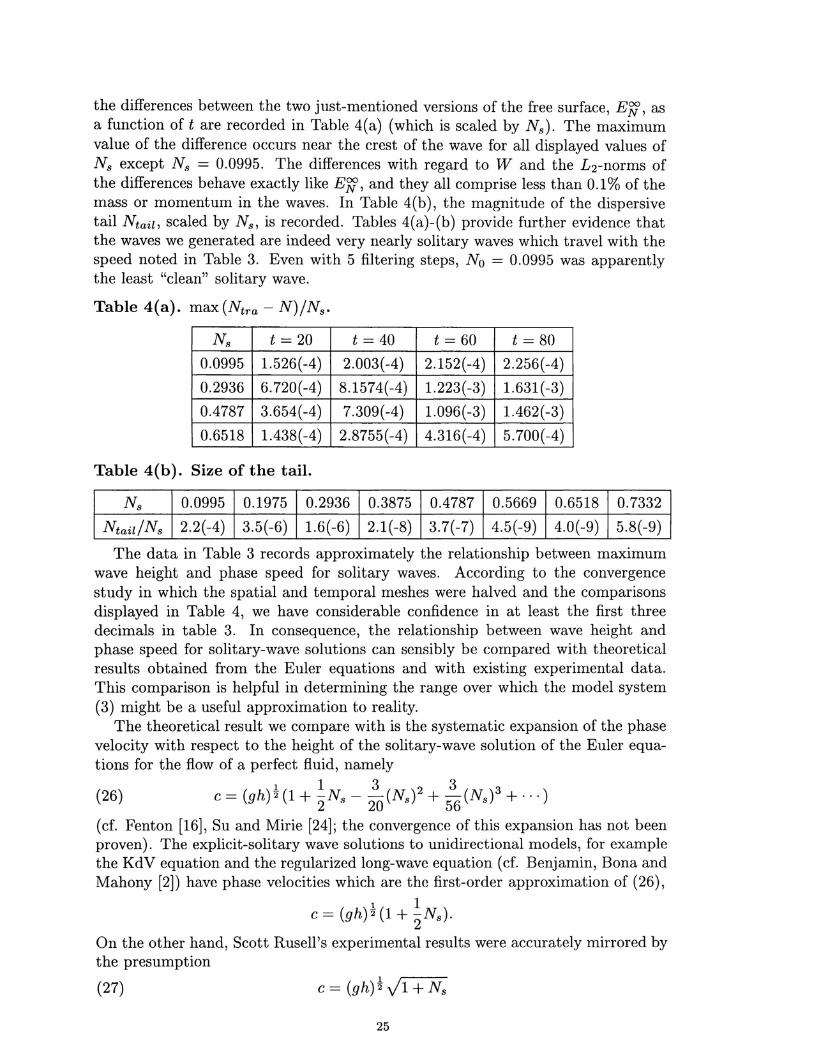
the differences between the two just-mentioned versions of the free surface, EN, asa function of t are recorded in Table 4(a) (which is scaled by Ns). The maximumvalue of the difference occurs near the crest of the wave for all displayed values ofNs except Ns = 0.0995. The differences with regard to Wand the L2-norms ofthe differences behave exactly like EN, and they all comprise less than 0.1% of themass or momentum in the waves. In Table 4(b), the magnitude of the dispersivetail Ntai1, scaled by Ns, is recorded. Tables 4(a)-(b) provide further evidence thatthe waves we generated are indeed very nearly solitary waves which travel with thespeed noted in Table 3. Even with 5 filtering steps, No = 0.0995 was apparentlythe least "clean" solitary wave.

Table 4(a). max (Ntra - N)/Ns.

Ns t = 20 t = 40 t = 60 t = 800.0995 1.526(-4) 2.003(-4) 2.152(-4) 2.256(-4)0.2936 6.720(-4) 8.1574(-4) 1.223(-3) 1.631(-3)0.4787 3.654(-4) 7.309(-4) 1.096(-3) 1.462( -3)0.6518 1.438(-4) 2.8755(-4) 4.316(-4) 5.700(-4)

Table 4(b). Size of the tail.

Ns 0.0995 0.1975 0.2936 0.3875 0.4787 0.5669 0.6518 0.7332

Ntail/Ns 2.2(-4) 3.5(-6) 1.6(-6) 2.1(-8) 3.7(-7) 4.5(-9) 4.0(-9) 5.8(-9)

The data in Table 3 records approximately the relationship between maximumwave height and phase speed for solitary waves. According to the convergencestudy in which the spatial and temporal meshes were halved and the comparisonsdisplayed in Table 4, we have considerable confidence in at least the first threedecimals in table 3. In consequence, the relationship between wave height andphase speed for solitary-wave solutions can sensibly be compared with theoreticalresults obtained from the Euler equations and with existing experimental data.This comparison is helpful in determining the range over which the model system(3) might be a useful approximation to reality.

The theoretical result we compare with is the systematic expansion of the phasevelocity with respect to the height of the solitary-wave solution of the Euler equa-tions for the flow of a perfect fluid, namely

1 1 3 2 3 3(26) c=(gh)2(1+2Ns-20(Ns) + 56 (Ns) + ... )(cf. Fenton [16], Su and Mirie [24]; the convergence of this expansion has not beenproven). The explicit-solitary wave solutions to unidirectional models, for examplethe KdV equation and the regularized long-wave equation (cf. Benjamin, Bona andMahony [2]) have phase velocities which are the first-order approximation of (26),

1 1c = (g h) 2 (1 + - N s) .

2On the other hand, Scott Rusell's experimental results were accurately mirrored bythe presumption

(27) c = (gh)~ VI + Ns

25

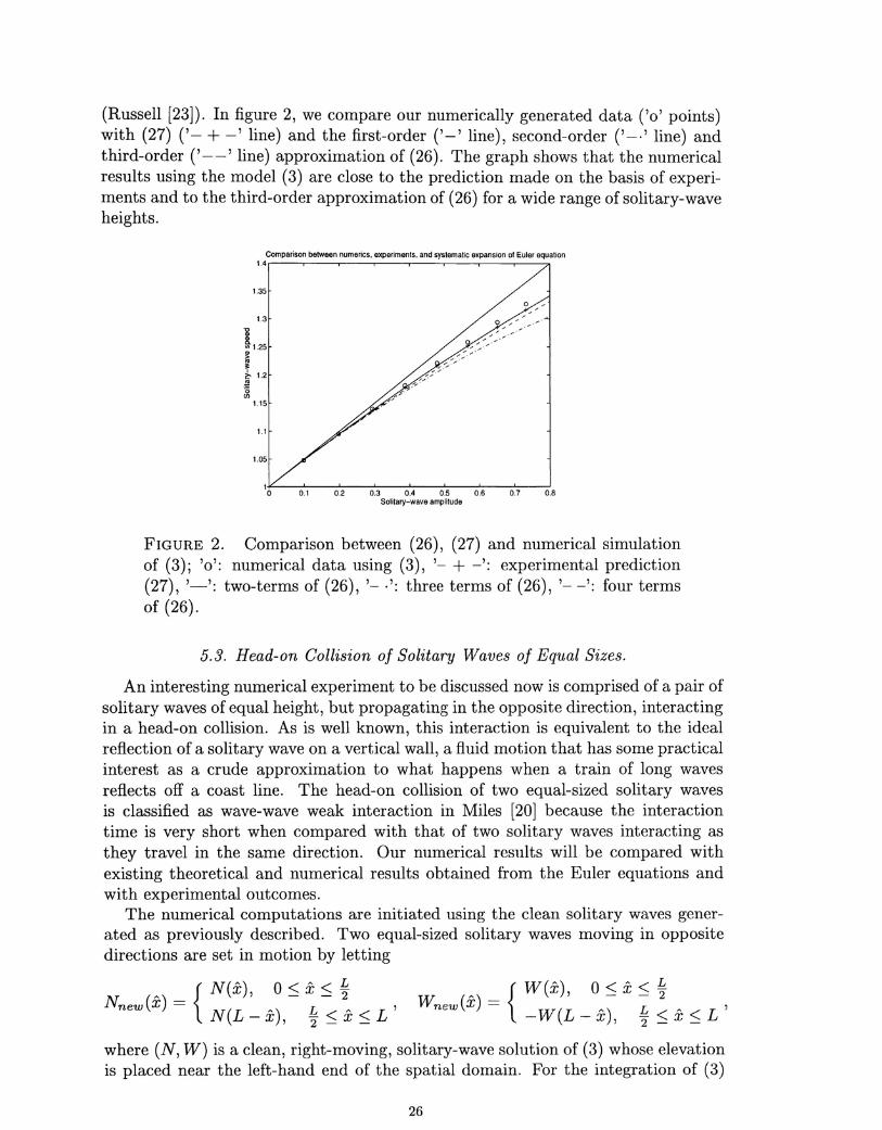
(Russell [23]). In figure 2, we compare our numerically generated data ('0' points)with (27) ('- + -' line) and the first-order ('-' line), second-order ('-.' line) andthird-order ('--' line) approximation of (26). The graph shows that the numericalresults using the model (3) are close to the prediction made on the basis of experi-ments and to the third-order approximation of (26) for a wide range of solitary-waveheights.

Comparison between numerics. experiments. and systematic expansion of Euler equation1.4

1.35

1.3

a1~g 1.25

~~b 1.2.~(5Ul

1.15

1.1

1.05

1o 0.1 0.2 0.3 0.4 0.5 0.6 0.7 0.8Solitary-wave amplitude

FIGURE 2. Comparison between (26), (27) and numerical simulationof (3); '0': numerical data using (3), '- + -': experimental prediction(27), '-': two-terms of (26), '- .': three terms of (26), '- -': four termsof (26).

5.3. Head-on Collision of Solitary Waves of Equal Sizes.

An interesting numerical experiment to be discussed now is comprised of a pair ofsolitary waves of equal height, but propagating in the opposite direction, interactingin a head-on collision. As is well known, this interaction is equivalent to the idealreflection of a solitary wave on a vertical wall, a fluid motion that has some practicalinterest as a crude approximation to what happens when a train of long wavesreflects off a coast line. The head-on collision of two equal-sized solitary wavesis classified as wave-wave weak interaction in Miles [20] because the interactiontime is very short when compared with that of two solitary waves interacting asthey travel in the same direction. Our numerical results will be compared withexisting theoretical and numerical results obtained from the Euler equations andwith experimental outcomes.

The numerical computations are initiated using the clean solitary waves gener-ated as previously described. Two equal-sized solitary waves moving in oppositedirections are set in motion by letting

A < LN(x), 0::::; x _ 2Nnew(x) = { N(L - x), ~ 50 x 50 L '

A < L

{W(X), 0::::; x _ 2

W new (x) = _W (L _ x), ~::::; X ::::;L '

where (N, W) is a clean, right-moving, solitary-wave solution of (3) whose elevationis placed near the left-hand end of the spatial domain. For the integration of (3)

26

(a) 1=0 (c) 1=51.41 (d) 1=70.300.5 0.5

0.4 1.20.4

0.3 0.310.2 02

0.1 0.10.8

0 0t==='~'-

0 50 100 150 0 50 100 1500.6

(b) 1=23.42 (e) 1=93.730.5 0.5

0.4 0.4 0.4

0.3 0.3

0.2 0.2 0.2

0.1 0.1

0 L- Or--~ °L' , '-

0 50 100 150 0 50 100 150 0 50 100 150

FIGURE 3. Time Evolution of a Head-on Collision

with this initial data, .6.x, .6.t and L are chosen as before, namely .6.x = .6.t = 0.5/32and L = 150.

Figure 3 shows a typical time evolution of the head-on collision of two equal-sizedsolitary waves with the amplitude to water depth ratio Ns = 0.4787. From (a) to(b), the solitary waves traveled for a time period i = 23.42 with essentially no changeof shape or amplitude. Part (c) shows the interaction of the two waves; notice thatthe maximum wave height at interaction is 1.0504, which is substantially more thandouble the incident wave height. Figure 3(d) is taken after the interaction whenthe two waves are moving away from each other. In (e), the two solitary waves arefurther apart and are seen to be quite similar to those in (a). A closer look at theinterval between the separating solitary waves in 3(d) and 3(e) shows that therehas been generated a secondary dispersive wave of extremely small magnitude. Asis usual for purely dispersive waves, it spreads and its amplitude diminishes withtime.

15

10

o

-5o 50 100 150

FIGURE 4. Dispersive tail.

Figure 4 and Figure 5 provide a more detailed view of the interaction. Figure 4

27

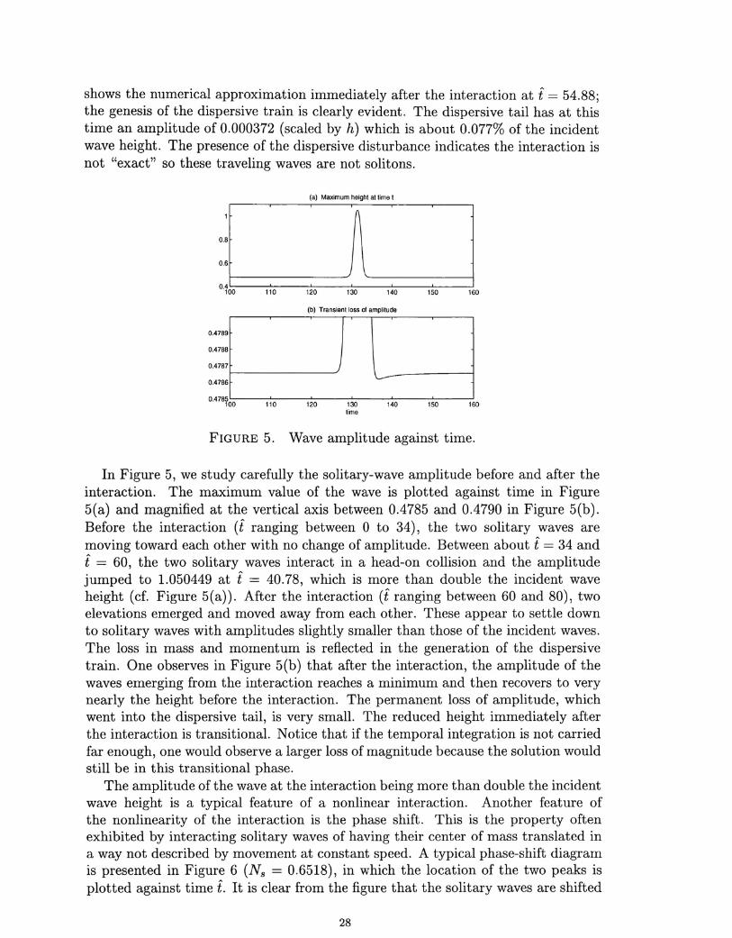
shows the numerical approximation immediately after the interaction at i = 54.88;the genesis of the dispersive train is clearly evident. The dispersive tail has at thistime an amplitude of 0.000372 (scaled by h) which is about 0.077% of the incidentwave height. The presence of the dispersive disturbance indicates the interaction isnot "exact" so these traveling waves are not solitons.

(a) Maximum height at time t-

'I ~0.8

0.6

J . ~100 110 120 130 140 150 160

(b) Transient loss of amplitude

I I , I0.4789

0.4788

0.4787

0.4786l/ L-

0.4785160100 110 120 130 140 150

time

FIGURE 5. Wave amplitude against time.

In Figure 5, we study carefully the solitary-wave amplitude before and after theinteraction. The maximum value of the wave is plotted against time in Figure5(a) and magnified at the vertical axis between 0.4785 and 0.4790 in Figure 5(b).Before the interaction (i ranging between 0 to 34), the two solitary waves aremoving toward each other with no change of amplitude. Between about i = 34 andi = 60, the two solitary waves interact in a head-on collision and the amplitudejumped to 1.050449 at i = 40.78, which is more than double the incident waveheight (cf. Figure 5(a)). After the interaction (i ranging between 60 and 80), twoelevations emerged and moved away from each other. These appear to settle downto solitary waves with amplitudes slightly smaller than those of the incident waves.The loss in mass and momentum is reflected in the generation of the dispersivetrain. One observes in Figure 5(b) that after the interaction, the amplitude of thewaves emerging from the interaction reaches a minimum and then recovers to verynearly the height before the interaction. The permanent loss of amplitude, whichwent into the dispersive tail, is very small. The reduced height immediately afterthe interaction is transitional. Notice that if the temporal integration is not carriedfar enough, one would observe a larger loss of magnitude because the solution wouldstill be in this transitional phase.

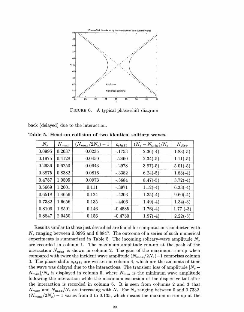
The amplitude of the wave at the interaction being more than double the incidentwave height is a typical feature of a nonlinear interaction. Another feature ofthe nonlinearity of the interaction is the phase shift. This is the property oftenexhibited by interacting solitary waves of having their center of mass translated ina way not described by movement at constant speed. A typical phase-shift diagramis presented in Figure 6 (Ns = 0.6518), in which the location of the two peaks isplotted against time i. It is clear from the figure that the solitary waves are shifted

28

50

49

48

47

46

x 45

44

43

42

41

4024 25

Phase-Shift Introduced by the Interaction of Two Solitary Waves

FIGURE 6. A typical phase-shift diagram

back (delayed) due to the interaction.

Table 5. Head-on collision of two identical solitary waves.

Ns Nmax (Nmax/2Ns) - 1 Cshift (Ns - Nmin)/Ns Ndisp0.0995 0.2037 0.0235 -.1753 2.36(-4) 1.83(-5)0.1975 0.4128 0.0450 -.2460 2.34(-5) 1.11(-5)0.2936 0.6250 0.0643 -.2978 3.97(-5) 5.01(-5)0.3875 0.8382 0.0816 -.3382 6.24(-5) 1.88(-4)0.4787 1.0505 0.0973 -.3684 8.47(-5) 3.72(-4)0.5669 1.2601 0.111 -.3971 1.12(-4) 6.33(-4)0.6518 1.4656 0.124 -.4203 1.35(-4) 9.60(-4)0.7332 1.6656 0.135 -.4406 1.49(-4) 1.34( -3)0.8109 1.8591 0.146 -0.4585 1.76(-4) 1.77 (-3)0.8847 2.0450 0.156 -0.4730 1.97( -4) 2.22( -3)

Results similar to those just described are found for computations conducted withNs ranging between 0.0995 and 0.8847. The outcome of a series of such numericalexperiments is summarized in Table 5. The incoming solitary-wave amplitude Nsare recorded in column 1. The maximum amplitude run-up at the peak of theinteraction Nmax is shown in column 2. The gain of the maximum run-up whencompared with twice the incident wave amplitude (Nmax/2Ns)-1 comprises column3. The phase shifts Cshift are written in column 4, which are the amounts of timethe wave was delayed due to the interactions. The transient loss of amplitude INs-

Nminl/Ns is displayed in column 5, where Nmin is the minimum wave amplitudefollowing the interaction while the maximum excursion of the dispersive tail afterthe interaction is recorded in column 6. It is seen from columns 2 and 3 thatNmax and Nmax/Ns are increasing with Ns. For Ns ranging between 0 and 0.7332,(Nmax/2Ns) - 1 varies from 0 to 0.135, which means the maximum run-up at the

29

middle is between 0 to 13.5% more than double the incident wave height. Thedata is consistent with the proposition that (Nmax/2Ns) - 1 -+ 0 as Ns -+ 0, sogoing over to the linear theory in the limit of infinitesimal amplitude. The phaseshift in column 4 also increases as Ns increases and likewise points to the propertyCshift -+ 0 when Ns -+ O. Column 5 confirms that for this model system, there isa transitional loss of magnitude, which is small when compared with the existingexperimental results. It is noticed during the computation that the magnitude ofthis transitional loss and the height of the dispersive tail (column 6) are sensitive tothe cleanness of the incoming solitary wave. One observes much larger secondaryexcursions due to the tails of the incoming disturbance when the initial configurationis not quite close to a true solitary wave. If we use one, instead of four, filteringstep for No = 0.2, and then interact the resulting approximate solitary wave withitself in a head-on collision, the entries corresponding to row 2 in Table 5 are asfollows.

Ns Nmax (Nmax/2Ns) - 1 Cshift (Ns - Nmin)/Ns Ndisp

0.1975 0.4128 0.0450 -.2460 1.7(-3) 5.8(-4)

Thus the noisier approximation generates considerably larger values of the transi-tionalloss of magnitude and the maximum excursion of the dispersive tail.

The relative magnitude of this transitional loss of amplitude and the height ofthe dispersive wave both increase as Ns increases. (The values associated withNs = 0.0995 may not be accurate because the incident solitary waves are notespecially clean.) In our computations, we did not observe large permanent lossof amplitude. The solitary waves appear to always recover from their transitionalloss and return to very nearly their original height. These observations are atodds with the experimental results of Renouard, Santos and Temperville [22]. Thediscrepancy between experimental outcomes and our numerical simulations owes toat least two major aspects. First, dissipative effects are always substantial in wavetanks on laboratory scales. Second, it is quite difficult to generate a truly cleansolitary wave in a laboratory setting. As just indicated, numerical simulations withless accurate approximations to solitary waves led to significant permanent loss ofamplitude due to interaction, just as observed in the laboratory.

A quantitative comparison is now undertaken between numerical data in Table5 and existing theoretical and numerical results obtained via the Euler equations,and with existing experimental results. We first compare the maximum heightof the wave during interaction and the phase shift after the collision. Since thecollision of equal-sized solitary waves is equivalent to the reflection of a solitary waveagainst a vertical wall in the absence of viscous effects, comparisons of the numericalsimulations reported above can be made with theoretical and other results for thislatter problem. From the Euler equations, one obtains a systematic expansion ofthe maximum wave amplitude Nmax along the wall in terms of Ns, which is (cf.Byatt-Smith [9], Oikawa and Yajima [21] and Su and Mirie [24])

(28) 1 2 3( 3Nmax = 2Ns + -(Ns) + - Ns) + ...2 4

30

and similarly for the phase-shift Cshift

(29)

(the convergence of these series is again an open question).

Maximum Run-up at the cenler

linear: --Su, second-order: solid lineOur numerical: 0

1.8

1.6

1.4

1.2

0.8

0.6

0.3 0.4 0.5 0.6 0.7 0.8 0.9aJh

FIGURE 7. Maximum run-up, interaction of two equal solitary waves;'0': Numerical simulation using (7), '- -': one term of (28), '-": twoterms of (28).

In Figure 7, the maximum wave height at the center of the interaction is com-pared with both the first- and second-order approximations in (28). The numericalsimulations agree with the second-order approximation more closely for a widerange of incident wave heights. The third-order approximation is more accurateonly when Ns is sufficiently small.

Phase-Shift

0.5

0.4

.cCi 0.3

0.2

Approx Theory: -+-

Numerical: -0-

o Ql Q2 Q3 0.4 M Q6 Q7 Q8 Q9aJh

FIGURE 8. Phase-shift.

31

The phase-shift introduced by the interaction of the two solitary waves is shownin Figure 8 along with the associated graph of the leading-order approximation (29)to the phase-shift according to the Euler equations. The numerically generatedvalues lie close to, but below those predicted by (29). One possible reason for theslight discrepancy is that we did not wait long enough in our computations for theoutgoing waves to recover, and a small error in the phase speed could result in arelatively large error in Cshift.

Overall, our numerically generated data shows the system (3) models solitary-wave propagation and interaction nicely even when the amplitude of the wave isnot especially small. Indeed, our numerical computations can handle amplitudesNs as high as 7, which is of course not relevant to practical situations.

Comparison is now made between the numerical data and existing experimentalresults found in Camfield and Street [11] , Maxworthy [19], and in particular withmore recent results obtained in Renouard, Santos and Temperville [22]. Regardingthe reflexion of a solitary wave from a plane vertical wall, the maximum run-upson the wall in all the experiments agree pretty well with (28) and the phase shiftsreported in [22] agree with (29) qualitatively and to some extent quantitatively.Reasons for the lack of detailed agreement with experiments certainly include theviscous effects in the boundary layer along the channel walls, which is not modeledhere. Indeed, the comparisons of experimental data taken in a fluid with the pre-dictions of a unidirectional model related to (3) in [4] shows clearly that detailedagreement at least for laboratory scales depends on accurate modeling of dissipativeeffects. In addition, the solitary waves generated in the laboratory are not clean, sothe incident wave is not clean and the reflected wave encounters a dispersive tail asit comes off the wall. This aspect also was essentially absent in the numerical simu-lations. In [22], they also reported the transitional loss of magnitude and dispersivetails after the interaction, but with much larger magnitude than observed in ournumerical computations. They found that (Ns - Nout)/Ns and Ndisp depend onNs at third order. The magnitude of either the loss of amplitude or the dispersivetail is about 10% of the incident amplitude when Ns is about 0.6. We suspect thatsome of this might come from the effect of the dispersive tails following the incidentwaves. Because of the nature of our model system, which is only formally first ordercorrect with respect to the small parameter E, we are not in a position to say if thechange of amplitude is fifth-order in E (see Byatt-Smith [10]) or third-order in E (seeSu and Mirie [24]). We are currently working on higher-order Boussinesq systemsfor two-way propagation of water waves [14] and expect in due course to betterunderstand these phenomena. We are also preparing our own experiments in whichwe will observe directly the collision of solitary waves rather than as modeled byinteraction with a vertical wall.

Numerical experiments of head-on collisions have been reported in various pa-pers. A modified Marker and Cell technique (SUMMAC) was used on the fullEuler equations in Chan and Street [12] and Tang, Patel and Landweber [25],while Fourier methods were used in Fenton and Rienecker [17] on the Euler equa-tions. In Su and Mirie [24], the authors computed solutions using a Boussinesq-likesystem. Qualitatively, (28) and (29) agreed with all the numerical results. Themajor difference is the existence and the magnitude of permanent loss (the heightsof the outgoing solitary waves are lower than that of the associated incoming soli-

32

tary waves), the transitional loss and the dispersive tail. We concluded from ournumerical results that there is a dispersive tail and a transitional loss of magni-tude associated with the interaction, but the incoming and outgoing solitary waveseventually have essentially the same height, the difference being less than 10-6, avalue which could not be observed in experiments.

5.4. Head-on Collision of Waves with Different Heights.

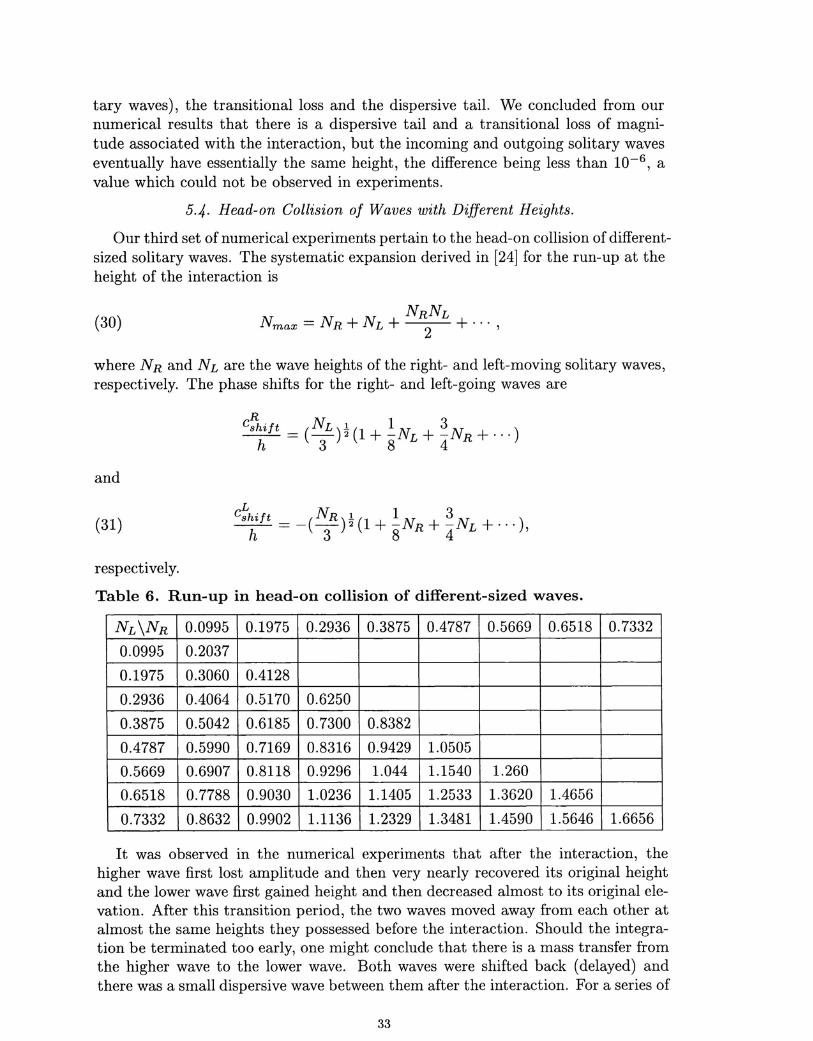
Our third set of numerical experiments pertain to the head-on collision of different-sized solitary waves. The systematic expansion derived in [24] for the run-up at theheight of the interaction is

(30)

where NR and NL are the wave heights of the right- and left-moving solitary waves,respectively. The phase shifts for the right- and left-going waves are

and

(31)

respectively.

Table 6. Run-up in head-on collision of different-sized waves.

NL\NR 0.0995 0.1975 0.2936 0.3875 0.4787 0.5669 0.6518 0.7332

0.0995 0.2037

0.1975 0.3060 0.4128

0.2936 0.4064 0.5170 0.6250

0.3875 0.5042 0.6185 0.7300 0.8382

0.4787 0.5990 0.7169 0.8316 0.9429 1.05050.5669 0.6907 0.8118 0.9296 1.044 1.1540 1.260

0.6518 0.7788 0.9030 1.0236 1.1405 1.2533 1.3620 1.4656

0.7332 0.8632 0.9902 1.1136 1.2329 1.3481 1.4590 1.5646 1.6656

It was observed in the numerical experiments that after the interaction, thehigher wave first lost amplitude and then very nearly recovered its original heightand the lower wave first gained height and then decreased almost to its original ele-vation. After this transition period, the two waves moved away from each other atalmost the same heights they possessed before the interaction. Should the integra-tion be terminated too early, one might conclude that there is a mass transfer fromthe higher wave to the lower wave. Both waves were shifted back (delayed) andthere was a small dispersive wave between them after the interaction. For a series of

33

wave heights of the right- and left-moving waves, we computed the maximum waveamplitudes at the interaction. These are listed in Table 6, while the phase-shiftsfor the left-going waves are listed in Table 7. The phase-shifts of the right-goingwaves can be found by switching the positions of the left- and right-going waves.

Table 7. Phase-shifts of the left-going wave.

NL\NR 0.0995 0.1975 0.2936 0.3875 0.4787 0.5669 0.6518 0.73320.0995 .1753 .2538 .3120 .3570 .3960 .4318 .4595 .49250.1975 .1782 .2460 .3024 .3531 .3854 .4246 .4546 .47410.2936 .1782 .2436 .2978 .3403 .3809 .4145 .4439 .46940.3875 .1714 .2400 .2943 .3382 .3738 .4066 .4399 .46410.4787 .1655 .2366 .2893 .3337 .3684 .4001 .4323 .45610.5669 .1627 .2315 .2849 .3285 .3637 .3971 .4234 .45270.6518 .1648 .2248 .2819 .3226 .3597 .3942 .4203 .44260.7332 .1590 .2288 .2800 .3183 .3589 .3873 .4151 .4406

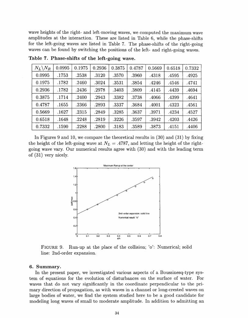
In Figures 9 and 10, we compare the theoretical results in (30) and (31) by fixingthe height of the left-going wave at NL = .4787, and letting the height of the right-going wave vary. Our numerical results agree with (30) and with the leading termof (31) very nicely.

Maximum Runup at the center1.6

1.4o

1.2

~.§.0.8.c~

0.6

0.4

0.2

2nd-order expansion: solid line

Numerical result "0"

0.1 0.2 0.3 0.4 0.5 0.6 0.7 0.8aJh

FIGURE 9. Run-up at the place of the collision; '0': Numerical; solidline: 2nd-order expansion.

6. Summary.In the present paper, we investigated various aspects of a Boussinesq-type sys-

tem of equations for the evolution of disturbances on the surface of water. Forwaves that do not vary significantly in the coordinate perpendicular to the pri-mary direction of propagation, as with waves in a channel or long-crested waves onlarge bodies of water, we find the system studied here to be a good candidate formodeling long waves of small to moderate amplitude. In addition to admitting an

34

Phase-Shill of Lell-going Wave

0.5

0.4

oo 0.1

oo

o

Leading tann in the exapnslon: solid line

Numerical: "0"

~ ~ M M M ~ MHeight 01RighI-going Wave

FIGURE 10. Phase-shift

appropriate theory of well-posedness for suitable initial-boundary-value problems,it is straightforward to construct accurate, efficient numerical schemes for the ap-proximation of the system's solutions. We suggested a numerical scheme which isfourth-order accurate in both its spatial and its temporal approximation, which isunconditionally stable and which features good accuracy for work expended. Thescheme is based on a pair of integral equations equivalent to the system of differ-ential equations that comprise the Boussinesq system. Because of this formulation,it is comparatively easy to impose boundary conditions without disturbing eitherthe order of accuracy or the convergence and stability properties.

Our study featured also preliminary comparisons of the model's predictions madevia a computer code constructed on the basis of the numerical scheme analyzed inSection 3, with theoretical results derived from the Euler equations and with exper-imental results. In the numerical experiments connected with the head-on collisionof solitary waves, we find our results to correspond well with facts about such in-teractions derived from the full Euler equations. There are quantitative differencesbetween what is predicted on the basis of our model and experimental results,however. Earlier work based on unidirectional models for water-wave propagationindicate it likely that the absence of an accurate rendering of dissipative effectsaccounts for a good deal of the discrepancy.

A further study is planned along the lines set forth in [4] for unidirectionalpropagation, in which dissipation is incorporated and detailed comparisons aremade with dynamically recorded wave data.

Acknowledgments. This work was supported in part by NSF grants DMS-9205300and DMS-9410188 and by a Keck Foundation grant. JLB gratefully acknowledgesCNRS support at the Centre de Mathematiques et de Leurs Applications, EcoleNormal Superieure de Cachan.

35

References

[1] C. J. Amick & J. F. Toland, "On solitary waves of finite amplitude," Arch.Rational Mech. Anal. 76 (1981), 9-95.

[2] T. B. Benjamin, J. L. Bona & J. J. Mahony, "Model equations for long wavesin nonlinear dispersive systems," Phil. Trans. Royal Soc. London. A 272 (1972),47-78.

[3] J. L. Bona & V. A. Dougalis, "An initial- and boundary-value problem for amodel equation for propagation of long waves," Journal of Mathematical Anal-ysis and Applications 75 (1980), 503-522.

[4] J. L. Bona, W. G. Pritchard & L. R. Scott, "An evaluation of a model equationfor water waves," Phil. Trans. R. Soc. London. A 302 (1981), 457-510.

[5] J. L. Bona, W. G. Pritchard & L. R. Scott, "Numerical schemes for a model fornonlinear dispersive waves," J. Compo Physics 60 (1985), 167-186.

[6] J. L. Bona, J.-C. Saut & J. F. Toland, "Boussinesq equations and other systemsfor small-amplitude long waves in nonlinear dispersive media," preprint (1996).

[7] J. L. Bona & R. Smith, "A model for the two-way propagation of water wavesin a channel," Math. Proc. Cambridge Phil. Soc. 79 (1976), 167-182.

[8] J. Boussinesq, "Theorie de l'intumescence liquide appelee onde solitaire ou detranslation se propageant dans un canal rectangulaire," Comptes Rendus del'Acadmie de Sciences 72 (1871), 755-759.

[9] J. G. B. Byatt-Smith, "An integral equation for unsteady surface waves and acomment on the Boussinesq equation," J. Fluid Mech. 49 (1971),625-633.

[10] J. G. B. Byatt-Smith, "The reflection of a solitary wave by a vertical wall," J.Fluid Mech. 197 (1988), 503-521.

[11] F. E. Camfield & R. L. Street, "Shoaling of solitary waves of small amplitude,"A.S.C.E. J., Waterways and Harbors Division 95 (1969), 1-22.

[12] R. K.-C. Chan & R. L. Street, "A computer study of finite-amplitude waterwaves," Journal of Computational Physics 6 (1970), 68-94.

[13] M. Chen, "Explicit solitary-wave solutions of model systems describing two-waypropagation of water waves," In preparation (1996).

[14] M. Chen & J. L. Bona, "Study of higher-order Boussinesq systems for waterwaves," preprint (1995).

[15] P. Davis & P. Rabinowitz, Methods of numerical integration, Academic Press,New York, 1984.

[16] J. D. Fenton, "A ninth-order solution for the solitary wave," J. Fluid Mech. 53(1972), 257-271.

[17] J. D. Fenton & M. M. Rienecker, "A Fourier method for solving non-linearwater-wave problems:," J. Fluid Mech.118 (1982),411-443.

[18] E. Isaacson & H. B. Keller, Analysis of numerical methods, Wiley, New York,1966.

[19] T. Maxworthy, "Experiments on collision between solitary waves," J. FluidMech. 76 (1976), 177-185.

36

[20] J. W. Miles, "Obliquely interacting solitary waves," J. Fluid Mech. 79 (1977),157-159.

[21] M. Oikawa & N. Yajima, "Interaction of solitary waves; a perturbation approachto non-linear systems," J. Phys. Soc. Japan. 34 (1973), 1093-1099.

[22] D. P. Renouard, F. J. Seabra Santos & A. M. Temperville, "Experimental studyof the generation, damping, and reflexion of a solitary wave," Dynamics of At-mospheres and Oceans 9 (1985),341-358.

[23] J. Scott Russell, "Report on waves," Rept. Fourteenth Meeting of the BritishAssociation for the Advancement of Science (1844).

[24] C. H. Su & R. M. Mirie, "On head-on collisions between two solitary waves," J.Fluid Mech. 98 (1980), 509-525.

[25] C. J. Tang, V. C. Patel & 1. Landweber, "Viscous effects on propagation andreflection of solitary waves in shallow channels," J. Comput. Phys. 88 (1990),86-113.

[26] G. B. Whitham, Linear and nonlinear waves, J. Wiley, New York, 1974.

37