a brief introduction to econometrics in stan - github pages · these notes are for a one-day short...

A brief introduction to econometrics in StanJames Savage

2017-04-30

Contents

About 5The structure . . . . . . . . . . . . . . . . . . . . . . . . . . . . . . . . . . . . . . . . . . . . . . . . 6

1 Modern Statistical Workflow 71.1 Modern Statistical Workflow . . . . . . . . . . . . . . . . . . . . . . . . . . . . . . . . . . . . 71.2 Tools of the trade: borrowing from software engineering . . . . . . . . . . . . . . . . . . . . . 19

2 An introduction to hierarchical modeling 21

3 Some fun time series models 293.1 This session . . . . . . . . . . . . . . . . . . . . . . . . . . . . . . . . . . . . . . . . . . . . . . 293.2 A state space model involving polls . . . . . . . . . . . . . . . . . . . . . . . . . . . . . . . . . 33

3

4 CONTENTS

About

These notes are for a one-day short course in econometrics using Stan. The main reason to learn Stan is to fitmodels that are difficult to fit using other software. Such models might include models with high-dimensionalrandom effects (about which we want to draw inference), models with complex or multi-stage likelihoods,or models with latent data structures. A second reason to learn Stan is that you want to conduct Bayesiananalysis on workhorse models; perhaps you have good prior information, or are attracted to the possibilityof making probabilistic statements about predictions and parameter estimates.

While this second reason is worthwhile, it is not the aim of this course. This course introduces a fewworkhorse models in order to give you the skills to build richer models that extract the most informationfrom your data. There are three sessions:

1. An introduction to Modern Statistical Workflow, using an instrumental variables model as the example.We will also touch on Simultaneous Equations Modeling.

2. Hierarchical models and hierarchical priors, of which we can consider panel data a special case. We’llcover fixed and random effects, post-stratification, and the Gelman-Bafumi correction.

3. An introduction to time-series models, including time-varying parameters, latent factor models, andstructural VARs.

These notes have a few idiosyncracies:

Tricks and shortcuts will look like this

The code examples live in the models/ folder of the book’s repository, (https://github.com/khakieconomics/shortcourse/models).

We use two computing languages in these notes. The first is Stan, a powerful modeling language thatallows us to express and estimate probabilistic models with continuous parameter spaces. Stan programsare prefaced with their location in the models/ folder, like so:

// models/model_1.stan// ... model code here

We also use the R language, for data preparation, calling Stan models, and visualising model results. Rprograms live in the scripts/ folder; they typically read data from the data/ folder, and liberally usemagrittr syntax with dplyr. If this syntax is unfamiliar to you, it is worth taking a look at the excellentvignette to the dplyr package. Like the Stan models, all R code in the book is prefaced with its location inthe book’s directory.# scripts/intro.R# ... data work here

It is not necessary to be an R aficionado to make the most of these notes. Stan programs can be calledfrom within Stata, Matlab, Mathematica, Julia and Python. If you are more comfortable using thoselanguages than R for data preparation work, then you should be able to implement all the models in thisbook using those interfaces. Further documentation on calling Stan from other environments is available athttp://mc-stan.org/interfaces/.

While Stan can be called quite easily from these other programming environments, the R implementation

5

https://github.com/khakieconomics/shortcourse/models

https://github.com/khakieconomics/shortcourse/models

https://cran.rstudio.com/web/packages/dplyr/vignettes/introduction.html

https://cran.rstudio.com/web/packages/dplyr/vignettes/introduction.html

http://mc-stan.org/interfaces/

6 CONTENTS

is more fully-fleshed—especially for model checking and post-processing. For this reason we use the Rimplementation of Stan, rstan in this book.

The structure

An important premise in these is that we should only build richer, more complex models when simple oneswill not do. After explaining the necessary preliminary concepts, Each session is set up around this theme.The first session offers an introduction to Stan, walking you through the steps of building, estimating, andchecking a probability model. We call this procedure Modern Statistical Workflow, and recommend it befollowed for essentially all modeling tasks. If you’re an experienced modeler and understand the preliminariesalready, this is a good place to start.The second session covers hierarchical modeling. The central notion in hierarchical modeling is that our datahas some hierarchy. Some examples might illustrate the idea:

• Our observations are noisy measures of some true value, about which we want to infer.• We have multiple observations from many administrative units, for example students within a school

within a region.• We observe many individuals over time (panel data).

There is a large cultural difference between panel/hierarchical data as used by econometricians and as usedby Bayesian statisticians. We’ll take a more statistical approach in this book. The big difference is thatBayesian statisticians think that the primary goal of using hierarchical data is to fit a model at the level ofthe individual, but recognising that information from other individuals might be useful in estimating thatmodel. It’s a crass simplification, but economists tend to view the goal of using panel data as helping toestimate an unbiased or less biased treatment effect that abstracts from unobserved information fixed withinthe individual. These are different goals, and we will discuss them later.We will cover fixed and random effects, and the Gelman-Bafumi correction (which makes random effectsmodels more widely applicable). We also discuss how to incorporate instruments in these models.The last session introduces some fun time-series models. Chapter seven illustrates how to implement moreadvanced multivariate time-series models. These include Structural Vector Autoregressions (SVAR), factormodels, and state-space methods, including time-varying parameter regressions, and low-to-high frequencymissing values interpolation.

0.0.1 A note on data

Through this short course, we will not use any real data, but rather force you to simulate fake data wherethe “unknowns are known”. This is very good practice, both from the perspective of model checking, butalso helping you to understand the underlying data generating process that you are trying to model.

Chapter 1

Modern Statistical Workflow

This session introduces the process I recommend for model building, which I call “Modern Statistical Work-flow”.

1.1 Modern Statistical Workflow

The workflow described here is a template for all the models that will be discussed during the course. Ifyou work by it, you will learn models more thoroughly, spot errors more swiftly, and build a much betterunderstanding of economics and statistics than you would under a less rigorous workflow.The workflow is iterative. Typically we start with the simplest possible model, working through each stepin the process. Only once we have done each step do we add richness to the model. Building models up likethis in an iterative way will mean that you always have a working version of a model to fall back on. Theprocess is:

1. Write out a full probability model. This involves specifying the joint distribution for your parame-ters/latent variables and the conditional distribution for the outcome data.

2. Simulate some data from the model with assumed values for the parameters (these might be quitedifferent from the “true” parameter values).

3. Estimate the model using the simulated data. Check that your model can recover the known parametersused to simulate the data.

4. Estimate the model parameters conditioned on real data.5. Check that the estimation has run properly.6. Run posterior predictive checking/time series cross validation to evaluate model fit.7. Perform predictive inference.

Iterate the entire process to improve the model! Compare models—which model are the observed outcomesmore plausibly drawn from?

1.1.1 Example: A model of wages

Before building any model, it is always worth writing down the questions that we might want to ask. Some-times, the questions will be relativey simple, like “what is the difference in average wages between menand women?” Yet for most large-scale modeling tasks we want to build models capable of answering manyquestions. In the case of wages, they may be questions like:

• If I know someone is male and lives in the South what should I expect their wages to be, holding otherpersonal characteristics constant?

• How much does education affect wages?

7

8 CHAPTER 1. MODERN STATISTICAL WORKFLOW

• Workers with more work experience tend to earn higher wages. How does this effect vary acrossdemographic groups?

• Does variance in wages differ across demographic groups?

As a good rule of thumb, the more questions you want a model to be able to answer, the more complex themodel will have to be. The first question above might be answered with a simple linear regression model, thesecond, a more elaborate model that allows the relationship between experience and wages to vary acrossdemographic groups; the final question might involve modeling the variance of the wage distribution, notjust its mean.

The example given below introduces a simple linear model of wages given demographic characteristics, withthe intent of introducing instrumental variables—the first trick up our sleeve for the day. We’ll introducetwo competing instrumental variables models: the first assuming independence between the first and secondstage regressions and the second modeling them jointly.

Let’s walk through each step of the workflow, gradually introducing Stan along the way. While we’re notgoing to estimate the model on real data, we want to make sure that the model we build is sane. As such we’lllook at the characteristics of wages for some real data. This data comes from some wage and demographicsdata from the 1988 Current Population Survey, which comes in R’s AER package. This dataset contains theweekly wage for around 28,000 working men in 1988; prices are in 1992 dollars. You can load the datasetinto your R workspace like so:library(AER)data("CPS1988")

1.1.2 Step 1: Writing out the probability model

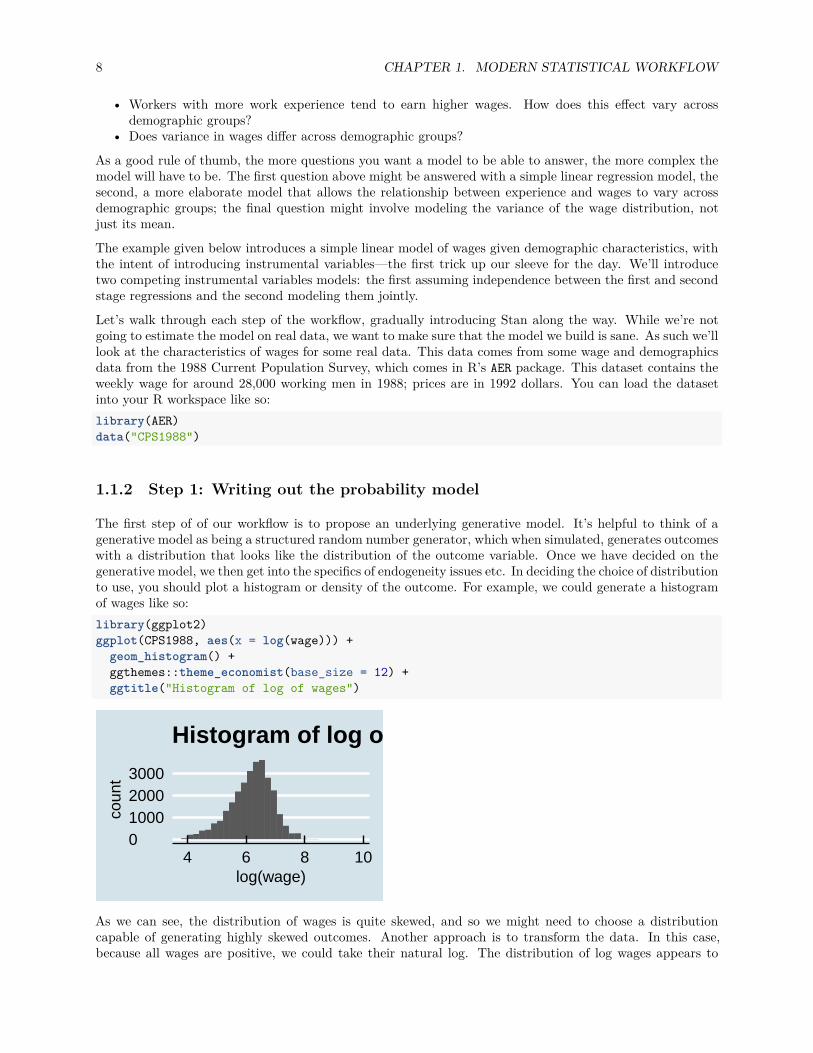
The first step of of our workflow is to propose an underlying generative model. It’s helpful to think of agenerative model as being a structured random number generator, which when simulated, generates outcomeswith a distribution that looks like the distribution of the outcome variable. Once we have decided on thegenerative model, we then get into the specifics of endogeneity issues etc. In deciding the choice of distributionto use, you should plot a histogram or density of the outcome. For example, we could generate a histogramof wages like so:library(ggplot2)ggplot(CPS1988, aes(x = log(wage))) +

geom_histogram() +ggthemes::theme_economist(base_size = 12) +ggtitle("Histogram of log of wages")

0100020003000

4 6 8 10log(wage)

coun

t

Histogram of log of wages

As we can see, the distribution of wages is quite skewed, and so we might need to choose a distributioncapable of generating highly skewed outcomes. Another approach is to transform the data. In this case,because all wages are positive, we could take their natural log. The distribution of log wages appears to

1.1. MODERN STATISTICAL WORKFLOW 9

be far more normal than the initial distribution, and it possible that the non-normality is explainable usingdemographic characteristics.ggplot(CPS1988, aes(x = log(wage))) +

geom_histogram() +ggthemes::theme_economist(base_size = 12) +ggtitle("Histogram of log of wages")

0100020003000

4 6 8 10log(wage)

coun

t

Histogram of log of wages

If we decide to choose a normal density as the data-generating process, and assume that the conditionaldistribution of one person’s wage does not depend on the conditional distribution of another person’s, wecan write it out like so:

log(wage)i ∼ Normal(µi, σi)

which says that a person i’s wage is distributed according to a normal distribution with location µi and scaleσi. In the case of a normal density, the location is the mean, and the scale is the standard deviation. Weprefer to use “location” and “scale” rather than “mean” and “standard deviation” because the terminologycan carry across to other densities whose location and scale parameters don’t correspond to the mean orstandard deviation.

Let’s be clear about what this means. This generative model says that each individual’s (log) wage is notcompletely determined—it involves some amount of luck. So while on average it will be µi, luck will resultin differences from this average, and these differences have a standard deviation of σi.

Notice that both parameters µi and σi vary across each individual. One of the main challenges of building agood model is to come up with functional forms for µi and σi, taking into account the information availableto us. For instance, the (normal) linear regression model uses a (row) vector of individual characteristicsXi = (educationi, experiencei, . . . ), along with a set of parameters that are common to all individuals (anintercept α, coefficients β and a scale parameter σ). The generative model is then:

log(wage)i ∼ Normal(α + Xiβ, σ)

which is the same as saying:

log(wage)i = α + Xiβ + ϵi with ϵi ∼ N(0, σ)

Note that we’ve made “modeling assumptions” µi = α + Xiβ and σi = σ. The parameters of the generativemodel are both “true” and unknown. The entire point is to peform inference in order to get probabilisticestimates of the “true” parameters.


1.1.2.1 Choosing the right generative model

Above, we picked out a normal density for log wages (which corresponds to a lognormal density for wages) asa reasonable first step in modeling our wage series. How did we get to this choice? The choice of distributionto use should depend on the nature of your outcome variables. Two good rules of thumb are:

1. The chosen distribution should not give positive probability to impossible outcomes. For example,wages can’t be negative, and so if we were to use a normal density (which gives positive probability toall outcomes) to model wages, we would be committing an error. If an outcome is outcome is binaryor count data, the model should not give weight to non-integer outcomes. And so on.

2. The chosen distribution should give positive weight to plausible outcomes.

1.1.2.2 Choosing priors

To complete our probability model, we need to specify priors for the parameters β and σ. Again, these priorsshould place positive probabilistic weight over values of the parameters that we consider possible, and zeroweight on impossible values (like a negative scale σ). In this case, it is common to assume normal priors forregression coefficients and half-Cauchy or half-Student-t priors on scales.A great discussion of choosing priors is available here.

1.1.2.3 Thinking ahead: are our data endogenous? Instrumental variables

As you will see in the generative model above, ϵ are as though they’ve been drawn from a (normal) randomnumber generator, and have no systematic relationship to the variables in X. Now what is the economicmeaning of ϵ? The way I prefer to think about it is as a catch-all containing the unobserved informationthat is relevant to the outcome.We need to think ahead: is there unobserved information that will be systematically correlated with X? Canwe tell a story that there are things that cause both some change in one of our X variables and also ourobserved wages? If such information exists, then at the model estimation stage we will have an unobservedconfounder problem, and we need to consider it in our probability model. A common way of achiving this isto use instrumental variables.An instrumental variable is one that introduces plausible exogenous variation into our endogenous regressor.For example, if we have years of education on the right hand side, we might be concerned that the same sortsof unobserved factors—family and peer pressure, IQ etc.—that lead to high levels of education might alsolead to high wages (even in absense of high levels of education). In this case we would want to “instrument”education, ideally with an experimental treatment that randomly assigned some people to higher rates ofeducation and others to less. In reality, such an experiment might not be possible to run, but we might find“natural experiments” that result in the same variation. The most famous case of such an instrument is theVietnam war draft (Angrist and Kreuger, 1992).There are a few ways of incorporating instrumental variables. The first is so-called “two stage least squares”in which we first regress the endogenous regressor on the exogenous regressors (Xedu,i) plus an instrumentor instruments Zi. In the second stage we replace the actual values of education with the fitted values fromthe first stage.Stage one:

educationi ∼ Normal(αs1 + X−edu,iγ + Ziδ, σs1)

Stage two:

log(wagei) ∼ Normal(αs2 + X−edu,iβ + (αs1 + X−edu,iγ + Ziδ)τ, σs2)

(In the second stage, we only estimate αs2, β, τ and σs2; the other parameters’ values are from the first stage).


If we treat the uncertainty of the first model approproately in the second (as is automatic in Bayes), thentwo stage least squares yields an consistent estimate of the treatment effect τ (that is, as the number ofobservations grows, we get less bias). But it may be inefficient in the case when the residuals of the datagenerating processes in stage one and stage two are correlated.The second method of implementing instrumental variables is as a simultaneous equations model. Underthis framework, the generative model is

(log(wagei), edui)′ ∼ Multi normal ((µ1,i, µ2,i)′, Σ)

where

µ1,i = αs2 + X−edu,iβ + (αs1 + X−edu,iγ + Ziδ)τ

andµ2,i = αs1 + X−edu,iγ + Ziδ

You will see: this is the same as the two stage least squares model above, exept we have allowed the errors tobe correlated across equations (this information is in the covariance matrix Σ). Nobody really understandsraw numbers from Covariance matrices, so we typically decompose covariance into the more interpretablescale vector σ and correlation matrix Ω such that Σ = diag(σ)Ωdiag(σ). This decomposition also allows usto use more interpretable priors.We now have two possible models. What we’ll do below is simulate data from the second model with knownparmaters. Then we’ll code up both models and estimate each, allowing us to perform model comparison.

1.1.3 Step 2: Simulating the model with known parameters

We have now specified two probability models. What we will do next is simulate some data from thesecond (more complex model), and then check to see if we can recover the (known) model parameters byestimating both the correctly specified and incorrectly specified models above. Simulating and recoveringknown parameters is an important checking procedure in model building; it often helps catch errors in themodel and clarifies the model in the mind of the modeler.Now that we have written out the data generating model, let’s generate some known parameters and covari-ates and simulate the model. First: generate some values for the data and paramaters.# Generate a matrix of random numbers, and values for beta, nu and sigma

set.seed(48) # Set the random number generator seed so that we get the same parametersN <- 500 # Number of observationsP <- 5 # Number of covariatesX <- matrix(rnorm(N*P), N, P) # generate an N*P covariate matrix of random dataZ <- rnorm(N) # an instrument

# The parameters governing the residualssigma <- c(1, 2)Omega <- matrix(c(1, .5, .5, 1), 2, 2)

# Generate some residualsresid <- MASS::mvrnorm(N, mu = c(0, 0), Sigma = diag(sigma)%*% Omega %*% diag(sigma))

# Now the parameters of our modelbeta <- rnorm(P)tau <- 1 # This is the treatment effect we're looking to recoveralpha_1 <- rnorm(1)


alpha_2 <- rnorm(1)gamma <- rnorm(P)delta <- rnorm(1)

mu_2 <- alpha_1 + X%*%gamma + Z*deltamu_1 <- alpha_2 + X%*%beta + mu_2*tau

Y <- as.numeric(mu_1 + resid[,1])endog_regressor <- as.numeric(mu_2 + resid[,2])

# And let's check we can't recapture with simple OLS:

lm(Y ~ . + endog_regressor, data = as.data.frame(X))

1.1.4 Writing out the Stan model to recover known parameters

A Stan model is comprised of code blocks. Each block is a place for a certain task. The bold blocks belowmust be present in all Stan programs (even if they contain no arguments):

1. functions, where we define functions to be used in the blocks below. This is where we will write outa random number generator that gives us draws from our assumed model.

2. data, declares the data to be used for the model3. transformed data, makes transformations of the data passed in above4. parameters, defines the unknowns to be estimated, including any restrictions on their values.5. transformed parameters, often it is preferable to work with transformations of the parameters and

data declared above; in this case we define them here.6. model, where the full probability model is defined.7. generated quantities, generates a range of outputs from the model (posterior predictions, forecasts,

values of loss functions, etc.).# In R:# Load necessary libraries and set up multi-core processing for Stanoptions(warn=-1, message =-1)library(dplyr); library(ggplot2); library(rstan); library(reshape2)options(mc.cores = parallel::detectCores())

Now we have y and X, and we want to estimate β, σ and, depending on the model, ν. We have two candidateprobability models that we want to estimate and check which one is a more plausible model of the data. Todo this, we need to specify both models in Stan and then estimate them.

Let’s jump straight in and define the incorrectly specified model. It is incorrect in that we haven’t properlyaccounted for the mutual information in first and second stage regressions.

// saved as models/independent_iv.stan// saved as models/independent_iv.standata int N; // number of observationsint P; // number of covariatesmatrix[N, P] X; //covariate matrixvector[N] Y; //outcome vectorvector[N] endog_regressor; // the endogenous regressorvector[N] Z; // the instrument (which we'll assume is a vector)

parameters vector[P] beta; // the regression coefficients


vector[P] gamma;real tau;real delta;real alpha_1;real alpha_2;vector<lower = 0>[2] sigma; // the residual standard deviationcorr_matrix[2] Omega;

transformed parameters matrix[N, 2] mu;

for(i in 1:N) mu[i,2] = alpha_1 + X[i]*gamma + Z[i]*delta;mu[i,1] = alpha_2 + X[i]*beta + mu[i,2]*tau;

model // Define the priorsbeta ~ normal(0, 1);gamma ~ normal(0, 1);tau ~ normal(0, 1);sigma ~ cauchy(0, 1);delta ~ normal(0, 1);alpha_1 ~ normal(0, 1);alpha_2 ~ normal(0, 2);Omega ~ lkj_corr(5);

// The likelihoodfor(i in 1:N) Y[i]~ normal(mu[i], sigma[1]);endog_regressor[i]~ normal(mu[2], sigma[2]);

generated quantities // For model comparison, we'll want to keep the likelihood// contribution of each point

vector[N] log_lik;for(i in 1:N) log_lik[i] = normal_lpdf(Y[i] | alpha_1 + X[i,] * beta + endog_regressor[i]*tau, sigma[1]);

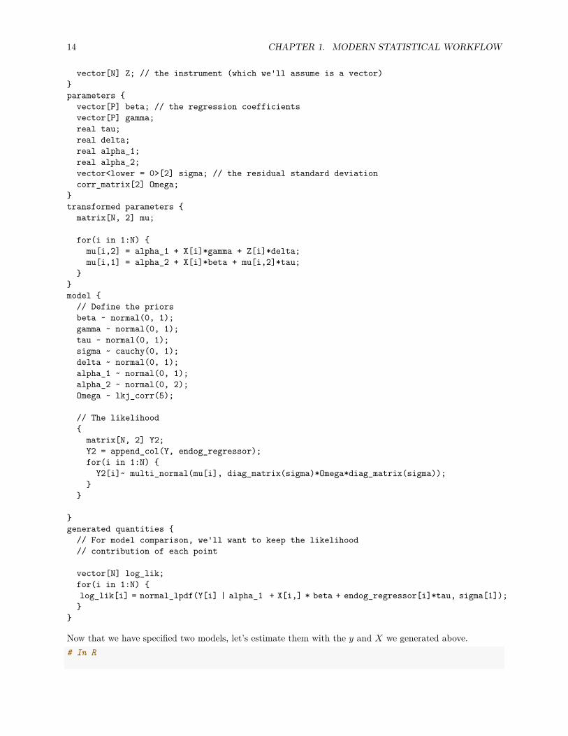
Now we define the correctly specified model. It is the same as above, but with a couple of changes:

// saved as models/joint_iv.stan// saved as models/joint_iv.standata int N; // number of observationsint P; // number of covariatesmatrix[N, P] X; //covariate matrixvector[N] Y; //outcome vectorvector[N] endog_regressor; // the endogenous regressor


vector[N] Z; // the instrument (which we'll assume is a vector)parameters vector[P] beta; // the regression coefficientsvector[P] gamma;real tau;real delta;real alpha_1;real alpha_2;vector<lower = 0>[2] sigma; // the residual standard deviationcorr_matrix[2] Omega;

transformed parameters matrix[N, 2] mu;

for(i in 1:N) mu[i,2] = alpha_1 + X[i]*gamma + Z[i]*delta;mu[i,1] = alpha_2 + X[i]*beta + mu[i,2]*tau;

model // Define the priorsbeta ~ normal(0, 1);gamma ~ normal(0, 1);tau ~ normal(0, 1);sigma ~ cauchy(0, 1);delta ~ normal(0, 1);alpha_1 ~ normal(0, 1);alpha_2 ~ normal(0, 2);Omega ~ lkj_corr(5);

// The likelihoodmatrix[N, 2] Y2;Y2 = append_col(Y, endog_regressor);for(i in 1:N) Y2[i]~ multi_normal(mu[i], diag_matrix(sigma)*Omega*diag_matrix(sigma));

generated quantities // For model comparison, we'll want to keep the likelihood// contribution of each point

vector[N] log_lik;for(i in 1:N) log_lik[i] = normal_lpdf(Y[i] | alpha_1 + X[i,] * beta + endog_regressor[i]*tau, sigma[1]);

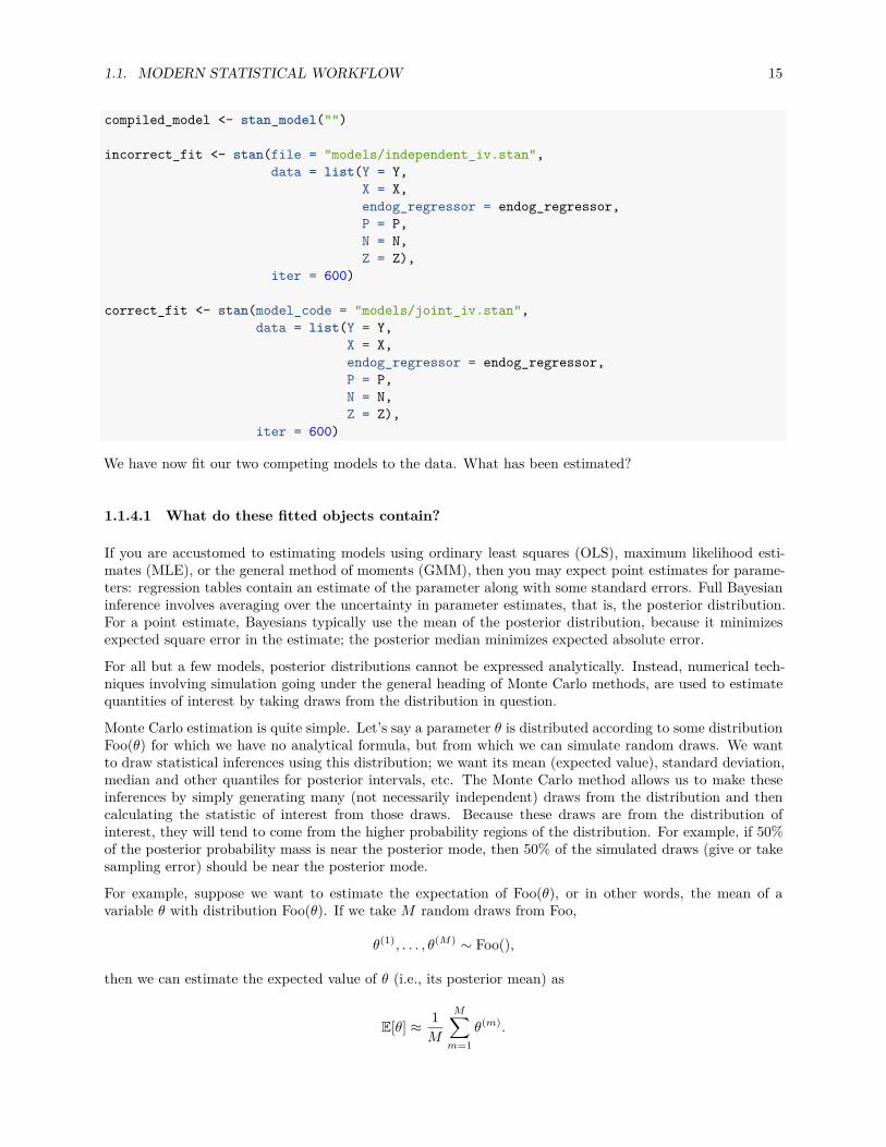
Now that we have specified two models, let’s estimate them with the y and X we generated above.# In R


compiled_model <- stan_model("")

incorrect_fit <- stan(file = "models/independent_iv.stan",data = list(Y = Y,

X = X,endog_regressor = endog_regressor,P = P,N = N,Z = Z),

iter = 600)

correct_fit <- stan(model_code = "models/joint_iv.stan",data = list(Y = Y,

X = X,endog_regressor = endog_regressor,P = P,N = N,Z = Z),

iter = 600)

We have now fit our two competing models to the data. What has been estimated?

1.1.4.1 What do these fitted objects contain?

If you are accustomed to estimating models using ordinary least squares (OLS), maximum likelihood esti-mates (MLE), or the general method of moments (GMM), then you may expect point estimates for parame-ters: regression tables contain an estimate of the parameter along with some standard errors. Full Bayesianinference involves averaging over the uncertainty in parameter estimates, that is, the posterior distribution.For a point estimate, Bayesians typically use the mean of the posterior distribution, because it minimizesexpected square error in the estimate; the posterior median minimizes expected absolute error.

For all but a few models, posterior distributions cannot be expressed analytically. Instead, numerical tech-niques involving simulation going under the general heading of Monte Carlo methods, are used to estimatequantities of interest by taking draws from the distribution in question.

Monte Carlo estimation is quite simple. Let’s say a parameter θ is distributed according to some distributionFoo(θ) for which we have no analytical formula, but from which we can simulate random draws. We wantto draw statistical inferences using this distribution; we want its mean (expected value), standard deviation,median and other quantiles for posterior intervals, etc. The Monte Carlo method allows us to make theseinferences by simply generating many (not necessarily independent) draws from the distribution and thencalculating the statistic of interest from those draws. Because these draws are from the distribution ofinterest, they will tend to come from the higher probability regions of the distribution. For example, if 50%of the posterior probability mass is near the posterior mode, then 50% of the simulated draws (give or takesampling error) should be near the posterior mode.

For example, suppose we want to estimate the expectation of Foo(θ), or in other words, the mean of avariable θ with distribution Foo(θ). If we take M random draws from Foo,

θ(1), . . . , θ(M) ∼ Foo(),

then we can estimate the expected value of θ (i.e., its posterior mean) as

E[θ] ≈ 1M

M∑m=1

θ(m).


If the draws θ(m) are independent, the result is a sequence of independent and identically distributed (i.i.d.)draws. The mean of a sequence of i.i.d. draws is governed by the central limit theorem, where the standarderror on the estimates is given by the standard deviation divided by the square root of the number of draws.Thus standard error decreases as O( 1√

M) in the number of independent draws M .

What makes Bayesian inference not only possible, but practical, is that almost all of the Bayesian inferencefor event probabilities, predictions, and parameter estimates can be expressed as expectations and carriedout using Monte Carlo methods.There is one hitch, though. For almost any practically useful model, not only will we not be able to getan analytical formula for the posterior, we will not be able to take independent draws. Fortunately, all isnot lost, as we will be able to take identically distributed draws using a technique known as Markov chainMonte Carlo (MCMC). With MCMC, the draws from a Markov chain in which each draw θ(m+1) depends(only) on the previous draw θ(m). Such draws are governed by the MCMC central limit theorem, wherein aquantity known as the effective sample size plays the role of the effective sample size in pure Monte Carloestimation. The effective sample size is determined by how autocorrelated the draws are; if each draw ishighly correlated with previous draws, then more draws are required to achieve the same effective samplesize.Stan is able to calculate the effective sample size for its MCMC methods and use that to estimate standarderrors for all of its predictive quantities, such as parameter and event probability estimates.A fitted Stan object contains a sequence of M draws, where each draw contains a value for every parameter(and generated quantity) in the model. If the computation has converged, as measured by built-in convergencediagnostics, the draws are from the posterior distribution of our parameters conditioned on the observeddata. These are draws from the joint posterior distribution; correlation between parameters is likely to bepresent in the joint posterior even if it was not present in the priors.In the generated quantities block of the two models above, we declare variables for two additional quantitiesof interest.

• The first, log_lik, is the log-likelihood, which we use for model comparison. We obtain this valuefor each parameter draw, for each value of yi. Thus if you have N observations and iter parameterdraws, this will contain N× iter log-likelihood values (which may produce a lot of output for largedata sets).

• The second, y_sim, is a posterior predictive quantity, in this case a replicated data set consisting of asequence of fresh outcomes generated randomly from the parameters. Rather than each observationhaving a “predicted value”, it has a predictive distribution that takes into account both the regressionresidual and uncertainty in the parameter estimates.

1.1.5 Model inspection

To address questions 1 and 2 above, we need to examine the parameter draws from the model to check fora few common problems:

• Lack of mixing. A poorly “mixing” Markov chain is one that moves very slowly between regions ofthe parameter space or barely moves at all. This can happen if the distribution of proposals is muchnarrower than the target (posterior) distribution or if it is much wider than the target distribution.In the former case most proposals will be accepted but the Markov chain will not explore the fullparameter space whereas in the latter case most proposals will be rejected and the chain will stall. Byrunning several Markov chains from different starting values we can see if each chain mixes well andif the chains are converging on a common distribution. If the chains don’t mix well then it’s unlikelywe’re sampling from a well specified posterior. The most common reason for this error is a poorlyspecified model.

• Stationarity. Markov chains should be covariance stationary, which means that the mean and varianceof the chain should not depend on when you draw the observations. Non-stationarity is normally theconsequence of a poorly specified model or an insufficient number of iterations.


• Autocorrelation. Especially in poorly specified or weakly identified models, a given draw of param-eters can be highly dependent on the previous draw of the parameters. One consequence of autocor-relation is that the posterior draws will contain less information than the number of draws suggests.That is, the effective posterior sample size will be much less than the actual posterior sample size. Forexample, 2000 draws with high autocorrelation will be less informative than 2000 independent draws.Assuming the model is specified correctly, then thinning (keeping only every k-th draw) is one commonapproach to dealing with highly autocorrelated draws. However, while thinning can reduce the auto-correlation in the draws that are retained it still sacrifices information. If possible, reparameterisingthe model is a better approach to this problem. (See section 21 of the manual, on Optimizing Stancode).

• Divergent transitions. In models with very curved or irregular posterior densities, we often get“divergent transitions”. This typically indicates that the sampler was unable to explore certain regionsof the distribution and a respecification or changes to the sampling routine may be required. Theeasiest way of addressing this issue is to use control = list(adapt_delta = 0.99) or some othernumber close to 1. This will lead to smaller step sizes and therefore more steps will be required toexplore the posterior. Sampling will be slower but the algorithm will often be better able to explorethese problematic regions, reducing the number of divergent transitions.

All of these potential problems can be checked using the ShinyStan graphical interface, which is availablein the shinystan R package. You can install it with install.packages("shinystan"), and run it withlaunch_shinystan(correct_fit). It will bring up an interactive session in your web browser within whichyou can explore the estimated parameters, examine the individual Markov chains, and check various diag-nostics. More information on ShinyStan is available here. We will confront most of these issues and showhow to resolve them in later chapters when we work with real examples. For now just keep in mind thatMCMC samples always need to be checked before they are used for making inferences.

1.1.6 Model comparison

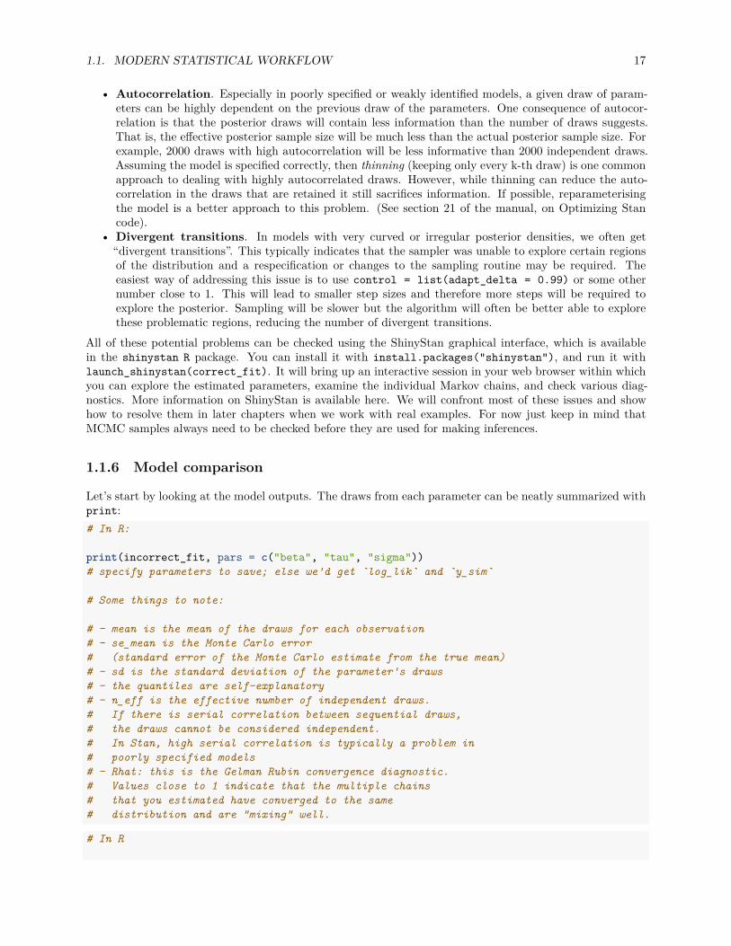
Let’s start by looking at the model outputs. The draws from each parameter can be neatly summarized withprint:# In R:

print(incorrect_fit, pars = c("beta", "tau", "sigma"))# specify parameters to save; else we'd get `log_lik` and `y_sim`

# Some things to note:

# - mean is the mean of the draws for each observation# - se_mean is the Monte Carlo error# (standard error of the Monte Carlo estimate from the true mean)# - sd is the standard deviation of the parameter's draws# - the quantiles are self-explanatory# - n_eff is the effective number of independent draws.# If there is serial correlation between sequential draws,# the draws cannot be considered independent.# In Stan, high serial correlation is typically a problem in# poorly specified models# - Rhat: this is the Gelman Rubin convergence diagnostic.# Values close to 1 indicate that the multiple chains# that you estimated have converged to the same# distribution and are "mixing" well.

# In R

http://mc-stan.org/documentation/

http://mc-stan.org/documentation/

http://mc-stan.org/interfaces/shinystan


print(correct_fit, pars = c("beta", "sigma", "nu"))

At the moment, it seems as though both our models have done about as good a job at estimating theregression coefficients β as one another. But the incorrectly specified model severely overestimates σ. Thismakes sense–a Student-t distribution with ν = 5 will have fat tails, and so a normal distribution will try toreplicate the extreme values by having a large variance.

How else might we compare the two models?

One approach is to use the loo package to compare the models on their estimated out-of-sample predictiveperformance. The idea of this package is to approximate each model’s leave-one-out (LOO) cross-validationerror, allowing model comparison by the LOO Information Criterion (LOOIC). LOOIC has the same purposeas the Akaike Information Criterion (AIC), which is to estimate the expected log predictive density (ELPD)for a new dataset. However, AIC ignores prior distributions and makes the assumption that the posterior is amultivariate normal distribution. The approach taken by the loo package does not make this distributionalassumption and also integrates over (averages over) the uncertainty in the parameters.

The Bayesian LOO estimate is∑N

n=1 log p(yn | y1, ..., yn−1, yn+1, ..., yN ), which requires fitting the model Ntimes, each time leaving out one of the N data points. For large datasets or complex models the compu-tational cost is usually prohibitive. The loo package does an approximation that avoids re-estimating themodel and requires only the log-likelihood evaluated at the posterior draws of the parameters. The approx-imation will be good so long as the posterior distribution is not very sensitive to leaving out any singleobservation.

A big upside of this approach is that it enables us to generate probabilistic estimates of the degree to whicheach model is most likely to produce the best out-of-sample predictions.

We use loo like so:# in R## library(loo) # Load the library## # Extract the log likelihoods of both models.# # Note that we need to declare log_lik in the generated quantities blockllik_incorrect <- extract_log_lik(incorrect_fit, parameter_name = "log_lik")llik_correct <- extract_log_lik(correct_fit, parameter_name = "log_lik")## # Estimate the leave-one-out cross validation errorloo_incorrect <- loo(llik_incorrect)loo_correct <- loo(llik_correct)

# # Print the LOO statisticsprint("Incorrect model")print(loo_incorrect)

print("Correct model")print(loo_correct)

The quantity elpd_loo is the expected log pointwise predictive density (ELPD). The log pointwise predictivedensity is easiest to understand in terms of its computation. For each data point we compute the log of itsaverage likelihood, where the average is computed over the posterior draws. Then we take the sum over allof the data points. We can multiply elpd_loo by −2 to calculate the looic, which you can think of like AICor BIC, but coming from our Bayesian framework. The −2 is not important; it simply converts the valueto the so-called deviance scale. The value of p_loo is the estimated effective number of parameters, whichis a measure of model complexity. The effective number of parameters can be substantially less than theactual number of parameters when there is strong dependence between parameters (e.g. in many hierarchicalmodels) or when parameters are given informative prior distributions. For further details on these quantities,

1.2. TOOLS OF THE TRADE: BORROWING FROM SOFTWARE ENGINEERING 19

please consult this paper.# Print the comparison between the two modelsprint(compare(loo_incorrect, loo_correct), digits = 2)

When using the compare function to compare two models the elpd_diff gives us the difference in theELPD estimates for the models. A positive elpd_diff indicates that the second model is estimated to havebetter out-of-sample predictive accuracy than the first, which is precisely what we expect in this case. Whencomparing more than two models the compare function will order the models by their ELPD estimates.

1.2 Tools of the trade: borrowing from software engineering

Building economic and statistical models increasingly requires sophisticated computation. This has thepotential to improve our modeling, but carries with it risks; as the complexity of our models grows, so toodoes the prospect of making potentially influential mistakes. The well-known spreadsheet error in Rogoffand Reinhart’s (Cite) paper—a fairly simple error in very public paper—was discovered. Who knows howmany other errors exist in more complex, less scruitinized work?Given the ease of making errors that substantively affect our models’ outputs, it makes sense to adopt aworkflow that minimizes the risk of such error happening. The set of tools discussed in this section, allborrowed from software engineering, are designed for this purpose. We suggest incorporating the followinginto your workflow:

• Document your code formally. At the very least, this will involve commenting your code to theextend where a colleague could read it and not have too many questions. Ideally it will include formaldocumentation of every function that you write.

• When you write functions, obey what we might call “Tinbergen’s rule of writing software”: one function,one objective. Try not to write omnibus functions that conduct a large part of your analysis. Writingsmall, modular functions will allow you to use unit testing, a framework that lets you run a set oftests automatically, ensuring that changing one part of your code base does not break other parts.

• Use Git to manage your workflow. Git is a very powerful tool that serves several purposes. It can helpyou back up your work, which is handy. It also allows you to view your codebase at periods when youcommitted some code to the code base. It lets you experiment on branches, without risking the main(“production”) code base. Finally helps you work in teams; formalizing a code-review procedure thatshould help catch errors.

http://arxiv.org/abs/1507.04544

Chapter 2

An introduction to hierarchicalmodeling

2.0.1 What is hierarchical modeling

Hierarchical modeling is the practice of building rich models, typcially in which each individual in yourdataset has their own set of parameters. Of course, without good prior information, this might not beidentified, or might be very weakly identified. Hierarchical modeling helps us deal with this problem byconsidering parameters at the low level as “sharing” information across individuals. This structure is knownas “partial pooling”. This session covers partial pooling, starting from the canonical example “8 schools”,then shows how you can use partial pooling to provide prior information when combining previous studieswith a new dataset. Finally I show how partial pooling can be used for analysis of panel data.

2.0.2 Why do hierarchical modeling?

There are a few excellent reasons to do hierarchical modeling:

To deal with unobserved information fairly fixed at the level of the group

The standard reason in economics to use panel data is to be able to “control for” confounding informationthat is fixed at the level of the individual over time. A similar motivation exists in hierarchical modeling.

The big difference is that we will not consider the individual or time effects to be fixed. Indeed, we routinely“shrink” effects towards a group-level average. This encodes the heuristic “death, taxes, and mean reversion”.Cross-validating your results will almost always show that such an approach is superior to fixed effects forprediction.

Prediction with high-dimensional categorical variables

Often in applied economics we have very high-dimensional categorical variables. For instance, plant, manager,project etc. This can massively increase the size of the parameter space, and result in over-fitting/poorgeneralization. In contrast, implementing high-dimensioned predictors as (shrunken) random effects typicallyresults in large improvements in predictive power.

Mr P: Multi-level regression and post-stratification

As economists we want to make inferences, typically of a causal nature. A common problem is that our dataare not collected randomly; we have some survey bias. Frequentists tend to correct for this by weightingobservations according to the inverse of their probability of being observed. Yet this approach moves awayfrom a generative model, making model comparison and validation difficult.

21

22 CHAPTER 2. AN INTRODUCTION TO HIERARCHICAL MODELING

Mr P is the practice of fitting a model in which individuals, or groups of individuals (say, grouped bydemographic cell) have their own sets of parameters (which are shrunk towards a hierarchical prior). Whenwe want to make an inference for a new population we only need to know its demographics. The inferenceis the weighted average across effects in the sample, with weights coming from the new population.

This method has the advantage that we can work with highly-biased samples, while keeping within a gen-erative framework (making Modern Statistical Workflow completely doable). In a notorious example, Mr Pwas used by David Rothschild at Microsoft Research to predict the outcome of the 2012 election based on asurvey run through the Xbox platform. The survey was almost entirely young men.

2.0.3 Exchangeability

Astute readers familiar with fixed effects models will have noted a problem with one of my arguments above.I said that we could use random intercepts to soak up unobserved information that affects both X and y byincluding group-varying intercepts αj . But this implies that the unobserved information fixed in a group,αj , is correlated with X. This correlation violates a very important rule in varying-intercept, varying-slopemodels: exchangeability.

Exchangeability says that there should be no information other than the outcome y that shouldallow us to distinguish the group to which a group-level parameter belongs.

In this example, we can clearly use values of X to predict j, violating exchangeability. But all is not lost.The group-varying parameter needs not be uncorrelated with X, only the random portion of it.

2.0.4 Conditional exchangeability and the Bafumi Gelman correction

Imagine we have an exchangability issue for a very simple model with only group-varying intercept: theunobserved information αj is correlated with Xi,j across groups. Let’s break αj down into its fixed andrandom portions.

αj = µ1 + ηj

whereηj ∼ normal(0, ση)

So that now the regression model can be written as

yi,t = µ1 + Xi,jβ + ei,j where ei,j = ϵi,j + ηj

For the correlation to hold, it must be the case that ηj is correlated with Xi,j . But our regression error is ei,j ,which is clearly correlated with X violating the Gauss-Markov theorem and so giving us biased estimates.

In a nice little paper Bafumi and Gelman suggest an elegant fix to this: simply control for group level averagesin the model of αj . This is a Bayesian take on what econometricians might know as a Mundlak/Chamberlainapproach. If Xj is the mean of Xi,j in group j, then we could use the model

αj = α + γXj + νj

which results in the correlaton between νj and Xi,j across groups being 0. It’s straightforward to implement,and gets you to conditional exchangeability—a condition under which mixed models like this one are valid.

http://www.stat.columbia.edu/~gelman/research/unpublished/Bafumi_Gelman_Midwest06.pdf

23

2.0.5 Exercise 1: Hierarchical priors

In this exercise we’ll estimate an experimental treatment effect using linear regression, while incorporatingprior information from previous studies. Rather than doing this in stages (estimating the treatment effectand then doing some meta-analysis), we’ll do everything in one pass. This has the advantage of helping usto get more precise estimates of all our model parameters.

2.0.6 A very basic underlying model

Let’s say that we run the J ’th experiment estimating the treatment effect of some treatment x on an outcomeY . It’s an expensive and ethically challenging experiment to run, so unfortunately we’re only able to get asample size of 20. For simplicity, we can assume that the treatment has the same treatment effect for allpeople, θ (this is easily dropped in more elaborate analyses). There have been J − 1 similar experiments runin the past. In this example our outcome data Y are conditionally normally distributed with (untreated)mean µ and standard deviation σ. There is nothing to stop us from having a far more complex model forthe data. So the outcome model looks like this:

yi,J ∼ Normal(µ + θJxi,J , σ)

The question is: how can we estimate the parameters of this model while taking account of the informationfrom the J − 1 previous studies? The answer is to use the so-called hierarchical prior.

2.0.7 The hierarchical prior

Let’s say that each of the J − 1 previous studies each has an estimated treatment effect βj , estimated withsome standard error sej . Taken together, are these estimates of βj the ground truth for the true treatmenteffect in their respective studies? One way of answering this is to ask ourselves: if the researchers of eachof those studies replicated their study in precisely the same way, but after checking the estimates estimatedby the other researchers, would they expect to find the same estimate they found before, βj? Or would theyperhaps expect some other treatment effect estimate, θj , that balances the information from their own studywith the other studies?The answer to this question gives rise to the hierarchical prior. In this prior, we say that the estimatedtreatment effect β is a noisy measure of the underlying treatment effect θj for each study j. These underlyingeffects are in turn noisy estimates of the true average treatment effect θ—noisy because of uncontrolled-forvaration across experiments. That is, if we make assumptions of normality:

βj ∼ Normal(θj , sej)

and

θj ∼ Normal(

θ, τ)

Where τ is the standard devation of the distribution of plausible experimental estimates.The analysis therefore has the following steps:

• Build a model of the treatment effects, considering our own study as another data point• Jointly estimate the hyperdistribution of treatment effects.

As an example, we’ll take the original 8-schools data, with some fake data for the experiment we want toestimate. The 8-schools example comes from an education intervention modeled by Rubin, in which a similarexperiment was conducted in 8 schools, with only treatment effects and their standard errors reported. The


task is to generate an estimate of the possible treatment effect that we might expect if we were to roll outthe program across all schools.library(rstan); library(dplyr); library(ggplot2); library(reshape2)

# The original 8 schools dataschools_dat <- data_frame(beta = c(28, 8, -3, 7, -1, 1, 18, 12),

se = c(15, 10, 16, 11, 9, 11, 10, 18))

# The known parameters of our data generating process for fake datamu <- 10sigma <- 5N <- 20# Our fake treatment effect estimate drawn from the posterior of the 8 schools exampletheta_J <- rnorm(1, 8, 6.45)

# Create some fake datatreatment <- sample(0:1, N, replace = T)y <- rnorm(N, mu + theta_J*treatment, sigma)

The Stan program we use to estimate the model is below. Note that these models can be difficult to fit, andso we employ a “reparameterization” below for the thetas. This is achieved by noticing that if

θj ∼ Normal(

θ, τ)

thenθj = θ + τzj

where zj ∼ Normal(0, 1). A standard normal has an easier geometry for Stan to work with, so this parame-terization of the model is typically preferred. Here is the Stan model:// We save this as 8_schools_w_regression.standata int<lower=0> J; // number of schoolsint N; // number of observations in the regression problemreal beta[J]; // estimated treatment effects from previous studiesreal<lower=0> se[J]; // s.e. of those effect estimatesvector[N] y; // the outcomes for students in our fake study datavector[N] treatment; // the treatment indicator in our fake study data

parameters real mu;real<lower=0> tau;real eta[J+1];real<lower = 0> sigma;real theta_hat;

transformed parameters real theta[J+1];for (j in 1:(J+1))theta[j] = theta_hat + tau * eta[j];

model // priors

25

tau ~ cauchy(5, 2);mu ~ normal(10, 2);eta ~ normal(0, 1);sigma ~ cauchy(3, 3);theta_hat ~ normal(8, 5);

// parameter model for previous studiesfor(j in 1:J) beta[j] ~ normal(theta[j], se[j]);

// our regressiony ~ normal(mu + theta[J+1]*treatment, sigma);

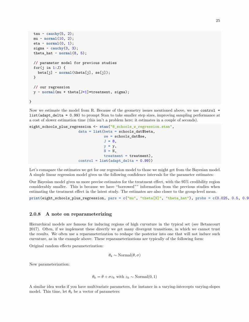
Now we estimate the model from R. Because of the geometry issues mentioned above, we use control =list(adapt_delta = 0.99) to prompt Stan to take smaller step sizes, improving sampling performance ata cost of slower estimation time (this isn’t a problem here; it estimates in a couple of seconds).eight_schools_plus_regression <- stan("8_schools_w_regression.stan",

data = list(beta = schools_dat$beta,se = schools_dat$se,J = 8,y = y,N = N,treatment = treatment),

control = list(adapt_delta = 0.99))

Let’s comapare the estimates we get for our regression model to those we might get from the Bayesian model.A simple linear regression model gives us the following confidence intervals for the parameter estimates:Our Bayesian model gives us more precise estimates for the treatment effect, with the 95% credibility regionconsiderably smaller. This is because we have “borrowed”” information from the previous studies whenestimating the treatment effect in the latest study. The estimates are also closer to the group-level mean.print(eight_schools_plus_regression, pars = c("mu", "theta[9]", "theta_hat"), probs = c(0.025, 0.5, 0.975))

2.0.8 A note on reparameterizing

Hierarchical models are famous for inducing regions of high curvature in the typical set (see Betancourt2017). Often, if we implement these directly we get many divergent transitions, in which we cannot trustthe results. We often use a reparameterization to reshape the posterior into one that will not induce suchcurvature, as in the example above. These reparameterizations are typically of the following form:Original random effects parameterization:

θk ∼ Normal(θ, σ)

New parameterization:

θk = θ + σzk with zk ∼ Normal(0, 1)

A similar idea works if you have multivariate parameters, for instance in a varying-intercepts varying-slopesmodel. This time, let θk be a vector of parameters:


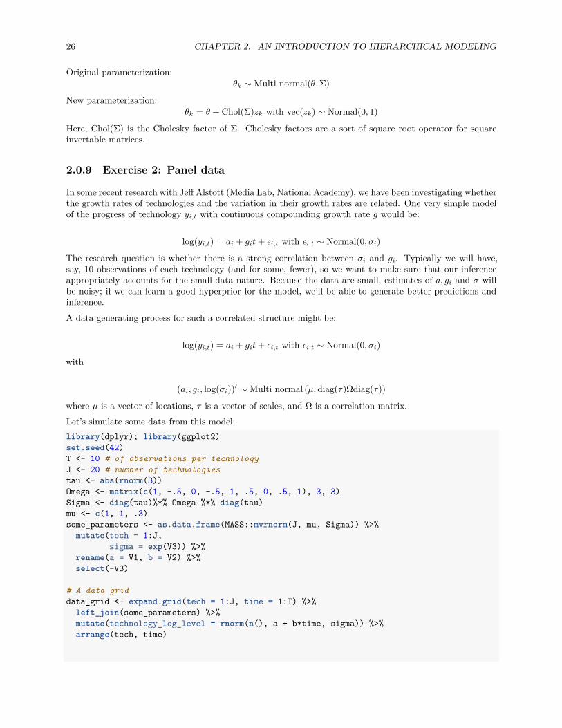
Original parameterization:θk ∼ Multi normal(θ, Σ)

New parameterization:θk = θ + Chol(Σ)zk with vec(zk) ∼ Normal(0, 1)

Here, Chol(Σ) is the Cholesky factor of Σ. Cholesky factors are a sort of square root operator for squareinvertable matrices.

2.0.9 Exercise 2: Panel data

In some recent research with Jeff Alstott (Media Lab, National Academy), we have been investigating whetherthe growth rates of technologies and the variation in their growth rates are related. One very simple modelof the progress of technology yi,t with continuous compounding growth rate g would be:

log(yi,t) = ai + git + ϵi,t with ϵi,t ∼ Normal(0, σi)

The research question is whether there is a strong correlation between σi and gi. Typically we will have,say, 10 observations of each technology (and for some, fewer), so we want to make sure that our inferenceappropriately accounts for the small-data nature. Because the data are small, estimates of a, gi and σ willbe noisy; if we can learn a good hyperprior for the model, we’ll be able to generate better predictions andinference.A data generating process for such a correlated structure might be:

log(yi,t) = ai + git + ϵi,t with ϵi,t ∼ Normal(0, σi)

with

(ai, gi, log(σi))′ ∼ Multi normal (µ, diag(τ)Ωdiag(τ))

where µ is a vector of locations, τ is a vector of scales, and Ω is a correlation matrix.Let’s simulate some data from this model:library(dplyr); library(ggplot2)set.seed(42)T <- 10 # of observations per technologyJ <- 20 # number of technologiestau <- abs(rnorm(3))Omega <- matrix(c(1, -.5, 0, -.5, 1, .5, 0, .5, 1), 3, 3)Sigma <- diag(tau)%*% Omega %*% diag(tau)mu <- c(1, 1, .3)some_parameters <- as.data.frame(MASS::mvrnorm(J, mu, Sigma)) %>%

mutate(tech = 1:J,sigma = exp(V3)) %>%

rename(a = V1, b = V2) %>%select(-V3)

# A data griddata_grid <- expand.grid(tech = 1:J, time = 1:T) %>%

left_join(some_parameters) %>%mutate(technology_log_level = rnorm(n(), a + b*time, sigma)) %>%arrange(tech, time)

27

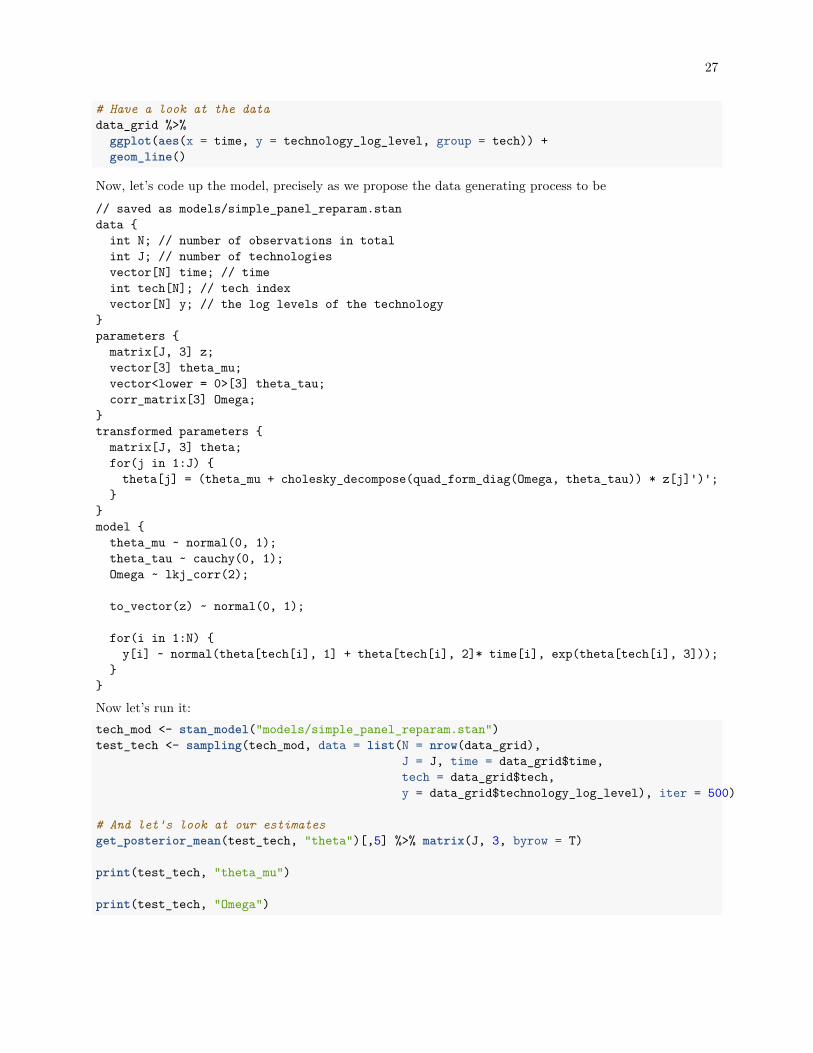
# Have a look at the datadata_grid %>%

ggplot(aes(x = time, y = technology_log_level, group = tech)) +geom_line()

Now, let’s code up the model, precisely as we propose the data generating process to be// saved as models/simple_panel_reparam.standata int N; // number of observations in totalint J; // number of technologiesvector[N] time; // timeint tech[N]; // tech indexvector[N] y; // the log levels of the technology

parameters matrix[J, 3] z;vector[3] theta_mu;vector<lower = 0>[3] theta_tau;corr_matrix[3] Omega;

transformed parameters matrix[J, 3] theta;for(j in 1:J) theta[j] = (theta_mu + cholesky_decompose(quad_form_diag(Omega, theta_tau)) * z[j]')';

model theta_mu ~ normal(0, 1);theta_tau ~ cauchy(0, 1);Omega ~ lkj_corr(2);

to_vector(z) ~ normal(0, 1);

for(i in 1:N) y[i] ~ normal(theta[tech[i], 1] + theta[tech[i], 2]* time[i], exp(theta[tech[i], 3]));

Now let’s run it:tech_mod <- stan_model("models/simple_panel_reparam.stan")test_tech <- sampling(tech_mod, data = list(N = nrow(data_grid),

J = J, time = data_grid$time,tech = data_grid$tech,y = data_grid$technology_log_level), iter = 500)

# And let's look at our estimatesget_posterior_mean(test_tech, "theta")[,5] %>% matrix(J, 3, byrow = T)

print(test_tech, "theta_mu")

print(test_tech, "Omega")

Chapter 3

Some fun time series models

3.1 This session

In this session, we’ll cover two of the things that Stan lets you do quite simply: implement state spacemodels, and finite mixtures.

3.1.1 Finite mixtures

In a post here, I describe a simple model in which each observation of our data could have one of twodensities. We estimated the parameters of both densities, and the probability of the data coming from either.While finite mixture models as in the last post are a useful learning aid, we might want richer models forapplied work. In particular, we might want the probability of our data having each density to vary acrossobservations. This is the first of two posts dedicated to this topic. I gave a talk covering some of this also(best viewed in Safari).For sake of an example, consider this: the daily returns series of a stock has two states. In the first, the stockis ‘priced to perfection’, and so the price is an I(1) random walk (daily returns are mean stationary). In thesecond, there is momentum—here, daily returns have AR(1) structure. Explicitly, for daily log returns rt:State 1: rt ∼ normal(α1, σ1)

State 2: rt ∼ normal(α2 + ρ1rt−1, σ2)

When we observe a value of rt, we don’t know for sure whether it came from the first or second model–thatis precisely what we want to infer. For this, we need a model for the probability that an observation camefrom each state st ∈ 1, 2. One such model could be:

prob(st = 1|It) = Logit−1(µt)

with

µt ∼ normal(α3 + ρ2µt−1 + f(It), σ3)

Here, f(It) is a function of the information available at the beginning of day t. If we had interestinginformation about sentiment, or news etc., it could go in here. For simplicity, let’s say f(It) = βrt−1.Under this specification (and for a vector containing all parameters, θ), we can specify the likelihood con-tribution of an observation. It is simply the weighted average of likelihoods under each candidate datagenerating process, where the weights are the probabilities that the data comes from each density.

29

https://modernstatisticalworkflow.blogspot.com/2016/10/finite-mixture-models-in-stan.html

https://dl.dropboxusercontent.com/u/63100926/become_a_bayesian_shareable.html

30 CHAPTER 3. SOME FUN TIME SERIES MODELS

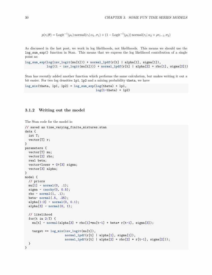
p(rt|θ) = Logit−1(µt) normal(rt| α1, σ1) + (1 − Logit−1(µt)) normal(rt| α2 + ρrt−1, σ2)

As discussed in the last post, we work in log likelihoods, not likelihoods. This means we should use thelog_sum_exp() function in Stan. This means that we express the log likelihood contribution of a singlepoint as:log_sum_exp(log(inv_logit(mu[t])) + normal_lpdf(r[t] | alpha[1], sigma[1]),

log((1 - inv_logit(mu[t]))) + normal_lpdf(r[t] | alpha[2] + rho[1], sigma[2]))

Stan has recently added another function which performs the same calculation, but makes writing it out abit easier. For two log densities lp1, lp2 and a mixing probability theta, we havelog_mix(theta, lp1, lp2) = log_sum_exp(log(theta) + lp1,

log(1-theta) + lp2)

3.1.2 Writing out the model

The Stan code for the model is:// saved as time_varying_finite_mixtures.standata int T;vector[T] r;

parameters vector[T] mu;vector[2] rho;real beta;vector<lower = 0>[3] sigma;vector[3] alpha;

model // priorsmu[1] ~ normal(0, .1);sigma ~ cauchy(0, 0.5);rho ~ normal(1, .1);beta~ normal(.5, .25);alpha[1:2] ~ normal(0, 0.1);alpha[3] ~ normal(0, 1);

// likelihoodfor(t in 2:T) mu[t] ~ normal(alpha[3] + rho[1]*mu[t-1] + beta* r[t-1], sigma[3]);

target += log_mix(inv_logit(mu[t]),normal_lpdf(r[t] | alpha[1], sigma[1]),normal_lpdf(r[t] | alpha[2] + rho[2] * r[t-1], sigma[2]));

3.1. THIS SESSION 31

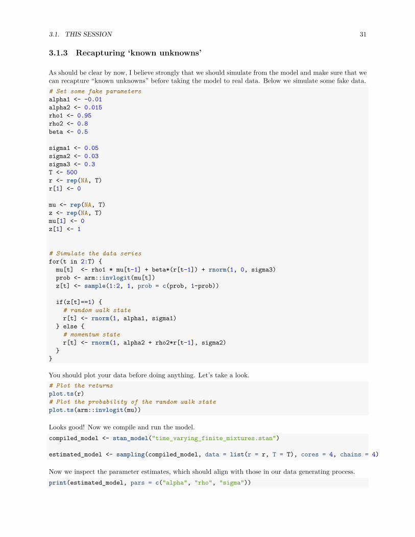
3.1.3 Recapturing ‘known unknowns’

As should be clear by now, I believe strongly that we should simulate from the model and make sure that wecan recapture “known unknowns” before taking the model to real data. Below we simulate some fake data.# Set some fake parametersalpha1 <- -0.01alpha2 <- 0.015rho1 <- 0.95rho2 <- 0.8beta <- 0.5

sigma1 <- 0.05sigma2 <- 0.03sigma3 <- 0.3T <- 500r <- rep(NA, T)r[1] <- 0

mu <- rep(NA, T)z <- rep(NA, T)mu[1] <- 0z[1] <- 1

# Simulate the data seriesfor(t in 2:T) mu[t] <- rho1 * mu[t-1] + beta*(r[t-1]) + rnorm(1, 0, sigma3)prob <- arm::invlogit(mu[t])z[t] <- sample(1:2, 1, prob = c(prob, 1-prob))

if(z[t]==1) # random walk stater[t] <- rnorm(1, alpha1, sigma1)

else # momentum stater[t] <- rnorm(1, alpha2 + rho2*r[t-1], sigma2)

You should plot your data before doing anything. Let’s take a look.# Plot the returnsplot.ts(r)# Plot the probability of the random walk stateplot.ts(arm::invlogit(mu))

Looks good! Now we compile and run the model.compiled_model <- stan_model("time_varying_finite_mixtures.stan")

estimated_model <- sampling(compiled_model, data = list(r = r, T = T), cores = 4, chains = 4)

Now we inspect the parameter estimates, which should align with those in our data generating process.print(estimated_model, pars = c("alpha", "rho", "sigma"))


It seems that most of the parameters appear to have estimated quite cleanly–most of the Rhats are fairlyclose, to 1, with the exception of the standard deviation of the updates in the latent series (which will bevery weakly identified, given we don’t observe mu). We would fix this by adding better prior information tothe model.

3.1.4 Taking the model to real data

Now we know that our program can recapture a known model, we can take it to some real data. In this case,we’ll use the log differences in sequential adjusted closing prices for Apple’s common stock. With Applebeing such a large, well-researched (and highly liquid) stock, we should expect that it spends almost all timein the random walk state. Let’s see what the data say!# Now with real data!aapl <- Quandl::Quandl("YAHOO/AAPL")

aapl <- aapl %>%mutate(Date = as.Date(Date)) %>%arrange(Date) %>%mutate(l_ac = log(`Adjusted Close`),

dl_ac = c(NA, diff(l_ac))) %>%filter(Date > "2015-01-01")

aapl_mod <- sampling(compiled_model, data= list(T = nrow(aapl), r = aapl$dl_ac*100))

Now check that the model has fit properlyshinystan::launch_shinystan(aapl_mod)

And finally plot the probability of being in each state.plot1 <- aapl_mod %>%

as.data.frame() %>%select(contains("mu")) %>%melt() %>%group_by(variable) %>%summarise(lower = quantile(value, 0.95),

median = median(value),upper = quantile(value, 0.05)) %>%

mutate(date = aapl$Date,ac = aapl$l_ac) %>%

ggplot(aes(x = date)) +geom_ribbon(aes(ymin = arm::invlogit(lower), ymax = arm::invlogit(upper)), fill= "orange", alpha = 0.4) +geom_line(aes(y = arm::invlogit(median))) +ggthemes::theme_economist() +xlab("Date") +ylab("Probability of random walk model")

plot2 <- aapl_mod %>%as.data.frame() %>%select(contains("mu")) %>%melt() %>%group_by(variable) %>%summarise(lower = quantile(value, 0.95),

median = median(value),

3.2. A STATE SPACE MODEL INVOLVING POLLS 33

upper = quantile(value, 0.05)) %>%mutate(date = aapl$Date,

ac = aapl$`Adjusted Close`) %>%ggplot(aes(x = date, y = ac)) +geom_line() +ggthemes::theme_economist() +xlab("Date") +ylab("Adjusted Close")

gridExtra::grid.arrange(plot1, plot2)

And there we go! As expected, Apple spends almost all their time in the random walk state, but, surprisingly,appears to have had a few periods with some genuine (mainly negative) momentum.

3.1.5 Building up the model

The main problem with this model is that our latent state µ can only really vary so much from period toperiod. That can delay the response to the appearance of a new state, and slow the process of “flippingback” into the regular state. One way of getting around this is to have a discrete state with more flexibilityin flipping between states. We’ll explore this in the next post, on Regime-Switching models.

3.2 A state space model involving polls

This tutorial covers how to build a low-to-high frequency interpolation model in which we have possiblymany sources of information that occur at various frequencies. The example I’ll use is drawing inferenceabout the preference shares of Clinton and Trump in the current presidential campaign. This is a goodexample for this sort of imputation:

• Data (polls) are sporadically released. Sometimes we have many released simultaneously; at othertimes there may be many days with no releases.

• The various polls don’t necessarily agree. They might have different methodologies or sampling issues,resulting in quite different outcomes. We want to build a model that can incorporate this.

There are two ingredients to the polling model. A multi-measurement model, typified by Rubin’s 8 schoolsexample. And a state-space model. Let’s briefly describe these.

3.2.1 Multi-measurement model and the 8 schools example

Let’s say we run a randomized control trial in 8 schools. Each school i reports its own treatment effect tei,which has a standard error σi. There are two questions the 8-schools model tries to answer:

• If you administer the experiment at one of these schools, say, school 1, and have your estimate of thetreatment effect te1, what do you expect would be the treatment effect if you were to run the experimentagain? In particular, would your expectations of the treatment effect in the next experiment changeonce you learn the treatment effects estimated from the experiments in the other schools?

• If you roll out the experiment at a new school (school 9), what do we expect the treatment effect tobe?

The statistical model that Rubin proposed is that each school has its own true latent treatment effect yi,around which our treatment effects are distributed.

tei ∼ N (yi, σi)


These “true” but unobserved treatment effects are in turn distributed according to a common hyper-distribution with mean µ and standard deviation τ

yi ∼ N (µ, τ)

Once we have priors for µ and τ , we can estimate the above model with Bayesian methods.

3.2.2 A state-space model

State-space models are a useful way of dealing with noisy or incomplete data, like our polling data. The ideais that we can divide our model into two parts:

• The state. We don’t observe the state; it is a latent variable. But we know how it changes throughtime (or at least how large its potential changes are).

• The measurement. Our state is measured with imprecision. The measurement model is the distri-bution of the data that we observe around the state.

A simple example might be consumer confidence, an unobservable latent construct about which our surveyresponses should be distributed. So our state-space model would be:

The state

conft ∼ N (conft−1, σ)

which simply says that consumer confidence is a random walk with normal innovations with a standarddeviation σ, and

survey measuret ∼ normal(conft, τ)

which says that our survey measures are normally distributed around the true latent state, with standarddeviation τ .

Again, once we provide priors for the initial value of the state conf0 and τ , we can estimate this model quiteeasily.

The important thing to note is that we have a model for the state even if there is no observed measurement.That is, we know (the distribution for) how consumer confidence should progress even for the periods inwhich there are no consumer confidence surveys. This makes state-space models ideal for data with irregularfrequencies or missing data.

3.2.3 Putting it together

As you can see, these two models are very similar: they involve making inference about a latent quantityfrom noisy measurements. The first shows us how we can aggregate many noisy measurements togetherwithin a single time period, while the second shows us how to combine irregular noisy measures over time.We can now combine these two models to aggregate multiple polls over time.

The data generating process I had in mind is a very simple model where each candidate’s preference shareis an unobserved state, which polls try to measure. Unlike some volatile poll aggregators, I assume that theunobserved state can move according to a random walk with normal disturbances of standard deviation .25%.This greatly smoothes out the sorts of fluctuations we see around the conventions etc. We could estimatethis parameter using fairly tight priors, but I just hard-code it in for simplicity.

That is, we have the state for candidate c in time t evolving according to


Vote sharec,t ∼ N (Vote sharec,t−1.0.25)

with measurements being made of this in the polls. Each poll p at time t is distributed according to

pollc,p,t ∼ N (Vote sharec,t.τ)

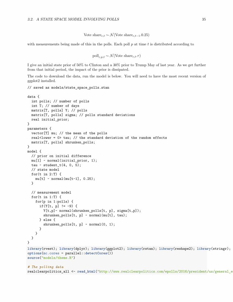
I give an initial state prior of 50% to Clinton and a 30% prior to Trump May of last year. As we get furtherfrom that initial period, the impact of the prior is dissipated.The code to download the data, run the model is below. You will need to have the most recent version ofggplot2 installed.// saved as models/state_space_polls.stan

data int polls; // number of pollsint T; // number of daysmatrix[T, polls] Y; // pollsmatrix[T, polls] sigma; // polls standard deviationsreal initial_prior;

parameters vector[T] mu; // the mean of the pollsreal<lower = 0> tau; // the standard deviation of the random effectsmatrix[T, polls] shrunken_polls;

model // prior on initial differencemu[1] ~ normal(initial_prior, 1);tau ~ student_t(4, 0, 5);// state modelfor(t in 2:T) mu[t] ~ normal(mu[t-1], 0.25);

// measurement modelfor(t in 1:T) for(p in 1:polls) if(Y[t, p] != -9) Y[t,p]~ normal(shrunken_polls[t, p], sigma[t,p]);shrunken_polls[t, p] ~ normal(mu[t], tau);

else shrunken_polls[t, p] ~ normal(0, 1);

library(rvest); library(dplyr); library(ggplot2); library(rstan); library(reshape2); library(stringr); library(lubridate)options(mc.cores = parallel::detectCores())source("models/theme.R")

# The polling datarealclearpolitics_all <- read_html("http://www.realclearpolitics.com/epolls/2016/president/us/general_election_trump_vs_clinton-5491.html#polls")


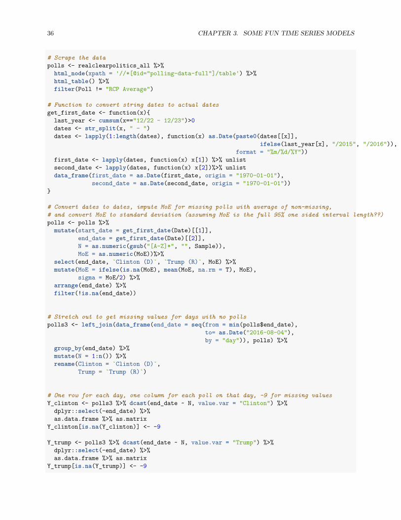
# Scrape the datapolls <- realclearpolitics_all %>%

html_node(xpath = '//*[@id="polling-data-full"]/table') %>%html_table() %>%filter(Poll != "RCP Average")

# Function to convert string dates to actual datesget_first_date <- function(x)last_year <- cumsum(x=="12/22 - 12/23")>0dates <- str_split(x, " - ")dates <- lapply(1:length(dates), function(x) as.Date(paste0(dates[[x]],

ifelse(last_year[x], "/2015", "/2016")),format = "%m/%d/%Y"))

first_date <- lapply(dates, function(x) x[1]) %>% unlistsecond_date <- lapply(dates, function(x) x[2])%>% unlistdata_frame(first_date = as.Date(first_date, origin = "1970-01-01"),

second_date = as.Date(second_date, origin = "1970-01-01"))

# Convert dates to dates, impute MoE for missing polls with average of non-missing,# and convert MoE to standard deviation (assuming MoE is the full 95% one sided interval length??)polls <- polls %>%

mutate(start_date = get_first_date(Date)[[1]],end_date = get_first_date(Date)[[2]],N = as.numeric(gsub("[A-Z]*", "", Sample)),MoE = as.numeric(MoE))%>%

select(end_date, `Clinton (D)`, `Trump (R)`, MoE) %>%mutate(MoE = ifelse(is.na(MoE), mean(MoE, na.rm = T), MoE),

sigma = MoE/2) %>%arrange(end_date) %>%filter(!is.na(end_date))

# Stretch out to get missing values for days with no pollspolls3 <- left_join(data_frame(end_date = seq(from = min(polls$end_date),

to= as.Date("2016-08-04"),by = "day")), polls) %>%

group_by(end_date) %>%mutate(N = 1:n()) %>%rename(Clinton = `Clinton (D)`,

Trump = `Trump (R)`)

# One row for each day, one column for each poll on that day, -9 for missing valuesY_clinton <- polls3 %>% dcast(end_date ~ N, value.var = "Clinton") %>%dplyr::select(-end_date) %>%as.data.frame %>% as.matrix

Y_clinton[is.na(Y_clinton)] <- -9

Y_trump <- polls3 %>% dcast(end_date ~ N, value.var = "Trump") %>%dplyr::select(-end_date) %>%as.data.frame %>% as.matrix

Y_trump[is.na(Y_trump)] <- -9


# Do the same for margin of errors for those pollssigma <- polls3 %>% dcast(end_date ~ N, value.var = "sigma")%>%dplyr::select(-end_date)%>%as.data.frame %>% as.matrix

sigma[is.na(sigma)] <- -9

# Run the two models

clinton_model <- stan("models/state_space_polls.stan",data = list(T = nrow(Y_clinton),

polls = ncol(Y_clinton),Y = Y_clinton,sigma = sigma,initial_prior = 50), iter = 600)

trump_model <- stan("models/state_space_polls.stan",data = list(T = nrow(Y_trump),

polls = ncol(Y_trump),Y = Y_trump,sigma = sigma,initial_prior = 30), iter = 600)

# Pull the state vectors

mu_clinton <- extract(clinton_model, pars = "mu", permuted = T)[[1]] %>%as.data.frame

mu_trump <- extract(trump_model, pars = "mu", permuted = T)[[1]] %>%as.data.frame

# Rename to get datesnames(mu_clinton) <- unique(paste0(polls3$end_date))names(mu_trump) <- unique(paste0(polls3$end_date))

# summarise uncertainty for each date

mu_ts_clinton <- mu_clinton %>% melt %>%mutate(date = as.Date(variable)) %>%group_by(date) %>%summarise(median = median(value),

lower = quantile(value, 0.025),upper = quantile(value, 0.975),candidate = "Clinton")

mu_ts_trump <- mu_trump %>% melt %>%mutate(date = as.Date(variable)) %>%group_by(date) %>%summarise(median = median(value),

lower = quantile(value, 0.025),


upper = quantile(value, 0.975),candidate = "Trump")

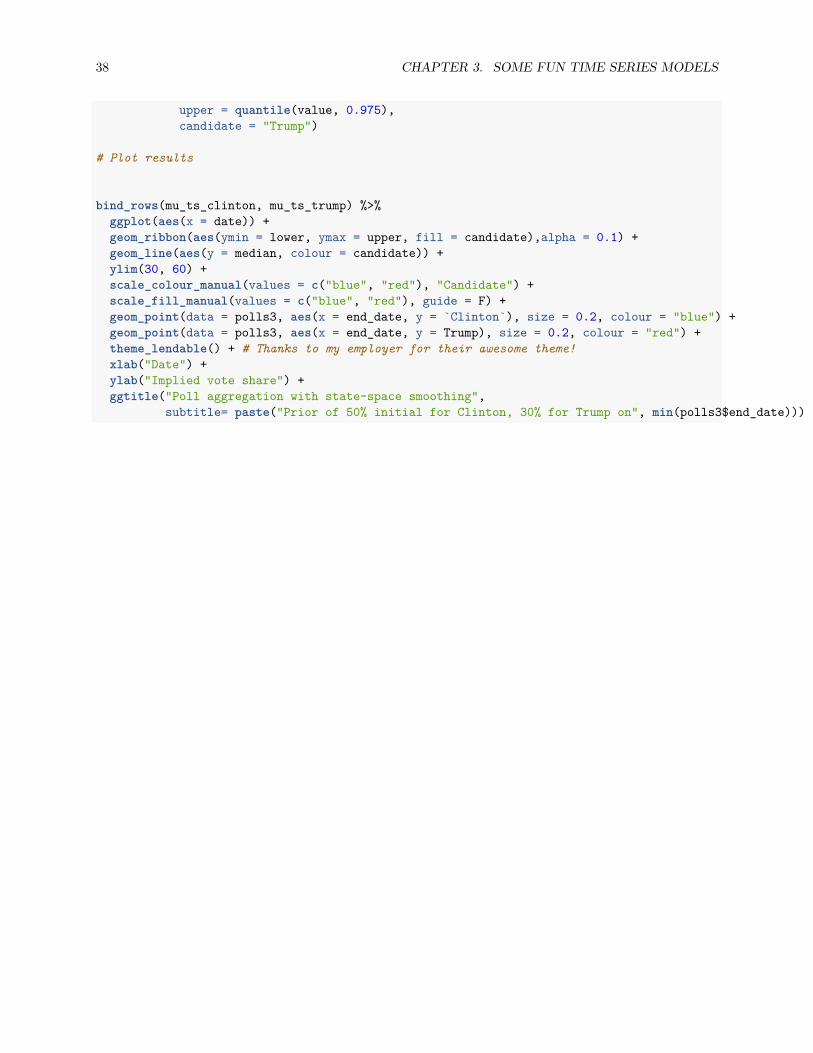
# Plot results

bind_rows(mu_ts_clinton, mu_ts_trump) %>%ggplot(aes(x = date)) +geom_ribbon(aes(ymin = lower, ymax = upper, fill = candidate),alpha = 0.1) +geom_line(aes(y = median, colour = candidate)) +ylim(30, 60) +scale_colour_manual(values = c("blue", "red"), "Candidate") +scale_fill_manual(values = c("blue", "red"), guide = F) +geom_point(data = polls3, aes(x = end_date, y = `Clinton`), size = 0.2, colour = "blue") +geom_point(data = polls3, aes(x = end_date, y = Trump), size = 0.2, colour = "red") +theme_lendable() + # Thanks to my employer for their awesome theme!xlab("Date") +ylab("Implied vote share") +ggtitle("Poll aggregation with state-space smoothing",

subtitle= paste("Prior of 50% initial for Clinton, 30% for Trump on", min(polls3$end_date)))

Bibliography

39

a brief introduction to econometrics in stan - github pages · these notes are for a one-day short...

Documents