1

A Capacitated Facility Location Problem with Constrained Backlogging Probabilities

Francisco José Ferreira Silva (corresponding author)

GREL, IET, Universitat Pompeu Fabra Ramon Trias Fargas, 25-27, 08005 Barcelona, Spain

CEEAplA, Universidade dos Açores Rua da Mãe de Deus, 9502 Ponta Delgada, Portugal

Telephone: (+351) 296 650 555 Fax: (+351) 296 650 083

email: francisco.silva@upf.edu

Daniel Serra

GREL, IET, Universitat Pompeu Fabra Ramon Trias Fargas, 25-27, 08005 Barcelona, Spain

Telephone: (+34) 93 542 1666 Fax: (+34) 93 542 1746

email: daniel.serra@upf.edu

2

Abstract One of the assumptions of the Capacitated Facility Location Problem (CFLP) is that

demand is known and fixed. Most often, this is not the case when managers take some

strategic decisions such as locating facilities and assigning demand points to those

facilities. In this paper we consider demand as stochastic and we model each of the

facilities as an independent queue. Stochastic models of manufacturing systems and

deterministic location models are put together in order to obtain a formula for the

backlogging probability at a potential facility location.

Several solution techniques have been proposed to solve the CFLP. One of the most

recently proposed heuristics, a Reactive Greedy Adaptive Search Procedure, is

implemented in order to solve the model formulated. We present some computational

experiments in order to evaluate the heuristics’ performance and to illustrate the use of

this new formulation for the CFLP. The paper finishes with a simple simulation

exercise.

Keywords: Location, queuing, greedy heuristics, simulation. JEL: C61, L80

3

1. Introduction

Transportation costs and location-specific fixed costs are often a major

component of the price (cost) of goods. The Facility Location Problem (FLP),

introduced by (Balinski 1965) addresses the problem of locating a new set of facilities

in such a way that the sum of those two costs is minimized.

Another concern when designing and operating a manufacturing system is the

capacity the system tolerates: given the processing facilities, what is the maximum rate

of order receipt that can be accepted so that all the orders can be satisfied? The

Capacitated Facility Location Problem (CFLP) is a variant of the FLP, which includes

capacities for the facilities. With the inclusion of the capacities, an open facility that is

the least cost source for a demand node may not be able to serve any of the demand at

that node.

The capacities of the facilities as well as the demand at each of the demand

nodes have been assumed to be known deterministic parameters. In this paper we relax

these assumptions by considering that the demand is stochastic following a given

probability distribution and where capacity at each facility results from the probability

of losing or backlogging the demand.

Stochastic models on manufacturing systems give us some important results,

using analytical techniques such as stochastic processes, queuing theory and reliability

theory, which allow the computation of the referred probabilities as a function of arrival

and service rates. In this paper we introduce these considerations in the CFLP. The

objective is to find the best location of facilities (the one that minimizes total

transportation and fixed costs) maintaining the probability of losing /backlogging

demand on a small level.

4

The CFLP considers that distinct potential facility sites present different fixed

costs for locating a facility, that facilities being sited are constrained to a given capacity

level on the demand they can serve and that we do not know, a priori, the optimal

number of facilities to be opened. These assumptions make from the CFLP a complex

problem that is difficult to solve. There is a vast literature concerning the development

and testing of new algorithms that search for the solution to the problem.

The most common approach to solving the CFLP is the use of Lagrangean

heuristics. These heuristics are based on a Lagrangean relaxation and some method for

solving the Lagrangean dual problem. More recently Greedy Heuristics, Tabu Search

and Genetic Algorithms have been proposed to solve the CFLP. Based on previous

research we will propose a heuristic algorithm to solve the new version of the model.

The paper is organized as follows: in section 2 we describe the Single Source

Capacitated Facility Location Problem; in section 3 we give a brief description of

stochastic manufacturing models whose results are to be used in section 4 in order to

formulate the Queue Length Capacitated Facility Location Problem. In section 5 we

describe heuristics to solve the problem and finally in section 6 we offer some

numerical examples.

The motivation for the paper results from the fact that this model may allow a

rapid analysis of many manufacturing alternatives enabling the firm to take rapid

decisions both in the design and in the operation phases, and to obtain some competitive

advantages in costs resulting from vantages on the stock management policy.

2. The Single Source Capacitated Facility Location Problem (SSCFLP)

Facility Location Problems (FLP) deserved a special place in Location Literature

in the second half of last century. Some important summaries of the state of the art can

5

be found in (Balinski and Spielberg, 1969), (ReVelle et al., 1970), (Guignard and

Spielberg, 1977), (Cornuejols, 1978) or (Krarup and Pruzan, 1983).

The FLP derives its name from the analogy to decision problems concerning the

location of plants or facilities (e.g. factories, warehouses, schools) so as to minimize the

total cost of serving clients (e.g. depots, retail outlets, students). (Krarup and Pruzan,

1983) refer their own experience as consultants where they have utilized FLP

formulations as the basis for providing decision inputs to real-world problems regarding

the number, size, design, location, and service patterns for such widely varied ‘plants’

as high-schools, hospitals, silos, slaughterhouses, electronic components, warehouses,

as well as traditional production plants. As referred by the same authors the FLP permits

in a sense the broadest framework. Neither the number of plants to be located nor the

transportation or communication pattern is predetermined. Furthermore, the basic

formulation of FLP lends itself readily to sensitivity analyses. In addition, FLP invites

modifications which may permit more ‘realistic’ modeling. While FLP is basically a

discrete, static, deterministic, one-product, fixed-plus-linear costs minimization problem

formulation, it can be modified to accommodate dynamic, stochastic, multi-product,

nonlinear cost minimization formulations.

The first explicit formulation of FLP is frequently attributed to (Balinski, 1966)

whose expository article on integer programming includes the mixed-integer

formulation. The paper was presented at the IBM Scientific Symposium on

Combinatorial Problems in March 1964 but remained unpublished until 1966. However,

FLP’s are also dealt with in the pioneering papers by (Kuehn and Hamburger, 1963) and

(Manne, 1964).

6

FLP, Plant Location Problems consider situations in which a commodity is

supplied from a subset of plants, selected from a set of potential location sites, to satisfy

the demand of a set of clients. There are fixed costs for opening the plants and

transportation costs to supply the commodity or the standard product-mix from potential

location sites to clients. The decision maker seeks for a combination of minimum costs

in terms of the plants to be opened and the allocation of clients within the subset of open

plants.

The simplest formulation of FLP is the Uncapacitated Facility Location Problem

(UFLP). It considers that the plants have unlimited capacity. There are several

application for the UFLP, for example, bank account location (Cornuejols et al., 1977),

economic lot sizing (Krarup and Blide, 1977), machine scheduling (Hansen and

Kaufman) or portfolio management (Beck and Mulvey).

Let { }m,...,1I = be a set of customers which are to be served from plants located in

a subset of sites from a given set { }n,...,1J = of potential sites. For each site Jj ∈ , the

fixed cost of opening the plant at j is jf . The cost of assigning site j to customer i isijc .

Considering,

=otherwise 0

icustomer serves jfacility if 1ijX

=otherwise 0

opened is jfacility if 1jY

the model can be formulated as follows:

7

{ }{ } j Y

j i, X

j i, YX

i X

ts

YfXc min

j

ij

jij

n

jij

m

1i

n

jjj

n

jijij

∀∈

∀∀∈

∀∀≤−

∀=

+

∑

∑ ∑∑

=

= ==

1,0

1,0

0

1

..

1

11

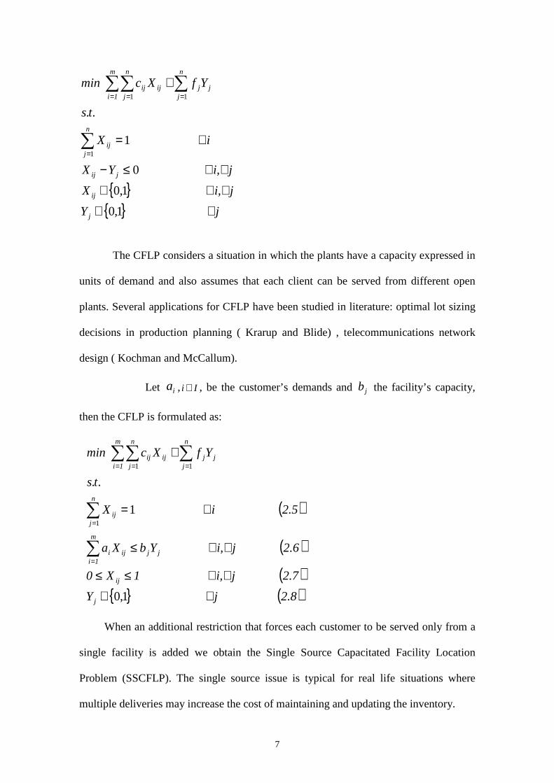
The CFLP considers a situation in which the plants have a capacity expressed in

units of demand and also assumes that each client can be served from different open

plants. Several applications for CFLP have been studied in literature: optimal lot sizing

decisions in production planning ( Krarup and Blide) , telecommunications network

design ( Kochman and McCallum).

Let ia , Ii ∈ , be the customer’s demands and jb the facility’s capacity,

then the CFLP is formulated as:

( )

( )

( ){ } ( ) 2.8 j Y

2.7 j i, 1X0

2.6 j i, YbXa

2.5 i X

ts

YfXc min

j

ij

m

1ijjiji

n

jij

m

1i

n

jjj

n

jijij

∀∈

∀∀≤≤

∀∀≤

∀=

+

∑

∑

∑ ∑∑

=

=

= ==

1,0

1

..

1

11

When an additional restriction that forces each customer to be served only from a

single facility is added we obtain the Single Source Capacitated Facility Location

Problem (SSCFLP). The single source issue is typical for real life situations where

multiple deliveries may increase the cost of maintaining and updating the inventory.

8

This problem is in general more difficult to solve because the decision variables

are binary. Another assumption of the SSCFLP considers that transportation costs from

facilities to markets are linear according to the quantity transported (i.e., there are no

economies of scale and the production costs at a facility are linear in the quantity

produced once an initial fixed cost has been incurred). This problem has been widely

studied in the literature, and for review purposes, see as an example Sridharan (1995).

The objective function minimizes the cost of assigning customers to open facilities

and the cost of establishing such facilities. Constraint set 2.9 can be referred to as the

capacity constraints (or the facility constraint), and ensures that the customer demand

served by a certain facility does not exceed its capacity. Constraint set 2.10 can be

referred to as the demand constraints (or the customer constraints), and ensures that

each customer is assigned to exactly one facility. Finally, constraint set 2.11 ensures that

the assignments are made only to open facilities. In this model all decision variables are

binary.

Constraint set 2.9 and constraint set 2.11 may be concentrated in the following

constraint:

{ }{ } (2.13) j Y

(2.12) j i, X

(2.11) j i, YX

(2.10) i X

(2.9) j bXa

ts

YfXc min

j

ij

jij

n

jij

m

ijiji

m

1i

n

jjj

n

jijij

∀∈

∀∀∈

∀∀≤−

∀=

∀≤

+

∑

∑

∑ ∑∑

=

=

= ==

1,0

1,0

0

1

..

1

1

11

9

(2.12) j YbXam

ijjiji ∀≤∑

=1

Nevertheless, in order to facilitate the formulation of the new model we will keep

the initial configuration.

3. Stochastic Models for Manufacturing Systems Stochastic models for manufacturing systems have been developed for more

than half a century. These models were developed as an attempt to provide analytical

formulas that would predict the performance of manufacturing systems. For a good

review see (Suri et al. 1993). Models which explicitly make use of queuing theory were

first developed to solve machine interference problems. Interference problems result

from the non-synchronized use of the machines and are concretized when down

machines are interfering with operating ones. Queuing theory is the most common

methodology for solving this type of problems. For a good review on early models, see

(Stecke et al. 1985), and for a detailed mathematical description of the models and their

applications see (Buzacott et al. 1993).

The two traditional forms of organizing manufacturing systems are the job shop

and the flow lines. The main difference between the two forms consists of the fact that

the flow lines system requires all jobs to visit all machines and work centres in the same

sequence which is not the case in the job shops, where we may alter the sequence. Job

shops obey to two different configurations: produce-to-order, where the job order

arrives from outside the shop (stocks are not allowed) and produce-to-stock, where the

job orders will be influenced by the stock levels. In this paper we are concerned with

produce-to-stock systems. Produce-to-stock operations should reduce the delay in filling

customer’s orders and may lead to increased sales. The cost of keeping inventories is

10

also expected to be higher with this system leading to the need for careful stock

management.

‘System design’ is the term used to specify the rules that determine how

production authorizations are generated. In this paper we restrict the discussion to single

stage manufacturing facilities. Completed items of each product are kept in an output

store. As customers arrive, their demands are met by delivering to them items from the

output store. If all demands cannot be met immediately, two alternatives will be

considered: lost sales and back-logged demand (where the customer waits until his

required demand is met).

Now, consider the well known Production Authorization (PA) Cards System. In

a simple formula the system works as follows: each item produced by the

manufacturing facility has a tag associated, and when an item of a given product is

delivered to a customer the tag is removed and becomes a production authorization or

PA card for that product. The PA card can be directed to the production facility as soon

as it is generated or wait until a batch of PA cards accumulates. The notation used in

this paper is quite close to the one used by (Buzacott et al. 1993). For a complete

description of the models or to find out about other models on the same line of research

refer to this textbook.

For the purposes of this paper we will consider a single stage manufacturing

system that produces items of a single product type to stock. Completed items are kept

in a store from which customer demands are met. Customers arrive according to a

process{ },...2,1, =nAn , nA is the arrival time of the nth customer. Let us assume that

each customer asks for only one unit of the product. If a customer’s demand cannot be

met from available stock, the customer will wait until his demand can be satisfied. The

manufacturing process of items involves the transformation of the raw material by

11

processing it on a single machine. Items are processed one at a time and the processing

time of the nth item is ...2,1 , =nSn

Consider the PA mechanism that stops production as soon as the number of

items in store reaches a target level, say Z (we will denote Z as the capacity level).

Production authorization, in this case, is transmitted to the manufacturing facility only

when the number of completed items is fewer than this target. Additionally, let us

assume that there is a single production unit to process the items. When there are r

finished items in the output store, r of these tags are attached, one for each of the

finished items. The remaining Z-r tags will be available at the machine acting as PA

cards. Consider the additional assumption that the store is full at time zero.

Let ( )tI be the inventory, that is, the number of finished items, in the output

store, ( )tR be the number of items delivered to customers, ( )tB be the number of

customers backlogged, and ( )tC be the number of PA cards available at the machine at

time t. Then

( ) ( ) ( ) ( )( ) ( ) ( ){ }( ) ( ) ( )( ) ( ) ( ){ } (11) ,min

(10)

(9) ,min

(8)

ZtDtAtC

tRtAtB

tAtDZtR

tRtDZtCZtI

−=−=

+=−+=−=

where , ( )tA is the number of customers that arrived during ( ]t,0 and ( )tD is the

number of items produced during ( ]t,0 .

Equation (8) states that the inventory equals the number of tags not available, i.e.

the total number of tags (Z) minus the number of available tags (resulting from the

products sold during ( ]t,0 and not yet replenished by products produced in the same

period of time). Equation (9) tells us that the number of sold items will be equal to

demand whenever there is a sufficient number of items to meet this demand (initial

stock plus production). The number of customers backlogged equals demand minus

12

effective sales (equation 10) and the number of available PA cards equals demand

minus production, with an upper bound of Z (equation 11).

Let ( )tN be the number of jobs in the single server queuing system described

earlier. Then,

( ) ( ) ( ) (12) tDtAtN −=

i.e., the number of jobs in the system is equivalent to the number of tags that became

available in ( ]t,0 minus the ones that were attached to new items produced in this time

period.

Subtracting equation (10) from equation (8) results in the following expression

( ) ( ) ( ) ( ) ( ) (13) tNZtAtDZtBtI −=−+=−

( ) 0>tI implies ( ) 0=tB (i.e. whenever there is a positive inventory backlogging

is zero) and ( ) 0>tB implies ( ) 0=tI (we have backlogging when inventory is zero).

Using result (13) we have that

( ) ( ){ } (14) +−= tNZtI

and

( ) ( ){ } (15) +−= ZtNtB Assuming an M/M/1 model where the customer arrival process is Poisson with

rate λ and the processing times are exponentially distributed with mean µ1 , then we

have, from queuing theory that

{ } ( )

{ } (17) 1

and

(16) 1

1+−=≤

−==

n

n

nNP

nNP

ρ

ρρ.

Backlogging probability will be the same as the probability of having zero

inventories, and can be computed as

13

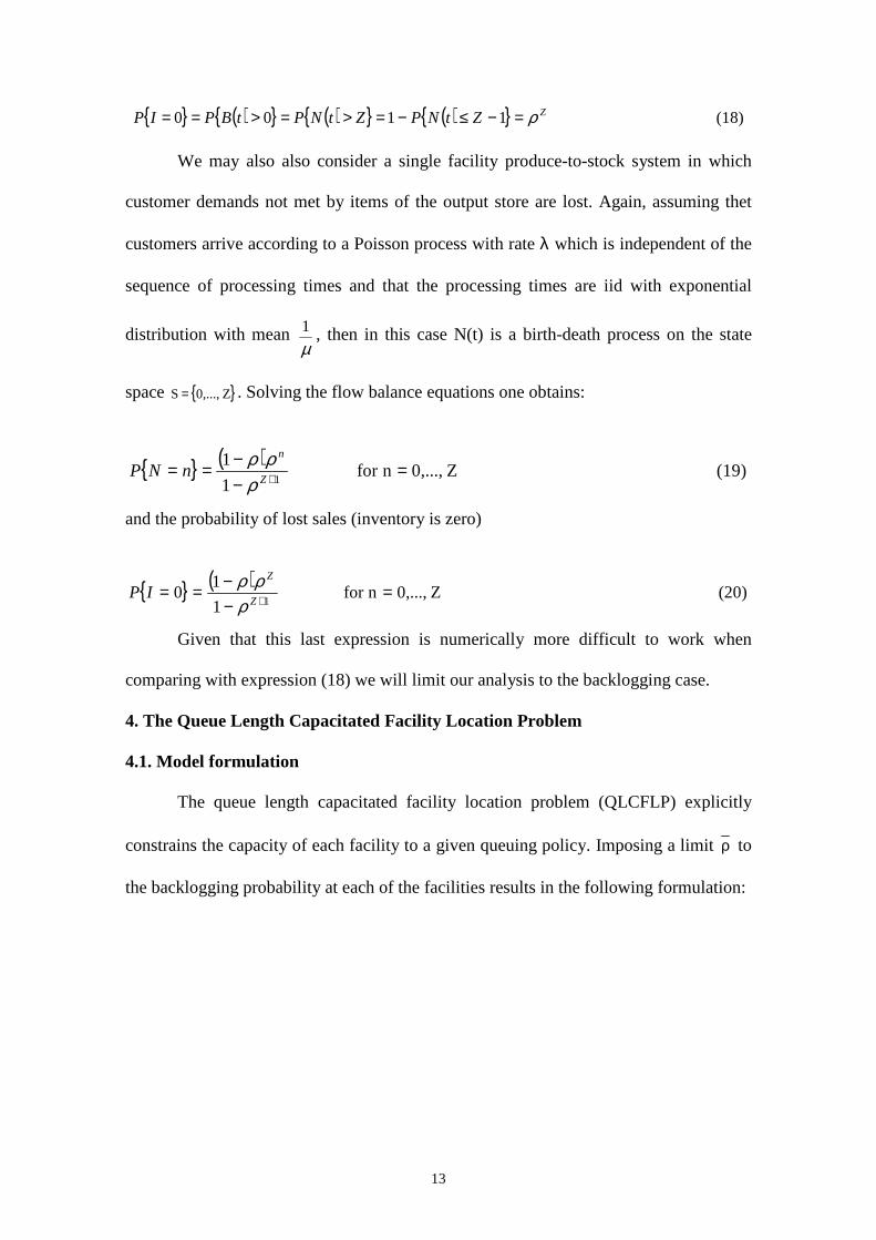
{ } ( ){ } ( ){ } ( ){ } (18) 1100 ZZtNPZtNPtBPIP ρ=−≤−=>=>== We may also also consider a single facility produce-to-stock system in which

customer demands not met by items of the output store are lost. Again, assuming thet

customers arrive according to a Poisson process with rate λ which is independent of the

sequence of processing times and that the processing times are iid with exponential

distribution with mean µ1 , then in this case N(t) is a birth-death process on the state

space { }Z,...,0S= . Solving the flow balance equations one obtains:

{ } ( )(19) Z0,...,nfor

1

11

=−−== +Z

n

nNPρ

ρρ

and the probability of lost sales (inventory is zero)

{ } ( )(20) Z0,...,nfor

1

10

1=

−−== +Z

Z

IPρ

ρρ

Given that this last expression is numerically more difficult to work when

comparing with expression (18) we will limit our analysis to the backlogging case.

4. The Queue Length Capacitated Facility Location Problem 4.1. Model formulation The queue length capacitated facility location problem (QLCFLP) explicitly

constrains the capacity of each facility to a given queuing policy. Imposing a limit ρ to

the backlogging probability at each of the facilities results in the following formulation:

14

{ }{ } (26) j 1,0Y

(25) ji, 1,0X

(24) ji, 0

(23) i 1

(22) j

..

(21) min

j

ij

1

j

m

1i 11

∀∈

∀∀∈

∀∀≤−

∀=

∀≤

+

∑

∑ ∑∑

=

= ==

jij

m

jij

Z

m

jjj

n

jijij

YX

X

ts

YfXC

ρρ

where,

(27) µ

Xfreq

ρ

m

1iiji

j

∑==

is the utilization factor.

Backlogging may be defined as the number of customers in a queue waiting for

the product or service. Imposing a limit to the backlogging probability is equivalent to

restricting the demand assigned to each facility.

The arrival rate at a facility site j is defined as the sum of the frequencies

of all demand points assigned to this facility. µ is the service rate. In order to have a

stationary system one should add the restriction that the service rate is large enough to

cover the arrival rate, i.e.

(28) 1 µ

Xfreq

ρ

m

1iiji

j <=∑

=

Using definition (28) expression (22) can be rewritten as

15

(29) 1

Zn

iiji Xf ρµ≤∑

=

which is linear on the decision variables. For a given limit ρ and for a given service rate

µ the capacities are defined by Z, the maximum number of items that can be reached.

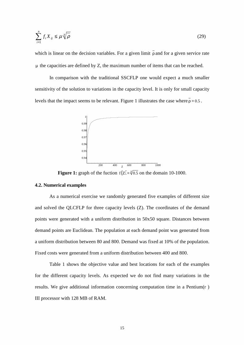
In comparison with the traditional SSCFLP one would expect a much smaller

sensitivity of the solution to variations in the capacity level. It is only for small capacity

levels that the impact seems to be relevant. Figure 1 illustrates the case where 5.0=ρ .

0.94

0.95

0.96

0.97

0.98

0.99

1

200 400 600 800 1000Z Figure 1: graph of the fuction ( ) Z 5.0 Zf = on the domain 10-1000.

4.2. Numerical examples

As a numerical exercise we randomly generated five examples of different size

and solved the QLCFLP for three capacity levels (Z). The coordinates of the demand

points were generated with a uniform distribution in 50x50 square. Distances between

demand points are Euclidean. The population at each demand point was generated from

a uniform distribution between 80 and 800. Demand was fixed at 10% of the population.

Fixed costs were generated from a uniform distribution between 400 and 800.

Table 1 shows the objective value and best locations for each of the examples

for the different capacity levels. As expected we do not find many variations in the

results. We give additional information concerning computation time in a Pentium(r )

III processor with 128 MB of RAM.

16

Table 1 : some numerical results for the QLCFLP

Z=500

Z=1000

Z=5000

NL x ND Objective Locations CPU time Objective Locations CPU time Objective Locations CPU time 30 x 30

1389.35

1;7

02m52s

1389.35

1;7

02m50s

1389.35

1;7

02m52s

40 x 40 1494.62 10;27 04m46s 1494.62 10;27 04m37s 1494.62 10;27 04m30s 45 x 45 1524.44 31;40 02m00s 1524.44 31;40 01m43s 1524.44 31;40 02m32s 50 x 50 1963.77 28;30;46 33m48s 1962.61 28;30;46 21m28s 1962.61 28;30;46 49m17s 60 x 60 1983.26 28;39;47 40m15s 1983.26 28;39;47 19m19s 1982.92 28;39;47 20m07s NL : number of potential locations ND : number of demand nodes 5. A Heuristic algorithm to solve the QLCFLP 5.1. Review of Literature The SSCFLP is a combinatorial optimization problem that belongs to the class

of NP-hard problems. The traditional approach for solving this problem focuses on

obtaining good Lagrangean duals, whose solutions improve the lower bounds provided

by LP relaxation. Both capacity and demand constraints have been relaxed, obtaining in

the first case uncapacitated facility location subproblems and in the second a number of

knapsack problems. Some of those Lagrangean Relaxations can be found in (Barceló et

al. 1984, Beasley 1988 or Barceló et al. 1991).

As suggested by Krarup and Pruzan (1983) the FLP is a “hard nut to crack, or, to

use a more precise characterization, that it is highly unlikely that an exact polynomial

time bounded algorithm can ever be devised for its solution”. These same authors

carachterize the problem in terms of computational complexity, to demonstrate that

indeed it belongs to the class of combinatorial optimization problems termed NP-hard.

Several heuristics have been developed for the CFLP. Jacobsen (Jacobsen 1983)

generalizes heuristics for the Uncapacitated Plant Location Problem to the capacitated

case. The heuristics are ADD, DROP, SHIFT, ALA (alternative location-allocation) and

VSM (vertex substituting method). The ADD and DROP procedures are greedy

heuristics, where in the first case a facility is added at each of the iterations and in the

17

second case a facility is dropped. The chosen facility is always the one where the largest

saving on costs is obtained. Both methods are considered construction methods since no

revision on early decisions is allowed. More sophisticated heuristics are based on the

idea of improving on a known solution. A good example is the Teitz and Bart ( Teitz et

al.1968) Vertex Substitution Method.

Cornuejols (Cornuejols et al. 1991) compare several relaxations for the CFLP

with classical greedy or interchange heuristics. The authors compute various lower

bounds on the objective value relaxing subsets of constraints either completely or in a

Lagrangean fashion. The subsets of constraints considered are: demand constraints,

capacity constraints, non-negativity and integrality constraints. Based on their

experiments the authors suggest the use of a Lagrangean heuristic to solve large

instances of CFLP.

Beasley (Beasley 1993) presents a framework for developing Lagrangean

heuristics with respect to the location problems: p-median, uncapacitated warehouse

location and capacitated warehouse location with or without single source constraints.

The author concludes that the heuristics presented in the paper for the four location

problems is able to generate optimal or near optimal solutions at reasonable computing

cost.

Concerning the SSCFLP, (Delmaire et al. 1999), propose a Reactive GRASP

heuristic, a Tabu Search Heuristic, and two different hybrid approaches that combine

elements of the GRASP and the Tabu Search methodologies.

Holmberg (Holmberg et al. 1999) propose an exact algorithm for the

capacitated facility location problem with single sourcing. Their procedure is based on

Lagrangian heuristics using subgradient optimization. The authors combine a strong

18

dual approach (the Lagrangian dual) with a strong primal (the repeated matching

heuristic).

Cortinhal and Captivo (Cortinhal et al. 2003) use a Lagrangean relaxation to

obtain lower bounds for the SSCPLP, and Lagrangean heuristics followed by search

methods and one Tabu Search metaheuristic to obtain upper bounds. The same authors,

(Cortinhal et al. 2004), use genetic algorithms to solve the SSCPLP.

5.2. Heuristics Solving the CPLP comprises two sub-problems: finding the optimal location of

the facilities and the assignation of demand points to each one of the open facilities. In

fact, for any vector Y of location variables the optimal solution for the flow variables

( )YX can be retrieved by solving the associated transportation problem:

( )

{ } (34) j i, X

(33) j i, YX

(32) i X

(31) j

ts

(30) XCY Zmin

ij

jij

m

jij

Zj

m

1i

n

jijij

∀∀∈

∀∀≤−

∀=

∀≤

=

∑

∑∑

=

= =

1,0

0

1

..

1

1

ρρ

In the heuristic procedure we used a Reactive-GRASP algorithm and two

different types of neighbourhood search: shift neighbourhood and swap neighbourhood.

Reactive GRASP, proposed by Prais and Ribeiro (Prais et al. 2000), is a

procedure in which the parameter is self-adjusted according to the quality of the

solutions previously found. Instead of fixing the value of the parameter γ , which

determines which elements will be placed in the restricted candidate list, R-GRASP

19

randomly selects this parameter value from a discrete set { }m1,...,γγ . The probability

distribution used in the γ selection will be updated after the execution of each block of

iterations considering the quality of the solutions obtained by each of the γi.

Let ϕ be the greedy function for a minimization problem. The Restricted

Candidate List (RCL) contains all the candidate solutions within a given distance of the

top candidate as a function of ϕ. The threshold value can be expressed as:

( ) minmax ϕϕγ −

The Reactive GRASP selects the best value of γ, by measuring the goodness of

each possible value γ and defining an automated selection criterion for this parameter’s

value at the different iterations of the process.

The algorithm we used to solve our problem comprises the following steps:

1- Set initial probabilities v

1Pi = with i=1,...,v. Pi is the probability of choosing a given

parameter iγ=γ . V is the number of candidates for γ. In our particular case we

considered v=10 and a set of candidates { }1 , ... , 1.0

2- For each of the blocks of iterations k=1,...,num_blocks, repeat the following steps:

2.1- For a given number of iterations r=1,...,num_iterations repeat:

2.1.1- Randomly select iγ=γ from { }v1,...,γγ using probabilities iP with i=1,...,v.

2.1.2- Construction phase: construct a greedy randomized solution, considering the

selected value of γ .

2.1.4- Apply local search.

2.2.- Update γ ’s utility ( )γut . We considered the utility of γ as given by the average

deviation of the objectives found using this particular γ from the best value for the

objective found so far.

20

2.3. Compute new probabilities Pi using the following expression: ( )

( )∑=

=v

1

ii

utP

jjut γ

γ

2.4. Go back to step 2.1 and start a new block of iterations.

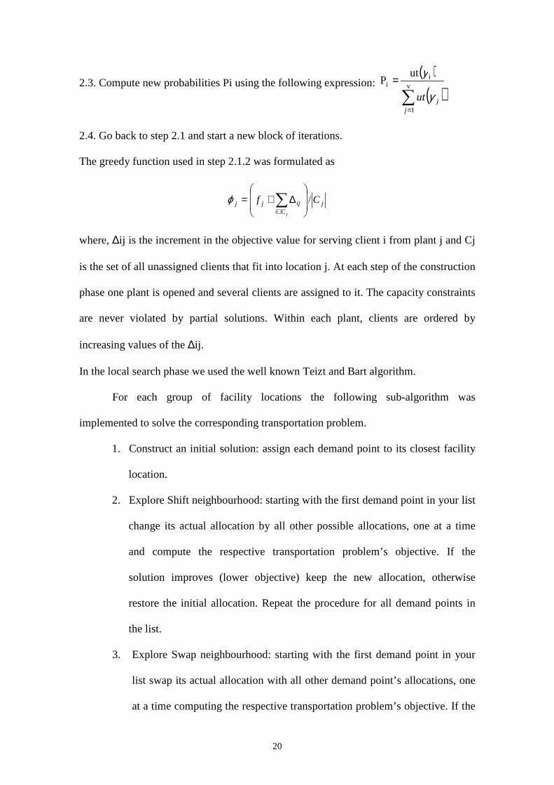
The greedy function used in step 2.1.2 was formulated as

jCi

ijjj Cfj

/

∆+= ∑

∈

ϕ

where, ∆ij is the increment in the objective value for serving client i from plant j and Cj

is the set of all unassigned clients that fit into location j. At each step of the construction

phase one plant is opened and several clients are assigned to it. The capacity constraints

are never violated by partial solutions. Within each plant, clients are ordered by

increasing values of the ∆ij.

In the local search phase we used the well known Teizt and Bart algorithm.

For each group of facility locations the following sub-algorithm was

implemented to solve the corresponding transportation problem.

1. Construct an initial solution: assign each demand point to its closest facility

location.

2. Explore Shift neighbourhood: starting with the first demand point in your list

change its actual allocation by all other possible allocations, one at a time

and compute the respective transportation problem’s objective. If the

solution improves (lower objective) keep the new allocation, otherwise

restore the initial allocation. Repeat the procedure for all demand points in

the list.

3. Explore Swap neighbourhood: starting with the first demand point in your

list swap its actual allocation with all other demand point’s allocations, one

at a time computing the respective transportation problem’s objective. If the

21

solution improves (lower objective) keep the new allocations, otherwise

restore the initial allocations. Repeat the procedure for all demand points in

the list.

We explore both neighbourhoods for all demand points and repeat the searching

process while there are improvements to the solution.

In the Capacitated Facility Location Problem there is no a priori information

about the number of facilities to be located. In our algorithm we started with one facility

and applied an algorithm, which increases the number of facilities by one unit at each

block of iterations. The algorithm stops when there are no improvements in the

objective by locating one extra facility.

Some other authors apply a neighbourhood search, which allows opening or

closing facilities; see as an example (Delmaire et al. 1999).

5.3. Numerical examples

In order to evaluate the heuristics we randomly generated 30 examples using the

same procedure described in section 4.2. Each of the examples was solved for the

optimal using the LINGO commercial package and the heuristics described in the

previous points. Table 2 shows the results regarding the experiments.

As shown in table 2, the results are quite close: from the twenty examples we

didn’t reach the minimum objective in five of the examples. The heuristics allow some

important savings in computing times even for small examples.

22

Table 2: Heuristics statistics.

LINGO HEURISTICS (10 bocks 10 iter) Objective Locations CPU time Objective Locations CPU time EXAMPLE (sec) (sec)

1 1275,64 5;28 127,2 1275,64 5;28 26,42 2 1376,32 3;11 154,8 1376,32 3;11 29,01 3 1308,87 5;24 139,2 1308,87 5;24 24,66 4 1244,58 7;12 70,8 1244,58 7;12 44,71 5 1439,62 7;30 138,6 1439,62 7;30 22,85 6 1395,58 2;24 137,4 1395,58 2;24 63,55 7 1338,24 8;10 136,8 1338,24 8;10 64,76 8 1313,01 19;25 83,4 1351,75 -- 29,01 9 1324,72 7;22 144,6 1325,59 -- -- 10 1336,51 29;30 133,2 1386,94 -- -- 11 1409,55 1;8 264 1409,55 1;8 33,59 12 1275,83 4;22 126 1290,56 -- -- 13 1298,87 10;25 183,6 1298,87 10;25 61,96 14 1287,75 19;29 252,6 1287,75 19;29 23,13 15 1243,1 13;22 210 1243,1 13;22 24,33 16 1279,65 2;11 190,2 1279,65 2;11 21,2 17 1370,32 8;28 154,2 1370,32 8;28 44,87 18 1363,04 6;21 187,2 1363,04 6;21 39,22 19 1279 6;28 211,8 1279 6;28 38,45 20 1250,29 20;26 191,4 1250,29 20;26 24,17 21 1355,67 7;30 82,8 1355,67 7;30 44,05 22 1270,33 24;28 144 1270,33 24;28 24,88 23 1234,12 18;27 244,8 1234,12 18;27 24,39 24 1336,9 2;26 129 1336,9 2;26 33,06 25 1354,75 16;20 249 1354,75 16;20 23,73 26 1302,29 16;30 191,4 1302,29 16;30 26,64 27 1260,3 4;15 144,6 1292,43 -- -- 28 1296,69 7;23 154,2 1296,69 7;23 22,58 29 1247,54 3;7 73,2 1247,54 3;7 34 30 1254,24 15;19 144,6 1254,24 15;19 24,33

Number of distinct solutions (%)

16%

Average deviation (%) 0.34% Maximum deviation (%) 4%

Average CPU time – LINGO 259.82 s Average CPU time – Heuristics 33.59 s

23

6. A simulation exercise Since stochastic systems in general are easy to simulate and an objective

function can be computed for each of the simulated scenarios, simulation can be

combined with optimization algorithms in order to optimize many real life problems.

For a good presentation of the role of simulation in optimization techniques, refer to the

textbook by (Gasovi 2003).

One of the assumptions of the model formulated in previous sections consists of

observing a stochastic demand whose arrival rate follows a Poisson distribution. A

simple exercise developed in this section consists of simulating one arrival process at

each one of the demand points for one hundred simulations. Then, we solved the

QLCFLP and check if the solution changes at each one of the simulations. We used the

heuristic described in the previous section to solve each of the problems.

Across the different examples we maintain the distance matrix, as well as the

location of the demand points. The only parameter changing is the arrival rate at each of

the demand points. These rates were simulated from a Poisson distribution with a

specific parameter (average) for each demand point. For simplicity only we considered

twenty demand points. The average arrival rate at each of the demand points is shown in

the following table:

Table 3: A Simulation Exercise: Average arrival rate.

i 1 2 3 4 5 6 7 8 9 10 11 12 13 14 15 16 17 18 19 20

λ 72 40 30 68 19 24 15 75 48 71 47 25 72 56 77 37 66 50 78 47

If we consider, as an example a service rate of two hundred (µ = 200) and a

maximum of two hundred tags available ( Z = 200), the left hand side of equation ….

for different capacity levels, measured in terms of utilization ratio ( ρ ) are the ones in

table 4:

24

Table 4: A Simulation Exercise: Capacities.

We run the simulations for the extreme cases and compare the objectives for the

extreme cases, where ρ =0,1 and ρ =0,9. The results are shown in figure 2a) and in

figures 2b) respectively.

820

840

860

880

900

920

940

Figure 2a): Objective values : ρ =0,9

.

ρ LHS 0,1 197,7106 0,2 198,397 0,3 198,7996 0,4 199,0858 0,5 199,3081 0,6 199,4898 0,7 199,6436 0,8 199,777 0,9 199,8947

Average Objective 870,5968 Standard Deviation 11,20544

25

820

840

860

880

900

920

940

Figure 2b): Objective values : ρ =0,1

The resulting graphs suggest that in spite of in some exceptional cases the objectives

may be different; the average objective is quite similar when we change the upper limit

for the utilization ratio. The standard deviations in both cases are relatively low.

7. Conclusions

This paper considers a new formulation for the Single Source Capacitated Facility

Location Problem in which capacity constraints result from imposing an upper bound to

the probability of customers’ demand being backlogged. Demand is assumed to be

stochastic, following a Poisson distribution and coincides with the arrival rate of a

Markovian M/M/1 queuing process.

Theory on stochastic manufacturing systems as well as some numerical examples

suggests that solutions in this new model become less sensitive to variations in

capacities.

Average Objective 870,7439 Standard Deviation 8,857857

26

Knowing the probability distribution of the demand, it is possible to simulate

demand. Some simulated examples show that the results do not vary much across the

different scenarios.

Finally, greedy heuristics seems to behave well when solving this new

formulation of the Single Source Capacitated Facility Location Problem.

27

References

Balinski, M. L. Integer Programming: Methods, uses, computations. Management

Science,1965, 12, 253-313.

Balinski, M. L. On finding integer solutions to linear programs. Proc. IBM Scientific

Symposium on Combinatorial Problems, 1966. 225-248.

Balinski, M. L. and K. Spielberg. Methods for integer programming: algebraic,

combinatorial, and enumerative. Progress in Operations Research, 1969. 195-292.

Barceló, J. and J. Casanovas. A heuristis algorithm for the Capacitaed Plant Location

Problem European Journal of Operational Research, 1984, 15(2),212-226.

Barceló, J. E. Fernandéz and K. Jörnsten. Computational results from a new Lagrangean

Relaxation algorithm for the Capacitated Plant Location Problem. European Journal

of Operational Research,1991, 53, 38-45.

Beasley, J. E.. An algorithm for solving large capacitated warehouse location problems.

European Journal of Operational Research , 1988, 33, 314-325.

Beasley, J. E. Lagrangean heuristics for location problems. European Journal of

Operational Research, 1993, 65, 383-399.

Buzacott, J. and J. Shanthikumar. Stochastic Models of Manufacturing Systems.

Prentice Hall Publishers. 1993.

Cornuejols, G., R. Sridharan and J.M. Thizy. A comparison of heuristics and relaxations

for the Capacitated Plant Location Problem. European Journal of Operational

Research, 1991, 50, 280-297.

Cornuejols, G. Analysis of algorithms for a class of location problems. Technical

Report no. 382, SORIE, Cornell University.

28

Cortinhal, J. and M. E. Captivo. Upper and lower bounds for the single source

capacitated location problem. European Journal of Operational Research, 2003, 151,

333-351.

Cortinhal, J. and M. E. Captivo.Genetic algorithms for the single source capacitated

location problem. in Metaheuristics Computer Decision-Making. Edited by Mauricio

Resende e Jorge Pinho de Sousa. Kluwer Academic Publishers.2004. pp 187-216.

Delmaire, H., J. A. Díaz and E. Fernández. Reactive GRASP and Tabu search based

heuristics for the Single Source Capacitated Plant Location Problem. INFOR, 1999,

37, no. 3.

Gasovi, A. Simulation-based optimization: an overview. Kluwer Academic

Publishers.2003.

Guignard, M. and K. Spielberg. Algorithms for exploiting the structure of the simple

plant location problem. Annals of Discrete Math, 1977. 1, 247-228.

Holmberg, K. Exact solution methods for uncapacitated location problems with convex

transportation costs. European Journal of Operational Research, 1999, 114. 127-

140.

Jacobsen, S. K. Heuristics for the capacitated plant location model. European Journal of

Operational Research, 1983, 12, 253-261.

Krarup, J. and M. Pruzan. The simple plant location problem: Survey and synthesis.

European Journal of Operational Research, 1983, 12. 36-81.

Kuehn, A.A. and M.J. Hamburger. A heuristic program for locating warehouses.

Management Science, 1963, 9, 643-666.

Manne, A. S. Plant location under economies-of-scale- decentralization and

computation. Management Science, 1964, 11, 213-235.

29

Prais, M. and C.C. Ribeiro. Reactive GRASP an application to a Matrix Decomposition

Problem in TDMA traffic assignment. INFORMS Journal on Computing, 2000,12,

vol.3.

ReVelle, C.S., D. Marks and J.C. Liebman. An analysis of private and public sector

location models. Management Science, 1970. 16, 692-707.

Rönnqvist, M., S. Tragantalerngsak and J, Holt. A repeated matching heuristic for the

single-source capacitated facility location problem. European Journal of Operational

Research, 1999, 116, 51-68.

Suri, R., J. Sanders and M. Kamath. Performance Evaluation of Production Networks

in Logistics of Production and Inventory edited by S. Graves, A. Kan and P. Zipkin.

Elsevier Science Publishers, 1993, 199-274.

Sridharan R. The capacitated plant location problem. European Journal of Operational

Research, 1995, 87, 203-213.

Stecke, K. and J. Aronson. Review of operator/machine interference models.

International Journal of Production Research, 1985, 23, 129-151.

Teizt, M.B. and Bart, P. Heuristic methods for estimating the generalized vertex median

of weighted graph. Operations Research, 1968, 16(5), 955-961.

30

Acknowledgments

This research has been possible thanks to the grant SFRH/BD/2916/2000 from the

Ministério da Ciência e da Tecnologia, Fundação para a Ciência e a Tecnologia of the

Portuguese government., and grant SEC2003-1991 from the Ministry of Education and

Science, Spain.