a case of depth-3 identity testing, sparse factorization and duality

comput. complex. 22 (2013), 39 – 69

c© Springer Basel 2012

1016-3328/13/010039-31

published online December 15, 2012

DOI 10.1007/s00037-012–0054-4 computational complexity

A CASE OF DEPTH-3 IDENTITY

TESTING, SPARSE

FACTORIZATION AND DUALITY

Chandan Saha, Ramprasad Saptharishi,

and Nitin Saxena

Abstract. The polynomial identity testing (PIT) problem is known tobe challenging even for constant depth arithmetic circuits. In this work,we study the complexity of two special but natural cases of identitytesting—first is a case of depth-3 PIT, the other of depth-4 PIT.Our first problem is a vast generalization of verifying whether a boundedtop fan-in depth-3 circuit equals a sparse polynomial (given as a sum ofmonomial terms). Formally, given a depth-3 circuit C, having constantmany general product gates and arbitrarily many semidiagonal productgates test whether the output of C is identically zero. A semidiagonalproduct gate in C computes a product of the form m · ∏b

i=1 �eii , where

m is a monomial, �i is a linear polynomial, and b is a constant. Wegive a deterministic polynomial time test, along with the computationof leading monomials of semidiagonal circuits over local rings.The second problem is on verifying a given sparse polynomial factoriza-tion, which is a classical question (von zur Gathen, FOCS 1983): Givenmultivariate sparse polynomials f, g1, . . . , gt explicitly check whetherf =

∏ti=1 gi. For the special case when every gi is a sum of univariate

polynomials, we give a deterministic polynomial time test. We charac-terize the factors of such gi’s and even show how to test the divisibilityof f by the powers of such polynomials.The common tools used are Chinese remaindering and dual represen-tation. The dual representation of polynomials (Saxena, ICALP 2008)is a technique to express a product-of-sums of univariates as a sum-of-products of univariates. We generalize this technique by combining it

40 Saha et al. cc 22 (2013)

with a generalized Chinese remaindering to solve these two problems(over any field).

Keywords. Identity testing, arithmetic circuits, ideals, factorization,Galois rings.

Subject classification. 68W30.

1. Introduction

Polynomial identity testing (PIT) is one of the most fundamen-tal problems of algebraic complexity theory. A central object ofstudy in the subject of algebraic complexity is the arithmetic circuitmodel of computation. Arithmetic circuits, an algebraic analogueof boolean circuits with addition and multiplication gates replacing‘or’ and ‘and’ gates, form a natural and concise way to representpolynomials in many variables. It has always been an interestingand challenging task for the research community to understand thepowers and limits of this model.

Identity testing is an algorithmic problem on arithmetic cir-cuits. It is the task of checking whether the output of a givenarithmetic circuit is zero as a formal polynomial. Interestingly,this natural algebraic problem is deeply connected to fundamen-tal lower bound questions in complexity theory (Agrawal 2005;Kabanets & Impagliazzo 2003) and is also critically used in the de-signing of efficient algorithms for several other important problems(Agrawal et al. 2004; Clausen et al. 1991; Lovasz 1979). Some ofthe other milestone results in complexity theory, like IP = PSPACE(Lund et al. 1990; Shamir 1990) and the PCP theorem (Arora et al.1998) also involve PIT.

Identity testing does admit a randomized polynomial timealgorithm—choose a random point from a sufficiently large fieldand evaluate the circuit (Schwartz 1980; Zippel 1979). With highprobability, the output is nonzero if the circuit computes a nonzeropolynomial. There are several other more efficient randomizedalgorithms (Agrawal & Biswas 1999; Chen & Kao 1997; Klivans& Spielman 2001; Lewin & Vadhan 1998). Refer to the surveyAgrawal & Saptharishi (2009) for a detailed account of them.

cc 22 (2013) Depth-3 PIT, sparse factorization and duality 41

Derandomizing identity testing is important from both thealgorithmic and the lower bound perspectives. For instance, thedeterministic primality test in Agrawal, Kayal & Saxena (2004)involves derandomization of a certain polynomial identity test.On the other hand, it is also known (Agrawal 2005; Kabanets &Impagliazzo 2003) that a certain strong derandomization of PITimplies that the permanent polynomial requires super-polynomial-sized arithmetic circuits (in other words, VP �= VNP).

Derandomizing the general problem of PIT has proven to bea difficult endeavor. Restricting the problem to constant depthcircuits, the first non-trivial case arise for depth-3 circuits. Quitestrikingly, it is now known (Agrawal & Vinay 2008) that depth-4 circuits capture the difficulty of the general problem of PIT: Ablack-box identity test for depth-4 circuits gives a quasi-polynomialtime PIT algorithm for circuits computing low- degree polynomi-als. Another notable result is by Raz (2010), but more in the flavorof lower bounds, shows that strong enough depth-3 circuit lowerbounds imply super-polynomial lower bounds for general arith-metic formulas. Although the general case of depth-3 PIT is stillopen, some special cases like depth-3 circuits with bounded top fan-in (Kayal & Saxena 2007; Saxena & Seshadhri 2011) and diagonaldepth-3 circuits (Saxena 2008) are known to have deterministicpolynomial time solutions. In the depth-4 setting, it is known howto do (black-box) PIT for multilinear circuits with bounded topfan-in (Saraf & Volkovich 2011) also in polynomial time. Refer tothe surveys Saxena (2009) and Shpilka & Yehudayoff (2010) fordetails on results concerning depth-3 and depth-4 PIT (and muchmore).

1.1. The motivation. The motivation behind our work is aquestion on ‘composition of identity tests’. Suppose we know howto perform identity tests efficiently on two classes of circuits A andB. How easy is it to solve PIT on the class of circuits A + B?The class A + B is made up of circuits C of the form C1 + C2,where C1 ∈ A and C2 ∈ B. In other words, the root node of Cis an addition gate with the roots of C1 and C2 as its children.(Notice that, PIT on the class C1 × C2 is trivial.) Dependingon the classes A and B, this question can be quite non-trivial to

42 Saha et al. cc 22 (2013)

answer. For instance, suppose we are given t + 1 sparse polyno-mials f, g1, . . . , gt, explicitly as sums of monomials, and asked tocheck whether f =

∏ti=1 gi. Surely, it is easy to check whether

f or∏t

i=1 gi is zero. But, it is not clear how to perform the test

f − ∏ti=1 gi

?= 0. (This problem has also been declared open in a

work by von zur Gathen (1983) on sparse multivariate polynomial

factoring.) The test f − ∏ti=1 gi

?= 0 is one of the most basic cases

of depth-4 PIT that is still open. Annoyingly enough, it showsthat while PIT on depth-3 circuits with top fan-in 2 is trivial, PITon depth-4 circuits with top fan-in 2 is far from trivial.

We wonder what can be said about composition of subclassesof depth-3 circuits. Two of the non-trivial classes of depth-3 cir-cuits for which efficient PIT algorithms are known are the classesof bounded top fan-in (Kayal & Saxena 2007) and diagonal (orsemidiagonal) circuits (Saxena 2008). The question is—Is it pos-sible to glue together the seemingly disparate methods of Kayal& Saxena (2007) and Saxena (2008) and give a PIT algorithmfor the composition of bounded top fan-in and semidiagonal cir-cuits? In this work, we answer this question in the affirmative.Our technique also applies to a special case of the depth-4 prob-

lem: f − ∏ti=1 gi

?= 0.

1.2. Our contribution. We give deterministic polynomial timealgorithms for two problems on identity testing—one is on a classof depth-3 circuits, while the other is on a class of depth-4 circuits.As mentioned in Section 1.1, both these classes can be viewed ascomposition of subclasses of circuits over which we already knowhow to perform PIT.

Our first problem is a common generalization of the problemsstudied in Kayal & Saxena (2007) and Saxena (2008). We needthe following definition of a semidiagonal circuit.

Definition 1.1. (Semidiagonal circuit) Let C be a depth-3 circuit,that is, a sum of products of linear polynomials. The top fan-inof C is the number of such product gates. If each product gate inC computes a polynomial of the form m · ∏b

i=1 �eii , where m is a


monomial, �i is a linear polynomial in the n input variables and bis a constant, then C is a semidiagonal circuit.

Remark. Our results hold even with the relaxed definition ofsemidiagonal circuits where b is not necessarily a constant but∏b

i=1 (1+ei) ≤ poly(size(C)). For this, we need a slightly tighteranalysis for dual representation in Section 2(refer to Saxena (2008)).This gets interesting when all eis are O(1) as our test could thenafford up to b = O(log size(C)).

Problem 1. Given a depth-3 circuit C1 with bounded top fan-inand given a semidiagonal circuit C2, test whether the output of thecircuit C1 + C2 is identically zero.

Our second problem is a special case of checking a given sparsemultivariate polynomial factorization (thus, a case of depth-4 topfan-in 2 PIT).

Problem 2. Given t+1 polynomials f, g1, . . . , gt explicitly as sumof monomials, where every gi is a sum of univariate polynomials,check whether f =

∏ti=1 gi.

It is possible that though f is sparse, some of its factors are notsparse (an example is provided in Section 5). So, multiplying thegis in a brute force fashion is not a feasible option. In this paper,we show the following:

Theorem 1.2. Problem 1 and Problem 2 can be solved in deter-ministic polynomial time.

The asymptotics of Theorem 1.2 appear at the end of Section 4and Section 5.

1.3. An overview of our approach. Our first common tool insolving both Problem 1 and Problem 2 is called the dual represen-tation of polynomials (Saxena 2008). It is a technique to expressa power of a sum of univariates as a ‘small’ sum of product of uni-variates. In the latter representation, we show how to efficientlycompute the leading monomial (and its coefficient), under the nat-ural lexicographic ordering (Section 3). This observation turns out

44 Saha et al. cc 22 (2013)

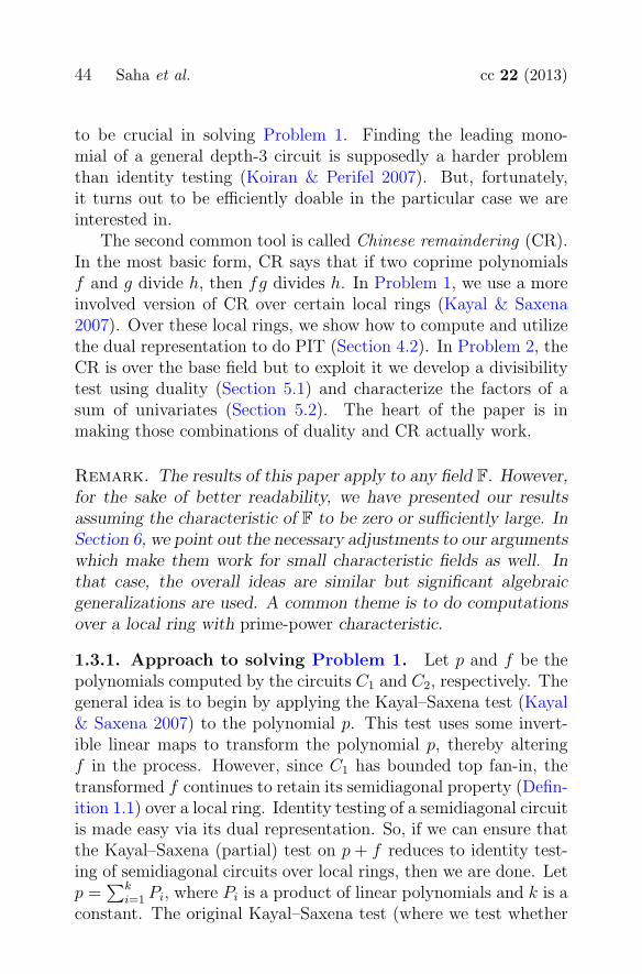
to be crucial in solving Problem 1. Finding the leading mono-mial of a general depth-3 circuit is supposedly a harder problemthan identity testing (Koiran & Perifel 2007). But, fortunately,it turns out to be efficiently doable in the particular case we areinterested in.

The second common tool is called Chinese remaindering (CR).In the most basic form, CR says that if two coprime polynomialsf and g divide h, then fg divides h. In Problem 1, we use a moreinvolved version of CR over certain local rings (Kayal & Saxena2007). Over these local rings, we show how to compute and utilizethe dual representation to do PIT (Section 4.2). In Problem 2, theCR is over the base field but to exploit it we develop a divisibilitytest using duality (Section 5.1) and characterize the factors of asum of univariates (Section 5.2). The heart of the paper is inmaking those combinations of duality and CR actually work.

Remark. The results of this paper apply to any field F. However,for the sake of better readability, we have presented our resultsassuming the characteristic of F to be zero or sufficiently large. InSection 6, we point out the necessary adjustments to our argumentswhich make them work for small characteristic fields as well. Inthat case, the overall ideas are similar but significant algebraicgeneralizations are used. A common theme is to do computationsover a local ring with prime-power characteristic.

1.3.1. Approach to solving Problem 1. Let p and f be thepolynomials computed by the circuits C1 and C2, respectively. Thegeneral idea is to begin by applying the Kayal–Saxena test (Kayal& Saxena 2007) to the polynomial p. This test uses some invert-ible linear maps to transform the polynomial p, thereby alteringf in the process. However, since C1 has bounded top fan-in, thetransformed f continues to retain its semidiagonal property (Defin-ition 1.1) over a local ring. Identity testing of a semidiagonal circuitis made easy via its dual representation. So, if we can ensure thatthe Kayal–Saxena (partial) test on p + f reduces to identity test-ing of semidiagonal circuits over local rings, then we are done. Letp =

∑ki=1 Pi, where Pi is a product of linear polynomials and k is a

constant. The original Kayal–Saxena test (where we test whether


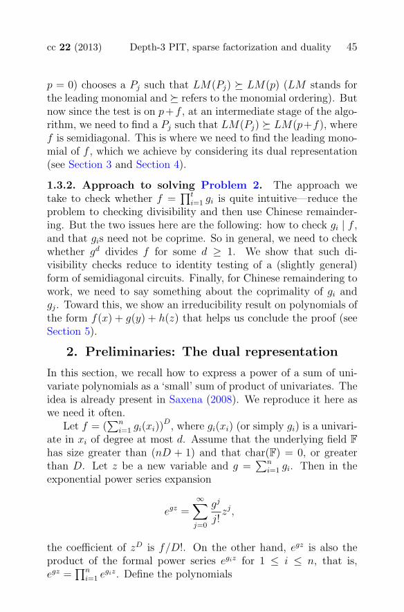
p = 0) chooses a Pj such that LM(Pj) � LM(p) (LM stands forthe leading monomial and � refers to the monomial ordering). Butnow since the test is on p+f , at an intermediate stage of the algo-rithm, we need to find a Pj such that LM(Pj) � LM(p+f), wheref is semidiagonal. This is where we need to find the leading mono-mial of f , which we achieve by considering its dual representation(see Section 3 and Section 4).

1.3.2. Approach to solving Problem 2. The approach wetake to check whether f =

∏ti=1 gi is quite intuitive—reduce the

problem to checking divisibility and then use Chinese remainder-ing. But the two issues here are the following: how to check gi | f ,and that gis need not be coprime. So in general, we need to checkwhether gd divides f for some d ≥ 1. We show that such di-visibility checks reduce to identity testing of a (slightly general)form of semidiagonal circuits. Finally, for Chinese remaindering towork, we need to say something about the coprimality of gi andgj. Toward this, we show an irreducibility result on polynomials ofthe form f(x) + g(y) + h(z) that helps us conclude the proof (seeSection 5).

2. Preliminaries: The dual representation

In this section, we recall how to express a power of a sum of uni-variate polynomials as a ‘small’ sum of product of univariates. Theidea is already present in Saxena (2008). We reproduce it here aswe need it often.

Let f = (∑n

i=1 gi(xi))D, where gi(xi) (or simply gi) is a univari-

ate in xi of degree at most d. Assume that the underlying field F

has size greater than (nD + 1) and that char(F) = 0, or greaterthan D. Let z be a new variable and g =

∑ni=1 gi. Then in the

exponential power series expansion

egz =∞∑

j=0

gj

j!zj,

the coefficient of zD is f/D!. On the other hand, egz is also theproduct of the formal power series egiz for 1 ≤ i ≤ n, that is,egz =

∏ni=1 egiz. Define the polynomials

46 Saha et al. cc 22 (2013)

ED(gi, z) =D∑

j=0

gij

j!zj.

Then, the coefficient of zD in the formal power series∑∞

j=0gj

j!zj is

exactly equal to the coefficient of zD in the polynomial P (z) :=∏ni=1 ED(gi, z). The idea is to use interpolation to express this

coefficient of zD as an F-linear combination of few evaluations ofP (z) at different field points.

Suppose P (z) =∑nD

j=0 pjzj, where pjs are polynomials in the

variables x1, . . . , xn. Choose (nD + 1) distinct points α0, . . . , αnD

from the field F and let V be the (nD+1)×(nD+1) Vandermondematrix (αk

j )0≤j,k≤nD. Then,

V · (p0, . . . , pnD)T = (P (α0), . . . , P (αnD))T ,

which implies (p0, . . . , pnD)T = V−1 · (P (α0), . . . , P (αnD))T .

In other words, pD can be expressed as an F-linear combination ofthe P (αj)’s for 0 ≤ j ≤ nD. Now, to complete the sketch, noticethat pD = f/D! and each P (αj) is a product of the univariatesED(gi, αj) of degree (in xi) at most dD. This proves the followingtheorem.

Theorem 2.1. (Saxena 2008) Given f = (∑n

i=1 gi(xi))D, where

gi is a univariate in xi of degree at most d, f can be expressedas a sum of (nD + 1) products of univariates of degree dD, inpoly(n, d,D) time.

3. Finding the leading monomialof semidiagonal circuits

In this section, we present an efficient algorithm to compute theleading monomial of a semidiagonal circuit f . This will be crucialin both the problems that we later solve.

Definition 3.1. (Monomial and coefficient) Let m be a monomialand f a polynomial in the variables x1, . . . , xn. Fix a monomialordering � by x1 � · · · � xn. LM(f) denotes the leading mono-mial in f (conventionally, LM(0) := ∅ and we define xi � ∅, for alli). We denote the coefficient of m in f by [m]f .


We remark that given a semidiagonal circuit f finding LM(f)is indeed a non-trivial problem since the leading monomials gen-erated by the product terms m · ∏b

i=1 �eii in f might cancel off in

such a way that LM(f) is strictly smaller than any of the leadingmonomials of the terms m · ∏b

i=1 �eii . Using Theorem 2.1 and by

the definition of semidiagonal circuits, it is sufficient to present analgorithm for finding the leading monomial of a sum of productof univariates. Our argument is similar in spirit to that of thenon-commutative formula identity test of Raz & Shpilka (2004)but with the added feature that it also finds the coefficient of theleading monomial, which is supposedly a harder problem in thegeneral case.

Theorem 3.2. Given f =∑k

i=1

∏nj=1 gij(xj) over a field F, where

gij is a univariate in xj of degree at most d, the leading monomialof f (and its coefficient) can be found in poly(nkd) time.

Proof. The following discussion gives an efficient iterative al-gorithm to find both LM(f) and [LM(f)]f .

In general, at the �th iteration, we would need to find the lead-ing monomial of a polynomial of the form

f� =k∑

i=1

Gi,�−1 ·n∏

j=�

gij,

where Gi,�−1s are polynomials in x1, . . . , x�−1 and LM(f)=LM(f�).To begin, � = 1 and Gi0 = 1 for all 1 ≤ i ≤ k.

Fix an integer � ∈ [1, n]. Consider the monomials with nonzerocoefficients occurring in the products Gi,�−1 · gi�, for all 1 ≤ i ≤ k.Let the set of these monomials be M� := {m1, . . . ,mμ(�)} suchthat m1 � m2 � · · · � mμ(�). Similarly, consider the monomialswith nonzero coefficients in the partial products

∏nj=�+1 gij for all

1 ≤ i ≤ k and call them N� := {n1, . . . , nν(�)} (also assume thatn1 � n2 � · · · � nν(�)). Then, for any i,

Gi,�−1 · gi� =

μ(�)∑

r=1

cirmr andn∏

j=�+1

gij =

ν(�)∑

s=1

disns,

where the coefficients cir and dis belong to F.

48 Saha et al. cc 22 (2013)

Notice that the monomials mr ·ns are distinct for distinct tuples(r, s). The coefficient of mr · ns in f� is exactly

∑ki=1 cirdis. Put

differently, if cr is the k-dimensional row vector (c1r, . . . , ckr) andds is the row vector (d1s, . . . , dks) then

[mr · ns]f� = cr·dTs .

Consider the μ(�) × k matrix C with vectors cr as rows, for all1 ≤ r ≤ μ(�), and D be the k × ν(�) matrix with vectors dT

s ascolumns, for all 1 ≤ s ≤ ν(�). The coefficient of mr · ns is the(r, s)th entry of the product matrix CD.

We are interested in finding LM(f�). Now notice that the lex-icographically smallest possible index (r, s) for which there is anonzero entry in CD gives the leading monomial mr · ns of f�.This is because of the monomial orderings m1 � m2 � · · · � mμ(�)

and n1 � n2 � · · · � nν(�). Therefore, if there is a row vector cr

in C that is F-linearly dependent on the vectors c1, . . . , cr−1, thenLM(f�) can never be of the form mr · ns for any s, and so we cansafely drop the row cr from C. Since C is a μ(�) × k matrix, thenumber of linearly independent rows of C is at most k. Hence, wecan iteratively drop rows from C that are linearly dependent onprevious rows, until we are left with a new matrix C with at mostk rows.

The dropping of a row cr from C corresponds to pruning themonomial mr from the product Gi,�−1 · gi�. By this, we mean thefollowing. Let M� be the subset of those monomials of M� suchthat mr ∈ M� if and only if cr is a row of C. Let Gi� be theproduct Gi,�−1 · gi� projected to only the monomials in M�, that is,Gi� :=

∑mr∈M�

cirmr. Then, the leading monomial of

f�+1 :=k∑

i=1

Gi� ·n∏

j=�+1

gij

is the same as LM(f�) for the reason explained in the last para-graph. The good part is that M� has at most k monomials andso do the polynomials Gi� for all 1 ≤ i ≤ k. Since the number ofmonomials in Gi� does not grow with �, it is easy to see that bothLM(f) and [LM(f)]f can be found in poly(nkd) time by adaptingthe above discussion into an iterative algorithm. �


Corollary 3.3. Let C be a semidiagonal circuit (Definition 1.1)of top fan-in s and formal degree d. Then, LM(C) and [LM(C)]Ccan be computed in poly(s, (nd)b) time.

Proof. We do this by replacing each power of a linear poly-nomial in the product gates of C by its dual expression given byTheorem 2.1. Next, we partially expand out each product gate tostill get a sum of products of univariates. Per product gate, thiscould blow up the final expression size to at most (nd)O(b). �

4. Solving Problem 1

In Problem 1, suppose p and f be the polynomials computed by C1

and C2, respectively. We need to test whether p + f = 0. Assume,without any loss of generality, that p and f are homogeneous poly-nomials having the same degree d. Let p =

∑ki=1 Pi, where k is

a constant and Pi is a product of d linear forms over F, for all1 ≤ i ≤ k. Let X = {x1, . . . , xn} be the underlying set of vari-ables. Also, suppose s is the number of product gates in C2. Ouralgorithm builds upon Kayal & Saxena (2007), which tests if p = 0.To put things in context, we briefly review their algorithm first.

4.1. Reviewing the Kayal–Saxena test. The algorithm inKayal & Saxena (2007) uses recursion on the top fan-in of C1 tocheck whether p = 0. At an intermediate level of the recursion, thealgorithm finds out if a polynomial of the form

α1T1 + · · · + αk′Tk′

is zero over a local ring R ⊇ F, where k′ ≤ k and αis are elementsof R. Each Ti is a product of linear polynomials over R, where alinear polynomial over R is of the kind

a1xv1 + · · · + an′xvn′ + τ,

where ai ∈ F and τ ∈ M, the unique maximal ideal of R. Inaddition, there is at least one nonzero ai, and xvi

∈ X is a freevariable over R. At the start of the recursion, R = F and M = (0),the null ideal.

50 Saha et al. cc 22 (2013)

The following Algorithm ID takes as input an F-basis of a localring R and checks whether the polynomial

∑k′i=1 αiTi is identically

zero over R and returns YES or NO accordingly. The descriptionof Algorithm ID given below is the same as in Kayal & Saxena(2007), except a slight modification in Step 3.1 which is somewhatnecessary for our purpose (see remark after Algorithm ID).

Algorithm ID(R, 〈α1, . . . , αk′〉, 〈T1, . . . , Tk′〉):

Step 1: (Rearranging terms) Order the terms αiTi so that

LM(T1) � LM(Ti), for all 2 ≤ i ≤ k′. Let p =∑k′

i=1 αiTi.

Step 2: (Base Case) If k′ = 1 check whether α1 = 0. If so, returnYES otherwise NO.

Step 3: (Verifying that p = 0 mod T1) The product T1 can besplit as T1 = S1 . . . Sr, with possible change in the constant α1,such that each Sj is of the form

Sj = (�j + τ1) · (�j + τ2) . . . (�j + τtj),

where τi ∈ M and �j is a linear form over F. Further, for i �= j,�i and �j are coprime linear forms over F. Check whether p =0 mod Sj, for every 1 ≤ j ≤ r. This is done in the following way.

Step 3.1: (Applying a linear transformation) Find a freevariable xu with nonzero coefficient cu in �j. Define aninvertible linear transformation σ on the free variables(occurring in T1, . . . Tk′), sending �j to xu, as follows:σ(xu) = c−1

u (xu − �j + cuxu) and for any other freevariable xv �= xu, σ(xv) = xv.

Step 3.2: (Recursively verify whether σ(p) = 0 mod σ(Sj))Define the ring

R′ = R[xu]/(σ(Sj)),

where xu is the same variable xu in Step 3.1. Noticethat σ(Sj) is of the form

σ(Sj) = (xu + τ1) . . . (xu + τtj),


and σ(T1) = 0 mod σ(Sj). For 2 ≤ i ≤ k′, computeelements βi ∈ R′ and T ′

i such that,

σ(Ti) = βiT′i mod σ(Sj),

where T ′i is a product of linear polynomials over R′.

Recursively call ID(R′, 〈β2, . . . , βk′〉, 〈T ′2, . . . , T

′k′〉). If

the recursive call returns NO, then output NO and exit,otherwise declare p = 0 mod Sj.

Declare p = 0 mod T1, if p = 0 mod Sj for all 1 ≤ j ≤ r.

Step 4: Compute [LM(T1)]p by considering is such that LM(Ti) =LM(T1) and computing the sum (over such is) of αi ·

∏j [LM(�ij)]

�ij, where Ti =∏

j �ij. If [LM(T1)]p = 0, then return YES elseNO.

Remark on Step 3.1. In Kayal & Saxena (2007), the lineartransformation σ is described as a map that takes �j to somefixed variable x1 and transforms the remaining variables x2, . . . , xn

accordingly so that σ is invertible. In our case, we also need theproperty that σ maps only one variable to a general linear form,whereas any other variable is mapped to a variable only. To stressupon this property, we have defined σ in a slightly different way.We will need this attribute of σ, in Section 4.2, to ensure that acertain ‘semidiagonal’ structure of the given sparse polynomial fis preserved at every intermediate stage of the algorithm.

4.1.1. Correctness of Algorithm ID. Suppose Step 3 ensuresthat p = 0 mod T1, where LM(T1) � LM(Ti) for all 2 ≤ i ≤ k′

which also means that LM(T1) � LM(p). The way a linear formis defined over R, it follows that [LM(T1)]T1 is a nonzero fieldelement. Therefore, p = α · T1 for some α ∈ R, implying thatp = 0 if and only if [LM(T1)]p = 0. This is verified in Step 4.

It remains to show the correctness of Step 3. In order to checkwhether p = 0 mod T1, the algorithm finds out if p = 0 mod Sj forevery 1 ≤ j ≤ r. That this is a sufficient condition is implied by thefollowing lemma (also known as ‘Chinese Remaindering over localrings’). The way a local ring R is formed in Algorithm ID it has

52 Saha et al. cc 22 (2013)

the property that every element r ∈ R can be uniquely expressedas r = a + τ , where a ∈ F and τ ∈ M. Let φ be a projection map,taking r to a, that is, φ(r) = a. This map naturally extends topolynomials over R by acting on the coefficients.

Lemma 4.1. (Kayal & Saxena 2007) Let R be a local ring overF and p, g, h ∈ R[x1, . . . , xn] be multivariate polynomials suchthat φ(g) and φ(h) are coprime over F. If p = 0 mod g andp = 0 mod h, then p = 0 mod gh.

Since φ(Sj) = �tjj and �i, �j are coprime for i �= j, the correctness

of Step 3 follows. Finally, notice that, p = 0 mod Sj if and onlyif σ(p) = 0 mod σ(Sj) as σ is an invertible linear transformation.The check σ(p) = 0 mod σ(Sj) is done recursively in Step 3.2. The

recursion is on the top fan-in, as σ(p) =∑k′

i=2 βiT′i over the local

ring R′, so that the top fan-in of σ(p) is lowered to (k′ − 1).

4.1.2. Complexity of Algorithm ID. Note that, deg(T ′i ) ≤

deg(Ti) in Step 3.2. At the start, Algorithm ID is called on poly-nomial p. So, at every intermediate level deg(Sj) ≤ deg(T1) ≤ d.Therefore, dimF(R′) ≤ d · dimF(R). Time spent by Algorithm IDis at most poly(n, k′, d, dimF(R)) in Steps 1, 2, 3.1 and 4. More-over, time spent in Step 3.2 is at most d times a smaller problem(with top fan-in reduced by 1) while dimension of the underlyinglocal ring gets raised by a factor at most d. Unfolding the recur-sion, we get the time complexity of Algorithm ID on input p to bepoly(n, dk).

4.2. Adapting Algorithm ID to solve Problem 1. Let usapply Algorithm ID to the polynomial p + f . We cannot applyit directly as p + f is of unbounded top fan-in. We intend toapply it partially and then ‘jump’ to the dual representation of theintermediate f . Since f is semidiagonal, the number of distinctlinear forms (which are not variables) in each product term of C2

is at most b (see Definition 1.1).At an intermediate level of the recursion, Algorithm ID tests

if a polynomial of the form

q =k′

∑

i=1

αiTi +s′

∑

r=1

βrωr


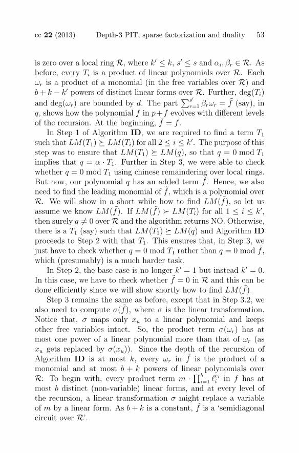
is zero over a local ring R, where k′ ≤ k, s′ ≤ s and αi, βr ∈ R. Asbefore, every Ti is a product of linear polynomials over R. Eachωr is a product of a monomial (in the free variables over R) andb + k − k′ powers of distinct linear forms over R. Further, deg(Ti)

and deg(ωr) are bounded by d. The part∑s′

r=1 βrωr = f (say), inq, shows how the polynomial f in p+f evolves with different levelsof the recursion. At the beginning, f = f .

In Step 1 of Algorithm ID, we are required to find a term T1

such that LM(T1) � LM(Ti) for all 2 ≤ i ≤ k′. The purpose of thisstep was to ensure that LM(T1) � LM(q), so that q = 0 mod T1

implies that q = α · T1. Further in Step 3, we were able to checkwhether q = 0 mod T1 using chinese remaindering over local rings.But now, our polynomial q has an added term f . Hence, we alsoneed to find the leading monomial of f , which is a polynomial overR. We will show in a short while how to find LM(f), so let usassume we know LM(f). If LM(f) � LM(Ti) for all 1 ≤ i ≤ k′,then surely q �= 0 over R and the algorithm returns NO. Otherwise,there is a T1 (say) such that LM(T1) � LM(q) and Algorithm IDproceeds to Step 2 with that T1. This ensures that, in Step 3, wejust have to check whether q = 0 mod T1 rather than q = 0 mod f ,which (presumably) is a much harder task.

In Step 2, the base case is no longer k′ = 1 but instead k′ = 0.In this case, we have to check whether f = 0 in R and this can bedone efficiently since we will show shortly how to find LM(f).

Step 3 remains the same as before, except that in Step 3.2, wealso need to compute σ(f), where σ is the linear transformation.Notice that, σ maps only xu to a linear polynomial and keepsother free variables intact. So, the product term σ(ωr) has atmost one power of a linear polynomial more than that of ωr (asxu gets replaced by σ(xu)). Since the depth of the recursion ofAlgorithm ID is at most k, every ωr in f is the product of amonomial and at most b + k powers of linear polynomials overR: To begin with, every product term m · ∏b

i=1 �eii in f has at

most b distinct (non-variable) linear forms, and at every level ofthe recursion, a linear transformation σ might replace a variableof m by a linear form. As b + k is a constant, f is a ‘semidiagonalcircuit over R’.

54 Saha et al. cc 22 (2013)

Finally, in Step 4, we need to confirm that [LM(T1)]q = 0.For this, we may have to find [LM(f)]f , if LM(f) happens tobe the same as LM(T1). This is taken care of by the way wefind LM(f) which also gives us its coefficient. We now show howto find LM(f). (Note: at any recursive stage, with base ring R,the ‘monomials’ are in the free variables and thus it is implicit thatthey take precedence over the other variables that moved inside R.)

Dual representation of f—Let �d′be a term occurring in the

product ωr, where

� = a1xv1 + · · · + an′xvn′ + τ

is a linear polynomial over R. (Assume that xv1 , . . . xvn′ are thefree variables over R). Replace τ by a formal variable z and useTheorem 2.1 to express (a1xv1 + · · · + an′xvn′ + z)d′

as

(a1xv1 + · · · + an′xvn′ + z)d′=

(n′+1)d′+1∑

i=1

gi(z) · gi1(xv1) . . . gin′(xvn′ ),

where gi and gij are univariates over F of degree at most d′. There-fore, �d′

can be expressed as

�d′=

(n′+1)d′+1∑

i=1

γi · gi1(xv1) . . . gin′(xvn′ ),

where γi = gi(τ) ∈ R, in time poly(n, d, dimF R). Since ωr is aproduct of a monomial (in xv1 , . . . , xvn′ ) and at most b+k productsof powers of linear forms over R, using the above equation, eachωr can be expressed as

ωr =

O((nd)b+k)∑

i=1

γi,r · gi1,r(xv1) . . . gin′,r(xvn′ ),

where γi,r ∈ R and gij,r is a polynomial over F of degree O((b+k)d),in time poly((nd)b+k, dimF R). Therefore, given the polynomial fits representation (reusing symbols γi and gij)


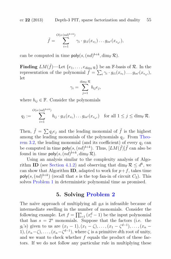
f =

O(s·(nd)b+k)∑

i=1

γi · gi1(xv1) . . . gin′(xvn′ ),

can be computed in time poly(s, (nd)b+k, dimF R).

Finding LM(f)—Let {e1, . . . , edimF R} be an F-basis of R. In therepresentation of the polynomial f =

∑i γi · gi1(xv1) . . . gin′(xvn′ ),

let

γi =

dimF R∑

j=1

bijej,

where bij ∈ F. Consider the polynomials

qj :=

O(s·(nd)b+k)∑

i=1

bij · gi1(xv1) . . . gin′(xvn′ ) for all 1 ≤ j ≤ dimF R.

Then, f =∑

qjej and the leading monomial of f is the highestamong the leading monomials of the polynomials qj. From Theo-rem 3.2, the leading monomial (and its coefficient) of every qj canbe computed in time poly(s, (nd)b+k). Thus, [LM(f)]f can also befound in time poly(s, (nd)b+k, dimF R).

Using an analysis similar to the complexity analysis of Algo-rithm ID (see Section 4.1.2) and observing that dimF R ≤ dk, wecan show that Algorithm ID, adapted to work for p+f , takes timepoly(s, (nd)b+k) (recall that s is the top fan-in of circuit C2). Thissolves Problem 1 in deterministic polynomial time as promised.

5. Solving Problem 2

The naıve approach of multiplying all gis is infeasible because ofintermediate swelling in the number of monomials. Consider thefollowing example. Let f =

∏ni=1 (xd

i − 1) be the input polynomialthat has s = 2n monomials. Suppose that the factors (i.e. thegi’s) given to us are (x1 − 1), (x1 − ζ), . . . , (x1 − ζd−1), . . . , (xn −1), (xn−ζ), . . . , (xn−ζd−1), where ζ is a primitive dth root of unity,and we want to check whether f equals the product of these fac-tors. If we do not follow any particular rule in multiplying these

56 Saha et al. cc 22 (2013)

factors, then we may as well end up with the intermediate prod-uct,

∏ni=1 (xd−1

i + xd−2i + · · · + 1), which has dn = slog d monomials.

Thus, given f with s monomials, we might have to spend time andspace O(slog d) if we follow this naıve approach.

Notice that, when gis are linear polynomials, Problem 2becomes a special case of Problem 1 and can therefore be solvedin deterministic polynomial time. However, the approach given inSection 4 does not seem to generalize directly to the case when,instead of linear functions, gis are sums of univariates. This caseis handled in this section.

5.1. Checking divisibility by (a power of) a sum of uni-variates. Given g1, . . . , gt, group together the polynomials gisthat are just F-multiples of each other. After this is done, we needto check whether f is equal to a product of the form a · gd1

1 . . . gdtt

(reusing symbol t), where a ∈ F and gi �= b·gj for any b ∈ F if i �= j.Suppose gi and gj are coprime for i �= j. (This assumption is jus-tified later in Section 5.2 by essentially proving them irreducible).Then, Problem 2 gets reduced to the problem of checking divisi-bility followed by a comparison of the leading monomials of f anda · gd1

1 . . . gdtt . The latter is easy as we have f and gis explicitly.

Checking divisibility, however, is more technical and we do thatin this section. We once again use the tool of dual representation,but on a slightly more general form of semidiagonal polynomials.

Theorem 5.1. Checking divisibility of a sparse polynomial f bygd, where g is a sum of univariates, can be done in deterministicpolynomial time.

Proof. Let g =∑n

i=1 ui(xi), where ui is a univariate in xi.Assume without loss of generality that u1 �= 0. Consider replacingthe partial sum

∑ni=2 ui(xi) in g by a new variable y so that we

get a bivariate h = (u1(x1) + y)d, which is a sparse polynomial aswell. Let degx1

u1 = e. Given any power of x1, say xk1, we can

employ long division with respect to the variable x1 to find theremainder when xk

1 is divided by h. This division is possible sinceh is monic in x1. It is not hard to see that the remainder, say rk,


thus obtained is a bivariate in x1 and y with degree in x1 less thaned and degree in y at most k.

To check whether gd divides f , do the following. For everymonomial of f , replace the power of x1 occurring in the monomial,say xk

1, by the corresponding remainder rk. After the replacementprocess is over, completely multiply out terms in the resulting poly-nomial, say f(x1, x2, . . . , xn, y), and express it as sum of monomialsin the variables x1, . . . , xn and y. Now notice that

f mod gd = f(x1, x2, . . . , xn,n∑

i=2

ui(xi)).

Since degree of x1 in f is less than ed,

gd | f if and only if f(x1, x2, . . . , xn,n∑

i=2

ui(xi)) = 0.

Polynomial f with y evaluated at∑n

i=2 ui(xi) is of the formof a sum of products, where each product term looks like m ·(∑n

i=2 ui(xi))j for some monomial m and integer j. This form

is similar to that of a semidiagonal circuit (Definition 1.1), exceptthat

∑ni=2 ui(xi) is a sum of univariates instead of a linear form.

To test whether f(x1, x2, . . . , xn,∑n

i=2 ui(xi)) = 0, use Theo-rem 2.1 to express it as a sum of product of univariates. Finally,invoke Theorem 3.2 to test whether the corresponding sum of prod-uct of univariates is identically zero.

The time complexity of this reduction to identity testingincludes computing each remainder rk, which takes poly(k, ed) time.Assuming there are s monomials in f , to express f as a sumof monomials in x1, x2, . . . , y it takes poly(s,D, ed) time, whereD is the total degree of f . Accounting for the substitution ofy by

∑ni=2 ui(xi), the total reduction time is poly(n, s,D, ed).

Finally, testing whether f(x1, x2, . . . , xn,∑n

i=2 ui(xi)) is identicallyzero takes polynomial time (by Theorem 2.1 and Theorem 3.2).

�

5.2. Irreducibility of a sum of univariates. In this section,the polynomial gs are assumed to be sums of univariates. We show

58 Saha et al. cc 22 (2013)

that if gi and gj depend on at least three variables, then they areessentially irreducible. Hence, they are either coprime or same (upto a constant multiple). Of course, it is trivial to check the lattercase and this makes our Chinese remaindering idea workable.

Theorem 5.2. (Irreducibility) Let g be a polynomial over a fieldF that is a sum of univariates. Suppose g depends non-trivially onat least three variables. Then, either g is irreducible, or g is a p-thpower of some polynomial where p = char(F).

Remark. Such a statement is false when g is a sum of just twounivariates. For example, the real polynomial g := x4

1 + x42 has

factors (x21+x2

2±x1x2

√2) (which is not even a sum of univariates!).

Denote ∂h∂xi

by ∂ih for any polynomial h. We shall say a poly-nomial h is monic in variable x if the monomial in h of highestx-degree is free of other variables. We need the following observa-tions (with g of Theorem 5.2).

Observation 5.3. Let g = u · v be a non-trivial factorization.Then both u and v are monic in every variable that g depends on.In particular, they depend on every variable that g depends on.

Proof. If u is not monic in, say, x1, then fix an ordering amongthe variables such that x1 is the highest. Then, the leading mono-mial of g = u · v is a mixed term which is not possible. �

Observation 5.4. If g is not a p-th power of any polynomial thenit is square-free.

Proof. Suppose not, then g = u2v for some polynomials u andv. If g is not a p-th power, there must exist a variable xi such that0 �= ∂ig = 2uv∂iu + u2∂iv. Since u divides the RHS, u must bea univariate as ∂ig is a univariate in xi. But this forces g to be aunivariate as u is also a factor of g. �

Proof of Theorem 5.2. Assume that g is not a p-th powerof any polynomial. Then, there exists a variable, say x1, such that


∂1g �= 0. Suppose g = u · v; this means ∂ig = (∂iu)v + (∂iv)u.Denote by hxi=α, the polynomial h evaluated at xi = α, whereα ∈ F (the algebraic closure of F).

Claim 5.5. There exists an α ∈ F such that u(x1=α), v(x1=α) �= 0and they share a non-trivial common factor.

Assume that the claim is true. There are two variables other thanx1, say x2 and x3, that appear in g. Then, ∂2g = (∂2u)v + (∂2v)uimplies that

(∂2g)(x1=α) = ∂2g = (∂2u)(x1=α) v(x1=α) + (∂2v)(x1=α) u(x1=α).

Similarly, ∂3g = (∂3u)(x1=α) v(x1=α) + (∂3v)(x1=α) u(x1=α).

If both ∂2g and ∂3g are nonzero, then the last two equations implythat gcd

(u(x1=α), v(x1=α)

)(which is not 1, by Claim 5.5) must di-

vide ∂2g and ∂3g. But this leads to a contradiction since the partialderivatives are univariates in x2 and x3, respectively.

Suppose ∂2g is zero. Since g is square-free, u and v do not shareany factor and hence all of ∂2g, ∂2u and ∂2v are zero, which impliesthat every occurrence of x2 in g, u and v has exponent that is amultiple of p = char(F). Hence,

g′ = u′ · v′

where g(x1, x2, . . . , xn) =: g′(x1, xp2, . . . , xn)

u(x1, x2, . . . , xn) =: u′(x1, xp2, . . . , xn)

v(x1, x2, . . . , xn) =: v′(x1, xp2, . . . , xn).

By inducting on this equation, we get the desired contradiction.�

Proof of Claim 5.5. Suppose g1 = ∂1g, u1 = ∂1u and v1 =∂1v, and let w = gcd(g1, u1, v1) which is a univariate in x1 as g1 isa univariate. Consider the following equation

0 �= g1

w=

(u1

w

)v +

(v1

w

)u.

Firstly, neither of u1 and v1 is zero. This is because, if u1 = 0 theng1 = v1 · u. This then forces u to be a univariate in x1, which is

60 Saha et al. cc 22 (2013)

not possible as u is also a factor of g. Since x1-degree of u1 is lessthan that of g1, the univariate g1/w has degree in x1 at least one.Let α ∈ F be a root of g1/w. Substituting x1 = α in the aboveexpression, we get an equation of the form

(5.6) u · vx1=α + v · ux1=α = 0,

where u = (u1/w)x1=α and v = (v1/w)x1=α. The above equation isnontrivial as none of u · vx1=α and v ·ux1=α is zero. This is becausenone of the polynomials ux1=α and vx1=α can be zero as they arefactors of gx1=α. Also, none of u and v is zero, as g1/w, u1/w andv1/w do not share any common factor, in particular x1 − α.

Now notice that, since u is monic in x2 (by Observation 5.3),degree of x2 in u1 is strictly less than that in u. Which means,degree of x2 in u is also strictly less than degree of x2 in ux1=α.Therefore, by treating the terms u, v, ux1=α, vx1=α as polynomialsin x2 over the function field F (x3, . . . , xn), we can conclude from(5.6) that ux1=α and vx1=α must share a nontrivial factor. �

5.3. Finishing the argument. In Section 5.1, we had promisedto later show that the polynomials g1, . . . , gt are irreducible.Although Theorem 5.2 justifies our assumption when gi dependson three or more variables, we need to slightly change our strategyfor bivariates and univariates. In this case, we first take pair-wise gcd of the bivariates (similarly, pairwise gcd of the univari-ates) and factorize accordingly till all the bivariates (similarly, theunivariates) are mutually coprime. Taking gcd of two bivariate(monic) polynomials takes only polynomial time using Euclideangcd algorithm (by long division). Once coprimeness is ensured, wecan directly check whether a bivariate gdi

i divides f by expressingf as f =

∑j fjmj, where fjs are bivariate polynomials depending

on the same two variables as gi, and mjs are monomials in theremaining variables. Then,

gdii | f if and only if gdi

i | fj for all j.

Once again, just like gcd, bivariate divisibility is a polynomial timecomputation (simply by long division). Finally, we can use Chineseremaindering to complete the argument in a similar fashion as inSection 5.1.


To summarize, we can check whether f =∏t

i=1 gi, where gis aresums of univariates, in time poly(n, t, d, s), where d is the boundon the total degrees of f and the gi’s, and s is the number ofmonomials (with nonzero coefficients) in f . It is the property ofthe coprimality of different gis that helped us reduce the problemto checking divisibility, which was then handled using the dualrepresentation.

6. Extensions to small characteristic fields

Over fields of small characteristics, the dual representation forsemidiagonal circuit has to be modified slightly. The followingsection gives an appropriate modification.

6.1. Preliminaries: The dual representation. This is a ver-sion of Theorem 2.1 that applies for fields of small characteristicsby moving to appropriate Galois rings (like Galois fields but withprime-power characteristic!).

Theorem 6.1. Given f = (∑n

i=1 gi(xi))D, where gi is a univariate

in xi of degree at most d over a field F of characteristic p, we canfind an integer N ≤ poly(n,D) such that pNf can be expressedas a sum of (nD +1) products of univariates of degree dD over thering Z/pN+1

Z, in poly(n, d,D) time.

Proof. Our main trick is to do computations on f over a ringof p-power characteristic. To exhibit this trick let us assume that F

is a prime field Fp. Consider∑n

i=1 gi(xi) as a polynomial over therationals (i.e. view Fp as integers {0, . . . , p−1}), then Theorem 2.1gives an expression for f :

f =nD+1∑

i=1

n∏

j=1

gij(xj).

Some of the coefficients on the RHS might be rationals with pow-ers of p appearing in the denominator. By multiplying the aboveexpression by a suitably large power of p (e.g., the largest power

62 Saha et al. cc 22 (2013)

in any denominator), the above can be rewritten as:

pN · f =∑

i

∏

j

g′ij(xj),

where the coefficients on the RHS are free of any p’s in the denom-inator. Therefore, this is a nontrivial expression for pN · f in thering Z/pN+1

Z, as claimed. �

In the case of finite base field Fq = Fp[x]/(μ(x)) with the leadingcoefficient of μ being one, we begin by considering f as a polyno-mial over the field Q[x]/(μ(x)) (note: μ(x) remains irreducible overQ). Now the above proof proceeds in exactly the same way, therebyobtaining a nontrivial expression for pN · f over the (Galois) ringZ[x]/(pN+1, μ(x)).

In the case of characteristic p but infinite base field Fp(t), webegin by considering f as a polynomial over the field Q(t). Theabove proof gives a nontrivial expression for pN · f over the ring:(Z/pN+1

Z)[t] localized by its set of nonzerodivisors.

Thus, using a combination of the above tricks, we can get adual representation over any extension of Fp.

With this modified dual representation, Problem 1 and Prob-lem 2 can be tackled the same way as outlined earlier. The onlyadditional requirement is to find the leading monomial and theassociated coefficient of a semidiagonal circuit over these rings ofprime-power characteristic.

6.2. Finding the leading monomial of semidiagonal cir-cuits. Given a semidiagonal circuit f , Theorem 6.1 can be used(repeatedly) to write pNf as a sum of product of univariates overa ring Z/pN+1

Z. If f =∑

αmm, where m is a monomial and αm

is the associated coefficient, then pNf =∑

(pNαm)m. Therefore,if we can find the leading monomial and coefficient of pNf overZ/pN+1

Z, we can derive the leading monomial and coefficient off . Thus, we need a version of Theorem 3.2 over rings of the formZ/pN+1

Z.One of the key elements in the proof of Theorem 3.2 is that we

can prune down the list of vectors {c1, . . . , cr} from Fk to always

ensure that we have the vector contributing to the leading mono-


mial in our set. For this, we required a “dimension argument” thatstates that if r > k, then there exists an i such that ci can be writ-ten as a linear combination of the lower indexed vectors. This istrivial in the case of vector spaces.

While working over more general rings, we need to work with‘vectors’ (abusing terminology) over rings of the form Z/pN

Z. Un-like the case when we are working over a field, a linear combinationof the form

∑αici = 0 does not necessarily translate to writing

one of the ci’s as a combination of the preceding vectors since someof the coefficients in the linear combination might not be invert-ible. For example, if v is the column vector (pN−1, pN−2, . . . , 1)T

and 0 = (0, . . . , 0)T is the column vector of N zeroes, then noneof the Nk rows of the following matrix can be written as a linearcombination of the preceding rows:

⎡

⎢⎢⎢⎣

v 0 · · · 00 v · · · 0...

.... . .

...0 0 · · · v

⎤

⎥⎥⎥⎦

Nk×k

.

However, the following lemma shows that such a linear combi-nation would indeed exist if we had more than Nk vectors.

Lemma 6.2. Let {c1, . . . , c1} be elements of(Z/pN

Z)k

. If r >Nk, then there exists an i such that c1 can be written as a linearcombination of {c1, . . . , ci−1}. That is,

ci =i−1∑

j=1

αjcj where αj’s are from Z/pNZ.

Proof. Given an ordered set of vectors {c1, . . . , cr}, we shallcall a linear combination

∑αjcj a “monic” linear combination if

the highest indexed ci appearing in the linear combination hascoefficient 1.

Construct the r × k matrix whose rows are from {c1, . . . , cr}.The goal is to repeatedly apply “monic row transformations” thatis replacing a row ci by ci − ∑

j<i αjcj. This would eventually

64 Saha et al. cc 22 (2013)

induce a zero row, which will give us our desired linear combination.The proof proceeds by induction, handling one coordinate at atime.

Let i be the smallest index (if it exists) such that the firstcoordinate of ci is nonzero modulo p. Replace every other (higherindexed) row cj by (cj − αjci) to ensure that its first coordinate isnow zero modulo p. Observe that these transformations are monic.The first coordinate of every row, besides ci, will now be divisibleby p. Dropping row i, we repeat the procedure to make all of themzero modulo p2, and similarly for p3 etc. Thus, by dropping atmost N rows, we can ensure that the first coordinate of every rowis 0 (modulo pN).

We are now left with {d1, . . . ,dr′}, with r′ > r − N , over(Z/pN

Z)k−1

and by induction we would find a monic linear com-bination of the dis that is zero. It is not hard to see that thistranslates to a monic linear dependence among the cis since weonly applied monic transformations. �

With this, we have a version of Theorem 3.2 over rings of prime-power characteristic.

Theorem 6.3. Given f =∑k

i=1

∏nj=1 gij(xj) over a ring Z/pN

Z,where gij is a univariate in xj of degree at most d, the leadingmonomial of f (and its coefficient) can be found in poly(nkdN)time.

It is now straightforward to show that Corollary 3.3 holds evenover small characteristic fields: just apply Theorem 6.1 repeatedlyand finally invoke Theorem 6.3.

6.3. Solving Problem 1. The proof proceeds along exactly thesame lines as described in Section 4.2. The only difference is whenwe have to compute the leading monomial and its coefficient of asemidiagonal circuit f =

∑βrωr over the local ring.

◦ In each linear polynomial appearing in ωr, replace the con-stant term τ by a fresh variable z. After repeated applicationsof Theorem 6.1 to such expressions and finally taking a sum,we get pN f =

∑γi · gi1(x1) · · · gin(xn) where x1, . . . , xn are


the free variables, and γi ∈ R (note: R is now of character-istic pN+1).

◦ Let {e1, . . . , edim R} be a (Z/pN+1Z)-basis of R, and let γi =∑

bijej. Then, the leading monomial and coefficient of pN fcan be computed from those of the polynomials qj =

∑i bij ·

gi1(x1) · · · , gin(xn).

◦ Compute the leading monomial and coefficient of each qj

using Theorem 6.3 and recover the leading monomial andcoefficient of f .

The other parts of the proof are independent of the character-istic of the field and hence go through in exactly the same way.

6.4. Solving Problem 2. Again all our arguments were inde-pendent of the field except when we invoke semidiagonal PIT inTheorem 5.1. At that point, we would now invoke Theorem 6.1and Theorem 6.3.

7. Discussion and open problems

We conclude by posing two open questions related to the problemsstudied here. The first relates to depth-4 fan-in 2 PIT.

Open Problem 1. Find a deterministic polynomial time algo-rithm to check whether f =

∏ti=1 gdi

i , where f is a sparsepolynomial and the gis are mutually coprime, bounded degree poly-nomials.

One particular case of interest is when the gis are quadraticforms. Observe that a polynomial gd divides f if and only if gdivides f and gd−1 divides ∂f

∂x1(assuming f depends on x1 and

deg(f) > char(F)). Since ∂f∂x1

is also sparse, using this observa-tion, the problem eventually boils down to checking whether gdivides h, where both g and h are sparse polynomials. Now sup-pose g is a quadratic form. It is known that there exists an effi-ciently computable linear transformation σ on the variables suchthat σ(g) =

∑ri=1 x2

i , which is a sum of univariates. The polyno-mial g divides h if and only if σ(g) divides σ(h). We have shown

66 Saha et al. cc 22 (2013)

how to divide a sparse polynomial by a sum of univariates. But,the issue here is that σ(h) need not be sparse—it is an image ofa sparse h under an invertible σ. Is it possible to resolve this issue?

The second relates to depth-4 higher fan-in PIT.

Open Problem 2. Find a deterministic polynomial time algo-rithm to solve PIT on depth-4 circuits with bounded top fan-in k,where each of the k multiplication gates is a product of sums ofunivariate polynomials.

Note that, a solution for k = 2 easily follows from Theorem 5.2and unique factorization. But, it is unclear how to solve this prob-lem even for k = 3. The problem can also be seen as a certaingeneralization of bounded top fan-in depth-3 PIT (Kayal & Sax-ena 2007) to the case of depth-4 circuits.

Acknowledgements

The second author is supported by the Microsoft Research (India)Ph.D Fellowship.

References

Manindra Agrawal (2005). Proving Lower Bounds Via Pseudo-random Generators. In Foundations of Software Technology and Theo-retical Computer Science, 92–105.

Manindra Agrawal & Somenath Biswas (1999). Primality andIdentity Testing via Chinese Remaindering. Proceedings of the 40thAnnual IEEE Symposium on Foundations of Computer Science, NewYork City NY 202–209.

Manindra Agrawal, Neeraj Kayal & Nitin Saxena (2004).PRIMES is in P. Annals of Mathematics 160(2), 781–793.

Manindra Agrawal & Ramprasad Saptharishi (2009). Classify-ing polynomials and identity testing. Current Trends in Science, IndianAcademy of Sciences 149–162.


Manindra Agrawal & V Vinay (2008). Arithmetic circuits: A chasmat depth four. Proceedings of the 49th Annual IEEE Symposium onFoundations of Computer Science, Philadelphia PA 67–75.

Sanjeev Arora, Carsten Lund, Rajeev Motwani, Madhu

Sudan & Mario Szegedy (1998). Proof Verification and the Hardnessof Approximation Problems. Journal of the ACM 45(3), 501–555.

Zhi-Zhong Chen & Ming-Yang Kao (1997). Reducing Randomnessvia Irrational Numbers. Proceedings of the Twenty-ninth Annual ACMSymposium on Theory of Computing, El Paso TX 200–209.

Michael Clausen, Andreas W. M. Dress, Johannes Grabmeier

& Marek Karpinski (1991). On Zero-Testing and Interpolation ofk-Sparse Multivariate Polynomials Over Finite Fields. Theoretical Com-puter Science 84(2), 151–164.

Joachim von zur Gathen (1983). Factoring Sparse MultivariatePolynomials. Proceedings of the 24th Annual IEEE Symposium onFoundations of Computer Science, Tucson AZ 172–179.

Valentine Kabanets & Russell Impagliazzo (2003). Derandom-izing polynomial identity tests means proving circuit lower bounds.Proceedings of the Thirty-fifth Annual ACM Symposium on Theory ofComputing, San Diego CA 355–364.

Neeraj Kayal & Nitin Saxena (2007). Polynomial Identity Testingfor Depth 3 Circuits. Computational Complexity 16(2), 115–138.

Adam Klivans & Daniel A. Spielman (2001). Randomness efficientidentity testing of multivariate polynomials. Proceedings of the Thirty-third Annual ACM Symposium on Theory of Computing, Hersonissos,Crete, Greece 216–223.

Pascal Koiran & Sylvain Perifel (2007). The complexity oftwo problems on arithmetic circuits. Theoretical Computer Science389(1-2), 172–181.

Daniel Lewin & Salil P. Vadhan (1998). Checking PolynomialIdentities over any Field: Towards a Derandomization? Proceedingsof the Thirtieth Annual ACM Symposium on Theory of Computing,Dallas TX 438–447.

68 Saha et al. cc 22 (2013)

Laszlo Lovasz (1979). On determinants, matchings, and randomalgorithms. In Fundamentals of Computation Theory, 565–574.

Carsten Lund, Lance Fortnow, Howard J. Karloff & Noam

Nisan (1990). Algebraic Methods for Interactive Proof Systems. Pro-ceedings of the 31st Annual IEEE Symposium on Foundations of Com-puter Science, St. Louis MO 2–10.

Ran Raz (2010). Tensor-rank and lower bounds for arithmetic formu-las. In Proceedings of the Fourty-second Annual ACM Symposium onTheory of Computing, Cambridge, MA, USA, 659–666.

Ran Raz & Amir Shpilka (2004). Deterministic Polynomial IdentityTesting in Non-Commutative Models. Proceedings of the 19th IEEEConference on Computational Complexity, Amherst MA 215–222.

Shubhangi Saraf & Ilya Volkovich (2011). Black-box identitytesting of depth-4 multilinear circuits. Proceedings of the Fourty-thirdAnnual ACM Symposium on Theory of Computing, San Jose CA.

Nitin Saxena (2008). Diagonal Circuit Identity Testing and LowerBounds. In Proceedings of the 35th International Colloquium onAutomata, Languages and Programming ICALP, Reykjavik Iceland,60–71.

Nitin Saxena (2009). Progress on Polynomial Identity Testing. Bul-letin of the European Association for Theoretical Computer Science(90), 49–79.

Nitin Saxena & C. Seshadhri (2011). Blackbox identity testing forbounded top fanin depth-3 circuits: the field doesn’t matter. Proceed-ings of the Fourty-third Annual ACM Symposium on Theory of Com-puting, San Jose CA.

Jacob T. Schwartz (1980). Fast Probabilistic Algorithms for Verifi-cation of Polynomial Identities. Journal of the ACM 27(4), 701–717.

Adi Shamir (1990). IP=PSPACE. In Proceedings of the 31st AnnualIEEE Symposium on Foundations of Computer Science, St. Louis MO,11–15.

Amir Shpilka & Amir Yehudayoff (2010). Arithmetic Circuits: Asurvey of recent results and open questions. Proceedings of the 51st


Annual IEEE Symposium on Foundations of Computer Science 5(3-4),207–388.

Richard Zippel (1979). Probabilistic algorithms for sparse polynomi-als. EUROSAM 216–226.

Manuscript received 18 April 2011

Chandan Saha

Max Plank Institute forInformatics,

66123 Saarbrucken, [email protected]://www.mpi-inf.mpg.de/∼csaha/

Ramprasad Saptharishi

Chennai Mathematical Institute,Chennai 603103, [email protected]://www.cmi.ac.in/∼ramprasad/

Nitin Saxena

Hausdorff Center forMathematics,

Universitat Bonn,53119 Bonn, [email protected]://www.math.uni-bonn.de/∼saxena/

a case of depth-3 identity testing, sparse factorization and duality

Documents