entropy

Article

A Chain, a Bath, a Sink, and a Wall

Stefano Iubini 1,2,*, Stefano Lepri 2,3 ID , Roberto Livi 1,2,3, Gian-Luca Oppo 4 and Antonio Politi 5 ID

1 Dipartimento di Fisica e Astronomia, Università di Firenze, via G. Sansone 1, I-50019 Sesto Fiorentino, Italy;livi@fi.infn.it

2 Istituto Nazionale di Fisica Nucleare, Sezione di Firenze, via G. Sansone 1, I-50019 Sesto Fiorentino, Italy;stefano.lepri@isc.cnr.it

3 Consiglio Nazionale delle Ricerche, Istituto dei Sistemi Complessi, via Madonna del Piano 10,I-50019 Sesto Fiorentino, Italy

4 SUPA and Department of Physics, University of Strathclyde, Glasgow G4 0NG, UK; g.l.oppo@strath.ac.uk5 Institute for Complex Systems and Mathematical Biology & SUPA, University of Aberdeen,

Aberdeen AB24 3UE, UK; a.politi@abdn.ac.uk* Correspondence: stefano.iubini@unifi.it

Received: 22 June 2017; Accepted: 24 August 2017; Published: 25 August 2017

Abstract: We numerically investigate out-of-equilibrium stationary processes emerging in a DiscreteNonlinear Schrödinger chain in contact with a heat reservoir (a bath) at temperature TL anda pure dissipator (a sink) acting on opposite edges. Long-time molecular-dynamics simulationsare performed by evolving the equations of motion within a symplectic integration scheme. Mass andenergy are steadily transported through the chain from the heat bath to the sink. We observe twodifferent regimes. For small heat-bath temperatures TL and chemical-potentials, temperature profilesacross the chain display a non-monotonous shape, remain remarkably smooth and even enter theregion of negative absolute temperatures. For larger temperatures TL, the transport of energy isstrongly inhibited by the spontaneous emergence of discrete breathers, which act as a thermal wall.A strongly intermittent energy flux is also observed, due to the irregular birth and death of breathers.The corresponding statistics exhibit the typical signature of rare events of processes with largedeviations. In particular, the breather lifetime is found to be ruled by a stretched-exponential law.

Keywords: discrete nonlinear schrödinger; discrete breathers; negative temperatures; open systems

PACS: 05.60.-k; 05.70.Ln; 63.20.Pw

1. Introduction

The study of nonequilibrium thermodynamics of systems composed of a relatively smallnumber of particles is motivated by the need for a deeper theoretical understanding of the statisticallaws leading to the possibility of manipulating small-scale systems like biomolecules, colloids,or nano-devices. In this framework, statistical fluctuations and size effects play a major role andcannot be ignored as it is customary to do in their macroscopic counterparts.

Arrays of coupled classical oscillators are representative models of such systems and havebeen studied intensively in this context [1–3]. In particular, the Discrete Nonlinear Schrödinger(DNLS) equation has been widely investigated in various domains of physics as a prototype modelfor the propagation of nonlinear excitations [4–6]. In fact, it provides an effective description ofelectronic transport in biomolecules [7] as well as of nonlinear waves propagation in layered photonicor phononic systems [8,9]. More recently, a renewed interest for this multi-purpose equation emergedin the physics of gases of ultra-cold atoms trapped in optical lattices (e.g., see [10] and referencestherein for a recent survey).

Entropy 2017, 19, 445; doi:10.3390/e19090445 www.mdpi.com/journal/entropy

Entropy 2017, 19, 445 2 of 15

The DNLS dynamics are characterized by two conserved quantities: the energy density h and themass density a (also termed norm—see the following section for their definitions). Therefore, a genericthermodynamic state of the DNLS equation can be seen as a point in the (a, h) plane. The equilibriumthermodynamics of the DNLS model was studied in a seminal paper by Rasmussen et al. [11] withinthe grand-canonical formalism. Here, it was shown that an equation of state can be formally derivedwith the help of transfer–integral techniques. Accordingly, any thermodynamic equilibrium state (a, h)can be equivalently represented in terms of a temperature T and a chemical potential µ which can benumerically determined by implementing suitable microcanonical definitions [12,13]. In Reference [11],it was found that a line of infinite–temperature equilibrium states in the (a, h) plane separates standardthermodynamic states, characterized by a positive T, from those characterized by negative absolutetemperatures. The existence of negative temperatures can be traced back to the properties of the twoconserved quantities of the system. From the point of view of dynamics, it was realized that negativetemperatures can be associated to the presence of intrinsically localized excitations, named discretebreathers (DB) (see e.g., [14–16]). In a series of important papers, Rumpf developed entropy-basedarguments to describe the asymptotic states above this infinite-temperature line [17–20]. It has beenlater found that negative–temperature states can form spontaneously via the dynamics of the DNLSequation. They persist over extremely long time scales, that might grow exponentially with systemsize as a result of an effective mechanism of ergodicity–breaking [21].

A related question is whether the dynamics of the system influences non-equilibrium propertieswhen the system exchanges energy and/or mass with the environment. In a series of papers [21–23],it has been found that when pure dissipators act at both edges of a DNLS chain (a case sometimescalled boundary cooling [24–27]) the typical final state consists of an isolated static breather embeddedin an almost empty background. The breather collects a sensible fraction of the initial energy and it isessentially decoupled from the rest of the chain. The spontaneous creation of localized energy spotsout of fluctuations has further consequences on the relaxation to equipartition, since the interactionwith the remaining part of the chain can become exponentially weak [28,29]. A similar phenomenonoccurs after a quench from high to low temperatures in oscillator lattices [30]. Also, boundary drivingby external forces may induce non-linear localization [31–33].

When, instead, the chain is put in contact with thermal baths at its edges, non-equilibriumstationary states characterized by a gradient of temperature and chemical potential emerge [13].Local equilibrium is typically satisfied so that the overall state of the chain can be convenientlyrepresented as a path in the (a, h) plane connecting two points corresponding to the thermodynamicvariables imposed by the two reservoirs. The associated transport of mass and energy is typicallynormal (diffusive) and can be described in terms of the Onsager formalism. However, peculiar features,such as non-monotonous temperature profiles [34] or persistent currents [35], are found as well asa signature of anomalous transport in the low-temperature regime [36,37].

In this paper we consider a set-up where one edge is in contact with a heat reservoir at temperatureTL and chemical potential µL, while the other interacts with a pure dissipator, i.e., a mass sink.The original motivation for studying this configuration was to better understand the role of DBs inthermodynamic conditions. At variance with standard set-ups [1,2], this is conceptually closer toa semi-infinite array in contact with a single reservoir. In fact, on the pure-dissipator side, mass canonly flow out of the system.

The presence of a pure dissipator forces the corresponding path to terminate close to the point(a = 0, h = 0), which is singular both in T and µ. This is indeed the point where the infinite- and thezero-temperature lines collapse. Therefore, slight deviations may easily lead to crossing the β = 0line, where β = 1/T is the inverse temperature. This is indeed the typical scenario observed for smallTL, when β smoothly changes sign twice before approaching the dissipator (see Figure 1 for a fewsampled paths). The size of the negative-temperature region increases with TL and appears to be stableover long time scales. Upon further increasing TL, a different stationary regime is found, characterizedby strong fluctuations of mass and energy flux. In practice, the negative-temperature region first

Entropy 2017, 19, 445 3 of 15

extends up to the dissipator edge and then it progressively shrinks in favour of a positive-temperatureregion (on the other side of the chain). In this regime, the dynamics are controlled by the spontaneousformation (birth) and disappearance (death) of discrete breathers.

0 0.5 1

a

-1

0

1

2

h

Figure 1. Phase diagram of the DNLS equation in the (a− h) plane of, respectively, energy and massdensities. The positive-temperature region extends between the ground state β = +∞ line (solid bluelower curve) and the β = 0 isothermal (red dashed curve). Purple circles show the µ = 0 line, whichhas been determined numerically through equilibrium simulations (data are taken from Reference [13]).Black curves refer to nonequilibrium profiles obtained by employing a heat bath with parametersTL = 3 and µL = 0 and a pure dissipator located at the left and right edges of the chain, respectively.Dotted, dot-dashed, dot-dot-dashed and solid curves refer to chain sizes N = 511, 1023, 2047, and4095, respectively. Upon increasing N, these above profiles tend to enter the negative temperatureregion. Simulations are performed by evolving the DNLS chain over 107 time units after a transientof 4× 107 units. For the system size N = 4095, a further average over 10 independent trajectoriesis performed.

In Section 2 we introduce the model and briefly recall the definition of the main observables.Section 3 is devoted to a detailed characterization of the low-temperature phase, while thefar-from-equilibrium phase observed for large TL is discussed in Section 4. This is followed bythe analysis of the statistical properties of the birth/death process of large-amplitude DBs, illustratedin Section 5. Finally, in Section 6 we summarize the main results and comment about possiblerelationships with similar phenomena previously reported in the literature.

2. Model and Methods

We consider a DNLS chain of size N and with open boundary conditions, whose bulk dynamicsis ruled by the equation

izn = −2|zn|2zn − zn−1 − zn+1 (1)

where (n = 1, . . . , N) and zn = (pn + iqn)/√

2 are complex variables, with qn and pn being standardconjugate canonical variables. The quantity an = |zn(t)|2 can be interpreted as the number of particles,or, equivalently, the mass in the lattice site n at time t. Upon identifying the set of canonical variableszn and iz∗n, Equation (1) can be read as the equation of motion generated by the Hamiltonian functional

H =N

∑n=1

(|zn|4 + z∗nzn+1 + znz∗n+1

)(2)

Entropy 2017, 19, 445 4 of 15

through the Hamilton equations zn = −∂H/∂(iz∗n). We are dealing with a dimensionless version ofthe DNLS equation: the nonlinear coupling constant and the hopping parameters, which are usuallyindicated explicitly in the Hamiltonian (2), have been set equal to unity. Accordingly, also the timevariable t is expressed in arbitrary adimensional units. Without loss of generality, this formulation hasthe advantage of simplifying numerical simulations.

A relevant property of the DNLS dynamics is the existence of a second conserved quantity besidethe total energy H, namely the total mass

A =N

∑n=1|zn|2 . (3)

As a result, an equilibrium state is specified by two parameters, the mass density a = A/N ≥ 0and the energy density h = H/N. The first reconstruction of the equilibrium phase-diagram (a, h) ofthe DNLS equation was reported in [11]. It is reproduced in Figure 1 for our choice of parameters,where the lower solid line defines the (T = 0) ground-state line h = a2 − 2a for different values of themass density a. The ground-state corresponds to a uniform state with constant amplitude and constantphase-differences zn =

√aei(µt+πn), with µ = 2(a − 1). States below this curve are not physically

accessible. The positive-temperature region lies above the ground-state up to the red dashed lineh = 2a2, which corresponds to the infinite-temperature (β = 0) line. In this limit, the grand-canonicalequilibrium distribution becomes proportional to exp (βµA), where the finite (negative) productβµ implies a diverging chemical potential. Equilibrium states at infinite temperature are thereforecharacterized by an exponential distribution of the amplitudes P(|zn|2) = a−1e−|zn |2/a and randomphases. Finally, states above the β = 0 line belong to the so-called negative-temperature region [11,21].

Finite-temperature equilibrium states do not allow for straightforward analytical treatments.However, one can determine the relation a(T, µ), h(T, µ) numerically, by putting the systemin interaction with an external reservoir (see below) that imposes T and µ and by measuringthe corresponding equilibrium densities. This method was adopted in Reference [13] to identify the µ = 0line shown in Figure 1. Upon increasing µ, the curve moves to the right in the (a, h) diagram and becomesmore and more vertical (data not shown). Isothermal lines T = c can be found analogously: they roughlyfollow the profile of the T = 0 line and, upon increasing c, they span all the positive-temperatureregion, approaching the infinite-temperature line for c→ +∞ [13].

A non-equilibrium steady state can be represented as a path in the (a, h)-parameter space,where a(x) is the mass density, h(x) the energy density, and x = n/N the rescaled position alongthe chain. In our set-up, the first site of the chain (n = 1) is in contact with a reservoir at temperatureTL and chemical potential µL. This is ensured by implementing the non-conservative Monte-Carlodynamics described in Reference [13]. In a few words, the reservoir performs random perturbationsδz1 = (δp1 + iδq1)/

√2 of the state variable z1 that are accepted or rejected according to

a grand-canonical Metropolis cost-function exp [−TL(∆H− µL∆A)], where ∆H and ∆A are respectivelythe variations of energy and mass produced by δz1. The perturbations δp1 and δq1 areindependent random variables extracted from a uniform distribution in the interval [−R, R].The opposite site (n = N) interacts with a pure stochastic dissipator that sets the variable zN equal to zero,thus absorbing an amount of mass equal to |zN|2. Both the heat bath and the dissipator are activatedat random times, whose separations are independent and identically distributed variables uniformlydistributed within the interval [tmin, tmax]. On average, this corresponds to simulating an interactionprocess with decay rate γ ∼ t−1, where t = (tmax + tmin)/2. Notice that different prescriptions,such as for example a Poissonian distribution of times with average t or a constant pace equal to t,do not introduce any relevant modification in the dynamical and statistical properties of the model (1).Finally, the Hamiltonian dynamics between successive interactions with the environment has beengenerated by implementing a symplectic, 4th-order Yoshida algorithm [38]. We have verified that atime step ∆t = 2× 10−2 suffices to ensure suitable accuracy.

Entropy 2017, 19, 445 5 of 15

Throughout the paper we deal with measurements of temperature profiles. Since the DNLSHamiltonian is not separable, the standard relation between temperature and local kinetic energydoes not hold. Due to the existence of the second conserved quantity A, it is necessary to make use ofthe microcanonical definition provided in [39] and further extended in [12]. Its derivation is foundedon the thermodynamic relation

β = T−1 =∂S∂E

∣∣∣∣A=M

(4)

for a system with total energy H = E, total mass A = M and entropy S. The calculation amounts toderive a measure of the hyper-surface at constant energy and mass in the phase space and to computeits variation with respect to E at constant mass. The general expression of T is a thermal average ofa non-local function of the dynamical variables zn and z∗n and is rather involved; we refer to [13,21]and the related bibliography for theoretical and computational details.

In what follows, we consider a situation where all parameters, other than TL, are kept fixed.In particular, we have chosen µL = 0, R = 0.8 and t = 3× 10−2, with tmax and tmin of order 10−2. We haveverified that the results obtained for this choice of the parameter values are general. A more detailedaccount of the dependence of the results on the thermostat properties will be reported elsewhere.

Finally, we recall the observables that are typically used to characterize a steady-state out ofequilibrium: the mass flux

ja = 2〈Im(z∗nzn+1)〉 , (5)

and the energy fluxjh = 2〈Re(znz∗n+1)〉 , (6)

where the angular brackets denote a time average.

3. Low-Temperature Regime: Coupled Transport and Negative Temperatures

In the left panel of Figure 2, we report the average profile of the inverse temperature β(x)as a function of the rescaled site position x = n/N, for different values of the temperature ofthe thermostat. A first “anomaly” is already noticeable for relatively small TL: the profile isnon monotonous (see for example the curve for TL = 1). This feature is frequently encounteredwhen a second quantity, besides energy, is transported [13,40,41]. In the present setup, this secondthermodynamic observable is the chemical potential µ(x), set equal to zero at the left edge. Rather thanplotting µ(x), in the right panel of Figure 2, we have preferred to plot the more intuitive mass densitya(x). There we see that the profile for TL = 1 deviates substantially from a straight line, indicating thatthe thermodynamic properties vary significantly along the chain and suggesting that the lattice mightnot be long enough to ensure an asymptotic behavior.

To clarify this point, we have performed simulations for different values of N. The resultsfor TL = 1 are reported in Figure 3, where we plot the local temperature T as a function of x.All profiles start from T = 1, the value imposed by the thermostat and, after an intermediate bump,eventually attain very small values. Since neither the temperature nor the chemical potential aredirectly imposed by the purely dissipating “thermostat”, it is not obvious to predict the asymptoticvalue of the temperature (and the chemical potential). The data reported in the inset suggest a sortof logarithmic growth with N, but this is not entirely consistent with the results obtained for TL = 3(see below).

If transport were normal and N were large enough, the various profiles should collapse ontoeach other, but this is far from the case displayed in Figure 3. The main reason for the lack ofconvergence is the growth of the temperature bump. This is because, upon further increases of N,the system spontaneously crosses the infinite temperature line and enters the negative-temperatureregion. For TL = 3, this “transition” has already occurred for N = 4095, as it can be seen in Figure 2.The crossings of the infinite temperature points (β = 0) at the boundaries of the negative temperatureregion correspond to infinite (negative) values of the chemical potential µ in such a way that the

Entropy 2017, 19, 445 6 of 15

product βµ remains finite at these turning points (data not reported). To our knowledge, this is thefirst example of negative-temperature states robustly obtained and maintained in nonequilibriumconditions in a chain coupled with a single reservoir at positive temperature. In order to shed light onthe thermodynamic limit, we have performed further simulations for different system sizes. In Figure 4,we report the results obtained for TL = 3 and N ranging from 511 to 4095. In Figure 4a, we see that thenegative-temperature region is already entered for N = 1023. Furthermore, its extension grows withN, suggesting that in the thermodynamic limit it would cover the entire profile but the edges.

Since non-extensive stationary profiles have been previously observed both in a DNLS and a rotorchain (i.e., the XY-model in d = 1) at zero temperature and in the presence of chemical potentialgradients [42], it is tempting to test to what extent an anomalous scaling (say n/

√N) can account

for the observations. In the inset of Figure 4a, we have rescaled the position along the lattice by√

N.For relatively small but increasing values of n/

√N we do see a convergence towards an asymptotic

curve, which smoothly crosses the β = 0 line. This suggests that close to the left edge, positivetemperatures extend over a range of order O(

√N), thereby covering a non-extensive fraction of

the chain length. The scaling behavior in the rest of the chain is less clear, but it is possibly a standardextensive dynamics characterized by a finite temperature on the right edge. A confirmation ofthe anomalous scaling in the left part of the chain is obtained by plotting the profiles of h and a againas a function of n/

√N (see the panels (b) and(c) in Figure 4, respectively). Further information can be

extracted from the scaling behavior of the stationary mass flux ja. In Figure 5, we report the averagevalue of ja as a function of the lattice length. There, we see that ja decreases roughly as N−1/2. At afirst glance this might be interpreted as a signature of energy super-diffusion, but it is more likely dueto the presence of a pure dissipation on the right edge (in analogy to what seen in the XY-model [43]).

Figure 2. Average profiles of the inverse temperature β(x) (panel (a)) and mass-density a(x) (panel (b))for a DNLS chain with N = 4095 and different temperatures TL of the reservoir acting at the leftedge, where µ = 0. The profile β(x) is computed making use of the microcanonical definition oftemperature. Simulations are performed evolving the DNLS chain over 107 time units after a transientof 4× 107 units. In order to obtain a reasonable smoothing of these time-averaged profiles we havefurther averaged each of them over 10 independent trajectories.

Entropy 2017, 19, 445 7 of 15

0 0.2 0.4 0.6 0.8 1x = n/N

0

1

2

3

T(x)

N = 511N = 1023N = 2047N = 4095

102

103 N

-4

0

4β

R,µ

R

Figure 3. Average profiles of the temperature T(x) for TL = 1 and different system sizes N. The profileT(x) is computed by means of the microcanonical definition of temperature. The inset shows theboundary inverse temperature βR (black circles) and chemical potential µR (red squares) close to thedissipator side as a function of the system size N. The data refers to the microcanonical definitionsof temperature and chemical potential computed on the last 10 sites of the chain. Simulations areperformed evolving the system over 107 time units after a transient of 4× 107 units. For the systemsize N = 4095 a further average over 10 independent trajectories has been performed.

0 0.2 0.4 0.6 0.8 1

n/N

-0.5

0

0.5

1

1.5

2β

N = 511N = 1023N = 2047N = 4095

0 20 40 60

n/N1/2

0

1

2β

(a)

0

0.5

1

1.5h

0 10 20 30n/N

1/2

0

0.5

1a

(b)

(c)

Figure 4. Panel (a): average profiles of inverse temperature β for TL = 3 and different system sizesN. The profile β is computed by means of the microcanonical definition of temperature. In the inset,an alternative scaling by 1/

√N is proposed. For the same setup, panels (b,c) show the behavior of the

energy profile h and the mass profile a, respectively (again scaling the position by√

N). Simulations areperformed evolving the DNLS chain over 107 time units after a transient of 4× 107 units. For the systemsize N = 4095, a further average over ten independent trajectories is performed.

Entropy 2017, 19, 445 8 of 15

103

104

N

10-4

10-3

10-2

10-1

ja

TL= 1

TL= 3

TL = 9

TL = 11

0 5 10

TL

10-4

10-3

10-2

ja

Figure 5. Average mass flux ja versus system size N for different reservoir temperatures TL. The blackdotted line refers to a power-law decay ja ∼ N−1/2. The inset shows the dependence of ja onthe reservoir temperature TL for the system size N = 4095. Simulations are performed evolvingthe DNLS chain over 107 time units after a transient of 4× 107 units. For the system size N = 4095 wehave averaged over 10 independent trajectories.

In stationary conditions, mass, and energy fluxes are constant along the chain. This is notnecessarily true for the heat flux, as it refers only to the incoherent component of the energy transportedacross the chain. More precisely, the heat flux is defined as jq(x) = jh − jaµ(x) [43] Since ja and jhare constant, the profile of the heat flux jq is essentially the same of the µ profile (up to a lineartransformation). In Figure 6a, we report the heat flux for TL = 1. It is similar to the temperature profiledisplayed in Figure 3. It is not a surprise to discover that jq is larger where the temperature is higher.Figure 6b in the same Figure 6 refers to TL = 3. A very strange shape is found: the flux does not onlychanges sign twice but exhibits a singular behavior in correspondence of the change of sign, as if asink and source of heat were present in these two points, where the chemical potential and the localtemperature diverge (see, e.g., the red dashed line in Figure 6b representing the β profile). The scenariolooks less awkward if the entropy flux js = jq/T is monitored. For TL = 1, the bump disappearsand we are in the presence of a more “natural” shape (see Figure 6d) More important is to note thatthe singularities displayed by jq for TL = 3 are almost removed since they occur where T → ∞ (we areconvinced that the residual peaks are due to a non perfect identification of the singularities). If oneremoved the singular points, the profile of the entropy flux js = jq/T has a similar shape for the casesTL = 1 and TL = 3. A more detailed analysis of the scenario is, however, necessary in order to providea solid physical interpretation.

Entropy 2017, 19, 445 9 of 15

Figure 6. Profiles of heat flux (black lines) for TL = 1 (panel (a)), TL = 3 (panel (b)) and TL = 9(panel (c)) in a chain with N = 4095 lattice sites. For each boundary temperature, we find the followingvalues of mass and energy fluxes: panel (a) ja = 3.5× 10−3, jh = −3.3× 10−4; panel (b) ja = 2.5× 10−3,jh = 3.4× 10−4; panel (c) ja = 1.2× 10−4, jh = 1.5× 10−4. The red dashed line in panel (b) refers tothe rescaled profile of the inverse temperature β′(x) = β(x)/5 measured along the chain (see Figure 2).Panels (d–f) show the profiles of entropy flux for the same temperatures: TL = 1, TL = 3 and TL = 9,respectively. Other simulation details are the same as given in Figure 2.

4. High Temperature Regime: DB Dominated Transport

Let us now turn our attention to the high-temperature case. As shown in Figure 2a, for sufficientlylarge TL values, the positive-temperature region close to the dissipator disappears (this is alreadytrue for TL = 5) and, at the same time, the positive-temperature region on the left grows. In otherwords, negative temperatures are eventually restricted to a tiny region close to the dissipator side.This stationary state is induced by the spontaneous formation and the destruction of large DBs closeto the dissipator. On average, such a process gives rise to locally steep amplitude profiles that arereminiscent of barriers raised close to the right edge of the chain, see Figure 2b. As it is well known,DBs are localized nonlinear excitations typical of the DNLS chain. Their phenomenology has beenwidely described in a series of papers where it has been shown that they emerge when energy isdissipated from the boundaries of a DNLS chain [21–23]. In fact, when pure dissipators act at both chainboundaries, the final state turns out to be an isolated DB embedded in an almost empty background.In view of its localized structure and the fast rotation, the DB is essentially uncoupled from the restof the chain and, a fortiori, from the dissipators. One cannot exclude that a large fluctuation mighteventually destroy the DB, but this would be an extremely rare event.

In the setup considered in this paper, DB formation is observed in spite of one of the twodissipators being replaced by a reservoir at finite temperature. DBs are spontaneously produced closeto the dissipator edge only for sufficiently high values of TL. Due to its intrinsic nonlinear character,this phenomenon cannot be described in terms of standard linear-response arguments. In particular,the temperature reported in the various figures cannot be interpreted as the temperature of specificlocal-equilibrium state: it is at best the average over the many different macrostates visited duringthe simulation. Actually, it is even possible for some of theses macrostates to deviate substantiallyfrom equilibrium. Therefore, we limit ourselves to some phenomenological remarks. The spontaneousformation of small breathers close to the right edge drastically reduces the dissipation and contributedto a further concentration of energy through the merging of the DBs into fewer larger ones and,eventually, to a single DB. Mechanisms of DB-merging have already been encountered under differentconditions in the DNLS model [21]. The onset of a DB essentially decouples the left from the rightregions of the chain. In particular, it strongly reduces the energy and mass currents fluxes. One can

Entropy 2017, 19, 445 10 of 15

spot DBs simply by looking at the average mass profiles. In Figure 2, the presence of a DB is signaledby the sharp peak close to the right edge for both TL = 9 and TL = 11.

The region between the reservoir and the DB should, in principle, evolve towards an equilibriumstate at temperature TL. However, a close look at the β-profile in Figure 2 reveals the presence ofa moderate temperature gradient that is typical of a stationary non-equilibrium state. In fact, DBs arenot only born out of fluctuations, but can also collapse due to local energy fluctuations. As shownin Figure 7a, once a DB is formed, it tends to propagate towards the heat reservoir located at theopposite edge. The DB position is tagged by black dots drawn at fixed time intervals over a very longtime lapse of O(106), in natural time units of the model. This backward drift comes to a “sudden” endwhen a suitable energy fluctuation destroys the DB (see Figure 7a). Afterwards, mass and energy startflowing again towards the dissipator, until a new DB is spontaneously formed by a sufficiently largefluctuation close to the dissipator edge (the formation of the DB is signaled by the rightmost blackdots in Figure 7a) and the conduction of mass and energy is inhibited again. The DB lifetime is ratherstochastic, thus yielding a highly irregular evolution. The statistical properties of such birth/deathprocess are discussed in the following section.

300 350 400 450n (lattice site)

0

1×106

2×106

3×106

4×106

5×106

t

0 0.01 0.02

ja

*

(a) (b)

Figure 7. (a) Qualitative DB trajectory in a stationary state with N = 511 and TL = 10. Each point ofthe curve corresponds to the position of the maximum average amplitude of the chain in a temporalwindow of 5× 103 time units. (b) Temporal evolution of the outgoing mass flux j∗a through the dissipatoredge during the same dynamics of panel (a). The flux j∗a is computed every 20 time units as the averageamount of mass flowing to the dissipator during such time interval. Higher peaks typically correspondto the breakdown of one or more DBs. Notice that the boundary mass flux can take only positive valuesbecause the chain interacts with a pure dissipator.

The statistical process describing the appearance/disappearance of the DB is a complex one.On the one hand, we are in the presence of a stationary regime: the mass and energy currents flowingthrough the dissipator are found to be constant, when averaged over time intervals much longer thanthe typical DB lifetime. On the other hand, strong fluctuations in the DB lifetime mean that this regimeis not steady but it rather corresponds to a sequence of many different macrostates, some of which arelikely to be far from equilibrium. Altogether, in this phase, the presence of long lasting DBs induces asubstantial decrease of heat and mass conduction. This is clearly seen in Figure 5, where ja is plottedfor different chain lengths. The two set of data corresponding to TL = 9 and 11 are at least one order ofmagnitude below those obtained in the low-temperature phase. The sharp crossover that separates the

Entropy 2017, 19, 445 11 of 15

two conduction regimes is neatly highlighted in the inset of Figure 5, where the stationary mass flux isreported as a function of the reservoir temperature for the size N = 4095.

The effect of the appearance and disappearance of the DB in the high reservoir temperature regimeon the transport of heat and mass along the chain is twofold. During the fast dynamics, it producesbursts in the output fluxes of these quantities as demonstrated in Figure 7b. When the DB is present theboundary flux to the dissipator decreases, while when the DB disappears, avalanches of heat and massreach the dissipator. In the slow dynamics obtained by averaging over many bursts, the conductionof heat and mass from the heat reservoir to the dissipator is hugely reduced with respect to the lowtemperature regime. We can conclude that the most important effect of the intermittent DB in the hightemperature regime is to act as a thermal wall.

Finally, in Figure 6c,f we plot the heat and entropy profiles observed in the high-temperaturephase, respectively. The strong fluctuations in the profiles are a consequence of the large fluctuationsin the DB birth/death events and its motion. It is now necessary to average over much longer timescales to obtain sufficiently smooth profiles. It is interesting, however, to observe that the profileof js in Figure 6f exhibits an overall shape similar to that observed in the low temperature regimes(see Figure 6d,e). This notwithstanding, there are two main differences with the low temperaturebehavior. First, close to the right edge of the dissipator we are now in presence of wild fluctuations ofjs, and second the overall scale of the entropy flux profile is heavily reduced.

5. Statistical Analysis

In order to gain information on the high-temperature regime, it is convenient to look atthe fluctuations of the boundary mass flux j∗a and the boundary energy flux j∗h flowing throughthe dissipator edge. In Figure 8 we plot the distribution of both j∗a (panel (a)) and j∗h (panel (b)) forTL = 11 for different chain lengths. In both cases, power-law tails almost independent of N are clearlyvisible. This scenario is highly reminiscent of the avalanches occurring in sandpile models. In fact, onesuch analogy has been previously invoked in the context of DNLS dynamics to characterize the atomleakage from dissipative optical lattices [44].

10-4

10-3

10-2

10-1

ja

*

10-7

10-5

10-3

10-1

P(ja

*) (a)

10-4

10-3

10-2

10-1

jh

*

10-7

10-5

10-3

10-1

P( jh

*)(b)

Figure 8. Normalized boundary flux distributions through the dissipator for a stationary state withTL = 11. Panel (a) shows the mass flux distribution P (j∗a ), while panel (b) refers to the energy fluxdistribution P

(j∗h). Black circles, red squares, and blue triangles refer to system sizes N = 511, 1023,

and 2047, respectively. Power-law fits on the largest size N = 2047 (see black dashed lines) giveP(j∗a ) ∼ j∗a

−4.32 and P(j∗h) ∼ j∗h−3.17. Boundary fluxes are sampled by evolving the DNLS chain for

a total time t f after a transient of 4× 107 temporal units and averaged over time windows of fivetemporal units. For the sizes N = 511 and N = 1023 we have considered a single trajectory witht f = 108. For the size N = 2047 the distributions are extracted from five independent trajectories witht f = 2× 107.

Entropy 2017, 19, 445 12 of 15

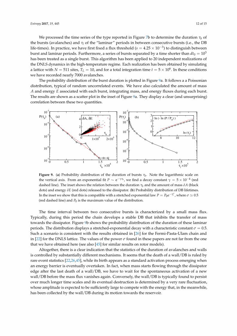
We processed the time series of the type reported in Figure 7b to determine the duration τb ofthe bursts (avalanches) and τl of the “laminar” periods in between consecutive bursts (i.e., the DBlife-times). In practice, we have first fixed a flux threshold (s = 4.25× 10−3) to distinguish betweenburst and laminar periods. Furthermore, a series of bursts separated by a time shorter than dt0 = 103

has been treated as a single burst. This algorithm has been applied to 20 independent realizations ofthe DNLS dynamics in the high-temperature regime. Each realization has been obtained by simulatinga lattice with N = 511 sites, TL = 10, and for a total integration time t = 5× 106. In these conditionswe have recorded nearly 7000 avalanches.

The probability distribution of the burst duration is plotted in Figure 9a. It follows a a Poissoniandistribution, typical of random uncorrelated events. We have also calculated the amount of massA and energy E associated with each burst, integrating mass, and energy fluxes during each burst.The results are shown as a scatter plot in the inset of Figure 9a. They display a clear (and unsurprising)correlation between these two quantities.

0 0.5 1 1.5 2

τb

×104

10-7

10-6

10-5

10-4

10-3

P(τb)

0 1×104

2×104

τb0

2

4 δA, δE(a)

0 0.5 1 1.5 2τ

l×10

5

10-8

10-7

10-6

10-5

10-4

10-3

P(τl)

8 10 12

ln (τl)0

1

2

3ln (- ln (P / P

0) )(b)

Figure 9. (a) Probability distribution of the duration of bursts τb. Note the logarithmic scale onthe vertical axis. From an exponential fit P ∼ e−γτb , we find a decay constant γ = 5× 10−4 (reddashed line). The inset shows the relation between the duration τb and the amount of mass δA (blackdots) and energy δE (red dots) released to the dissipator. (b) Probability distribution of DB lifetimes.In the inset we show that this is compatible with a stretched exponential law P = P0e−τσ

l , where σ ' 0.5(red dashed line) and P0 is the maximum value of the distribution.

The time interval between two consecutive bursts is characterized by a small mass flux.Typically, during this period the chain develops a stable DB that inhibits the transfer of masstowards the dissipator. Figure 9b shows the probability distribution of the duration of these laminarperiods. The distribution displays a stretched-exponential decay with a characteristic constant σ = 0.5.Such a scenario is consistent with the results obtained in [26] for the Fermi-Pasta-Ulam chain andin [22] for the DNLS lattice. The values of the power σ found in these papers are not far from the onethat we have obtained here (see also [45] for similar results on rotor models).

Altogether, there is a clear indication that the statistics of the duration of avalanches and wallsis controlled by substantially different mechanisms. It seems that the death of a wall/DB is ruled byrare event statistics [22,26,45], while its birth appears as a standard activation process emerging whenan energy barrier is eventually overtaken. In fact, when mass starts flowing through the dissipatoredge after the last death of a wall/DB, we have to wait for the spontaneous activation of a newwall/DB before the mass flux vanishes again. Conversely, the wall/DB is typically found to persistover much longer time scales and its eventual destruction is determined by a very rare fluctuation,whose amplitude is expected to be sufficiently large to compete with the energy that, in the meanwhile,has been collected by the wall/DB during its motion towards the reservoir.

Entropy 2017, 19, 445 13 of 15

6. Conclusions

We have investigated the behavior of a discrete nonlinear Schrödinger equation sandwichedbetween a heat reservoir and a mass/energy dissipator. Two different regimes have been identifiedupon changing the temperature TL of the heat reservoir, while keeping fixed the properties ofthe dissipator. For low TL and low chemical potential, a smooth β-profile is observed, whichextends (in the central part) to negative temperatures without, however, being accompanied bythe formation of discrete breathers over the time scales accessible to numerical simulations. In the lightof the theoretical achievements by Rumpf [17–20], the negative-temperature regions are incompatiblewith the assumption of local thermodynamic equilibrium, which instead appears to be satisfied inthe positive-temperature part. Therefore, despite the smoothness of the profiles and the stationarityof mass and energy fluxes, such negative-temperature configurations should be better consideredas metastable states. Unfortunately, it is not easy to investigate this regime; no single heat bath canimpose a fixed negative T in a meaningful way so as to be able to compare with equilibrium states.It is therefore necessary to simulate larger systems in the hope to observe the spontaneous formationof breathers, the only obvious signature of negative temperatures. We plan to undertake such a kind ofnumerical studies in the near future. It is nevertheless remarkable to see that negative temperaturesare steadily sustained for moderately long chain lengths. As a second anomaly, we report the slowdecrease of the mass-flux with the chain length: the hallmark of an unconventional type of transport.This feature is, however, not entirely new; a similar scenario has been previously observed in setupswith dissipative boundary conditions and no fluctuations [42].

For larger temperatures TL, we observe an intermittent regime characterized by the alternation ofinsulating and conducting states, triggered by the appearance/disappearance of discrete breathers.Note that this regime is rather unusual, since it is generated by increasing the amount of energyprovided by the heat bath rather than by decreasing the chemical potential, as observed for example inthe superfluid/Mott insulator transition in Bose-Einstein condensates in optical lattices. Although,for clarity, we referred to the low and high TL cases, there is no special difference to be expected in theintermediate regime, except for the typical timescale for DB creation that may be, still, exceedinglylarge. In fact, for finite N, such a timescale becomes much shorter above some typical TL.

The intermittent presence of a DB/wall makes the chain to behave as a rarely leaking pipe, whichreleases mass droplets at random times when the DB disappears according to a stretched-exponentialdistribution. The resulting fluctuations of the fluxes suggest that the regime is stationary but notsteady, i.e., locally the chain irregularly oscillates among different macroscopic states characterized,at best, by different values of the thermodynamic variables. A similar scenario is encountered in the XYchain, when both reservoirs are characterized by a purely dissipation accompanied by a deterministicforcing [42]. In such a setup, as discussed in Reference [42], the temperature in the middle of the chainfluctuates over macroscopic scales. Here, however, given the rapidity of changes induced by the DBdynamics, there may be no well-defined values of the thermodynamic observables. For example,during an avalanche it is unlikely that temperature and chemical potentials are well-defined quantities,as there may not even be a local equilibrium. This extremely anomalous behavior is likely to smear outin the thermodynamic limit, since the breather life-time does not probably increase with the systemsize, however, it is definitely clear that the associated fluctuations strongly affect moderately-longDNLS chains.

Acknowledgments: This research did not receive any funding. Stefano Lepri acknowledges hospitality of theInstitut Henri Poincaré-Centre Emile Borel during the trimester Stochastic Dynamics Out of Equilibrium wherepart of this work was elaborated.

Author Contributions: Stefano Iubini performed the numerical simulations. All Authors contributed to theresearch work and to writing the paper.

Conflicts of Interest: The authors declare no conflict of interest.

Entropy 2017, 19, 445 14 of 15

Abbreviations

The following abbreviations are used in this manuscript:

DNLS Discrete Nonlinear SchrödingerDB Discrete Breather

References

1. Lepri, S.; Livi, R.; Politi, A. Thermal conduction in classical low-dimensional lattices. Phys. Rep. 2003,377, 1–80.

2. Dhar, A. Heat Transport in low-dimensional systems. Adv. Phys. 2008, 57, 457–537.3. Basile, G.; Delfini, L.; Lepri, S.; Livi, R.; Olla, S.; Politi, A. Anomalous transport and relaxation in classical

one-dimensional models. Eur. Phys J. Spec. Top. 2007, 151, 85–93.4. Eilbeck, J.C.; Lomdahl, P.S.; Scott, A.C. The discrete self-trapping equation. Physica D 1985, 16, 318–338.5. Eilbeck, J.C.; Johansson, M. The Discrete Nonlinear Schrödinger Equation-20 Years on; World Scientific:

Singapore, 2003.6. Kevrekidis, P.G. The Discrete Nonlinear Schrödinger Equation; Springer: Berlin/Heidelberg, Germany, 2009.7. Scott, A. Nonlinear Science. Emergence and Dynamics of Coherent Structures; Oxford University Press: Oxford,

UK, 2003.8. Kosevich, A.M.; Mamalui, M.A. Linear and nonlinear vibrations and waves in optical or acoustic

superlattices (photonic or phonon crystals). J. Exp. Theor. Phys. 2002, 95, 777.9. Hennig, D.; Tsironis, G. Wave transmission in nonlinear lattices. Phys. Rep. 1999, 307, 333–432.10. Franzosi, R.; Livi, R.; Oppo, G.; Politi, A. Discrete breathers in Bose–Einstein condensates. Nonlinearity

2011, 24, R89.11. Rasmussen, K.; Cretegny, T.; Kevrekidis, P.G.; Grønbech-Jensen, N. Statistical mechanics of a discrete

nonlinear system. Phys. Rev. Lett. 2000, 84, 3740–3743.12. Franzosi, R. Microcanonical Entropy and Dynamical Measure of Temperature for Systems with Two First

Integrals. J. Stat. Phys. 2011, 143, 824–830.13. Iubini, S.; Lepri, S.; Politi, A. Nonequilibrium discrete nonlinear Schrödinger equation. Phys. Rev. E 2012,

86, 011108.14. Sievers, A.; Takeno, S. Intrinsic localized modes in anharmonic crystals. Phys. Rev. Lett. 1988, 61, 970.15. MacKay, R.; Aubry, S. Proof of existence of breathers for time-reversible or Hamiltonian networks of

weakly coupled oscillators. Nonlinearity 1994, 7, 1623.16. Flach, S.; Gorbach, A.V. Discrete breathers—Advances in theory and applications. Phys. Rep. 2008, 467, 1–116.17. Rumpf, B. Simple statistical explanation for the localization of energy in nonlinear lattices with two

conserved quantities. Phys. Rev. E 2004, 69, 016618.18. Rumpf, B. Transition behavior of the discrete nonlinear Schrödinger equation. Phys. Rev. E 2008, 77, 036606.19. Rumpf, B. Stable and metastable states and the formation and destruction of breathers in the discrete

nonlinear Schrödinger equation. Phys. D Nonlinear Phenom. 2009, 238, 2067–2077.20. Rumpf, B. Growth and erosion of a discrete breather interacting with Rayleigh-Jeans distributed phonons.

Europhys. Lett. 2007, 78, 26001.21. Iubini, S.; Franzosi, R.; Livi, R.; Oppo, G.; Politi, A. Discrete breathers and negative-temperature states.

New J. Phys. 2013, 15, 023032.22. Livi, R.; Franzosi, R.; Oppo, G.L. Self-localization of Bose-Einstein condensates in optical lattices via

boundary dissipation. Phys. Rev. Lett. 2006, 97, 60401.23. Franzosi, R.; Livi, R.; Oppo, G.L. Probing the dynamics of Bose–Einstein condensates via boundary

dissipation. J. Phys. B At. Mol. Opt. Phys. 2007, 40, 1195.24. Tsironis, G.; Aubry, S. Slow relaxation phenomena induced by breathers in nonlinear lattices. Phys. Rev. Lett.

1996, 77, 5225.25. Piazza, F.; Lepri, S.; Livi, R. Slow energy relaxation and localization in 1D lattices. J. Phys. A Math. Gen.

2001, 34, 9803.26. Piazza, F.; Lepri, S.; Livi, R. Cooling nonlinear lattices toward energy localization. Chaos 2003, 13, 637–645.

Entropy 2017, 19, 445 15 of 15

27. Reigada, R.; Sarmiento, A.; Lindenberg, K. Breathers and thermal relaxation in Fermi–Pasta–Ulam arrays.Chaos 2003, 13, 646–656.

28. De Roeck, W.; Huveneers, F. Asymptotic localization of energy in nondisordered oscillator chains.Commun. Pure Appl. Math. 2015, 68, 1532–1568.

29. Cuneo, N.; Eckmann, J.P. Non-equilibrium steady states for chains of four rotors. Commun. Math. Phys.2016, 345, 185–221.

30. Oikonomou, T.; Nergis, A.; Lazarides, N.; Tsironis, G. Stochastic metastability by spontaneous localisation.Chaos Solitons Fractals 2014, 69, 228–232.

31. Geniet, F.; Leon, J. Energy transmission in the forbidden band gap of a nonlinear chain. Phys. Rev. Lett.2002, 89, 134102.

32. Maniadis, P.; Kopidakis, G.; Aubry, S. Energy dissipation threshold and self-induced transparency insystems with discrete breathers. Phys. D Nonlinear Phenom. 2006, 216, 121–135.

33. Johansson, M.; Kopidakis, G.; Lepri, S.; Aubry, S. Transmission thresholds in time-periodically drivennonlinear disordered systems. Europhys. Lett. 2009, 86, 10009.

34. Iubini, S.; Lepri, S.; Livi, R.; Politi, A. Off-equilibrium Langevin dynamics of the discrete nonlinearSchroedinger chain. J. Stat. Mech Theory Exp. 2013, 2013, P08017 .

35. Borlenghi, S.; Iubini, S.; Lepri, S.; Chico, J.; Bergqvist, L.; Delin, A.; Fransson, J. Energy and magnetizationtransport in nonequilibrium macrospin systems. Phys. Rev. E 2015, 92, 012116.

36. Kulkarni, M.; Huse, D.A.; Spohn, H. Fluctuating hydrodynamics for a discrete Gross-Pitaevskii equation:Mapping onto the Kardar-Parisi-Zhang universality class. Phys. Rev. A 2015, 92, 043612.

37. Mendl, C.B.; Spohn, H. Low temperature dynamics of the one-dimensional discrete nonlinear Schroedingerequation. J. Stat. Mech Theory Exp. 2015, 2015, P08028.

38. Yoshida, H. Construction of higher order symplectic integrators. Phys. Lett. A 1990, 150, 262–268.39. Rugh, H.H. Dynamical approach to temperature. Phys. Rev. Lett. 1997, 78, 772.40. Iacobucci, A.; Legoll, F.; Olla, S.; Stoltz, G. Negative thermal conductivity of chains of rotors with

mechanical forcing. Phys. Rev. E 2011, 84, 061108.41. Ke, P.; Zheng, Z.G. Dynamics of rotator chain with dissipative boundary. Front. Phys. 2014, 9, 511–518.42. Iubini, S.; Lepri, S.; Livi, R.; Politi, A. Boundary-induced instabilities in coupled oscillators. Phys. Rev. Lett.

2014, 112, 134101.43. Iubini, S.; Lepri, S.; Livi, R.; Politi, A. Coupled transport in rotor models. New J. Phys. 2016, 18, 083023.44. Ng, G.; Hennig, H.; Fleischmann, R.; Kottos, T.; Geisel, T. Avalanches of Bose–Einstein condensates in

leaking optical lattices. New J. Phys. 2009, 11, 073045.45. Eleftheriou, M.; Lepri, S.; Livi, R.; Piazza, F. Stretched-exponential relaxation in arrays of coupled rotators.

Phys. D Nonlinear Phenom. 2005, 204, 230–239.

c© 2017 by the authors. Licensee MDPI, Basel, Switzerland. This article is an open accessarticle distributed under the terms and conditions of the Creative Commons Attribution(CC BY) license (http://creativecommons.org/licenses/by/4.0/).