a chance-constrained approach for electric vehicle ... · electric vehicle aggregator participation...

FACULDADE DE ENGENHARIA DA UNIVERSIDADE DO PORTO

A Chance-Constrained Approach forElectric Vehicle Aggregator

Participation in the Reserve Market

António Sérgio Barbosa Faria

Mestrado Integrado em Engenharia Eletrotécnica e de Computadores

Supervisor: Professor Manuel António Cerqueira da Costa Matos

Co-Supervisor: Tiago Soares, PhD

Co-Supervisor: Tiago Sousa, PhD

July 17, 2019

c© António Sérgio Barbosa Faria, 2019

Abstract

Increasing environmental concerns have led to changes in the power system, and the investmentin distributed energy resources is in progress. However, the investment in renewable energy isusually associated to the intermittent behavior of the energy sources, like the sun, wind, waves,etc. In the last decade, Electric Vehicles (EV) have been continuously rising, and the trend isto play an important role in the power system. Thus, new relationships between EVs and marketagents shall be addressed. Nowadays, EVs already have the ability to charge and discharge energy,known as Vehicle-to-Grid mode (V2G). This feature aided by proper algorithms, can contribute tothe frequency and voltage support of the network. It all depends on the willingness of the vehicleowner to provide this type of services, always ensuring minimum State-Of-Charge (SOC) for thedaily trips. Generally, the management of the electrical system is associated with high powerlevels, so EVs should be aggregated in order to be able to engage in this type of service. Thus, theconcept of EV aggregator arises.

The EV aggregator concept entails joining several EVs together so they can actively participatein energy and ancillary services markets. This aggregator should gather all the information relatedto the fleet and relate to the market agents. Through operational algorithms, the EV aggregatorshould be able to achieve their goals benefiting all those involved.

This thesis proposes a optimization model for solving the EV aggregator problem, consideringthe uncertainty and risk associated to the EVs usage for reserve provision. The proposed modelincludes penalties in the event of a failure in the provision of upward or downward reserve. There-fore, stochastic and chance-constrained programming are used to handle the uncertainty of a smallfleet of EVs and the risk behavior of the EV aggregator. Chance-constrained optimization throughthe deterministic equivalent (including Big-M and McCormcik relaxation methods) are appliedin order to assess the risk of the EV aggregator decision. The proposed model is applied underthe rules of the Frequency-Controlled Normal Operation Reserve (FCR-N) in East Denmark. It isimplemented on a small fleet of 10 EVs from the Frederiskberg Forsyning utility company withinthe scope of the PARKER project. This methodology also presents two different probabilities ofconnecting the EVs to the network, considering different availability to provide the service, whichmay be related to poor connections.

Finally, the proposed model is validated and tested for different numbers of scenarios anddifferent risk levels. Regarding the two methods discussed, Big-M and McCormick, they presentvery similar results when taking into account the aggregator’s profit. The McCormick methodpresents a slightly better performance when the number of scenarios increases, which indicatesits greater usefulness in large scale problems. However, it also presents the setback of requiringa greater computational effort. The probability functions also have a significant impact on theexpected profit of the EV aggregator. An out-of-sample approach is also considered, assessing theoutcomes of the aggregator’s decision.

i

Resumo

As crescentes preocupações ambientais têm levado a alterações no sistema de energia, e por isso,é necessário haver investimento em recursos energéticos distribuídos. Contudo, o investimentonesta área está normalmente associado a energia solar, eólica, das ondas, etc. Na última década,os veículos elétricos têm-se desenvolvido e a tendência é que possam desempenhar um papelimportante no sistema de energia. Por isso, é importante que sejam desenvolvidas novas relaçõesentre os agentes de mercado e os EVs. Atualmente, os EVs já têm capacidade para carregar edescarregar energia (V2G). Esta funcionalidade, suportada pelos algoritmos certos pode contribuirpara ajudar a rede elétrica a mitigar problemas de tensão e frequência. Tudo está dependente dadisponibilidade dos proprietários dos EVs, sendo que a carga necessária para as suas viagensdiárias será sempre assegurada. Geralmente, o controlo do sistema de energia está associado aelevados níveis de potência, por isso os EVs devem aglomerar-se para terem a possibilidade deprestar auxílio. Deste modo, nasce o conceito de agregador de EVs.

O conceito de agregador de EVs envolve associar vários EVs para que eles consigam miti-gar problemas na rede, uma vez que já têm uma capacidade significativa. Este agregador devereunir informação relativa a toda a frota e relacionar-se com os agentes de mercado. Através dealgoritmos operacionais, o agregador de EVs deve atingir os seus objetivos e beneficiar todos osenvolvidos. Esta tese propõe um novo modelo de otimização para resolver o problema que o agre-gador de EVs suscita para fornecer reserva, uma vez que há incerteza e risco associados. O modeloproposto inclui penalidades caso não seja fornecida reserva a subir e a descer. Assim, otimizaçãoestocástica e chance-constrained são utilizadas para tratar de incerteza e risco associados ao prob-lema. Os métodos de relaxação Big-M e McCormick são aplicados de modo a analisar o risco que oagregador submete em mercado. O modelo é implementado numa pequena frota de 10 veículos dacompanhia Frederiskberg Forsyning, no âmbito do projeto PARKER. Esta metodologia tambémapresenta duas probabilidades diferentes da conexão do EV à rede, que representam diferentesdisponibilidades para fornecer o serviço, que podem estar relacionadas com más conexões. Final-mente, o modelo proposto é validado e testado para diferentes números de cenários e diferentesníveis de risco. Relativamente as dois métodos analisados, Big-M e McCormick, os resultadosapresentados são semelhantes, quando se tem em consideração o lucro do agregador. Para ummaior número de cenários, o método McCormick apresenta uma ligeira melhor performance, oque é um indicador que esta método apresenta uma melhor resposta em problemas reais. Contudo,este método também exige um maior tempo computacional. As funções de probabilidade tambémapresentam um elevado impacto no lucro do agregador. São também gerados outros cenários paraavaliar a resposta do agregador.

iii

Acknowledgments

First of all, I would like to thank my parents for everything they have done for me and for puttingmy studies first. It is not easy to have a life of sacrifice so I can have one with better conditions,so to them goes my greatest gratitude.

Secondly, I would like to thank my brother for his companionship and closeness. For alwaysbeing present and for supporting me.

To thank the supervisors Manuel Matos, Tiago Soares and Tiago Sousa. Without them it wouldnot have been possible. They had an important impact on all opinions and certainly improved mycritical spirit. Special thanks to Tiago Soares for all his patience and incredible willingness to helpme whenever necessary.

Last but not least, to highlight all the people who have accompanied me along this journey.Thank António for all his help and availability whenever I needed it. To all the friends who haveaccompanied me along this journey, my many thanks, for making this task much more enjoyable.

António Sérgio Barbosa Faria

v

“Design is not how it looks like and feels like.Design is how it works”

Steve Jobs

vii

Contents

1 Introduction 11.1 Context . . . . . . . . . . . . . . . . . . . . . . . . . . . . . . . . . . . . . . . 11.2 Objetives . . . . . . . . . . . . . . . . . . . . . . . . . . . . . . . . . . . . . . 21.3 Thesis Structure . . . . . . . . . . . . . . . . . . . . . . . . . . . . . . . . . . . 3

2 EV Aggregator Overview 52.1 EV Aggregator . . . . . . . . . . . . . . . . . . . . . . . . . . . . . . . . . . . 5

2.1.1 Vehicle-to-Grid . . . . . . . . . . . . . . . . . . . . . . . . . . . . . . . 62.1.2 Distribution System Operator (DSO) and Transmission System Operator

(TSO) Interaction and Electricity Market . . . . . . . . . . . . . . . . . 62.1.3 Economic Value of V2G . . . . . . . . . . . . . . . . . . . . . . . . . . 7

2.2 Electricity Markets . . . . . . . . . . . . . . . . . . . . . . . . . . . . . . . . . 72.2.1 TSO . . . . . . . . . . . . . . . . . . . . . . . . . . . . . . . . . . . . . 72.2.2 Market Schemes . . . . . . . . . . . . . . . . . . . . . . . . . . . . . . 82.2.3 Ancillary Services . . . . . . . . . . . . . . . . . . . . . . . . . . . . . 8

2.3 Optimization and Control Algorithms . . . . . . . . . . . . . . . . . . . . . . . 112.3.1 Strategic Offering . . . . . . . . . . . . . . . . . . . . . . . . . . . . . . 112.3.2 EVs Energy Scheduling . . . . . . . . . . . . . . . . . . . . . . . . . . 142.3.3 Operation and Control of EVs in the Network . . . . . . . . . . . . . . . 152.3.4 Overview of Optimization and Control Algorithms . . . . . . . . . . . . 15

3 EV Aggregator Market Model 173.1 Architecture . . . . . . . . . . . . . . . . . . . . . . . . . . . . . . . . . . . . . 173.2 Offering Strategy Through Chance-Constrained Approach . . . . . . . . . . . . 19

3.2.1 Big-M Method . . . . . . . . . . . . . . . . . . . . . . . . . . . . . . . 193.2.2 McCormick Envelopes . . . . . . . . . . . . . . . . . . . . . . . . . . . 20

3.3 Problem Description and Mathematical Formulation . . . . . . . . . . . . . . . . 213.4 Bilinear Reformulation of the Chance-Constrained Problem . . . . . . . . . . . . 23

4 Case Study 274.1 Data Description . . . . . . . . . . . . . . . . . . . . . . . . . . . . . . . . . . 274.2 Computational Tools . . . . . . . . . . . . . . . . . . . . . . . . . . . . . . . . 294.3 Big-M vs. McCormick . . . . . . . . . . . . . . . . . . . . . . . . . . . . . . . 31

4.3.1 Expected Profit Analysis . . . . . . . . . . . . . . . . . . . . . . . . . . 314.3.2 Computational Effort . . . . . . . . . . . . . . . . . . . . . . . . . . . . 344.3.3 Best and Worst Case Scenarios . . . . . . . . . . . . . . . . . . . . . . . 36

4.4 Available and Plugged Probabilities Impact . . . . . . . . . . . . . . . . . . . . 374.5 One-week Simulation Results . . . . . . . . . . . . . . . . . . . . . . . . . . . . 38

ix

x CONTENTS

4.5.1 Expected Costs of Risk . . . . . . . . . . . . . . . . . . . . . . . . . . . 40

5 Conclusion and Future Work 435.1 General Contributions . . . . . . . . . . . . . . . . . . . . . . . . . . . . . . . . 435.2 Future Work . . . . . . . . . . . . . . . . . . . . . . . . . . . . . . . . . . . . . 44

A Appendix 47

References 49

List of Figures

3.1 Schematic structure of EV participation in ancillary services. . . . . . . . . . . . 183.2 Representation of McCormick Envelopes. . . . . . . . . . . . . . . . . . . . . . 20

4.1 Market Prices considered for one week. . . . . . . . . . . . . . . . . . . . . . . 284.2 Available probability vs. Plugged probability for one week. . . . . . . . . . . . . 294.3 TSO imbalance signal for one scenario . . . . . . . . . . . . . . . . . . . . . . . 294.4 MATLAB/GAMS information exchange. . . . . . . . . . . . . . . . . . . . . . 304.5 Expected profit by scenarios and risk level for the Big-M method applied to the

TSO balance constraint. . . . . . . . . . . . . . . . . . . . . . . . . . . . . . . . 324.6 Expected profit by scenarios and risk level for the Big-M method applied to the

SOC constraint. . . . . . . . . . . . . . . . . . . . . . . . . . . . . . . . . . . . 324.7 Expected profit by scenarios and risk level for the McCormick method applied to

the TSO balance constraint. . . . . . . . . . . . . . . . . . . . . . . . . . . . . . 334.8 Expected profit by scenarios and risk level for the Big-M method applied to the

TSO balance constraint under available probability . . . . . . . . . . . . . . . . 384.9 Neglected scenarios expected costs vs. Expected revenue. . . . . . . . . . . . . . 40

xi

xii LIST OF FIGURES

List of Tables

2.1 Overview of state of the art studies. . . . . . . . . . . . . . . . . . . . . . . . . 16

4.1 Electric vehicles characteristics. . . . . . . . . . . . . . . . . . . . . . . . . . . 274.2 Upward and downward offers characteristics. . . . . . . . . . . . . . . . . . . . 284.3 Computational effort under Big-M method (s). . . . . . . . . . . . . . . . . . . . 354.4 Computational effort under McCormick method (s). . . . . . . . . . . . . . . . 354.5 Computational effort for one-week simulation under Big-M method and 50 sce-

narios (s). . . . . . . . . . . . . . . . . . . . . . . . . . . . . . . . . . . . . . . 354.6 Computational effort for one-week simulation under McCormick method and 50

scenarios (s). . . . . . . . . . . . . . . . . . . . . . . . . . . . . . . . . . . . . 364.7 Best and worst case scenarios under Big-M method. . . . . . . . . . . . . . . . . 364.8 Best and worst case scenarios under McCormick method. . . . . . . . . . . . . . 374.9 Cumulative results of one-week simulation under the McCormick method. . . . . 39

A.1 GAMS model status codes. . . . . . . . . . . . . . . . . . . . . . . . . . . . . . 47A.2 Cumulative results of one-week simulation under Big-M method-Plugged proba-

bility . . . . . . . . . . . . . . . . . . . . . . . . . . . . . . . . . . . . . . . . . 48A.3 Cumulative results of one-week simulation under Big-M method-Available prob-

ability . . . . . . . . . . . . . . . . . . . . . . . . . . . . . . . . . . . . . . . . 48

xiii

xiv LIST OF TABLES

Abbreviations

DSO Distribution System OperatorEV Electric VehicleEDV Electric-Drive VehiclesFCR-D Frequency-Controlled Disturbance ReserveFCR-N Frequency-Controlled Normal Operation ReserveGHG Greenhouse GasGSM Global System ManagementLP Linear ProgrammingMINLP Mixed-Integer Nonlinear ProgrammingMIP Mixed-Integer ProgrammingPHEV Plug-in Hybrid Electric VehiclePSO Particle Swarm OptimizationSO System OperatorSOC State of ChargeTSO Transmission System OperatorV2G Vehicle-to-Grid

xv

xvi Abbreviations

Symbols

ParametersM Big-M parameterηCh Charge efficiencyηDch Discharge efficiencyπω Probability of scenario ω

π plugged Probability of the vehicle be plugged to the grid in time Γ

λ Prices and penaltiesλ sp Energy spot priceVariablesP Powerr Amount of reserve deployed in the second-stagerev RevenueR Amount of offered reserve in the first-stageRLXD Amount of power for missing offered downward reserveRLXU Amount of power for missing offered upward reserveSOC State-of-charge of the electric vehicle ev at the end of period tX Binary variable for charging/discharging selectionY Binary variable for offering in the marketSubscriptsω Scenario indexCh Charge processDch Discharge processev Electric vehicle indext Period indexSuperscriptsDA Day-ahead – first-stageDW Downward reserveE EnergyForecast Forecast estimation of EV’s tripMax Upper bound limitMin Lower bound limitpnlt Penalty for missing the contracted reserveRT Real-time – second-stageUP Upward reserve

xvii

Chapter 1

Introduction

1.1 Context

In the face of increasing environmental and social concerns, sustainable development is imperative

in every field in order to ensure that future generations are not compromised. Particularly in the

area of energy where significant changes are already underway in developed and in developing

countries, however, there is a long way to go, especially for the whole planet. The constant emis-

sions of Greenhouse Gas (GHG) are one of the biggest scourges of today, which can be mitigated

by investing in energy from renewable sources and energy efficiency measures.

According to a study by the European Environment Agency [1], in 2016, the transport sector

accounted for 27% of GHG emissions. On the same year, emissions from transport increased

by 26% compared to 1990, which dictates that they should decrease by 2/3 by 2050 in order to

comply with the decrease defined in the Transport White Paper [2].

In this context, electric vehicles can play an important role as long as they are supported by an

electric power system, essentially made up of clean energy. The technology of these vehicles is

continuously evolving and they are now able to compete with vehicles that use fossil fuels. With

the penetration of EVs there is also a decrease in external dependence on energy, hence there are

several government supports to encourage the use of this type of transport.

Given the likelihood of high percentages of EV penetration in the future, it is also impera-

tive to study the impacts it may imply on the electric power system. The concept of Smart Grid

already encompasses the accentuated presence of EVs. Hence, the need to improve the infrastruc-

ture of the power system arises, in order to be prepared for this upcoming reality. Increases in

load levels, congestion and voltage variations are expected, so it is mandatory to develop control

and automation infrastructures. The charging of EVs should be scheduled smartly to avoid grid

overloading during peak hours and to benefit from off-peak hours charging. When the charging

schedule is not properly performed, many benefits that EVs can bring to the grid are being lost,

namely if high GHG emission power plants are dispatched. If EVs work as flexible loads they

can contribute to balancing power in the grid, as they have faster responses times and batteries

1

2 Introduction

can store energy cheaper than conventional methods. EVs can also act as a resource through V2G

capability, injecting power back to the grid to mitigate voltage or frequency fluctuations.

Domestic consumers and EVs lack the capacity to enter the market directly. Therefore, a way

for them to engage is to relate through aggregators. By then, they will be able to participate in the

market with a significant level of power. Therefore, energy aggregators are concepts that are being

implemented in various sectors, using technological advances. The role of the typical consumer

has been changing over time, so the aggregators have the ability to create value that can benefit the

entire power system. However, there are still many doubts and discussions around how to integrate

these aggregators and who should benefit most from their integration.

As expected, the concept of aggregator arises in EVs as well. So, these aggregators are new

market players who have to compete with each other and have the capability to attract new con-

sumers. It is an agent that interacts with the System Operator (SO), controlling the charging

process according to the momentary needs of the system. From the point of view of the system

operator the aggregator is seen as a part of the control architecture. From the aggregator’s point of

view, it functions as a flexible load with storage capacity that can deliver energy at a lower price

than that purchased or provide ancillary services.

The EV aggregator is responsible for gathering a set of information on the EVs’ characteris-

tics and on the users’ characteristics. All this information is handled and from this point on the

aggregator is available to interact with the different market agents. The EV aggregator must di-

rectly optimize the charging process of each EV. The EV aggregator uses operation management

algorithms, in order to decrease forecast errors in the many uncertainties that this problem en-

compasses and to achieve the optimal bidding strategy. Regarding the main objective of the EV

aggregator, it may vary and may be to increase its own profits, to benefit the network or to decrease

GHG emissions. The option should be suitable and the profits should be applied to attract more

customers.

1.2 Objetives

The power system’s stability strongly depends of its ability to adapt and how it is managed. The

increasing penetration of EVs can lead to small differences in the way energy is managed in the

different markets of each country. As the role of the EV aggregator is still under development, it is

important to exploit it so that its implementation achieves the best results and benefits to all those

involved. Thus, the objectives of this thesis are:

• Analyze the state of the art in order to identify the already developed concepts of EVs

aggregator and their applied problems;

• Adapt the strategic offering model for an EV aggregator participation in the reserve market

proposed in [3], by applying chance-constrained programming. This modeling will allow

the aggregator to have a trade-off between solution reliability and expected profit;

• Compare two different ways to apply chance-constrained: Big-M and McCormick methods;

1.3 Thesis Structure 3

• Exploring different probability distribution functions of EVs being connected to the grid,

and ready or not to provide the service;

• Assessment of proposed approaches through a real case study, comprising the comparison

of expected profit, offering strategy and computational effort.

1.3 Thesis Structure

This thesis is divided into 5 chapters, structured as follows:

• Chapter 1, the present one, depicts the contextualization of the problem and the main objec-

tives to be achieved;

• Chapter 2 presents an overview of the EV aggregator, namely the different definitions and

the application of this concept. It also presents the interactions between the different market

agents and the aggregator. A brief reference to the electricity markets is introduced, focus-

ing on ancillary optimization. Finally, an analysis is made of several existing control and

optimization algorithms;

• Chapter 3 details the offering strategy problem, accounting for the relations between the

market agents and the aggregator. The model proposed and implemented in this thesis are

described. The mathematical formulation of the strategic offering problem with chance-

constrained programming is presented. All the mathematical formulation for the reformula-

tion of the equivalent deterministic problem through the Big-M and McCormick methods is

exposed;

• Chapter 4 describes the realistic case study used to assess the proposed model. The perfor-

mance of the proposed model is presented and analyzed;

• Chapter 5 gathers the most important conclusions and proposes some future work that can

be developed in the area.

4 Introduction

Chapter 2

EV Aggregator Overview

This chapter provides an overview of the EV aggregator concept. Different forms of interaction

with the system will be analysed, as well as different options that the aggregator can offer for

participating in the energy market. Some general concepts about the energy market will also

be discussed, essentially concerning the reserve market. Finally, the existing literature will be

reviewed, namely several algorithms that optimize the integration of EV aggregators in the power

system.

2.1 EV Aggregator

EVs have storage and power capabilities with economic value, which can be aggregated, and

therefore improve profits [4]. Current market rules, do not allow small-size power resources to

participate in the market [5], which means that EV owners should look for aggregators.

The aggregator participates in short-term power market, namely day-ahead and real time, sub-

mitting forward regulation offers. The charging process is controlled by the aggregator according

to the implemented algorithm, and in return, the EV owner receives attractive tariffs and shares

the profits [6].

Another work [7] supports that EV aggregator works like an intermediary between the EVs

and the SO, therefore, it needs to know every information on the EV, which can be provided in an

online database. All that information, combined with historical data, should be enough to forecast

with some certainty the available capacity at any point. This allows the aggregator participating in

the market with high confidence levels, thus reducing penalties for energy not supplied.

Recent works [8] introduce the same concept, but aiming to maximize flexibility of EV’s

batteries. It does not not consider them as conventional loads but as mobile batteries, containing

information about the owners behaviour. These batteries should be charged with slow/medium

rates since it reduces their degradation, reduce power flow and increase charging duration which

gives more flexibility to the SO. They also claim that EVs should be charged in different locals as

smart households, buildings and parking lots, controlled by smart meters, allowing money savings

5

6 EV Aggregator Overview

to the EVs owners. Thus, EVs penetration, new business opportunities can be promoted and SO

can increase system’s efficiency, as well.

2.1.1 Vehicle-to-Grid

EVs can be seen as reliable energy sources, that can interact with the system or associated as an

aggregator. The concept of Electric-Drive Vehicles (EDV) includes two different classes, namely:

battery vehicles and hybrids. Hybrids also comprises plug-in and fuel-cell. All those EVs are

equipped with power electronics allowing them to discharge energy into the grid, i.e., supporting

frequency grid services. Specialists consider that EVs should play an important role in energy

systems, whereas ancillary services appear as the most profitable one [9].

The V2G definition assumes that every EV, while parked, can provide ancillary services. To

this end, it should be guaranteed: grid connection, control systems to communicate with the SO

and have smart meters. Thus, the SO can require energy when needed [10]. EVs industry has been

developed which means that it might play an important role in the power system, however its main

purpose should not be left aside, ensure enough energy for the trips.

2.1.2 Distribution System Operator (DSO) and Transmission System Operator (TSO)Interaction and Electricity Market

The EV aggregator is seen by the DSO as an agent of the market, which can have a fundamental

role on the grid operation when needed. To the TSO, aggregators are seen as possible source

to provide ancillary services [11]. Thereby, the interaction between these three agents works as

follows:

• In the beginning of each market session the aggregator buys electric energy to charge bat-

teries;

• DSO validates and corrects, if necessary, aggregators offer, always concerning technical

limits of the system. This correction should be seen as a revenue, leading to the inevitability

of new ways of management and market rules.

• TSO defines the needs for the next hours or days. From now one, the aggregator makes

its decision to participate or not in the market, having the possibility of profit through the

adjustment of the charging tariff.

All this process requires communications systems between the three market agents, that should

be bidirectional. The charging schedule and energy flow should be provided from the EV aggre-

gator to the system operators (DSO and TSO), as discharging schedule and charging interruptions

should be provided to the aggregators by the SOs [11]. Hereupon, are needed some mechanisms

as [12]:

• A human interface capable of showing to the costumers, in real time, the power flow and

information on maintenance and interruptions;

2.2 Electricity Markets 7

• Basic smart meters, to support SO management as well to aware the consumer about his

consumption in every moment;

• Information storage, in order to maintain historical data to create consumption patterns and

quality of service indicators;

• EV should be able to establish communications with the infrastructure in an autonomous

way;

• Failure communication, as charging process will be dependent of communication infras-

tructures. In case a failure occurs the charging process must continue in a non-optimized

way, ensuring EV owner’s trip.

2.1.3 Economic Value of V2G

Financial opportunities of V2G vary according to the market, the EV type and other characteristics

to provide the service. EVs can store energy, charge in valley hours and discharge in peak hours.

It can also provide ancillary services, namely, upward and downward regulation and spinning

reserve, always taking in account the impact it causes in the battery [9]. In Singapore, a study have

showed that the storage capacity can improve around 50 MW only with a 2% EVs penetration, or

more if the driver behaviour is known [13]. The same study states that V2G profit can be offered

as encouragement to spread EVs penetration.

Another investigation [14] conducted in the California reserve market (CAISO), over a period

of three years, shows the capabilities an aggregator can have. The results show that profits between

US$150,000 and US$2.1 million can be achieved by providing upward and downward regulation.

2.2 Electricity Markets

The reformulation of the relation between producer and consumer identities led to the introduc-

tion of the electricity markets, whereas the concept pool market raised, which include short-term

mechanisms aiming to balance the consumption and the production according to the offers made

by the producers or the consumers. Usually, this kind of market works in the previous day to

which it is implemented, being known as day-ahead market. The coordination of the technical

operation is normally ensured by the TSO, involving the exchange of information with producers

and market operators [15].

2.2.1 TSO

TSOs are entities that operate independently from other players in the market, such as generat-

ing companies, traders, suppliers, distributors and directly connected costumers. The TSO gives

access to the grid to these players, who are obliged to comply with the rules it imposes. The se-

curity of the energy supply is also ensured by the TSO in order to ensure a good functioning of

the system. In some countries the TSO is also responsible for grid infrastructure development and


maintenance. As these processes entail high costs, usually the TSO is a monopoly. The TSO is in

charge of transmitting the electrical power from the power plants to the regional or local distribu-

tion operators. One of the most important factors when it comes to energy transport is to ensure

the reliability of the process, which is why the TSO are interconnected regionally or nationally.

The roles of the TSO in the entire electricity market include managing the security of the power

system in real time and coordination between generation and load.

All TSOs are required to maintain a continuous, second-by-second, balance between elec-

tricity supply from power stations and demand from consumers and also ensure the provision of

reserves that will allow for sudden contingencies. This is achieved through an optimal economic

dispatch, according to the load. Any abnormal event is handled through sophisticated communi-

cation and modelling systems [16].

2.2.2 Market Schemes

The market is assembled in different schemes, namely, baseload power, peak power, spinning

reserve and regulation, which differ in control methods, response time, duration and prices [10]:

• Baseload power, is typical, sold in long term contracts and several studies have shown that it

is not the best choice to the EV aggregator since it have low storage capacities, short average

lifetime and high costs, being its advantages quick response and availability [17] [10].

• Peak power, is considered when high load levels are reached and, in general, is supported

by generators with high capacity [10].

• Spinning reserve is related to the capacity of quick generation. Typically, in this service, the

generators are connected and synchronized to the grid and are spinning in partial velocities,

so that in case of abnormal events occur they can respond quickly. This service get revenue

for the amount of time it is available, even if it is not used, which is ideal for EVs that are

connected to the grid, regularly [10].

• Regulation, it is crucial for the electrical system to keep the voltage and frequency in its

reference values, which implies that generation and loads are balanced. If the generation is

higher than loads then the system frequency will raise, if load is higher than generation, fre-

quency will decrease. All these aspects bring the inevitability of quick response generation

or flexible loads ready to reduce or cut its consumption. Thus, upward reserve assumes the

existence of generation units ready to increase the supplied power or loads ready to reduce

its consumption. On the other hand, downward reserve assumes the existence of generation

units ready to reduce its supplied power, or loads ready to increase its consumption [18].

2.2.3 Ancillary Services

It is important to balance demand and supply, in and near real time, even after markets have closed

(gate closure). Therefore, it is important that this process is guaranteed at the lowest cost and

2.2 Electricity Markets 9

ideally with environmental benefits, reducing the need to activate other energy sources. Usually,

TSOs are responsible for contracting this type of service and should have the capacity to: black

start, frequency response, fast reserve, provision of reactive power, among others. Access to these

resources can come from various sources, and it is preferable to do so, as it increases TSO’s

flexibility. These sources can be generators, but also costumers who can change their operating

patterns to help balance the system [19]. Typically, three frequency control types are considered:

• Primary control: it is an automatic control that quickly adjusts active power and load values,

aiming to stabilize the frequency. Its main purpose is to level the frequency when a large

generation or load outages occur [18] [20].

• Secondary control: adjusts active power to restore frequency and interchanges with other

systems after an imbalance. As primary control limits and avoids frequency variations,

secondary control restore the frequency value. Secondary control is not mandatory, therefore

some systems dismiss it [18] [20].

• Tertiary control: usually is enabled by the TSO and concerns a manual adjust in the genera-

tion in order to balance primary and secondary reserves, and deal with interchange problems.

It also works as a complement to the secondary control, in large generation or load outages

[18] [20].

2.2.3.1 The Portuguese Case

Portugal is under the Continental Europe power system, and therefore, it follows the rules of this

power system. In more detail, the frequency-control services are are commonly divided into three

different reserves, namely primary reserve, secondary reserve and regulation reserve [21]:

• Primary reserve is a mandatory and unpaid system service provided by the generators in

service and aims to automatically correct instantaneous imbalances between the production

and consumption. The resulting power variation shall be replaced within 15 seconds in the

event of disturbances that cause frequency deviations of less than 100 mHz and between 15

and 30 seconds for frequency deviations between 100 and 200 mHz.

• The proper operation of the electric power system, both from an economic point of view

and in terms of guaranteeing supply and safety of operation in the short and medium term,

requires a central regulator - frequency control. The achievement of these objectives shall be

ensured, as long as the technical limitations are respected, against deviations resulting from

random variations in consumption and against sudden imbalances between production and

consumption caused by the loss of generating units or sporadic deviations in consumption.

The Global System Management (GSM) is obliged to communicate to all market agents by

1 p.m. of each day the required secondary regulation reserve for each period of the following

day. It is necessary to establish the proportions between the upward and downward reserve

and the minimum secondary regulation band to be offered per offer. The communication of

the offers available to provide this service must take place between 6:00 p.m. and 6:45 p.m..


• The proper operation of the electric power system, both from an economic point of view

and in terms of guaranteeing supply and short and medium term operation safety requires

an additional active power reserve which ensure that consumption is covered and that the

system operates safely in the event of an incident that cause imbalances between generation

and consumption, capable of depleting both primary and secondary reserves. Market agents

shall be obliged to submit daily, within the limits of the the operation process an offer

with the entire regulation reserve available, both upward and downward, for the next day.

Immediately after the publication of the results of the secondary reserve, and until at 8:00

p.m. on the day prior to the date to which they refer, market agents shall provide to the GSM

the information relating to the reserve regulation. The reserve regulation offers shall respect

the maximum and minimum value limitations imposed by GSM following the technical

validation previously performed. In the event of non-compliance with the amount of the

contracted power, the deviations for a time period of 15 minutes shall be considered and

these deviations shall be accounted for and must be the responsibility of the market agent

that has not complied.

2.2.3.2 The Danish Case

Denmark is operating under the Continental Europe and Nordic power systems rules. Therefore,

the provision of ancillary services in Denmark depends on the geographical position and is divided

into DK1 (Continental Europe power system) and DK2 (Nordic power system). The operation of

ancillary services in DK1 follows similar rules as Portugal, since it belongs to the Continental

Europe power system. In the Nordic power system, ancillary services are operated and contracted

following different rules. The main ancillary services to be delivered in DK2 are [22]:

• The frequency-controlled normal operation reserve (FCR-N) is designed to maintain the

balance between production and consumption in order to keep the frequency close to 50

Hz. It consists of both upward and downward regulation and is provided by a symmetrical

reserve where both regulation reserves are procured together. The normal reserve supply

shall be activated each time the frequency deviates by +/- 100 mHz from the nominal value.

It must be activated within a maximum of 150 seconds and should be supplied linearly. The

supplier can submit hourly offers or block bids. Block bids submitted at the auction two

days before the day of operation (D-2) may have a duration of up to six hours. Block bids

submitted on the day before the operation day (D-1) may have a duration of up to three

hours. The player determines the hours at which the block bid starts, however the block bid

has to end on the same day of operation. Each bid has a minimum capacity of at least 0,3

MW and is always accepted in its entirely or not at all. For the availability payment to be

effected, the capacity must in fact be available. This means that the availability payment is

cancelled, and the player must cover any additional costs incurred in connection with cover

purchases.

2.3 Optimization and Control Algorithms 11

• Frequency-controlled disturbance reserve (FCR-D), exists to cover major system distur-

bances, so it needs to be fast for regulating the frequency following frequency drops re-

sulting from the outage of major production units. It is an automatic upward regulation

reserve provided by production or consumption facilities which respond to frequency de-

viations. This reserve activation is automatic in the event of drops to under 49.9 Hz and

remains active until the balance has been restored or the manual reserve takes over the sup-

ply of power. FCR-D must be able to supply non-inverse power at frequencies between 49.9

and 49.5 Hz, supply 50% of the response within 5 seconds and supply the remaining 50%

of the response within na additional 25 seconds. A delivery of this service can be made up

from several production or consumption units with different characteristics which together

can provide the service within the required response time. The procurement of this service

is made at daily auctions where part is procured two days before the operation day (D-2)

and part is procured one day before the operation day (D-1). As in FCR-N, the supplier can

submit bids hourly or as block bids and each one must be entered for a minimum of 0.3

MW. Bids are always accepted in their entirely or not at all.

• Manual reserve, which are also procured in DK1, is a manual upward and downward reg-

ulation reserve activated by the control entre. The reserve relieves the FCR-N in the event

of minor imbalances and ensures balance in the event of outages or restrictions affecting

production facilities and interconnections. These reserves are put up for sale at daily auc-

tions. Manual reserves are requested in DK1 and DK2 to meet the demand during individual

hours. The manual reserve is used to restore system balance and should be supplied within

15 minutes after the activation. An auction is held once a day for each of the hours of the

coming day of operation.

2.3 Optimization and Control Algorithms

In this section, it is intended to analyse algorithms regarding EVs integration and modelling, either

individually or as an aggregator. Different approaches are considered by several authors, some

give more prominence to the aggregator’s point of view as maximizing the profit, minimizing the

battery degradation, respecting minimum SOC levels, and other goals concerning the SO needs,

as the voltage control, minimizing losses, operational costs and GHG emissions.

2.3.1 Strategic Offering

In [3] a model is proposed for the participation of an EV aggregator in the reserve market, namely

the FCR-N in Denmark. The objective is to increase the aggregator’s profit from participating in

this type of service and takes into account possible penalties for noncompliance with the contracted

reserve provision. The strategic participation is modeled as a two-stage stochastic program. The

methodology studied considers both deterministic and stochastic approaches. This work also has

the particularity of considering different probabilities of connecting the EV to the grid, so it may


or may not be available to provide the service. The results show a better performance when the

stochastic methods are considered. It also proves that grid connection can have a big impact on

the aggregator’s profit, so investments in this field can generate profits and bring greater flexibility

to the aggregator.

Han [23] proposes a model to optimize charging variables to participate in reserve market,

through dynamic programming techniques. He assumes that the energy required for the next trip

is always above the current one, so charging is the only control element. Three variables are

assumed: charging sequence, charging duration and charging rate. If the SOC is given as a point

rather than as an interval, the charging duration problem is solved, and there is only one problem

with two variables. When formulating this optimization, the capacity of the batteries and their

weight were taken into account. Through the use of dynamic programming, optimal charging was

achieved for all vehicles, which were verified in simulation. This study is a strategic approach for

the V2G aggregator. Positive results were also achieved regarding the relationship between the

SOC and the revenues achieved.

Kristoffersen [24] defines an optimal charging model for an EV aggregator to participate in the

daily market of Nordpool, considering the driving patterns of the fleet and market prices fluctuation

through linear and quadratic programming. The goal is to charge the EV at a lower price, and then

sell it in V2G, if it pays off. Electricity costs, battery degradation and fuel costs are considered.

The results mainly suggest that EVs provide most of the flexibility only through charging, and

not by energy storing. It also points that charging process should occur during off-peak hours.

However, with a high EV penetration rate, it may raise higher peak loads at this hours, which

attenuates profits that the selling could bring.

In [25] the authors use an approach that involves fuzzy optimization in order to model the

uncertainties forecasted that occur in the electricity market, mainly prices. The results show the

benefits that the application of fuzzy algorithms can bring when compared to deterministic meth-

ods that do not consider the market uncertainties. The objective is to maximize the aggregator’s

revenue by participating in the regulation and spinning reserves market. Both models reduce peak

load charging tariffs. Regarding expected revenues, these vary according to the expected SOC,

but there is an agreement regarding the models with fuzzy algorithms, since the average profit is

always 2 or 3 times higher than expected with the deterministic models.

In [26] author presents a mathematical model for optimal charging and discharging, for spin-

ning reserve market participation. The authors state that EV owners should respect the EV ag-

gregator and not disconnect the EV earlier than planned. To solve the MINLP problem is used

a simulated annealing algorithm, in order to increase aggregator profit. The study concludes that

low spinning reserve and higher market prices reduce aggregator profit.

In [27], the authors bring forward an optimal bidding strategy of an EV aggregator in day-

ahead and reserve market, always considering the perfect forecast of day-ahead energy and regu-

lation prices. It was identified key sources of uncertainty and included in the model which aimed

to maximize the profit while providing reliable reserve levels. It concludes the aggregator has a

preference for offering downward regulation instead of upward regulation. Costs of EV charg-


ing can became profits when the aggregator gets involved in the reserve market and the way the

battery is charged is decisive to evaluate the true capability of the aggregator’s market partici-

pation. Ortega-Vasquez [28] proposes a similar model, however, it compensates EV owners for

battery degradation. It was implemented as a Mixed-Integer Programming (MIP) and guarantees

to the system operating cost savings from its participation in reserve markets. The results prove

the aggregator benefits from reserve more than the energy market as it obtains revenue for pro-

viding regulation without battery degradation. Furthermore, it affords a comparison with battery

costs in the future, expected to decrease, which will raise aggregator’s revenue and reduce system

operating costs.

In [29] is investigated the design and performance of a system that would enable EV ag-

gregator to participate in wholesale electricity markets including intraday and pay-as-bid reserve

markets that require exact reserve delivery and have long operating intervals. The main goal is

to maximize the reserve provision while making sure there are enough energy for the trips. It

brings forward new ideas for achieving control of flexible loads with uncertain behaviour subject

to restrictive rules, concluding that the more flexible markets became, the more profit aggregators

can get through EV charging.

In [30], the flexibility of EV aggregator charging is studied in order to avoid forecasting er-

rors. In this way, it is possible to participate in the reserve manual market. The aggregator has

direct control over the EVs charging, however in this work it is not considered the V2G mode,

the aggregator only provides reserve through the increase or decrease of the charging rate. The

objective function is the minimization of the total cost divided in three components: cost of pur-

chasing energy in the energy market, cost from charging EV with downward reserve and income

from reducing the consumption (upward reserve). The results show that the participation of the

aggregator in the reserve market may represent a reduction of its wholesale costs. The authors

suggest that this cost reduction may help to attract new customers or increase the profit from retail

activity.

In [31] it is proposed an risk-averse optimal bidding strategy of an EV aggregator in a fre-

quency regulation market, under the rules of CAISO. The objective is to determine the optimal

offer to be submitted in the market. The problem is formulated as Mixed-Integer Programming

(MIP) and takes into account the uncertainties in the price of energy and frequency regulation.

The objective function of this model also includes the degradation of the battery caused by the

provision of the service. The objective of the proposed methodology is to maximize the aggrega-

tor’s profits. The results prove that it is indeed possible to reduce battery degradation if the energy

dispatch is optimal.

In [32] it is proposed that an EV aggregator participates in the reserve market. This formulation

takes into account the uncertainty in the availability of EVs to provide the service. Optimum

load and price levels are also developed. Comparisons are also made between unidirectional and

bidirectional V2G. The results point to a slightly better performance of bidirectional V2G, however

this also implies higher costs and consequently higher risks. Furthermore, with the prediction of

EV saturation in the future, the authors recommend the use of unidirectional V2G.


2.3.2 EVs Energy Scheduling

In [33] the authors use a MIP, since linear and integer variables are introduced into the problem of

EV charging coordination in an unbalanced distribution network. The formulation was applied to

a distribution network, considering the limits in the magnitude of voltages and currents. It was also

assumed that the batteries should be charged in a certain period of time, the energy required by

the battery is known at the beginning of each period and that the EV had communication devices

that allowed the DSO to control the battery SOC. Tests have shown that this model has a reduced

error level and that approximations are acceptable, so the MIP can be applied to solve this type of

problem.

In [34] stochastic and deterministic methods for optimizing hybrid vehicle charging plug-in

are compared. The impacts that these extra loads imply on power losses and voltage deviations

are analyzed. Both winter load profiles and summer load profiles for whole days divided into

15 minutes intervals are studied in the Belgian electrical system, and all loads are considered

residential. Generally, the differences between the stochastic and deterministic losses are quite

small, which means that load forecasting errors do not have much influence on the losses. It is

possible to verify also a decrease of losses when the load is controlled, mainly due to the decrease

of power required in peak hours.

Other authors focus their work on developing stochastic models to simulate the availability

of EVs to provide services to the network [35]. Fluhr uses the Monte-Carlo method to create the

probability distribution of the EV trip. The results show that EVs are parked more than 90% of the

time, which makes it beneficial to build residential charging infrastructure. In [36] a technique for

the sustainable integration of PHEVs is proposed, considering the most significant uncertainties.

Robust optimization is used in order to evaluate the risk levels of the introduction of Plug-in Hybrid

Electric Vehicles (PHEVs) in the transport sector. Others [37] use normal and Poisson distribution

to determine the probability of charging times and initial battery states. This work, performs case

studies to analyse intelligent charging algorithms for large amounts of PHEVs using Monte Carlo

method.

Sundstrom and Binding [38] describe a model to minimize charging costs and achieve satis-

factory SOC levels through deterministic methods. They compare linear and quadratic approxi-

mations to represent battery behaviour. The results indicate that linear approximation is sufficient

when the focus is on optimizing the charging schedule. Battery limit violations are always less

than 2% of their capacity when linear approximation is used, so the computational effort used by

quadratic approximation is not justified.

In [39] a modified model of Particle Swarm Optimization (PSO) is presented to solve the prob-

lem that high penetration of distributed generation and EVs raises, with the possibility of V2G.

The aim is to reduce operating costs. The optimization consists in the inclusion of mechanisms

that adjust the speed limits during the search process, thereby becoming more independent. The

authors argue that it has greater robustness, faster convergence and greater ability to deal with

constraints when compared to the PSO, which gives it the ability to solve large-scale problems ef-


ficiently. A real network is the target of study. With the increase in penetration there is also a huge

increase in computational execution time with with the deterministic method, which is a MINLP

model. With 2000 EVs, the deterministic method took about 25 hours to obtain the solution, while

the modified PSO presented a solution in 36 seconds, where the cost is only 1% higher than the

deterministic method.

An information gap decision theory is proposed in [40] to manage revenue risk of the aggre-

gator, due to the gap between the forecast and the real electricity prices. The model guarantees

a profit for risk-averse decision makers and for risk-seeking decision makers, where travel be-

haviours are simulated using the Monte Carlo method. The decision maker can choose between

robustness and opportunity functions based on the risk he is willing to take on the market.

2.3.3 Operation and Control of EVs in the Network

Sundstrom and Binding [41] describe basic aggregator’s functions regarding optimization prob-

lems, considering grid constraints as voltages and power flow. An individual charging schedule

is defined for each vehicle, in order to avoid distribution grid congestion. Two essential variables

are considered, namely the forecast of minimum energy for the next trip and the moment it will

happen. It is assumed that the information might be inaccurate, leading to prudent approaches,

guaranteeing error margins. Linear programming is used to characterize SOC and to formulate the

charging process, finding the optimal solution that minimizes battery charge. This model present

disadvantages and limitations: error margins may not be the solution that minimizes cost, since

high penalties will be applied; this method handles individual EV loads and does not act as an

aggregator that could reduce forecasting errors; it is also necessary to predict arrival time, which

introduces computational complexity [42].

Rotering and Ilic [43] propose and discuss the problem that EV charging can cause during

peak hours, in particular, overloads. Two algorithms are analysed based on predicting future

electricity costs and using dynamic programming to find the optimal solution for the EV owner.

Both algorithms consider that the forecast is ideal for both the EV variables and the demand

for reserve. The first optimizes charging time and energy flow, with the intention to reduce the

daily cost of electricity without damaging the battery. The second also takes into account the

support that the EV can give to the grid, always taking into consideration the technical constraints

of the grid, by participating in ancillary services, namely in the secondary reserve market. The

proposed models are implemented under the rules of CAISO. The results shows that smart charge

timing reduces daily electricity costs for driving from $0.43 to $0.2. It also states that provision of

regulating power improves PHEV economics.

2.3.4 Overview of Optimization and Control Algorithms

The table 2.1 summarises the information from the previous sections. The most important one

was considered such as the problem that the authors intend to solve, the main objective of the

optimization and the class on which the proposed methodology is based.


Table 2.1: Overview of state of the art studies.

Ref. Problem Objective Problem Class[3] Strategic Offering Maximize aggregator’s profit Stochastic and deterministic methods

[23] Strategic Offering Maximize aggregator’s profit Stochastic method[24] Strategic Offering Minimize total operation costs Analytical method[25] Strategic Offering Maximize aggregator’s profit Stochastic method[26] Strategic Offering Maximize aggregator’s profit Metaheuristic method

[27] Strategic OfferingMaximize aggregator’s profit and

reliable reserve provisionStochastic method

[28] Strategic OfferingMaximize aggregator’s profitwithout battery degradation

Stochastic method

[29] Strategic Offering Maximize reserve provision Metaheuristic method[30] Strategic Offering Minimization of the total cost Analytical method[31] Strategic Offering Maximize aggregator’s profit Stochastic method[32] Strategic Offering Maximize aggregator’s profit Deterministic method

[33] EVs Energy SchedulingMinimize the energy cost of EV

chargingStochastic method

[34] EVs Energy Scheduling Minimize the power losses Stochastic and deterministic methods[35] EVs Energy Scheduling Define Evs availability Stochastic method

[36] EVs Energy SchedulingMinimize the present value

of the net electricityand emission costs

Deterministic method

[37] EVs Energy SchedulingOptimally allocate the power

energy to PHEVsStochastic method

[38] EVs Energy Scheduling Minimize charging costs Deterministic method[39] EVs Energy Scheduling Minimize operation costs Metaheuristic and deterministic method[40] EVs Energy Scheduling Manage the revenue risk of the Analytical method

[41]Operation and Controlof EVs in the Network

Avoid distribution gridcongestion

Stochastic method

[43]

Strategic Offering,Evs Energy Scheduling,Operation and Controlof Evs in the Network

Optimizing the charging timeand energy flows;

Maximize aggregator’s profitAnalytical method

Chapter 3

EV Aggregator Market Model

This chapter details the strategic offering problem. The relationship between the aggregator and

the market agents is assessed. It also describes the model proposed and implemented regarding the

mathematical formulation of the problem with chance-constrained programming. In addition, it

also exposes the reformulation of the problem by the deterministic equivalent through the Big-M

and McCormick methods.

3.1 Architecture

An aggregator has the ability to control a set of EVs, i.e., it directly controls the charging patterns

of EVs promoting smart charging. The vehicles only need an interface to provide information such

as: SOC, EV type, power and battery capacity, charging characteristics and departure time. Thus,

the energy required for the next trip is ensured within a time interval, giving to the EV aggregator

the possibility to take control in the charging process during this period.

The TSO seeks to balance generation and load, and maintain frequency at nominal values, and

EVs are a potential provider of these services as they are flexible and have quick response times. It

would be a complex task if the TSO receives information from hundreds of thousands of vehicles,

so communication should be bi-directional. As depicted in Figure 3.1: to make this relationship

work, information must be exchanged between the aggregator and the EV. Thus, the EV should

provide information on consumption, EV status, SOC, EV type, battery capacity, power capacity

and charging characteristics. A communication between the aggregator and the TSO is also re-

quired, namely to inform about the balancing signal, seeling bid and market prices. Therefore, the

aggregator is able to gather all this information and make its participation in the reserve market as

effective as possible, increasing profits.

The TSO sends a signal of the reserve imbalance to the aggregator at each point in time, and

the aggregator handles this information and distributes the necessary energy to the vehicles that

are willing to provide the service in that period. Afterwards, the aggregator is able to predict the

available energy to meet the TSO requirement, and therefore informing the TSO by offering in the

market.

17

18 EV Aggregator Market Model

Figure 3.1: Schematic structure of EV participation in ancillary services.

The aggregator responds to TSO requests by participating in the ancillary services market. The

TSO is responsible for the system services market and selects the best offers from aggregators.

Thereafter, the aggregators activate the EVs so they can respond to the TSO signal. The bi-

directional charging will allow the vehicles to adjust according to the aggregator requests imposed

by the TSO, allowing them to provide upward and downward regulation. In return, the EV owner

is economically compensated. The EVs owners’ firm contract with the aggregator that offers better

tariff. The aggregator works as an electricity retailer, representing EVs drivers in the electricity

market, allowing to split the electricity price for this purpose and the inclusion of taxes from the

government [42].

The aggregator aims to manage the fleet of EVs taking into account the individual needs of

each vehicle, optimizing its bidding strategy in the reserve market. The aggregator operates as a

price-taker, i.e. it accepts prevailing prices in the market and cannot influence or dictate its prices.

This concept focuses on the needs of the aggregator, but it can also be extended and seen from the

point of view of the EV individually.

It is important to consider that the main purpose of the EV remains to ensure the normal travel

of users and only then to provide reserve services. Despite the evolution of the methods used to

forecast drivers’ behaviour and the existing databases, this prediction is always a complicated task

and will remain subject to errors, so the only uncertainty of this problem is the energy trip. The

SOC and the probability that the EV is plugged to the grid are considered parameters. In this way,

it is possible to formulate the problem stochastically, since there is randomness present. In order

to represent this randomness, a set of variables values are defined with a certain deviation, positive

or negative, and then an equal probability is applied to them. In doing so, more possibilities

will be covered and the response that the aggregator can provide will be better. This leads to the

implementation of the chance-constrained approach, which is one of the ways of analyzing the

risk of strategic offerings, considering uncertainty.

3.2 Offering Strategy Through Chance-Constrained Approach 19

3.2 Offering Strategy Through Chance-Constrained Approach

One of the biggest current challenges is related to the resolution of large-scale problems, the

chance-constrained method is one of the biggest approaches used in stochastic optimization prob-

lems, with a high uncertainty level. Essentially, it constrains a number of more unlikely scenarios,

so that the decision-maker can choose the level of reliability and risk that wishes and considers to

be adequate. Usually, this type of solution is robust, but in real dimension problems it can become

difficult to solve. The usual formulation for this type of problem is as follows:

min f (x,ξ ) (3.1)

s.t:

g(x,ξ ) = 0 (3.2)

h(x,ξ )≥ 0 (3.3)

where x is the decision vector, ξ is the uncertainty vector, g represents the equality constraints and

h the inequality constraints. Applying the chance-constrained method, the equality constraint is

represented as [44]:

P(g(x,ξ ) = 0)≥ 1− ε (3.4)

where ε represents the the risk to be defined by the decision-maker.

The chance-constrained programming is solved in several different ways. One of the solutions

may involve reformulation and resolution by the equivalent deterministic problem. This problem

can be derived through the Big-M method or through bilinear reformulation. Within the Big-M

method, a binary variable is used indicating whether the associated scenario should be considered

or may be violated, and thus the problem is converted into an MIP. Within the bilinear reformula-

tion approach, the constraint becomes bilinear, which is a particular case of nonlinear constraints.

Therefore, the McCormick relaxation method is used to relax the nonlinear constraint, turning it

convex and linear [45].

3.2.1 Big-M Method

Equation 3.4 can be converted through the Big-M method as follows:

−Mz(t,ω) ≤ g(x,ξ )≤Mz(t,ω), ∀ t ∈ T ;∀ω ∈Ω (3.5)

Ω

∑ω

π(t,ω)z(t,ω) ≤ ε,z(t,ω) ∈ 0,1 , ∀ t ∈ T (3.6)

where z(t,ω) represents the binary variable representing whether or not the scenario is active; M

represents the Big-M parameter, which should be sufficiently large; ε represents the pre-defined

risk, defined by the decision-maker.


3.2.2 McCormick Envelopes

The McCormick envelopes is a technique used to relax non-convex and non-linear functions using

the boundaries of the variables. This relaxation can find solutions faster and with less computa-

tional effort, however the solution is not the optima of the original problem. It is important to

choose a relaxation that has tightest bounds, in order to have limits that are closer to the ideal

solution [46]. This relaxation consists of setting up four linear lines that create an approximate

solution space to the function space, as depicted in figure 3.2.

Considering a bilinear function w=xy, then the relaxation of function w is given by:

w≥ xLy+ xyL− xLyL (3.7)

w≥ xU y+ xyU − xU yU (3.8)

w≤ xU y+ xyL− xU yL (3.9)

w≤ xyU + xLy− xLyU (3.10)

where xU and yU are the upper bounds for x and y; xL and yL are the lower bounds for x and y,

respectively. The equations 3.7 and 3.8 represent underestimators and 3.9 and 3.10 overestimators.

Figure 3.2: Representation of McCormick Envelopes.

3.3 Problem Description and Mathematical Formulation 21

3.3 Problem Description and Mathematical Formulation

This work focuses on the participation of an electric vehicle aggregator in the reserve market,

namely in FCR-N in Eastern Denmark, according to the rules of the Nordic power system, where

symmetric offering for upward and downward reserve is considered, as in [3]. This study considers

the uncertainty in the energy trip and consequently in the SOC. It also features the particularity

of modeling the probabilities of EVs being connected, but for some reason not being able to

provide the service, for example due to misconnections or other reasons, and the probabilities

being plugged-in and available to provide the service. The goal is to maximize the aggregator’s

profit by participating in the reserve market at day-ahead stage, taking into account that it can

suffer penalties for energy not supplied in real-time stage.

The main objective is to maximize the profit EV aggregator gets by participating in the FCR-N.

The strategic offering problem of the EV aggregator is modelled as a two-stage stochastic chance-

constrained problem. The first-stage includes the optimal reserve bid to offer in the reserve market,

and the second-stage models the activation of reserve and its associated imbalance costs. Thus,

the objective function to be maximized is presented in 3.11, and combines the revenues at the day-

ahead and real-time stages. The real-time stage considers the expected costs of failing to provide

the service.

maxrevDA + revRT (3.11)

The day-ahead stage is given by the capacity payment λ of upward and downward reserve

offered by the aggregator, in each time step t, as in 3.12

revDA =T

∑t=1

(λ

UPt RUP

t +λDWt RDW

t)

(3.12)

Real-time stage remuneration takes into account revenues for service activation and penalties

for reserve supply failures, both upward and downward, as can be seen in 3.13. It includes RLXU

and RLXD variables that represent the amount of power that was not provided for the ω scenario

of the Ω set, but was offered in the day-ahead. The discharge of energy is assumed zero, because

this study does not consider the participation in the energy service.

(3.13)revRT =

T

∑t=1

Ω

∑ω=1

πω

[−λ

UP,pnltt RLXU(t,ω) − λ

DW,pnltt RLXD(t,ω) + λ

spt

EV

∑ev=1

(PEDch(ev,t,ω)

− PECh(ev,t,ω) + PUP

Dch(ev,t,ω) + PUPCh(ev,t,ω))− PDW

Dch(ev,t,ω) − PDWCh(ev,t,ω))

]

The objective function is subject to several constraints related to technical limitations from the

first-stage, second-stage and from the way aggregator can use each vehicle.

Equations 3.14 and 3.15 limit the upward and downward power that the aggregator can provide

in the reserve service. This equation includes a binary variable stating whether the aggregator is


willing to participate in the reserve market at each time step. It cannot be higher than the total

capacity of the entire fleet or lower than a certain minimum.

PUP,MinYt ≤ RUPt ≤ PUP,MaxYt ,∀t ∈ T (3.14)

PDW,MinYt ≤ RDWt ≤ PDW,MaxYt ,∀t ∈ T (3.15)

3.16 requires that the aggregator’s participation in the reserve market is symmetrical according

to FCR-N rules, i.e., upward and downward bids must have both the same value.

RUPt = RDW

t ,∀t ∈ T (3.16)

The constraints 3.17 and 3.18 limit the the activation of reserve in the second-stage according

to the offer made in the first-stage, for each t in any scenario.

rUP(t,ω) ≤ RUP

t ,∀t ∈ T ;∀ω ∈Ω (3.17)

rDW(t,ω) ≤ RDW

t ,∀t ∈ T ;∀ω ∈Ω (3.18)

The balance between the system’s needs and the availability of the aggregator to supply the

contracted upward and downward reserve is presented in equation 3.19. The value of the system

needs can be positive or negative and is dependent on the aggregator’s willingness to provide the

service at each time. The RLXU and RLXD variables represent the relaxation of the balancing

equation, in cases the power available in the EVs being insufficient to provide what aggregator

have promised at the day-ahead stage.

Pr(∆SI(t,ω)Yt=rDW(t,ω)−rUP

(t,ω)+RLXD(t,ω)−RLXU(t,ω),∀t∈T ;∀ω∈Ω )≥ 1− ε (3.19)

The equations 3.20 and 3.21 consider the availability of each vehicle for the activation of the

upward and downward reserve in each period t and scenario ω . The activation of the EVs can lead

to either increase or decrease the actual charging and discharging power of the EVs battery.

rUP(t,ω) =

EV

∑ev=1

πplugged(ev,t)

(PUP

Dch(ev,t,ω)+PUPCh(ev,t,ω)

), ∀ t ∈ T ;∀ω ∈Ω (3.20)

rDW(t,ω) =

EV

∑ev=1

πplugged(ev,t)

(PDW

Dch(ev,t,ω)+PDWCh(ev,t,ω)

), ∀ t ∈ T ;∀ω ∈Ω (3.21)

Equations 3.22 and 3.25 denote that each vehicle may not reduce its charging power in upward

service if it is not charging in the power service, nor reduce its discharging power if it is not

discharging in the power service. Equations 3.23 and 3.24 indicate that each vehicle has an upper

charging and discharging limit, according to its characteristics. It also states that the charging and

3.4 Bilinear Reformulation of the Chance-Constrained Problem 23

discharging ability of the EVs cannot occur at the same period t. That is, the EV cannot charge

and discharge in the same period, and this is controlled by the binary variable X.

PECh(ev,t,ω) ≥ PUP

Ch(ev,t,ω),∀t ∈ T ;∀ω ∈Ω;∀ev ∈ EV (3.22)

PECh(ev,t,ω)+PDW

Ch(ev,t,ω) ≤ PMaxCh(ev,t)

(1−X(ev,t,ω)

),∀t ∈ T ;∀ω ∈Ω;∀ev ∈ EV (3.23)

PEDch(ev,t,ω)+PUP

Dch(ev,t,ω) ≤ PMaxDch(ev,t)X(ev,t,ω),∀t ∈ T ;∀ω ∈Ω;∀ev ∈ EV (3.24)

PEDch(ev,t,ω) ≥ PDW

Dch(ev,t,ω)∀t ∈ T ;∀ω ∈Ω;∀ev ∈ EV (3.25)

In addition, the SOC of each vehicle is determined in 3.26. In this equation the previous SOC,

the energy of each trip and its participation in the reserve market is taken into account for each ω

scenario and each t time interval, accounting for the charging and discharging efficiency.

Pr(SOC(ev,t,ω) = SOC(ev,t−1,ω) − ETrip(ev,t,ω)+ ∆ tηCh(ev)

(PE

Ch(ev,t,ω) − PUPCh(ev,t,ω) + PDW

Ch(ev,t,ω)

)− ∆t

ηDch(ev)(PE

Dch(ev,t,ω) − PUPDch(ev,t,ω) + PDW

Dch(ev,t,ω))) ≤ 1− ε,∀t ∈ T ;∀ω ∈ Ω;∀ev ∈ EV

(3.26)

In 3.27 the upper and lower battery limits for each EV are set.

SOCMin(ev,t) ≤ SOC(ev,t,ω) ≤ SOCMax

(ev,t),∀t ∈ T ;∀ω ∈Ω;∀ev ∈ EV (3.27)

The constraint 3.28, illustrates the stochastic process that represents the energy for the trip of

each vehicle, and represents the only uncertainty in this model.

ETrip(ev,t,ω) = EForecastTrip(ev,t)+∆ETrip(ev,t,ω),∀t ∈ T ;∀ω ∈Ω;∀ev ∈ EV (3.28)

The equation 3.29 states that at the end of the simulated day the SOC of each vehicle must be

between 65 and 85% of the maximum SOC in order to ensure driving needs or market participation

in the next hour of the following day.

0.65SOCMax(ev,t) ≤ SOC(ev,t,ω) ≤ 0.85SOCMax

(ev,t), ∀ t→ end;∀ω ∈Ω;∀ev ∈ EV (3.29)

3.4 Bilinear Reformulation of the Chance-Constrained Problem

The reformulation of the chance-constrained problem through the deterministic equivalent can

be performed through the Big-M and McCormick approaches, as explained in the section 3.2.

Through the Big-M method, one can introduces a binary variable to the chance-constrained equa-

tions 3.19 and 3.26. Therefore, both 3.19 and 3.26 can be reformulated as follows [45]:


−Mz(t,ω) ≤−∆SI(t,ω)Yt + rDW(t,ω)− rUP

(t,ω)+RLXD(t,ω)−RLXU(t,ω) ≤Mz(t,ω), ∀ t ∈ T ;∀ω ∈Ω

(3.30)

−Mz(t,ω) ≤ −SOC(ev,t,ω) + SOC(ev,t−1,ω) − ETrip(ev,t,ω)+ ∆ tηCh(ev)

(PE

Ch(ev,t,ω) − PUPCh(ev,t,ω)

+ PDWDch(ev,t,ω)

)− ∆t

ηDch(ev)(PE

Dch(ev,t,ω) − PUPDch(ev,t,ω) + PDW

Dch(ev,t,ω)) ≤ Mz(t,ω),

∀t ∈ T ;∀ω ∈ Ω;∀ev ∈ EV(3.31)

Ω

∑ω

π(t,ω)z(t,ω) ≤ ε,z(t,ω) ∈ 0,1 , ∀ t ∈ T (3.32)

where z represents the binary variable. When z=0, the constraints 3.19 and 3.26 assume their

original form. When z=1, the same constraints are ignored, meaning that can be violated. For

good performance of this relaxation method, the Big-M parameter (M) should be large enough

[45]. Equation 3.33 is able to constrain the number of scenarios in which z will take the value 1,

based on the control parameter ε defined by the decision-maker. The use of the Big-M method is

usually associated with issues such as determining the M-parameter value, without compromising

the validity of the constraints. Usually it is also associated with a decrease in computational

efficiency, being linked to long times of computational effort.

Another approach of reformulating the chance-constrained problem is through the bilinear

reformulation [45]. Thus, equation 3.19 can be reformulated through

(−∆SI(t,ω)Yt + rDW(t,ω)− rUP

(t,ω)+RLXD(t,ω)−RLXU(t,ω))(1− z(t,ω)) = 0, ∀ t ∈ T ;∀ω ∈Ω (3.33)

Ω

∑ω

π(t,ω)z(t,ω) ≤ ε,z(t,ω) ∈ 0,1 , ∀ t ∈ T (3.34)

Here, the same logic is applied as for the Big-M method. When z=0 the restrictions 3.19 and

3.26 take their original form. When z=1 all constraint is multiplied by zero, thus becoming an

non-responsive scenario.

This reformulation makes the problem nonlinear, since equation 3.33 is a bilinear equation.

The bilinear equation can be linearized through the McCormick envelopes [46], where it is possible

to convert it back into an MIP. Therefore, equation 3.33 can be rewritten as:

(3.35)(−∆SI(t,ω)Yt + ∆SI(t,ω)Yt) + rDW(t,ω) −

˜rDW(t,ω) − rUP

(t,ω) +˜rUP

(t,ω) + RLXD(t,ω)

− ˜RLXD(t,ω) − RLXU(t,ω) + ˜RLXU(t,ω) = 0, ∀ t ∈ T ;∀ω ∈ Ω

where,

3.4 Bilinear Reformulation of the Chance-Constrained Problem 25

Yt = Ytz(t,ω) (3.36)

˜rDW(t,ω) = rDW

(t,ω)z(t,ω) (3.37)

˜rUP(t,ω) = rUP

(t,ω)z(t,ω); (3.38)

˜RLXD(t,ω) = RLXD(t,ω)z(t,ω); (3.39)

˜RLXU(t,ω) = RLXU(t,ω)z(t,ω); (3.40)

Each of the equations 3.36, 3.37, 3.38, 3.39 and 3.40 is linearized as in equations 3.7, 3.8, 3.9

and 3.10:

• Equation 3.36 is replaced by:

Yt ≥ 0 (3.41)

Yt ≥ Y maxz(t,ω)+Ytzmax−Y maxzmax (3.42)

Yt ≤ Y maxz(t,ω) (3.43)

Yt ≤ Yt (3.44)


˜rDW(t,ω) ≥ rDW,minz(t,ω) (3.45)

˜rDW(t,ω) ≥ rDW,maxz(t,ω)+ rDW

(t,ω)− rDW,max (3.46)

˜rDW(t,ω) ≤ rDW,maxz(t,ω) (3.47)

˜rDW(t,ω) ≤ rDW

(t,ω)+ rDW,minz(t,ω)− rDW,min (3.48)


˜rUP(t,ω) ≥ rUP,minz(t,ω) (3.49)

˜rUP(t,ω) ≥ rUP,maxz(t,ω)+ rUP

(t,ω)− rUP,max (3.50)

˜rUP(t,ω) ≤ rUP,maxz(t,ω) (3.51)

˜rUP(t,ω) ≤ rUP

(t,ω)+ rUP,minz(t,ω)− rUP,min (3.52)



˜RLXD(t,ω) ≥ RLXDmin(t,ω)z(t,ω) (3.53)

˜RLXD(t,ω) ≥ RLXDmaxz(t,ω)+RLXD(t,ω)−RLXDmax (3.54)

˜RLXDUP(t,ω) ≤ RLXDmaxz(t,ω) (3.55)

˜RLXD(t,ω) ≤ RLXD(t,ω)+RLXDminz(t,ω)−RLXDmin (3.56)


˜RLXU(t,ω) ≥ RLXUmin(t,ω)z(t,ω) (3.57)

˜RLXU(t,ω) ≥ RLXUmaxz(t,ω)+RLXU(t,ω)−RLXUmax (3.58)

˜RLXU(t,ω) ≤ RLXUmaxz(t,ω) (3.59)

˜RLXU(t,ω) ≤ RLXU(t,ω)+RLXUminz(t,ω)−RLXUmin (3.60)

Chapter 4

Case Study

This chapter presents the analysis of the methodology proposed in chapter 3. The aim is to analyze

the behavior of the proposed model considering a wide range of cases. These cases comprise a set

of simplified and complex studies covering different scenarios for the aggregator.

4.1 Data Description

The case study is based on a real case, comprising the fleet of EVs from the Frederiskberg Forsyn-

ing utility company within the scope of the PARKER project [47]. 10 EVs were considered,

namely Nissan e-NV200 vans. 10 ENEL V2G charging units were used to charge and discharge

the EVs. Each ENEL charging unit has a capacity of 10kW, with a total sum of 100 kW, which

already allows the participation of the aggregator in the reserve market.

Further information of the EVs is shown in the table 4.1.

Table 4.1: Electric vehicles characteristics.

Battery capacity (kWh) 21Minimun SOC level (kW) 6.3

Maximum charge/discharge (kW) 10Minimum charge/discharge (kW) 0

EV charge/discharge efficiency (%) 88

It is worth mentioning that the minimum SOC of each battery, for any period, was defined as

30% of its maximum capacity. The SOC of the last period for each EV of one-day simulation is

used as the previous state for the next day simulation, guaranteeing the continuity of the results.

In the table 4.2, it is possible to find information regarding market prices for energy, upward

and downward reserve, as well as upward and downward deficit penalties. These data were ob-

tained from Energinet.dk website [48] and are for the period from 1 to 31 January 2017 in East

Denmark. The penalties for lack of contracted reserves were assumed to be 100 times higher than

the upward and downward reserve prices. The figure 4.1 depicts these prices for the first week.

27

28 Case Study

Table 4.2: Upward and downward offers characteristics.

Electric Vehicle Aggregator Min Mean MaxPower offer limits (kW) 40 - 100Upward price (e/kW) 3.7 46.1 221.5

Downward price (e/kW) 3.7 40.4 108.5Spot price (e/kW) -6.3 33.9 117.1

Upward deficit penalty (e/kWh) 370 461 2215Downward deficit penalty (e/kWh) 370 404 1085

Figure 4.1: Market Prices considered for one week.

In this study, two distinct probabilities are considered for the connection to the grid by the EVs.

One represents the probability that the vehicle is connected to the grid, but may not be available to

provide the service, π plugged . The other, πavailable, represents the probability of the vehicle being

connected to the grid and ready to provide the service. Figure 4.2 illustrates the distribution of

these probabilities for the first week.

The TSO imbalance signal is the expected amount of power that the EV aggregator must

provide in each period in a given scenario. This signal is based on a normal distribution and

includes information on four months of upward and downward reserve provision, capturing the

needs trend in the Danish system. In figure 4.3 it is possible to observe this signal for a period of

one week. Regarding the parameter presented in equation 3.28, ∆ETrip(ev,t,ω), representing EV trip

deviation of each scenario, was also based on a normal random distribution.

4.2 Computational Tools 29

Figure 4.2: Available probability vs. Plugged probability for one week.

Figure 4.3: TSO imbalance signal for one scenario

4.2 Computational Tools

In order to apply the proposed models two computational tools were essentially used: MATrix

LABoratory (MATLAB) and General Algebraic Modeling System (GAMS).

MATLAB is a powerful numerical computing language. This software integrates comput-

ing, visualization and programming in a user-friendly environment, given that the problems and

solutions presented are in familiar mathematical notation [49].

30 Case Study

Within the scope of this thesis, MATLAB is used to handle the input data of the model, and

therefore connect it to GAMS.

GAMS is a high-level modeling system for mathematical optimization and programming. The

results, after the GAMS optimization, are sent to MATLAB where the data is also processed for

further analysis.

Although via MATLAB it is possible to perform the optimizations of the presented models,

GAMS was chosen as optimization tool, because of its advantages in solving optimization prob-

lems using stochastic methods compared with MATLAB. In the GAMS software, the CPLEX

solver has been used to solve the proposed MIP problem. In figure 4.4, is depicted the information

exchange between MATLAB and GAMS.

Figure 4.4: MATLAB/GAMS information exchange.

In MIP problems solving, with integer variables, CPLEX uses the branch and bound algorithm

that solves series of Linear Programming (LP) subproblems. The single MIP generates many other

small problems, even if the problem is small it can become computationally intensive and require

large amounts of physical memory. CPLEX can also offer the solving of an MIP in parallel in a

distributed computing environment that harnesses the power of multiple computers or of multiple

nodes inside a single computer to achieve better performance.

GAMS/CPLEX also uses the following options [50]:

• Option IterLim=x; Responsible for setting the limit number of iterations. The algorithm

will stop and pass the current solution to GAMS. CPLEX handles the iteration limit for

MIP problems differently than some other GAMS solvers. For MIP problems, controlling

the length of the solution run by limiting the execution time (ResLim) is preferable.

4.3 Big-M vs. McCormick 31

• Option ResLim = x; Sets the time limit in seconds. The algorithm will terminate and pass

on the current solution to GAMS.

• Option OptCA = x; Absolute optimality criterion for a MIP problem. The OptCA option

asks CPLEX to stop when|BP−BF |< OptCA

where BF is the objective function value of the current best integer solution while BP is the

best possible integer solution.

• Option OptCR = x; Relative optimality criterion for a MIP problem. Notice that CPLEX

uses a different definition than GAMS normally uses. The OptCR option asks CPLEX to

stop when

(|BP−BF |)/(1.0e−10+ |BF |)< OptCR

where BF is the objective function value of the current best integer solution while BP is the

best possible integer solution. The GAMS definition is:

(|BP−BF |)/(|BP|)< OptCR

Furthermore, GAMS also provides a model status code regarding the reached solution. These

codes can be seen in the table A.1

It is important to note that are only accepted solutions with the model status codes 1, 2 and 8.

4.3 Big-M vs. McCormick

In this section, it is intended to analyze the performance of the Big-M and McCormick methods,

considering the expected profit and computational effort.

4.3.1 Expected Profit Analysis

Here, are compared the profit that the aggregator expects to achieve under different scenarios

number ω and different pre-defined risk ε . Only one-day simulation and only plugged probability

were considered. For all simulations, it is defined the parameter M=1000, which is a sufficiently

large number.

Firstly, it is meant to analyze the expected profit under Big-M method applied to two different

chance-constraints, namely the TSO balance and SOC balance constraints. So, applying equations

3.30, 3.31 and 3.33 to the problem, the following results were obtained:

32 Case Study

Figure 4.5: Expected profit by scenarios and risk level for the Big-M method applied to the TSObalance constraint.

Figure 4.6: Expected profit by scenarios and risk level for the Big-M method applied to the SOCconstraint.

In general one can see that, Big-M method applied to the balance between system needs and

the availability of the aggregator to provide the contracted reserve (Figure 4.5) has higher expected

profits than when applied to the SOC equation (Figure 4.6). The difference between these values

tends to increase in proportion to the pre-defined risk and the number of scenarios.

For the same number of scenarios and for 0% of risk level (ε=0%) the objective function takes

the same values, according to the scenario, regardless of the constraint used. This is due to the

fact that the constraint is not yet active and the worst case scenarios are not being violated, so the


problem is being solved without risk of violating any scenario. There are cases where ε is not

large enough to remove scenarios, as happens under 5 scenarios where only with 20% of risk level

(ε=20%) the first scenario is violated. Except for these cases, the TSO constraint always presents

better expected results for the aggregator. When comparing the application of the method in the

TSO constraint to that of the SOC, the following is verified for 50 scenarios (ω=50):

• For 5% risk level (ε=5%), the expected profit decreased 48%;




This downward trend is also true for all other numbers of scenarios, so when the aggregator looks

for more flexibility in making the decision, it should decide to choose the TSO constraint, as it is

the one that will ensure the highest profits.

Applying the McCormick method to the TSO constraint, equations the results obtained were:

Figure 4.7: Expected profit by scenarios and risk level for the McCormick method applied to theTSO balance constraint.

When comparing the Big-M with McCormick methods, regarding the TSO constraint, the

results obtained are very similar. In fact, the follow happened:

For 5 scenarios (ω=5):

• For 0%, 5%, 10% and 15% risk level (ε=0%, ε=5%, ε=10% and ε=15%) no differences

were noted, since no scenarios are violated yet;

• For 20% risk level (ε=20%) the expected profit of the McCormick method is 0.0026% lower

than the Big-M method.

34 Case Study

For 10 scenarios (ω=10), no differences are verified, the two methods present the same ex-

pected profit.


• For 0% and 5% risk level (ε=0% and ε=5%) no differences were noted;

• For 10% and 15% risk level (ε=10% and ε=15%) the expected profit of the McCormick

method is 0.0001% higher than the Big-M method;

• For 20% risk level (ε=20%) no differences were noted.


• For 0% risk level (ε=0%) no differences were noted;

• For 5% risk level (ε=5%) the expected profit of the McCormick method is 0.015% lower

than the Big-M method;

• For 10% risk level (ε=10%) the expected profit of the McCormick method is 0.1143%

higher than the Big-M method;

• For 15% risk level (ε=15%) the expected profit of the McCormick method is 0.1018%

higher than the Big-M method;

• For 20% risk-level (ε=20%) the expected profit of McCormick method is 0.0293% lower

than the Big-M method;

In general the McCormick method presents a better performance, since there are more cases

where it presents a higher expected profit and in the cases where that happens this increase is much

higher than the cases in which the Big-M method performs better. The biggest differences are also

found for the largest number of scenarios, which may indicate that the McCormick method may

be a more effective solution to real dimension problems.

4.3.2 Computational Effort

In this kind of problem, in which the time that the aggregator has to submit a proposal is an

important factor, it is critical that a solution should be found even if it is not the optimal one.

To do so, algorithm runtime limits have been defined. The IterLim option was limited to 2

hours for the Big-M method and limited to 4 hours for the McCormick method. The McCormick

method requires more computational processing time, since it involves a linearization of bilinear

terms. Each bilinear term is linearized through 4 constraints, hence the increase in computational

effort. Also the absolute and relative optimality criterion were limited to 1E−10 (OptCA=1E−10

and OptCR=1E−10).

By observing the tables 4.3 and 4.4 it is possible to conclude that only for 5 scenarios the

algorithm is able to find the optimal solution (Model Status Code=1), while for all other scenario

numbers the time limit is reached, meaning that GAMS was not able to find the optimal solution,

but an integer solution is obtained (Model Status Code=8).


Table 4.3: Computational effort under Big-M method (s).

TSOω

5 10 25 500% 6,53 7202,43 7203,06 7218,465% 7,36 7201,81 7202,86 7219,88

ε 10% 7,15 7214,18 7202,27 7213,6315% 7,25 7259,65 7202,35 7209,0520% 30,53 7200,94 7202,23 7226,61

Table 4.4: Computational effort under McCormick method (s).

TSOω

5 10 25 500% 5,71 14401,59 14402,68 14444,975% 5,57 14402,47 14404,09 14407,13

ε 10% 6,00 14403,76 14402,97 14411,7615% 5,74 14403,32 14402,32 14429,1520% 32,43 14402,56 14402,51 14426,79

Looking now at the tables 4.5 and 4.6, which represent the methods behavior for one-week

simulation, it is possible to observe that for 50 scenarios (ω=50) and 0% risk level (ε=0%) GAMS

finds three optimal solutions. For day 7, the McCormick method finds a solution that takes 45%

longer than with the Big-M method. However, on the day 6, the McCormick method can also find

the optimal solution, which does not occur under the Big-M method.

Table 4.5: Computational effort for one-week simulation under Big-M method and 50 scenarios(s).

ε

0% 5% 10% 15% 20%1 7208,90 7206,31 7213,12 7206,86 7214,652 7244,00 7209,02 7209,58 7213,57 7203,833 7240,44 7221,58 7206,98 7230,87 7213,26

Day 4 7238,27 7212,60 7215,08 7213,54 7213,955 7223,92 7208,90 7205,63 7203,20 7206,086 7248,17 7240,84 7215,16 7214,99 7215,177 73,64 7256,63 7251,67 7251,04 7265,19

36 Case Study

Table 4.6: Computational effort for one-week simulation under McCormick method and 50 sce-narios (s).

ε

0% 5% 10% 15% 20%1 14428,99 14413,40 14421,02 14410,20 14412,052 14415,49 14409,69 14405,97 14409,67 14417,003 14463,35 14503,47 14439,93 14449,62 14452,46

Day 4 14540,09 14433,59 14427,91 14413,24 14448,275 14496,52 14411,51 14410,08 14408,04 14405,536 615,72 14435,73 14439,13 14423,79 14417,337 106,54 14481,22 14477,09 14507,27 14510,87

4.3.3 Best and Worst Case Scenarios

In the tables 4.7 and 4.8, it is possible to find the best and worst case scenarios for each studied

method.

Table 4.7: Best and worst case scenarios under Big-M method.

TSOω

5 10 25 500% min 79,91 -34,81 -194,18 -158,42

max 135,09 105,60 107,64 121,985% min 79,91 -34,81 -47,87 -203,03

max 135,09 105,60 171,37 180,93ε 10% min 79,91 28,44 0,47 -13,50

max 135,09 169,21 188,19 208,3815% min 79,91 28,44 71,50 69,14

max 135,09 169,21 207,85 208,3820% min 171,21 131,20 147,88 171,21

max 208,38 208,37 208,39 208,38

Observing the table 4.7 one would expect that when the number of scenarios holds and the pre-

defined risk increases, the maximum value would remain constant and the minimum value would

increase, because the worst case scenario would be neglected. However, this is not the reality in all

cases, since a computational time limit was established due to the aggregator’s demand to be able

to find the offer to submit in the market in appropriate time. In some cases this temporal limitation

forces the algorithm to stop before the optimal solution being achieved, and therefore returns the

best solution found until that moment, which is feasible but not the optimal. In this cases, integer

solutions were found (Model status code=8). Analyzing the example of 50 scenarios (ω=50), for

0% and 20% risk level (ε=0% and ε=20%) the minimum value with the superior pre-defined risk

is higher, which should not be verified. This is due to the fact that the method performs different

relaxation and as the optimal solution was not found, these values present such inconsistency.

4.4 Available and Plugged Probabilities Impact 37

Table 4.8: Best and worst case scenarios under McCormick method.

TSOω

5 10 25 500% min 79,91 -34,81 -194,18 -158,42

max 135,09 105,60 107,64 121,985% min 79,91 -34,81 -47,87 -203,03

max 135,09 105,60 171,37 180,93ε 10% min 79,91 28,44 0,47 -13,50

max 135,09 169,21 188,19 208,3815% min 79,91 28,44 71,50 69,14

max 135,09 169,21 207,85 208,3820% min 126,73 131,20 147,88 177,18

max 201,11 208,37 208,39 208,38

Comparing tables 4.7 and 4.8 it can be noticed that the two methods often have the same

maximum and minimum values. The biggest difference is for 5 scenarios (ω=5) and 20% risk

level (ε=20%), where the minimum value under the McCormick method is 35% lower and the

maximum value is 4% lower, which means that for 5 scenarios the Big-M method is tightening

the objective function values. On the other hand, for 50 scenarios (ω=50) and 20% risk level

(ε=20%), under the McCormick method the values are tighter, the minimum value is 3% higher,

which again reinforces the effectiveness of this method for larger problems.

4.4 Available and Plugged Probabilities Impact

In this section the aim is to analyze the impact that a possible failure in the connection of vehicles to

the network may affect the expected aggregator’s profit. For this purpose, the Available probability

pattern in the figure 4.2 was used in the Big-M method. The results obtained were as follows:

Comparing the figure 4.8 with the 4.5, the following differences are observed:

• For 5 scenarios (ω=5): no differences were noted.

• For 10 scenarios (ω=10):

– For 0% and 5% risk level (ε=0% and ε=5%) no differences were noted;

– For 10% and 15% risk level (ε=10% and ε=15%) the expected profit decreased 0.14%;

– For 20% risk level (ε=20%) the expected profit decreased 0.03%.


– For 0% risk level (ε=0%) no differences were noted;

– For 5% risk level (ε=5%) the expected profit decreased 0.29%;

– For 10% risk level ( ε=10%) the expected profit decreased 0.23%;

38 Case Study

Figure 4.8: Expected profit by scenarios and risk level for the Big-M method applied to the TSObalance constraint under available probability




– For 0% risk level (ε=0%) no differences were noted;





It is now possible to realize how the probability of vehicles being connected to the grid can

influence the profit expected by the aggregator. Since these values only cover one day, in the long

term they can imply a lot of associated costs, which leads to the conclusion that improvements in

the connections between the EVs and the grid can improve the flexibility of the aggregator.

4.5 One-week Simulation Results

For one-week simulation and 50 scenarios, it is intended to analyze in more detail the performance

of the aggregator regarding the contracted reserve and reserve activation, as well as expected

inflow, costs and revenue, from different perspectives.

The Forecast simulation is exactly the same as all the simulations that have been performed so

far, intending to represent a reserve prediction of the market needs taking into account their need

and response from the aggregator.

4.5 One-week Simulation Results 39

The Deployed simulation represents the hour-ahead simulation based on potential realization

scenarios and constrained by the forecast simulation results, i.e., a deterministic optimization per

realization scenario. After the forecast performed previously, it is assumed that the contracted

reserve is considered a parameter, which means that its values are considered fixed and no re-

laxations are made. From this point on, new scenarios with the same distribution are generated,

leading to a different scheduling of EVs and other variables. The aggregator does not have the

deployed information before making its decision. To do this analyze, the McCormick method and

plugged probability were chosen.

Table 4.9: Cumulative results of one-week simulation under the McCormick method.

ε

0% 5% 10% 15% 20%Forecast Deployed Forecast Deployed Forecast Deployed Forecast Deployed Forecast Deployed

ContractedUpward reserve (kW) 14100,00 14100,00 15400,00 15400,00 16200,00 16200,00 16400,00 16400,00 16600,00 16600,00

ContractedDownward reserve (kW) 14100,00 14100,00 15400,00 15400,00 16200,00 16200,00 16400,00 16400,00 16600,00 16600,00

Upwardactivation (kWh) 3620,54 3398,83 3639,02 3721,88 3324,09 3887,68 3008,75 3936,01 2540,96 3985,20

Downwardactivation (kWh) 3567,49 3417,70 3696,57 3721,14 3568,49 3931,80 3457,19 3977,05 3233,69 4023,36

Upward deficit- RLXU (kWh) 29,26 176,03 24,85 192,09 14,98 214,98 8,35 220,67 2,42 225,09

Downwarddeficit - RLXD (kWh) 28,11 28,67 23,82 40,47 12,47 53,65 8,36 58,53 4,43 67,70

Expectedinflow (e) 1206,01 1206,01 1324,26 1324,26 1398,40 1398,40 1416,76 1416,76 1441,14 1441,14

Expected costs(e) 233,13 829,35 205,99 959,41 120,40 1125,80 71,26 1175,17 27,76 1254,78

Expectedrevenue (e) 972,88 376,66 1118,27 364,85 1277,99 272,60 1345,50 241,59 1413,38 186,36

The table 4.9 shows that the contracted reserve increases as ε increases, since the worst case

scenarios are excluded and there is the possibility of a better scheduling by the EVs to participate

in the reserve market. The values of the upward and downward reserve are equal for the same ε

because the market under consideration is symmetrical. It is possible to verify that the expected

inflow is equal, for the same value of ε , whether it is Forecast or Deployed. The expected costs

are related to the deficit of supplied reserve.

Regarding expected revenue for the forecast, as predicted, it increases as the ε increases, since

the worst case scenarios are neglected. For Deployed, there is an opposite effect, i.e., the expected

revenue decreases as the ε increases. This is due to the imposed contracted reserve value, which is

fixed forcing the aggregator to comply and to adapt to this value for new scenarios. This sometimes

leads leads to a slight increase in the value of relaxation variables (RLXU and RLXD), which have

a negative influence on expected profit since the penalty considered here is 100 times higher than

the upward and downward balancing power prices, respectively. For the Forecast, one can also

note that:

• when the risk level (ε) varies from 0% to 5%, the expected profit increases 15%;




40 Case Study

For the Deployed:

• when the risk level (ε) varies from 0% to 5%, the expected profit decreases 3%;




This information can also be useful to the aggregator because it establishes a trade-off regard-

ing the decision to be made.

4.5.1 Expected Costs of Risk

Typically, in this type of problem, the main objective is to maximize the expected profit. However,

the objective function is related to costs, and a reduction of this value can lead to an increase in

expected revenue. Risk exists in every field and is inevitable, so it is important for the aggregator

to quantify the existing risk and then be able to minimize or manage it. The aggregator must accept

responsibility for the attitude it has taken towards the risk.

Thus, it was calculated the costs that the neglected scenarios present, that is, the costs that they

represent for the aggregator when the binary variable z(t,ω) is active.

Figure 4.9: Neglected scenarios expected costs vs. Expected revenue.

Analyzing the figure 4.9, one can see that the costs of neglected scenarios increase along with

the expected revenue. As expected revenue increases with the pre-defined risk, as predicted, these

costs are increasing steadily. When the expected profit is higher than 1300e the slope becomes

even more accentuated, highlighting the ever-increasing costs that the aggregator is subject to.

The more scenarios the aggregator ignores, the greater will be the expected revenue in Forecast.

4.5 One-week Simulation Results 41

However, if these ignored scenarios occur, they entail higher costs. Therefore, it is important that

the decision maker takes into account this trade-off between expected revenue and the potential

costs of neglected scenarios.

42 Case Study

Chapter 5

Conclusion and Future Work

5.1 General Contributions

In the near future, EVs will change the current paradigm of energy markets, as they will play a key

role, especially, in ancillary services. Ancillary services are important to maintain and control the

stability of power systems. The most effective way for EVs to participate in this type of service

is through aggregators. These aggregators collect the most important and necessary information

and then relate to the TSO in order to optimize the offer made in the market. This offer can have

different objectives such as improving the profit of the aggregator, improving the profit of each

individual EV, providing the best service to the network, reducing the emission of GHG, etc.

This dissertation focuses on modeling the strategic offering of an EV aggregator, aiming to

maximizes aggregator’s profit. To this end, a two-stage stochastic model with chance constrained

programming was proposed to tackle the EV aggregator’s problem. The proposed approach allows

the aggregator to assess and submit their offers in the market under appropriate risk awareness.

This model contemplates the particularity of considering different probability functions of the

EV being connected to the grid (namely, available and plugged probability function), in order to

analyze the impact that a proper or poor connection can represent on the expected profit. The

uncertainty of the problem is related to the energy trip of the EVs, which depends on the driving

patterns and consequently usage of the EV. In addition, uncertainty related to the TSO actual

needs is also considered and modeled. The model is implemented under the rules of the FCN-R

service, in Eastern Denmark, within the scope of the PARKER project, where symmetric offering

for upward and downward reserve is considered.

The chance-constrained problem has been implemented following the deterministic equivalent

way, which may requires the use of relaxation methods. In this particular, the Big-M and the

McCormick methods has been introduced, formulated and compared. The introduction of a binary

variable and an M parameter allows the problem to be reformulated through the Big-M method.

The McCormick method is used to derive the linear part of the mixed integer bilinear formulation.

This methodology was tested on the basis of real information, comprising the fleet of EVs

from Frederiskberg Forsyning utility company, within the scope of the PARKER [47] project. The

43

44 Conclusion and Future Work

total fleet power is 100 kW. The market prices used were from East Denmark for January 2017.

This work also considers different probabilities of connecting EVs to the grid. The models were

tested and validated in the GAMS and MATLAB software.

The proposed methodology shows interesting results when analyzing the differences achieved

under the Big-M and McCormick methods. In fact, the results present several similarities for most

of the number of scenarios considered. For a low number of scenarios, the results are similar in

both methods. However, when the number of scenarios increases, the differences start to become

evident, which leads us to believe that for larger and real situations the proposed model under the

McCormick relaxation method presents a better solution for the aggregator when it comes to the

expected profit.

Another consideration to take into account, in this type of problems that involve that involve

close time-lines, is the computational effort. In this case, appropriate computational time limits

has been established in the optimization software, ensuring feasible solutions. More precisely, the

solutions found may not be the global optimum, but rather a local optimum. During the simulation

process, it was found that the McCormick method took longer to converge and find a solution than

the Big-M method, so different time limits were set for both methods.

Regarding the use of different probability functions of the EV connection to the grid, the

results show a slight difference for one-day simulation. In the case of long period simulations,

namely one week, the probability of EVs being connected to the grid, whether or not they may

be available to provide the service, shows higher expected profits, up to 19%. This probability

also impacts the scaling of contracted power, as well as the activation of upward and downward

reserve.

It was concluded that the contracted and activated reserve increases in accordance with the risk

level. On the contrary, the penalties are decreasing, since the scenarios that present higher cost to

the aggregator are being neglected. New scenarios were also generated to assess the aggregator’s

response in hour-ahead. For this case, the results show that as the risk increases, the expected

profit tends to decrease, since a significant percentage of scenarios that may occur were neglected.

Lastly, this work contributes to optimizing the participation of EV aggregators in the reserve

market. However, there is a different perspective that is analyzed using two different methods. This

perspective aims to assess the risk that the aggregator should submit in the market, i.e. to give the

aggregator the appropriate tools to reach the most appropriate decision. Thus, it is expected that it

will be able to meet its primary objective - to maximize profits.

5.2 Future Work

During the development of this work, new ideas have emerged that may enhance the further de-

velopment of this kind of projects, namely:

• Benders decomposition can be introduced to handle the complexity of the two-stage model.

In fact, it can reduce the computational effort of the by splitting the problem in master and

several slave instances related to the high number of scenarios;

5.2 Future Work 45

• The application of metaheuristics to solve this problem. The metaheuristics are based on

optimization processes found in nature and their characteristics allow to present solutions

close to the optimum in very competitive computational times;

• Extend the problem to a larger number of vehicles and scenarios, to realize the impact that

the proposed models may imply in real world, which would require powerful computational

tools;

• Extend to other markets with other characteristics and where the demand for upward and

downward reserve is not symmetrical, like in the Portuguese ancillary services market;

• Adapt the model to include multiple objectives, such as the individual benefit of each EV

owner, the provision of the best service to the grid and the reduction of GHG emissions.

46 Conclusion and Future Work

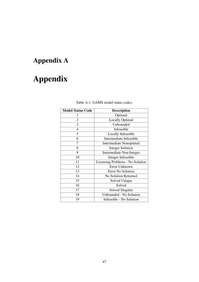
Appendix A

Appendix

Table A.1: GAMS model status codes.

Model Status Code Description1 Optimal2 Locally Optimal3 Unbounded4 Infeasible5 Locally Infeasible6 Intermediate Infeasible7 Intermediate Nonoptimal8 Integer Solution9 Intermediate Non-Integer

10 Integer Infeasible11 Licensing Problems - No Solution12 Error Unknown13 Error No Solution14 No Solution Returned15 Solved Unique16 Solved17 Solved Singular18 Unbounded - No Solution19 Infeasible - No Solution

47

48 Appendix

Table A.2: Cumulative results of one-week simulation under Big-M method-Plugged probability

ε









Expected costs(e) 233,13 829,35 205,99 959,41 120,49 1125,80 71,81 1175,17 28,24 1254,78


Table A.3: Cumulative results of one-week simulation under Big-M method-Available probability

ε









Expected costs(e) 206,05 733,82 182,80 842,35 90,79 914,93 64,30 1009,70 56,49 1225,48


References

[1] EEA. Total greenhouse gas emissions from transport. Indicator Assessment - Data andmaps, page 13, 2018. URL: https://www.eea.europa.eu/data-and-maps/indicators/transport-emissions-of-greenhouse-gases/transport-emissions-of-greenhouse-gases-11.

[2] White paper. URL: https://eur-lex.europa.eu/legal-content/EN/TXT/PDF/?uri=CELEX:52011DC0144&from=EN.

[3] Tiago Soares, Tiago Sousa, Peter Bach Andersen, and Pierre Pinson. Optimal offeringstrategy of an EV aggregator in the frequency-controlled normal operation reserve mar-ket. International Conference on the European Energy Market, EEM, 2018-June:1–6, 2018.doi:10.1109/EEM.2018.8469922.

[4] Adrene Briones, James Francfort, Paul Heitmann, Michael Schey, Steven Schey, and J Smart.Vehicle-to-grid (v2g) power flow regulations and building codes review by the avta. IdahoNational Lab., Idaho Falls, ID, USA, 2012.

[5] K Fell, K Huber, B Zink, R Kalisch, D Forfia, D Hazelwood, N Dang, D Gionet, M Musto,W Johnson, et al. Assessment of plug-in electric vehicle integration with iso/rto systems.KEMA, Inc. and ISO/RTO Council, 2010.

[6] Stylianos I. Vagropoulos and Anastasios G. Bakirtzis. Optimal bidding strategy for elec-tric vehicle aggregators in electricity markets. IEEE Transactions on Power Systems,28(4):4031–4041, 2013. doi:10.1109/TPWRS.2013.2274673.

[7] Alec N Brooks. Final Report Grid Regulation Ancillary Service. Regulation,(01):61, 2002. URL: http://www.smartgridnews.com/artman/uploads/1/sgnr_2007_12031.pdf.

[8] Ivan Pavic, Tomislav Capuder, and Hrvoje Pandzic. Profit margin of electric vehicle batteryaggregator. 2018 IEEE International Energy Conference, ENERGYCON 2018, pages 1–6,2018. doi:10.1109/ENERGYCON.2018.8398790.

[9] A New Model. A New Model. 2008.

[10] Willett Kempton and Jasna Tomic. Vehicle-to-grid power fundamentals: Calculating capacityand net revenue. Journal of Power Sources, 144(1):268–279, 2005. arXiv:arXiv:0909.0931v2, doi:10.1016/j.jpowsour.2004.12.025.

[11] Ricardo J. Bessa, Manuel A. Matos, Filipe Joel Soares, and João A.Peças Lopes. Optimizedbidding of a EV aggregation agent in the electricity market. IEEE Transactions on SmartGrid, 3(1):443–452, 2012. doi:10.1109/TSG.2011.2159632.

49

https://www.eea.europa.eu/data-and-maps/indicators/transport-emissions-of-greenhouse-gases/transport-emissions-of-greenhouse-gases-11



https://eur-lex.europa.eu/legal-content/EN/TXT/PDF/?uri=CELEX:52011DC0144&from=EN

https://eur-lex.europa.eu/legal-content/EN/TXT/PDF/?uri=CELEX:52011DC0144&from=EN

http://dx.doi.org/10.1109/EEM.2018.8469922

http://dx.doi.org/10.1109/TPWRS.2013.2274673

http://www.smartgridnews.com/artman/uploads/1/sgnr_2007_12031.pdf

http://www.smartgridnews.com/artman/uploads/1/sgnr_2007_12031.pdf

http://dx.doi.org/10.1109/ENERGYCON.2018.8398790

http://arxiv.org/abs/arXiv:0909.0931v2

http://arxiv.org/abs/arXiv:0909.0931v2

http://dx.doi.org/10.1016/j.jpowsour.2004.12.025

http://dx.doi.org/10.1109/TSG.2011.2159632

50 REFERENCES

[12] D Rua, Student Member, D Issicaba, F J Soares, Student Member, P M Rocha Almeida,Student Member, R J Rei, J A Peças Lopes, and Senior Member. Advanced Meter-ing Infrastructure Functionalities for Electric Mobility. 241399(241399), 2008. doi:10.1109/ISGTEUROPE.2010.5638854.

[13] Lav Agarwal and Wang Peng. Using EV Battery Packs for Vehicle-to-Grid Applications :An Economic Analysis. 2014 IEEE Innovative Smart Grid Technologies - Asia (ISGT ASIA),pages 663–668, 2020. doi:10.1109/ISGT-Asia.2014.6873871.

[14] Tugrul U. Daim, Xiaowen Wang, Kelly Cowan, and Tom Shott. Technology roadmapfor smart electric vehicle-to-grid (V2G) of residential chargers. Journal of Inno-vation and Entrepreneurship, 5(1), 2016. URL: http://dx.doi.org/10.1186/s13731-016-0043-y, doi:10.1186/s13731-016-0043-y.

[15] João Paulo Tomé Saraiva, Maria Teresa Costa Pereira da Silva, and Ponce de Leão. Mercadosde Electricidade-Regulação e Tarifação de Uso das Redes. FEUP edições, 2002.

[16] Transmission system operator. URL: http://www.entsoe-event.eu/transmission_system_operator.html.

[17] Willett Kempton. ELECTRIC VEHICLES AS A NEW POWER ELECTRIC UTILITIESSOURCE FOR. 2(3):157–175, 1997.

[18] Yann G. Rebours, Daniel S. Kirschen, Marc Trotignon, and Sebastien Rossignol. A Survey ofFrequency and Voltage Control Ancillary Services - Part I: Technical Features. IEEE Trans-actions on Power Systems, 22(1):350–357, 2007. doi:10.1109/TPWRS.2006.888963.

[19] Balancing and ancillary services markets. URL: https://www.entsoe.eu/about/market/#balancing-and-ancillary-services-markets.

[20] UCTE. P1: Load-Frequency Control and Performance. Continental Europe Op-eration Handbook, (Cc):P1–1–P1–32, 2009. URL: https://www.entsoe.eu/fileadmin/user_upload/_library/publications/entsoe/Operation_Handbook/Policy_1_final.pdf.

[21] REN. Manual de procedimentos do gestor do sistema. 2008.

[22] ENERGINET. ANCILLARY SERVICES TO BE DELIVERED IN DEN-MARK TENDER CONDITIONS . https://en.energinet.dk/-/media/B225651649124625B6F83BA70BA0EC0B.pdf. [Online].

[23] H. Sekyung, H. Soohee, and K. Sezaki. Development of an Optimal Vehicle-to-GridAggregator for Frequency Regulation. IEEE Transactions on Smart Grid, 1(1):65–72, 2010. URL: http://ieeexplore.ieee.org/document/5446440/, doi:10.1109/TSG.2010.2045163.

[24] Trine Krogh Kristoffersen, Karsten Capion, and Peter Meibom. Optimal charging ofelectric drive vehicles in a market environment. Applied Energy, 88(5):1940–1948,2011. URL: http://dx.doi.org/10.1016/j.apenergy.2010.12.015, doi:10.1016/j.apenergy.2010.12.015.

[25] Muhammad Ansari, Ali T. Al-Awami, Eric Sortomme, and M. A. Abido. Coordinated bid-ding of ancillary services for vehicle-to-grid using fuzzy optimization. IEEE Transactionson Smart Grid, 6(1):261–270, 2015. doi:10.1109/TSG.2014.2341625.

http://dx.doi.org/10.1109/ISGTEUROPE.2010.5638854

http://dx.doi.org/10.1109/ISGTEUROPE.2010.5638854

http://dx.doi.org/10.1109/ISGT-Asia.2014.6873871

http://dx.doi.org/10.1186/s13731-016-0043-y

http://dx.doi.org/10.1186/s13731-016-0043-y

http://dx.doi.org/10.1186/s13731-016-0043-y

http://www.entsoe-event.eu/transmission_system_operator.html

http://www.entsoe-event.eu/transmission_system_operator.html


https://www.entsoe.eu/about/market/#balancing-and-ancillary-services-markets

https://www.entsoe.eu/about/market/#balancing-and-ancillary-services-markets

https://www.entsoe.eu/fileadmin/user_upload/_library/publications/entsoe/Operation_Handbook/Policy_1_final.pdf



https://en.energinet.dk/-/media/B225651649124625B6F83BA70BA0EC0B.pdf

https://en.energinet.dk/-/media/B225651649124625B6F83BA70BA0EC0B.pdf

http://ieeexplore.ieee.org/document/5446440/



http://dx.doi.org/10.1016/j.apenergy.2010.12.015




REFERENCES 51

[26] M. Rahmani-Andebili. Plug-in Electric Vehicles (PIEVs) aggregator as a renewable source indistribution network. 2012 Proceedings of 17th Conference on Electrical Power Distribution,EPDC 2012, pages 1–4, 2012.

[27] Stylianos I. Vagropoulos and Anastasios G. Bakirtzis. Optimal bidding strategy for elec-tric vehicle aggregators in electricity markets. IEEE Transactions on Power Systems,28(4):4031–4041, 2013. doi:10.1109/TPWRS.2013.2274673.

[28] Mushfiqur R. Sarker, Yury Dvorkin, and Miguel A. Ortega-Vazquez. Optimal participation ofan electric vehicle aggregator in day-ahead energy and reserve markets. IEEE Transactionson Power Systems, 31(5):3506–3515, 2016. doi:10.1109/TPWRS.2015.2496551.

[29] Christoph Goebel and Hans Arno Jacobsen. Aggregator-Controlled EV Charging in Pay-as-Bid Reserve Markets with Strict Delivery Constraints. IEEE Transactions on Power Systems,31(6):4447–4461, 2016. doi:10.1109/TPWRS.2016.2518648.

[30] Ricardo J. Bessa and Manuel A. Matos. Optimization models for EV aggregator participationin a manual reserve market. IEEE Transactions on Power Systems, 28(3):3085–3095, 2013.doi:10.1109/TPWRS.2012.2233222.

[31] Behzad Vatandoust, Ali Ahmadian, Masoud Golka, Ali Elkamel, Ali Almansoori, and Mo-hammad Ghaljehei. Risk-Averse Optimal Bidding of Electric Vehicles and Energy StorageAggregator in Day-ahead Frequency Regulation Market. IEEE Transactions on Power Sys-tems, 8950(c), 2018. doi:10.1109/TPWRS.2018.2888942.

[32] Eric Sortomme and Mohamed A. El-Sharkawi. Optimal combined bidding of vehicle-to-gridancillary services. IEEE Transactions on Smart Grid, 3(1):70–79, 2012. doi:10.1109/TSG.2011.2170099.

[33] John F. Franco, Marcos J. Rider, and Ruben Romero. A Mixed-Integer Linear ProgrammingModel for the Electric Vehicle Charging Coordination Problem in Unbalanced ElectricalDistribution Systems. IEEE Transactions on Smart Grid, 6(5):2200–2210, 2015. doi:10.1109/TSG.2015.2394489.

[34] K. Clement, E. Haesen, and J. Driesen. Stochastic analysis of the impact of plug-in hybridelectric vehicles on the distribution grid. 25(1):160–160, 2009. doi:10.1049/cp.2009.0590.

[35] Jonas Fluhr, Klaus Henning Ahlert, and Christof Weinhardt. A stochastic model for sim-ulating the availability of electric vehicles for services to the power grid. Proceedingsof the Annual Hawaii International Conference on System Sciences, pages 1–10, 2010.doi:10.1109/HICSS.2010.33.

[36] Amir H Hajimiragha, Claudio A Cañizares, Michael W Fowler, Somayeh Moazeni, AliElkamel, and B Indices. A Robust Optimization Approach for Planning the Transition toPlug-in Hybrid Electric Vehicles. 26(4):2264–2274, 2011. doi:10.1109/TPWRS.2011.2108322.

[37] Wencong Su and Mo Yuen Chow. Evaluation on intelligent energy management system forPHEVs/PEVs using Monte Carlo method. DRPT 2011 - 2011 4th International Conferenceon Electric Utility Deregulation and Restructuring and Power Technologies, pages 1675–1680, 2011. doi:10.1109/DRPT.2011.5994167.










http://dx.doi.org/10.1049/cp.2009.0590

http://dx.doi.org/10.1049/cp.2009.0590

http://dx.doi.org/10.1109/HICSS.2010.33



http://dx.doi.org/10.1109/DRPT.2011.5994167

52 REFERENCES

[38] Olle Sundstr. Optimization Methods to Plan the Charging of Electric Vehicle Fleets.

[39] J Soares, T Sousa, H Morais, Z Vale, B Canizes, and A Silva. Application-Specific Modi-fied Particle Swarm Optimization for energy resource scheduling considering vehicle-to-grid.Applied Soft Computing Journal, 13(11):4264–4280, 2013. URL: http://dx.doi.org/10.1016/j.asoc.2013.07.003, doi:10.1016/j.asoc.2013.07.003.

[40] Jian Zhao, Can Wan, Zhao Xu, and Jianhui Wang. Risk-Based Day-Ahead Scheduling ofElectric Vehicle Aggregator Using Information Gap Decision Theory. IEEE Transactions onSmart Grid, 8(4):1609–1618, 2017. doi:10.1109/TSG.2015.2494371.

[41] Olle Sundström and Carl Binding. Flexible charging optimization for electric vehicles con-sidering distribution grid constraints. IEEE Transactions on Smart Grid, 3(1):26–37, 2012.doi:10.1109/TSG.2011.2168431.

[42] Ricardo Bessa. Methodologies for the participation of an electric vehicles’ aggregator in theelectricity market. (April):309, 2013.

[43] Niklas Rotering and Marija Ilic. Optimal charge control of plug-in hybrid electric vehiclesin deregulated electricity markets. IEEE Transactions on Power Systems, 26(3):1021–1029,2011. doi:10.1109/TPWRS.2010.2086083.

[44] Riadh Henrion Ren Mller Andris van, Wim Zorgati. Chance constrained programming andits applications to energy management. Weierstrass Institute Berlin, 2012.

[45] Bo Zeng, Yu An, and Ludwig Kuznia. Chance Constrained Mixed Integer Program: Bilinearand Linear Formulations, and Benders Decomposition. (1), 2014. URL: http://arxiv.org/abs/1403.7875, arXiv:1403.7875, doi:10.1038/nclimate2483.

[46] Pedro M Castro. A Tighter Piecewise McCormick Relaxation for Bilinear Problems Prob-lem definition (NLP). 2014. URL: http://minlp.cheme.cmu.edu/2014/papers/castro.pdf.

[47] Parker project [online]. URL: https://parker-project.com/.

[48] Energinet. URL: https://energinet.dk/.

[49] MATLAB. Introduction - product overview. The MathWorks, 2010.

[50] R. E. Rosenthal. Gams – a user’s guide. GAMS Development Corporation, 2008.

http://dx.doi.org/10.1016/j.asoc.2013.07.003






http://arxiv.org/abs/1403.7875



http://dx.doi.org/10.1038/nclimate2483

http://minlp.cheme.cmu.edu/2014/papers/castro.pdf

http://minlp.cheme.cmu.edu/2014/papers/castro.pdf

https://parker-project.com/

https://energinet.dk/

a chance-constrained approach for electric vehicle ... · electric vehicle aggregator participation...

Documents