WP/09/73

A Coincident Indicator of the

Gulf Cooperation Council (GCC) Business Cycle

Abdullah Al-Hassan

© 2009 International Monetary Fund WP/09/73 IMF Working Paper Monetary and Capital Markets Department

A Coincident Indicator of the Gulf Cooperation Council (GCC) Business Cycle

Prepared by Abdullah Al-Hassan

Authorized for distribution by Daniel Hardy

April 2009

Abstract

This Working Paper should not be reported as representing the views of the IMF. The views expressed in this Working Paper are those of the author(s) and do not necessarily represent those of the IMF or IMF policy. Working Papers describe research in progress by the author(s) and are published to elicit comments and to further debate.

This paper constructs a coincident indicator for the Gulf Cooperation Council (GCC) area business cycle. The resulting coincident indicator provides a reliable measure of the GCC business cycle; over the last decade, the GCC coincident index and the real GDP growth have moved closely together. Since the indicator is constructed using a small number of common factors, the strong correlation between the indicator and real GDP growth points to a high degree of commonality across GCC economies. The timing and direction of movements in macroeconomic variables are characterized with respect to the coincident indicator. Finally, to obtain a meaningful economic interpretation of the latent factors, their behavior is compared to the observed economic variables. JEL Classification Numbers: E60, E61 Keywords: GCC monetary union, factor models, GDFM, and business cycle indicators. Author’s E-Mail Address: aalhassan@imf.org

2

Contents Page

I. Introduction ............................................................................................................................3

II. Methodology .........................................................................................................................6 A. Generalized Dynamic Factor Model .........................................................................6 B. Estimating Common Components by a One-Sided Filter .........................................8

III. Building a GCC Area Database .........................................................................................13

IV. A Coincident Indicator for the GCC Business Cycle ........................................................15 A. Definition of the Coincident Indicator Properties...................................................15 B. Properties of the Coincident Indicator ....................................................................18 C. The Construction of a Coincident Indicator............................................................19

V. Degree of Commonality and Cyclical Behavior of the Variables ......................................23 A. Degree of Commonality..........................................................................................23 B. Business Cycle: Stylized Facts................................................................................24

VI. Observed Economic Variables and Latent Factors............................................................27

VII. Conclusion........................................................................................................................29

References................................................................................................................................33 Tables 1. The Direction and Timing of Variables Against the Coincident Indicator..........................24 2. Testing the Observed Macroeconomic Data Against the Latent Factors ............................29 Figures 1. Average Dynamic Eigenvalues Over Cross-Sectional Units...............................................11 2. Percentage of Variance Explained .......................................................................................12 3. Spectral Density Functions of All Eigenvalues ...................................................................17 4. Average of Spectral Density Functions ...............................................................................17 5. The GCC Coincident Indicator and the GCC Area GDP Growth Rate...............................20 6. The GCC Coincident Indicator and the Common Component of National GDP................21 7. The GCC Coincident Indicator and the Common Component of National GDP................22 Appendix I: Data Set ................................................................................................................................31 Appendix Tables 1: Data, Degree of Commonality, and Cyclical Behavior .......................................................31

3

I. INTRODUCTION

The Gulf Cooperation Council (GCC) plans to launch a single currency by 2010 in its six member countries: Bahrain, Kuwait, Oman, Qatar, Saudi Arabia, and the United Arab Emirates.1 With the creation of the GCC Monetary Union, a single and indivisible common monetary policy will be based on GCC-wide economic and financial developments. Therefore, prospective policymakers at the GCC supernational monetary agency will need to scrutinize a large number of economic variables, both at the national and regional level, in order to obtain a clear signal about the current and future state of the GCC economies. Having an economic indicator that synthesis information coming from different sources may assist monetary policymakers in conducting a sound monetary policy. In order to assess the business cycle evolution for the GCC area, policymakers will examine any economic variables that may provide them with timely information about the likely economic developments of that region. Since economic data are controlled by different agencies, not all economic variables are released simultaneously, and with various lags and frequencies. Hence, policymakers will have to make decisions with the partial information available to them yet.

To overcome this problem, I constructed a timely single coincident index that can closely track the business cycle evolution of the GCC area. This indicator may provide policymakers and the business community with a timely and clear signal of the underlying direction of the GCC economies. Finally, the indicator can be constructed at relatively high frequency and with partial information.

The first business cycle indicator was constructed in 1920 by the National Bureau of Economic Research (NBER) to describe the business cycle expansions and contractions for the U.S. economy. The seminal work of Burns and Mitchell (1946) describes the business cycle as a type of fluctuation in many time series across different sectors of the economy at the same time: “A cycle consists of expansions occurring at about the same time in many economic activities, followed by similarly general recessions, contractions, and revivals which merge into the expansion phase of the next cycle; this sequence of changes is recurrent but not periodic; in duration business cycles vary from more than one year to ten or twelve years; they are not divisible into shorter cycles of similar character with amplitudes approximating their own.”

1 In November 2006, Oman indicated that it may not be able to join the monetary union by 2010 because it cannot meet some of the convergence criteria due to its massive infrastructure projects. Furthermore, on May 2007, Kuwait de-pegged its currency to the U.S. dollar. Therefore, these actions may jeopardize the introduction of the single currency by 2010.

4

Burns and Mitchell (1946) were the first to empirically describe the procedures employed by the NBER to construct a U.S. business cycle indicator. The indicator is constructed by averaging the contemporaneous time series into one single index. In the NBER method, researchers have to determine the peaks and troughs of a “good” reference series and then classify other series as lagging, leading, or coincident variables by how “close” they are to the reference series. Although the NBER methodology is not based on a well-defined statistical model, it still produces an accurate measure of U.S. activity by identifying the troughs and peaks dates that frame U.S. recessions and expansions.

As computing power has increased over the last three decades, econometricians have consequently developed more statistically oriented models. One set of these models is the factor model in which a large panel of data is driven by few common shocks.2 In order to construct a real-time coincident indicator for the GCC area business cycle, this paper utilizes an innovative approach to factor models. Specifically, it implements the Generalized Dynamic Factor Model (GDFM) proposed by Forni et al. (2000, 2004, and 2005).

The constructed indicator may be a good analytical and empirical tool for policymakers at the prospective GCC supernational monetary agency since it provides them with a clear signal about the current economic state by synthesizing a large amount of information obtained from different sources. This indicator has three distinct properties: first, it effectively exploits the covariance structure across many economic variables within and among the GCC economies; second, it is purged of high frequency volatility and seasonal components which are irrelevant to business cycle analyses; and finally, it is free from both measurement errors and national idiosyncratic shocks.

To achieve the previous desirable properties, Altissimo et al. (2001) identify four problems that need to be addressed before constructing any coincident or leading indicator: (i) data are not available on a comparable basis for a long period of time; (ii) data are released in a non-synchronous way; (iii) GDP data is usually not available on a short horizon basis; and (iv) data must be appropriately filtered so that the cyclical component of the GDP growth is continually adjusted as new data become available. Therefore, the first task of this paper is to construct a GCC area databank covering a wide range of economic variables, which may help in explaining the GCC business cycle fluctuations. To that end, macroeconomic variables are collected from different sources to construct a dataset that covers a wide range of economic phenomena for the GCC economies, because there is not yet a single dataset containing macroeconomic time series for the GCC area. The second task of this paper is to construct a real time coincident index of the GCC business cycle. This index is similar to the EuroCoin index proposed by Altissimo et al. (2001) and published monthly by the Centre for Economic Policy Research (CEPR). 2 Factor models are merely a formal representation of the index model used by Burns and Mitchell (1946), in which the common factors take on the role of the single index.

5

The GDFM is a novel development in the theory of factor models. Similar to any factor model, it summarizes the information available in a large cross-section of time series by a few common shocks. That is, the movement of any time series can be represented as the sum of two mutually orthogonal unobservable components: a common component and an idiosyncratic component. The common component is a linear combination of common shocks, and thereby, it is strongly correlated with the rest of the panel. By contrast, the idiosyncratic component is a variable-specific shock and it is weakly correlated across the panel. Since those two components are unobservable, they have to be estimated. The common shocks are estimated by means of dynamic principal components. Unlike the static principal components method, which is based on the eigenvalues decomposition of the contemporaneous covariance matrix, the dynamic principal components method relies on the spectral density matrix of the data wherein data are weighted and shifted across time (dynamic co-variations). In addition, the real-time coincident indicator (a reference cycle) is defined as the cyclical common component of real GDP growth of the GCC area after filtering out measurement errors and idiosyncratic noises, as well as seasonal components. By utilizing GDFM, the business cycle information contained in each variable can be measured as the variance of its cyclical common component relative to its total variance. Further, by using the dynamic principal components instead of static principal components, GDFM allows each variable in the dataset to be classified as pro-cyclical or counter-cyclical with respect to the reference cycle. The GDFM then categorizes the direction of each variable against the reference cycle as lagging, coincident, or leading. All of these results can provide policymakers at the GCC supernational monetary agency with some useful tools to assess the current economic situation in the GCC area and its likely future developments. The results conveyed in this paper are distinguishable from the existing literature in the following ways: first, to my knowledge, this is an original effort to generate a real-time coincident indicator for the GCC region by utilizing GDFM; second, while most of the previous literature had been applied to the Euro area, the Asian Pacific area, or to the United States, this paper constructs a business cycle indicator for the GCC area that has been increasingly important in the global economy because of its abundant financial and natural resources. Since the GCC region has a unique economic structure due to a large share of hydrocarbon sector, the movement in oil prices may play a vital role in explaining the fluctuations of the business cycle in the GCC area.

Finally, while there are some well-established and large databases for the U.S. and Euro areas, there is no single dataset containing macroeconomic time series for the GCC area. The construction of the databank and the real-time coincident indicator in this paper can facilitate future research on the GCC economies.

The remainder of this paper is organized as follows: Section 2 gives an overview of the Generalized Dynamic Factor Model; Section 3 describes the procedures of constructing the GCC dataset; Section 4 defines the desired properties and estimation procedures of the

6

coincident indicator of the GCC business cycle; Section 5 defines the degree of commonality and cyclical behavior of all individual time series in the dataset; Section 6 examines the proximity of the individual observed economic variables to the latent factors; and Section 7 concludes.

II. METHODOLOGY

This section gives an overview of the Generalized Dynamic Factor Model (GDFM) that is proposed by Forni et al. (2000, 2004, and 2005). Forni and Lippi (2001) illustrate the representation theory of GDFM. Theoretically, GDFM encompasses an approximate factor model of Chamberlain and Rothschild (1983) and Chamberlain (1983), in that idiosyncratic components are allowed to be weakly correlated across the panel, but the factors are static. It also generalizes the factor models of Sargent and Sim (1977) and Geweke (1977), in which the factors are dynamic, but there is no cross-correlation among idiosyncratic components at any lead and lag.

A. Generalized Dynamic Factor Model

The i-th time series, after suitable transformations, is a realization of real-value process from a zero-mean, wide-sense stationary process ity . All y are co-stationary, where stationarity holds for the n-dimensional vector process 1 2( , ,..., )t t nty y y ′ for any n. Formally, any given time series can be represented as the sum of two mutually orthogonal unobservable components: the common component, itχ , and the idiosyncratic component, itξ :

( )it it it i t ity b Lχ ξ ξ= + = +u (1)

where ity is a stationary process for the i-th time series, i= 1,…, n, at time t, t = 1,…, T. The common component, itχ , is driven by q common factors (or common shocks)

1 2( , ,..., )t t t qtu u u ′=u , for example, a technology shock, a demand shock, an oil shock. In any factor models, the number of common shocks q is much less than the number of variables n; q n<< .3 These common shocks are loaded with different coefficients and finite (or infinite) number of lags; that is, variables in the panel are allowed to react heterogeneously to shocks. Thus, the common component can be re-written as a dynamic linear combination of the q common shocks:

1

( )q

it ij jtj

b L uχ=

=∑ (2)

The common component captures the part of the time series which commoves with the rest of macroeconomic variables. By contrast, the idiosyncratic component, itξ , is driven

3 Sargent and Sims (1977), and Giannone et al. (2002, and 2004) present some evidence using different datasets that few shocks are capable of explaining the dynamics of macroeconomic data.

7

exclusively by a variable-specific shocks such as measurement errors or variable specific disturbances. The distinction between the common component and the idiosyncratic component has an important implication for policymakers as to how to react to a specific shock. By identifying the source of a shock, they can decide whether to carry out local and sectoral measures, or common measures. We rewrite the previous equations in a matrix notation:

= + ( )t t t n t tB L= +y χ ξ u ξ (3)

Equation (3) is a GDFM4, where 1 2( , ,..., )t t t nty y y ′=y , ,n t∈ , is a stationary process vector with zero mean and finite second order moments E[ ],k t t k k−′= ∈Γ y y , 1 2( , ,..., )t t t ntχ χ χ ′=χ is the common component vector, and 1 2( , ,..., )t t t ntξ ξ ξ ′=ξ is the idiosyncratic component vector in which its entries are orthogonal to , for any , , and j t ku j t k− .

0 1( ) ... ssL B B L B L= + + +B is ( x )n q polynomial matrix of order s in the lag operator L,

whose coefficients represent the impulse response function of ity to any specific shock jtu . Unlike the static factor model, GDFM is dynamic in a sense that the common shocks are allowed to hit the series at different times. Finally, tu is an orthonormal q dimensional white noise vector, that is, jtu has a unit variance and is orthogonal to stu for any s j≠ . Forni et al. (2000) impose two additional assumptions to specify the model by separating the idiosyncratic sources of variation from the common sources of variation. The first assumption allows for a limited serial and cross-sectional correlation among idiosyncratic components, which tends to zero as i → ∞ . That is, even though the idiosyncratic sources of variations can be shared by many series, the assumption of boundness guarantees that their effect is limited to a finite number of series. The second assumption ensures a minimum amount of cross-correlation among common components, that is,. the common shocks are present in infinite cross-sectional series.

The moving average representation of GDFM in equation (3) can be easily written in a static form by loading the common factors only contemporaneously. Defining an x 1r vector as:

, , ...,-1 -( ) ( )t t t t t sN L ′= = u u uf u where ( )N L is an x r q absolutely summable matrix function of L. The common component in (3) can be written as:

t n tA=χ f (4)

where 1 2 0 1( , ,..., ) ( , ,..., )n n nn n sA a a a B B B′ ′ ′ ′= = is x n r matrix, and ( 1)r q s= + is the number of

static factors in tf . Note that r entries of tf denote the static factors, whereas the q entries of

4 References to n will not be made explicit in ty , tχ , tξ , and kΓ to avoid heavy notations. Similarly, explicit

reference for T in kΓ will be omitted.

8

tu denote the dynamic factors. To be precise, 1 1 1and t tu u − are two different static factors of the same common shock. Therefore, the common component is only driven by the q exogenous shocks (dynamic factors) and it can be expressed at the same time as a linear combination of r static factors. In the GDFM model, q represents the rank of the spectral density matrix of χ , which is determined by the common sources of exogenous variations to all variables. On the other hand, r is the rank of the contemporaneous covariance matrix of χ , which is determined by the degree of heterogeneity of the impulse response functions to the q exogenous shocks. The distinction between static and dynamic factors has an important implication for policymakers. While knowing the number of the dynamic factors can provide them with the necessary information in understanding the main sources of business cycle fluctuations, the static factors explain how each economic variable react to the dynamic factors.

B. Estimating Common Components by a One-Sided Filter

It is not feasible to obtain a consistent estimate and forecast of the common component from equation (3) since the common component estimator is a two-sided filter of ty (see Forni et al. 2000)5. That is, the forecasting performance deteriorates as t approaches T or 1, which is an unpleasant characteristic for forecasting. To overcome the previous caveat, Forni et al. (2005) propose a two-step method to estimate and forecast the common components using a one-sided filter. In the first step, an estimate of the spectral density matrix ( )θΣ of the observable ty is obtained. Then, the estimated spectral density matrix can be correspondingly decomposed into spectral density matrices of the common and the idiosyncratic components through the dynamic principal component method. To close the first step, the Inverse Fourier Transform is applied to the estimated spectral density matrices in order to obtain the covariance matrices of the common and idiosyncratic components at all leads and lags, respectively. The second step consists of estimating the static factors by utilizing the generalized principal component approach. Finally, in-sample estimation and forecasting of the common components can be derived by the orthogonal projection of the common components onto the space spanned by the estimated static factors.

Step 1: Estimating the Covariance Structure of the Common and Idiosyncratic Component The estimated spectral density matrix, ( )θΣ , can be obtained by applying a discrete Fourier Transform to the estimated covariance matrices kΓ of ty . The spectral representation theorem allows us to represent the covariance matrices as a sum (integral) of elementary

5 Since the projection coefficients of common components, ( )ijb L , are obtained by the inverse Fourier transform of the first q dynamic eigenvectors, those coefficients are two-sided.

9

orthogonal periodic processes, which is fruitful for the dynamic analysis. More precisely, for some selected integer ( )M M T= 6, the sample covariance matrices E[ ]k t t k−′=Γ y y of ty are

computed with ,....,k M M= − and k k− ′=Γ Γ . The estimated spectral density matrix, ( )θΣ , is then obtained by multiplying the sample covariance matrices by a Bartlett lag-window7, 1

1k

kM

ω = −+

, and applying the discrete Fourier Transform:

1( ) 2

Mi k

h k kk M

e θθ ωπ

−

=−

= ⋅ ⋅∑Σ Γ (5)

The spectra are evaluated at (2 1)M + equally spaced frequencies in the interval [ , ]π π− ; i.e. 2

(2 1)hh

Mπθ =+

with ,....,h M M= − .

The estimated spectral density matrix of the data ( )θΣ can be decomposed into two orthogonal components as:

{ {rank rank rank

( ) ( ) ( )n nq

χ ξθ θ θ= +Σ Σ Σ123 (6)

The decomposition in (6) is obtained by applying the dynamic principal component analysis (Brillinger, 1981, paper 9)8. That is, for each frequency of the grid, the eigenvalues and corresponding eigenvectors of ( )hθΣ are computed. Then, by ordering the eigenvalues in descending order and collecting the corresponding eigenvectors for each frequency, we obtain the j-th dynamic eigenvalue functions ( )jλ θ of ( )θΣ and the corresponding dynamic

eigenvectors functions 1( ) ( ( ).... ( ))j j jnp pθ θ θ=p , for 1,....,j n= . For each frequency, denote

( )q θΛ to be a q x q diagonal matrix, diag 1( ( ),...., ( ))qλ θ λ θ , of the spectral eigenvalues, and

the corresponding x n q eigenvectors by 1( ) ( ( ),...., ( ))q qθ θ θ=P p p . Following Forni et al.

(2000), the estimated spectral density matrix of the common component 1( ,...., )t t ntχ χ ′=χ is given by:

( ) ( ) ( ) ( )q q qχ θ θ θ θ ′=Σ P Λ P (7)

It follows immediately from (7) that the estimated spectral density matrix of the idiosyncratic components is then computed as the difference:

6 Forni et al. (2000) show that a fixed rule ( ) ( )M M T round T= = performs well in simulations.

7 Bartlett weights are needed to avoid biases caused by truncating the population spectral density.

8 Static principal component analysis does not take into account the autocovariances, but just the covariances. Therefore, it does not maximize the variance explained. Also, Brillinger (1981) shows that the first q principal components are the best linear combinations of the data.

10

( ) ( ) ( )ξ χθ θ θ= −Σ Σ Σ (8)

Finally, applying the Inverse Discrete Fourier Transform to (7) and (8) gives the estimated covariance matrices of the common components at different leads and lags:

2( ) ( )2 1

2( ) ( )2 1

h

h

Mi k

k hh M

Mi k

k hh M

eM

eM

θχ χ

θξ ξ

π θ

π θ

=−

=−

= ⋅+

= ⋅+

∑

∑

Γ Σ

Γ Σ (9)

Until now, we have not imposed any criteria on how to choose the optimal number of common shocks, q. Forni et al. (2000) propose a decision rule to determine q. To choose the optimal number of q, the eigenvalues of the dataset’s spectral density matrix,

( ) for 1,....,k h k nθ =Σ , have to satisfy the following two conditions: 1. The average over the frequencies θ of the first q eigenvalues diverges, whereas the

average of the th( 1)q + eigenvalues is relatively stable. 2. When k n= , there is a substantial difference between the explained variance of the

first thq principal components, and the variance explained by the th( 1)q + principal components.

With regard to the first criteria, Figure 1 shows the first 20 dynamic eigenvalues averaged over low frequencies; that is, business cycle frequencies defined to be more than five quarters. It is plotted against the number of the cross-sectional units n. The figure clearly shows that only the first three dynamic eigenvalues diverge most probably, whereas the remaining eigenvalues are bounded.

11

Figure 1. Average Dynamic Eigenvalues Over Cross-Sectional Units

20 30 40 50 60 70 80

1

2

3

4

5

6

7

8

9

10

Num ber o f c ross-sec tion units

varia

nce/

2pi

The second criteria suggests to add a factor at a time until the additional variance explained by the last dynamic principal component is at least larger than a pre-specified critical value, that is, 5 or 10 percent of the total variance. As in Altissimo et al. (2001) and Forni et al. (2000), I set the marginal explained variance at 10 percent. Figure 2 shows the percentage of variance explained by the first 10 dynamic principal components. Each of the first three dynamic principal components explains more than 10 percent. As it can be seen, the first three dynamic principal components together explain on average 50 percent of the total variance of the 82 series. Therefore, the number of the common shocks that is chosen throughout the remainder of this paper is in accordance with the previous empirical literatures. For instance, Forni and Reichlin (1998) and Forni et al. (2000) find 2q = , Reijer (2005) and Schneider and Spitzer (2004) find 3q = , and Altissimo et al. (2001) find 4q = .

12

Figure 2. Percentage of Variance Explained

0%

5%

10%

15%

20%

25%

1 2 3 4 5 6 7 8 9 10

Num ber of Dynam ic P rinc ipal Com ponents

Exp

lain

ed v

aria

nce

The estimates of the covariance matrices of the cyclical components, 1 2( , ,..., )C C C C

t t t ntχ χ χ ′=χ ,9 can be obtained by applying the Inverse Discrete Fourier Transform to the frequency band of interest [ 2 / , 2 / ]π τ π τ− :

2( ) ( )

2 1C

h

Hi k

k hh H

eH

θχ χπ θ=−

= ⋅+ ∑Γ Σ (10)

where H is defined by the condition /(2 1)H M τ+ > and ( 1) /(2 1)H M τ+ + < . Thus, to eliminate waves of periodicity shorter than 5 quarters, I set 5τ = . Step 2: Estimating and Forecasting the Common Components Forni et al. (2005) estimate the r contemporaneous linear combination of ty as the solution of the generalized principal component problem. The information criteria proposed by Bai and Ng (2002) will be used to determine r. More precisely, starting from the estimated covariance matrices, (10), Forni et al. (2005) compute the generalized eigenvalues jμ ; that is, n

complex number solving det 0 0( )χ ζμ−Γ Γ , and the corresponding eigenvectors jZ for 1,....,j n= . The vectors are the solution of:

9 With any stationary variable, the common component of variable i can be decomposed into the sum of waves of different periodicity, i.e. C NC

it it itχ χ χ= + , where Citχ is represented by smooth waves with long and medium-

run periodicity, while NCitχ is represented by high-frequency volatility.

13

0 0j j jχ ζμ=Z Γ Z Γ (11)

and the normalizing condition:

0

0 for 1 for j i

j ij i

ζ ≠′ =

=Z Γ Z (12)

By ordering the eigenvalues in descending order and taking the corresponding eigenvectors of the r largest eigenvalues, the estimated static factors are the generalized principal components:

, 1,....,jt j tv j r= =Z y (13)

Rewriting (13) in a matrix notation:

t t=v Zy (14)

The generalized principal components deliver the “efficient” r contemporaneous linear combinations of ty , which have the smallest idiosyncratic-common variance ratio. That is, a variable with a lower idiosyncratic variance gets a higher weight. Having obtained the r generalized principal components, the optimal h-step ahead forecast of the common component based on the available information at time t is given by:

1

1

[ ( ) ][ ]

[ ( ) ][ ]h TT h T

h TT h T

χ

χ

−+

−+

′=

′=0

0

χ Γ Z ZΓ Z v

χ Γ Z ZΓ Z Zy∣

∣

(15)

Equation (15) gives the one-sided estimators of the common components, which avoid the end-of-sample inconsistency problems. Forni et al.(2005) show the consistency of (15) as ( , ) →∞n T ; that is, t h+χ converges to the space spanned by the present and the past of

1 2, ,...,t t qtu u u .

III. BUILDING A GCC AREA DATABASE

Constructing a large dataset is a vital first step in order to extract the business cycle information through the GDFM. The business cycle information contained in each variable depends on the utilized dataset since the common factors are defined with respect to economic variables at hand. While there are some well-established and large databases for the U.S. and Euro areas, there is no single dataset containing a large number of macroeconomic variables for the GCC area. Macroeconomic variables are collected from different sources in order to obtain a dataset that covers a wide range of economic phenomena of the GCC economies. The final database, which is quantitatively and temporally rich, is utilized to construct the coincident indicator that can precisely describe the underlying direction of the GCC business cycle.

14

By including a large number of economic variables, the idiosyncratic source of variation can be minimized simply by the process of aggregation. Since more data usually improve the statistical efficiency of estimators, this is only true for surveys where the random sample is chosen to be representative of the population. However, Boivin and Ng (2006) use simulation and empirical example to prove that increasing the size of the dataset beyond a certain point is not desirable. They show that factors extracted from a smaller pre-screened dataset are better than the ones extracted from a larger dataset. Therefore, the quality of the dataset is more important than the size of the dataset.

In order to construct the GCC database, I applied the same two criteria used by Altissimo et al. (2001) to select which variables to include in the final dataset. The first requirement is the length of the time series. The longer the time series, the more information it contains about its cyclical behavior. The other requirement is homogeneity of variables over time and across countries in order to avoid overweighting any single country in the GCC database.

I collected data from different data sources such as International Financial Statistics (IFS), World Economic Outlook (WEO), Direction of Trade Statistics (DOTS), Organization for Economic Cooperation and Development (OECD), Federal Reserve Economic Data (FRED), US Department of Energy (Energy Information Administration), and the GCC Secretariat General. The final dataset consists of 82 time series with quarterly data from 1980Q1 to 2007Q2. It covers the major different sectors of the GCC economies. It also includes some international variables that might be relevant to explain the business cycle evolution of the GCC area. Appendix Table 1 in Appendix I presents a detailed list of all time series contained in the final dataset.

The economic variables contained in the final dataset are regrouped into seven homogenous groups:

• Financial variables: interest rates and exchange rates; • Price variables: consumer prices and commodity prices (real oil prices); • Monetary variables: foreign assets and monetary aggregates; • International liquidity: total foreign reserves; • National accounts: real GDP;10 • Foreign trade: exports and imports; and • Industrial production: crude petroleum production;

10 The quarterly data of the aggregate GCC GDP is the linear interpolation of the yearly data. As a result, the quarterly GDP data is a proxy of the unobserved GDP figures. The measurement error contained in this approximation procedure is most unlikely to be correlated with the dynamic common shocks because this measurement error only affects the GCC GDP variable. Therefore, it is purged out during the estimation process of the common shocks.

15

The final dataset underwent the following three steps in order to prepare the final dataset for the estimation stage:

1. Each time series is seasonally adjusted using the Tramo (Time Series Regression with

ARIMA noise, Missing observation, and Outlier) and Seats (Signal Extraction in ARIMA Time Series) procedures proposed by Gomez and Maravall (1999). Running simultaneously, the Tramo procedure first estimate a regression model with possible ARIMA errors, interpolate missing values, and detect all types of outliers (i.e., additive outliers, transitory changes, and level shifts) Then the Seats procedure utilizes the ARIMA model to decompose each time series into unobserved components (i.e., trend cycle, seasonal, and irregular). Therefore, the outcome of the Tramo/Seats procedure is a time series that is free of outliers and seasonally adjusted.

2. Both the estimation of the spectral density matrix and the GDFM require each time

series to be covariance stationary. To induce stationarity, the first difference of natural logarithms was taken for Tramo/Seats adjusted time series, with the exception of interest rates and time series with negative values where a simple first difference was taken.

3. Finally, each time series was normalized so that it has a zero sample mean and a unit

variance. This procedure delivers a series that is independent of any unit of measurement. This normalization is a necessary step in order to avoid overweighting any given time series with a large variance during the estimation of the spectral density matrix. Thus, the spectral estimation is conducted on the normalized observations:

21 1

( ) 1 1, where and ( )1

T Tit iit i it i it it t

i

y yy y y s y ys T T= =

−= = = −

−∑ ∑

IV. A COINCIDENT INDICATOR FOR THE GCC BUSINESS CYCLE

A. Definition of the Coincident Indicator Properties

The proposed coincident indicator for the GCC business cycle is the common component of the real GCC GDP growth at business cycle frequencies.11 The reason for choosing the cyclical common component of the GDP instead of any other measure is that the GDP is usually considered the broadest measure of economic activity. By defining the coincident indicator as the common component of GDP growth at cyclical fluctuations, it coincides with a “growth cycle” or a “deviation cycles” definition. That is, it is the deviation of the GDP growth from its long-run trend, which is zero in the long-run. Therefore, a positive value of 11 The GDP in the GCC area is the weighted average of the GDP of the six economies in the GCC region

,( )i i tGDPω ⋅∑ , where weights are calculated based on PPP valuation of each country GDP.

16

the coincident index signals a period of growth above the long-run growth rate, and vice versa. The “growth cycle” definition is different from the “cyclical cycle” definition employed in the NBER methodology, which looks at the absolute values of economic activity.

In addition, the importance of taking the GDP growth at business cycle frequencies stems from the fact that economic variables comove with each other at business cycle horizons. To empirically examine the importance of business cycle comovement, Figures 3 and 4 show the spectral density functions and the average spectral shape of all time series in the dataset across all frequencies. Both figures explain how the overall variance is distributed across different periodicities. If business cycle frequency is defined to be more than five quarters (i.e., frequencies less than 1.25), then it is clear that fluctuations at business cycle frequencies account for a large portion of the variance.

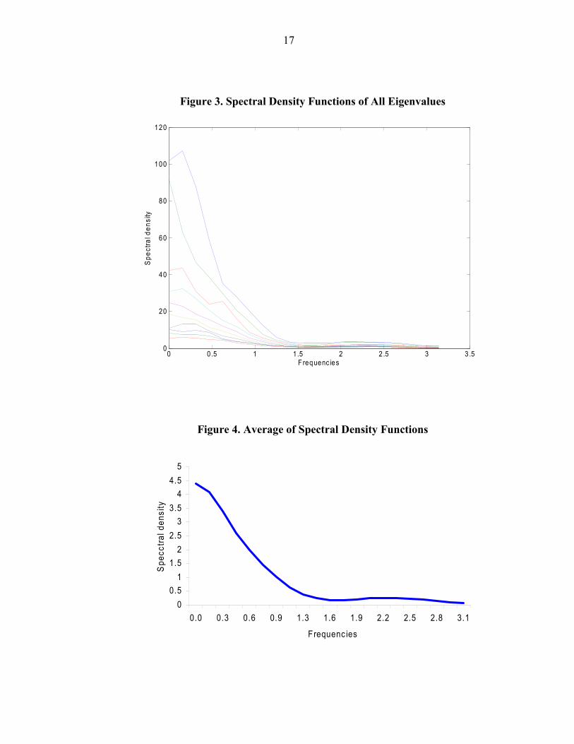
17

Figure 3. Spectral Density Functions of All Eigenvalues

0 0.5 1 1.5 2 2 .5 3 3 .50

20

40

60

80

100

120

Frequenc ies

Spe

ctra

l den

sity

Figure 4. Average of Spectral Density Functions

00.5

11.5

22.5

33.5

44.5

5

0.0 0.3 0.6 0.9 1.3 1.6 1.9 2.2 2.5 2.8 3.1

Frequenc ies

Spe

cctra

l den

sity

18

B. Properties of the Coincident Indicator

The proposed indicator must meet the following three criteria to be economically meaningful indicator in explaining the GCC area business cycle:12

(i) cross-sectional smoothing:

The idiosyncratic component of each variable captures both the variable-specific shocks (i.e., shocks to specific industry), and local-specific shocks (i.e., shocks affect only a specific region). These two kinds of shocks should not explain a large fraction of the real GCC GDP growth since the aggregation process minimizes the idiosyncratic component. These shocks should be monitored by sectoral and local policy makers. On the other hand, policymakers at the GCC supernational monetary agency should focus on monitoring only the common shocks, which affect the GCC-wide economic developments. Furthermore, the idiosyncratic component also captures measurement errors, because the GDP data are obtained by estimation procedures, not by direct observation, and they are also aggregated from heterogeneous sources. These errors are cross-sectional weakly correlated. Therefore, the coincident indicator of GCC business cycle should be free from all sources of idiosyncratic variations.

(ii) intertemporal smoothing:

Since the common component of any variable is stationary, then it can be decomposed into the sum of waves of different periodicity. That is, the common component can be represented as the sum of a cyclical component, C

itχ , represented by smooth waves with long and

medium-run periodicity, and a non-cyclical component, NCitχ , represented by waves with

short-run periodicity such as seasonal and high-frequencies volatility. The coincident index should be washed out from a non-cyclical component.

(iii) updating:

In order for the proposed indicator to be a useful tool, it has to provide policymakers with timely information about the GCC-wide economic developments. At every time t, common factors have to be estimated in order to construct the common components. However, since not all data will be available at time t or even for 1t − , then some variable have to be forecasted.13 Therefore, the coincident indicator will be subject to small revision after short period as new data release. Clearly there is a prediction error contained in the estimated indicator; however, the GDFM can reduce it by exploiting the information coming from the cross-section variables (especially the leading variables). Moreover, by classifying variables 12 See Cicconi (2005) and Altissimo et al. (2001)

13 For full explanation of the procedures, see Altissimo et al. (2001).

19

into leading, coincident, or lagging with respect to the reference cycle, we can use the leading variables to explain the likely development of the coincident indicator.

C. The Construction of a Coincident Indicator

The estimation procedures of the coincident indicator consist of three steps. The first step consists of estimating the covariance matrices of the common and idiosyncratic components. The second step consists of estimating the static factors. These steps are the two-step estimation procedures of Forni et al. (2005), which are described in section II. The final step consists of estimating the cyclical component of the GCC GDP growth, 1

Ctχ , by projecting

1Ctχ onto the leads and lags of the static factors (i.e. projecting 1

Ctχ onto ,..., ,...,t m t t m− +v v v ).

The projection coefficients derived by the covariance matrices of the cyclical components and not from the OLS estimation. Formally, set ,..., ,..., )t m t t m− +tV = (v v v ,

x x

x x

x x

n r n r

n r n r

n r n r

⎛ ⎞⎜ ⎟⎜ ⎟=⎜ ⎟⎜ ⎟⎜ ⎟⎝ ⎠

Z 0 00 Z 0

W

0 0 Z

L

L

M M O M

L

and ( ... ... )t t m t t m+ −′ ′ ′ ′=Y y y y , then t t=V WY . The sample covariance matrix of tY can be represented as:

(0) (1) (2 )(1) (0) (2 1)

(2 ) (2 1) (0)

mm

m m

⎛ ⎞⎜ ⎟′ −⎜ ⎟=⎜ ⎟⎜ ⎟⎜ ⎟′ ′ −⎝ ⎠

Γ Γ ΓΓ Γ Γ

M

Γ Γ Γ

L

L

M M O M

L

and ( )Ct tE ′ =χ Y R , where

( ( ) ... (0) ... ( ))C C Cm mχ χ χ′ ′ ′=R Γ Γ Γ

Finally, to estimate the cyclical components, we project Ctχ on tV :

1( )Ct t

−′ ′=χ RW W MW W Y (16)

There is one problem with the estimates of (16), that is, t h+y is not available for 0h > . To

solve the mentioned problem, we substitute the forecast of the common components, T h+χ , from (15) in place of t h+y , and then apply equation (16).14

14 For more details on the treatment of the end-of-sample unbalance, see Altissimo et al.(2001)

20

Figure 5 shows the coincident indicator for the GCC area estimated with quarterly data over the period 1981.Q1 to 2007.Q2. Because the indicator coincides with a “growth cycle” definition, a positive value of the coincident index signals a period of growth above the long-run growth rate, and vice versa. The indicator can be naturally interpreted as the quarterly growth rate of the real GDP in the GCC area. Figure 5 also compares the extracted coincident indicator to the actual quarterly growth rate of real GDP in the GCC area. With the exception of the early 1980s and during the first Gulf War (1990–1991), the figure clearly shows how the coincident indicator closely tracks the movements of the GDP growth for the GCC area. Indeed, their correlation over the whole sample is around 87 percent.

Figure 5. The GCC Coincident Indicator and the GCC Area GDP Growth Rate

-15

-10

-5

0

5

10

15

1982

1984

1986

1988

1990

1992

1994

1996

1998

2000

2002

2004

2006

P ercentCoinc ident Indicator GDP growth

To compare the coincident indicator with respect to countries in the GCC area, Figure 6 reports the behavior of each country-common component against the coincident indicator. It should be noted that the former should not be interpreted as national indicators since they do not contain a nation specific component. It can be interpreted as the part of the national cycle that is common across all of the GCC economies. With the exception of Bahrain and Oman, there is close comovement between the common component of the GDP growth for each country and the GCC area coincident indicator. This is not surprising since both Bahrain and Oman are the two most diversified economies (less dependent on hydrocarbon income) in the GCC area, and their weights in the GCC GDP are the smallest. Moreover, both Bahrain and Oman have been using their limited oil revenues to diversify their economic structures and develop the private sector. For example, Bahrain is trying to support the private sector by developing a high-tech service industry, whereas Oman is trying to support both the gas and tourism industries. In contrast, the common components of GDP growth in Qatar and UAE have over-performed the GCC area at the end of the sample. This is due to the fact that both of these countries have been enjoying a high record of public and private investments, especially in the financial sector, tourism infrastructures, and real-estate sector.

21

Figure 6. The GCC Coincident Indicator and the Common Component of National GDP

Growth

-15

-10

-5

0

5

10

15

1982

1984

1986

1988

1990

1992

1994

1996

1998

2000

2002

2004

2006

P ercentCoinc ident Indicator Qatar

-15

-10

-5

0

5

10

15

1982

1984

1986

1988

1990

1992

1994

1996

1998

2000

2002

2004

2006

P ercentCoinc ident Indicator United A rab Em irates

-10-8-6-4-202468

10

1982

1984

1986

1988

1990

1992

1994

1996

1998

2000

2002

2004

2006

P ercentCoinc ident Indicator S audi A rabia

22

Figure 7. The GCC Coincident Indicator and the Common Component of National GDP Growth

-60-50-40-30-20-10

010203040

1981

1984

1987

1990

1993

1996

1999

2002

2005

P ercentCoinc ident Indicator Kuwait

-8-6-4-202468

10

1982

1984

1986

1988

1990

1992

1994

1996

1998

2000

2002

2004

2006

P ercentCoinc ident Indicator Bahrain

-10

-5

0

5

10

15

20

1982

1984

1986

1988

1990

1992

1994

1996

1998

2000

2002

2004

2006

P ercentCoinc ident Indicator Om an

23

V. DEGREE OF COMMONALITY AND CYCLICAL BEHAVIOR OF THE VARIABLES

A. Degree of Commonality

As it is shown in Section II, each time series can be decomposed into two components: the common component and the idiosyncratic component. Formally, we can measure the business cycle information contained in each variable by:

( )( )

Ci

ii

varCvar y

χ= (17)

where iC represents the degree of commonality of variable i. Appendix Table 1 in Appendix I shows the degree of commonality for each variable in the dataset. Averaging over cross-sectional units, the cyclical common components explain almost 40 percent of the series’ total variance. This result is in line with Cristadoro et al. (2005) and Altissimo et al. (2001). The degree of commonality of economic variables ranges between 65 percentand 11 percent. For the key variable of interest, the commonality ratio of the GCC GDP growth is 57 percent. Also, by examining the degree of commonality of all variables in the dataset, it is easy to see that nominal effective exchange rates, oil prices, consumer prices, oil productions, imports, exports, net foreign assets, and monetary aggregates have greater commonality ratios compared to interest rates and yield spreads. As a by-product of utilizing the GDFM, we can categorize the cyclical behavior of each macroeconomic variable with respect to the reference cycle as pro-cyclical or counter-cyclical. We can then re-categorize each variable as a lagging, coincident, or leading variable against the reference cycle. It is important to first determine the relevant reference cycle. As it was mentioned in Section IV, the GDP figures are viewed as a broad measure of the aggregate economic activity. Thus, in this paper, the reference cycle is defined as the common component of the GCC GDP growth at the cyclical business cycle periodicities.

To determine the direction and timing of each time series, I first computed the cross-spectral density of each common component with respect to the reference cycle, , ( )i GDPσ θ . Then, to classify each time series as pro-cyclical or counter-cyclical, I computed the phase angle shifts of each variable with respect to the reference cycle at the zero frequency, , (0)i GDPφ . A

variable is classified as pro-cyclical if , (0) 0i GDPφ = (positive long-term correlation), and as

counter-cyclical if , (0)i GDPφ π= (negative long-term correlation). Grouping time series by sector, Table 1 shows the majority of the series in the dataset (60 percent) are classified as pro-cyclical variables with respect to the reference cycle, whereas the remaining are classified as counter-cyclical.15

15 Detailed results for each variable in the dataset can be found in Appendix Table 1.

24

Table 1. The Direction and Timing of Variables Against the Coincident Indicator

Variable Direction Timing

Industrial Production Pro-cyclical Coincident Domestic GDP Pro-cyclical Coincident Foreign GDP Euro area Pro-cyclical Leading

U.S. Counter-cyclical Coincident

Financial Variables Interest rates Pro-cyclical Coincident

Yield spread Counter-cyclical Leading

Nominal effective exchange rates Counter-cyclical Leading

Prices GCC consumer prices Pro-cyclical Lagging & coincident Real oil prices Pro-cyclical coincident Monetary Aggregates

Money supply Counter-cyclical Leading

Net claim on government Counter-cyclical Leading

Total international reserves Pro-cyclical Coincident International trade Exports Pro-cyclical Coincident Imports Pro-cyclical Lagging

Having split the variables into either pro-cyclical or counter-cyclical variables, I can further split these two groups as lagging, coincident, or leading variables by calculating the time lag

at the business frequency, ,,

( )( ) i GDP

i GDP

φ θψ θ

θ= . The time lag is calculated at a frequency

2

5

πθ = , where I assume an average length of the business cycle to be more than five quarters.

A variable is classified as lagging when the time lag is lower than -1 (quarter), leading when it is more than 1, and coincident otherwise. Out of 82 series, Table 1 shows 18 percent lagging, 55 percent to be coincident, and 27 percent to leading.

B. Business Cycle: Stylized Facts

In this section, I analyze by sector the cyclical behavior of economic variables with respect to the reference cycle.

25

Production

The industrial production indices (petroleum production index and oil production level) exhibit strong comovement within the cross-section time series, where almost 40 percent of their variation can be explained by the first three common dynamic factors. Since the level of industrial production is a narrower measure of the overall aggregate economic activity, the direction and timing of industrial production tend to coincide with the reference cycle. Further, all industrial production indices are pro-cyclical and coincident; that is, they tend to rise when GDP growth rises, and fall when GDP growth declines. The Gross Domestic Product for each of the economies in the GCC area, with the exception of Oman, exhibits a pro-cyclical and coincident behavior with respect to the reference cycle. The average explained variance by the first three common factors at cyclical frequencies is almost 50 percent. The direction and timing of the Foreign Gross Domestic Product does not reveal a systemic behavior with respect to the reference cycle. While Euro area GDP is procyclical and leading, the U.S. and Japan GDP are countercyclical and coincident. That is, the movement in the Euro area economies gives some signals as to how the GCC business cycle is likely to develop. The previous result is supported by the fact that the Euro area is a closer trade partner than the United States. By examining the Direction of Trade Statistic (DOTS) for the GCC area, it can be noticed that exports of the GCC area to the Euro area are almost twice as much as those to the United States for most of the sample from 1980 to 2006. Another possible explanation of the counter-cyclical behavior between the GCC area and the U.S. GDP is through the adopted fixed exchange rate regimes in the GCC region. To explain the exchange rate channel, assume that the U.S. economy is going through a slowdown. The Federal Reserve Bank will ease the monetary policy by lowering the interest rate in order to stimulate the U.S. economy. As a result, the GCC central banks will lower their interest rates in order to maintain the fixed exchange rate regimes. While the slowdown in the U.S. economy will have a negative effect on the GCC GDP by reducing the demand for oil, the reduction in interest rates will have a positive effect by stimulating the GCC economies. It is most likely that the effect of interest rates will offset the lower demand by the U.S. since the interest rates pass-through channel is faster than the change in the elasticity of oil demand.

Financial Variables

The interest rates (deposit rate and lending rate) for the GCC area are pro-cyclical and coincident with respect to the reference cycle. Due the fixed exchange rate regimes in the GCC area, the nominal interest rates coincide also with the movement in the U.S. Treasury bill rate, as implied by Uncovered Interest Parity (UIP).

26

The yield spread, which is defined as long-term (corporate bond) interest rate minus short-term (government bond) interest, is usually positive and slopes upward to reflect the liquidity premium. If it starts to flatten or invert, it is most likely to signal an increasing possibility of coming recessions as the monetary policy starts to tighten. Hamilton and Kim (2002) show evidence of how the yield curves flatten or invert prior to all eight U.S. recessions between 1953 and 1998. Therefore, yield spreads are a good predictive signal of the future aggregate activity. The U.S. government yield spread and corporate yield spread appear to be counter-cyclical and leading with respect to the GCC reference cycle. This result confirms our previous result of the opposite movement between the GCC reference cycle and the U.S. GDP. The nominal effective exchange rates are clearly counter-cyclical and leading by two quarters. Similar to the yield spreads, the movements of the exchange rates provide good signals about the underlying direction of the reference cycle. In conclusion, the leading property of most of the financial variables is in accordance with the economic literature, where financial asset prices reflect market expectations about future economic outcomes. Prices

The average explained variance of the first three common factors of GCC consumer prices is around 40 percent. More than 67 percent of consumer prices are procyclical. The timing of consumer prices with respect to the reference cycle is mixed. While 50 percent of consumer prices appear to be lagging, the remaining coincide with the reference cycle. The existence of some lagging consumer prices is not surprising if we assume that some nominal frictions, such as price stickiness, exist. With regard to the oil prices, it is not surprising to find a clear picture of its cyclical behavior. Since the GCC area is heavily dependent on the oil revenues, the movement of oil prices is procyclical and coincident with the reference cycle. The foreign consumer prices in the Euro area, Japan, and the United States appear to be countercyclical and leading with respect to the reference cycle. As the foreign consumer prices start to rise, the currencies of the GCC economies depreciate in real term, which causes exports to increase. As a result, the GCC GDP starts to increase due to the positive effect of the net exports. The leading time of foreign consumer prices vary from one quarter and a half to two quarters and a half. Monetary Aggregates

In macroeconomic literatures, the cyclical behavior of money supply with respect to the aggregate economic activity is controversial. In the seminal work of Friedman and Schwartz (1963), they analyzed the money supply behavior for over a century. They concluded that

27

money supply tended to be pro-cyclical and leading. Since the GCC economies have fixed exchange regimes against the U.S. dollar, money supply is determined exogenously by the U.S. Federal Reserve Bank (i.e., monetary policy in the GCC area is passive). The money supply measure used in this paper is M2. It exhibits a counter-cyclical and leading behavior with the reference cycle. If the money supply is procyclical and leading in the United States, then the countercyclical behavior of the money supply in the GCC area is consistent with our previous findings that the U.S. GDP is counter-cyclical to the GCC reference cycle. The net claim on central governments, defined as claim on central government by banks minus central government deposit at the central bank, shows consistent cyclical behavior pattern with respect to the reference cycle. In most cases, they are countercyclical and leading (Bahrain and United Arab Emirates are lagging). This result is not surprising since all of the oil companies in the GCC area are owned by the central governments. Thus, as oil revenues accumulate over time, the central governments start to decrease their debt positions with the private banks. The total international reserves, defined as foreign exchange plus SDR and the reserve position at the International Monetary Fund, appear to be procyclical and coincident with respect to the reference cycle. Only Bahrain and Kuwait show countercyclical behavior. The procyclical behavior of the international reserve is explained by the fact that oil revenues come in the form of the U.S. dollars, since oil is quoted in the commodity markets in U.S. dollars. International Trade

The cyclical behavior of exports and imports show a clear-cut pattern. While exports are procyclical and coincident, imports are procyclical and lagging. Since the GCC economies are oil-based economies, then as oil exports rise, so does the GDP. As a result of increasing GDP, governments and private sectors increase their spending, which causes imports to rise. While the export sector coincides with the reference cycle, the import sector lags the reference cycle as both governments and private spending take some time to reflect the rise in the GDP.

VI. OBSERVED ECONOMIC VARIABLES AND LATENT FACTORS

In many economic theories, it has been found that a small set of common factors explain a large part of variation in cross-section variables. For instance, the Capital Asset Pricing Theory (CAPM) assumes that the variation in all assets returns can be explained by a one systemic common factor, which is the market return. Similarly, the Arbitrage Pricing Theory (APT) is a generalized version of CAPM. It assumes that a small set of common factors can explain most of the variation in all assets returns. The previous two examples do not give an explicit definition of the number of common factors. Also, they do not specify the observed counterpart variables of these common factors in order to conduct empirical testing of these theories.

28

With the advancement of modeling and estimating factor models, many of the empirical applications have tried to replace the theoretical unobserved common factors with the statically extracted factors. For example, in this paper, the unobserved common factors in the common component are replaced by the estimated statistical dynamic common factors from the GDFM.

The drawback of this procedure is that the estimated statistical common factors do not have any economic interpretation. To overcome this problem, Bai and Ng (2006) propose a test to compare if the individual observed variables and the latent factors are approximately the same. The proposed two statistics are:

( )( )

ˆvar ( )( )

ˆvar ( )j

NS jj

=εy

(18)

( )( )

2 ˆvar ( )( )

var ( )j

R jj

=yy

(19)

where ˆ( )jε is the measurement error obtained after subtracting the individual observed variables ( )jy from the estimated observed variables ˆ ( )jy . The latter is obtained by

regressing the individual observed variables on the latent factors, i.e. ˆˆ jt j ty β= F , where ˆjβ is

obtained by the least squares method, and tF is obtained from the GDFM. The first statistic, (18), represents the noise-to-signal ratio; that is, the larger NS(j) is, the more departed are the observed variables from the latent factors. In the extreme case, if the ˆ ( )jy is exactly the same as the latent factors, then NS(j) is equal to zero. The second statistic, (19), is simply the coefficient of determination. If 2 ( )R j is one, then the individual observed variables is an exact latent factor. For the second statistic to be meaningful, it is important to obtain a confidence interval for 2 ( )R j . The upper and lower confidence interval is given by:

( ) ( ) ( )2 22 2 2 2

2 1 2 1, 2*1.96 , 2*1.96j j j j

j j j j

R R R RR R R R

T T+ −

⎛ ⎞− −⎜ ⎟= + −⎜ ⎟⎝ ⎠

(20)

The results of the proposed two statistics are summarized by sector in Table 2. Many surprising features emerge from Table 2.16 First of all, it is easy to see that nominal variables (such as nominal effective exchange rates, monetary aggregates, and consumer prices) are strong proxies for the latent factors. Specifically, the nominal effective exchange rates shocks have the strongest relations with the unobserved common factors, where NS and 2R are

16 Detailed results for each variable in the dataset can be provided by the author.

29

0.17 and 85 percent, respectively. Similarly, the consumer prices in the GCC area and the consumer prices in foreign economies appear to have strong relation to the latent factors. Second, the GCC GDP is also a good proxy of the latent factors with 2R around 55 percent. Finally, exports and oil productions unexpectedly are not good proxies for the latent factors. This puzzling result comes from the fact that the GCC area is comprised of natural-resource-based economies; therefore, it is expected that real shocks ought to play a vital role in the business cycle fluctuations. However, there is hardly any evidence of strong relation between oil productions and latent factors.

The previous results imply that the main source of economic fluctuations in the panel of macroeconomic variables is the nominal shocks. These nominal shocks appear to be more important than real shocks in explaining the driving forces of business cycle evolutions in the GCC area.

Table 2. Testing the Observed Macroeconomic Data Against the Latent Factors

Descriptor NS(j) 2 ( )R j Nominal Effective Exchange rates 0.17 85% GCC GDP 0.82 55% Europe CPI 0.86 54% US CPI 1.21 45% Money Supply 2.43 34% Net Foreign Assets 2.97 32% Japan CPI 2.18 31% Consumer Prices 2.74 31% US GDP 2.30 30% Exports 4.01 25% Oil Prices 3.29 23% Treasury Bill 3.64 22% Net Claim on Central Governments 7.16 20% Interest rates 6.72 16% Total Reserves 7.27 16% U.S. government yield spread 5.60 15% EU 15 GDP 7.22 12% Imports 10.84 12% Oil Productions 9.01 11% Japan GDP 39.46 2% corporate yield spread 44.30 2% *The statistics in this table are the average results by sector for individual time series.

VII. CONCLUSION

By establishing a single currency in the Gulf Cooperation Council (GCC) area in 2010, policymakers at the prospective supernational monetary agency will need to decide on a common monetary policy based on the GCC-wide economic developments. Having timely information about the development of the GCC business cycle is invaluable for the

30

policymakers. Since the GDP data is released with considerable lag and contains measurement errors and seasonal effects, constructing a smoother and timely indicator of the GCC business cycle can be a good analytical and empirical tool for the policymakers and the business community. It provides a clear signal about the underlying movement of the GCC area economy. The coincident indicator is constructed by utilizing the Generalized Dynamic Factor Model (GDFM) proposed by Forni et al. (2000, 2004, and 2005), and applied to the Euro area by Altissimo et al. (2001). The GDFM is applied to a quarterly dataset with 82 economic variables from 1980 to 2007.

The results suggest that as few as three common shocks can be sufficient in explaining business cycle developments for the GCC area. The constructed coincident indicator closely resembles the movement in the GCC GDP growth, especially for the last ten years, pointing to a higher degree of commonality across the GCC economies. As a by-product of utilizing the GDFM, a higher degree of commonality is found within nominal effective exchange rates, exports, imports, oil prices, oil productions, consumer prices, and monetary aggregates, since those variables are closely related to the GCC GDP (which depends to a great extent on oil income). The direction and timing of economic variables is mixed. While oil prices, consumer prices, exports, imports, and oil productions are procyclical with respect to the coincident indicator, nominal effective exchange rates behave in the opposite way to the reference cycle. Further, in accordance with the economic theory, financial variables such as exchange rates, interest rates, and yield spreads are classified as leading variables with respect to the reference cycle, which reflect the expectation of the future economic outcomes. On the other hand, a high proportion of the lagging variables are found within consumer prices and imports. This result suggests that some nominal frictions, such as price stickiness, exist in the GCC area.

Finally, to test the economic meaningfulness of the statistically latent factors, the proposed test by Bai and Ng (2006) was applied to the GCC dataset. The results show that the nominal shocks are strong proxies for the latent factors. These nominal shocks appear to be more important than real shocks in explaining the driving forces of business cycle evolutions in the GCC area.

31

APPENDIX I: DATA SET

Appendix Table 1: Data, Degree of Commonality, and Cyclical Behavior Country Descriptor Commonality Phase Time lagGCC Real Gross Domestic Product 0.57 0.00 (0.00) BHR Real Gross Domestic Product 0.21 0.00 (0.84) KWT Real Gross Domestic Product 0.53 0.00 (0.14) OMN Real Gross Domestic Product 0.49 3.14 (1.87) QTR Real Gross Domestic Product 0.36 0.00 0.01 KSA Real Gross Domestic Product 0.44 0.00 0.07 UAE Real Gross Domestic Product 0.36 0.00 (0.01) BHR Nominal Effective Exchange Rate 0.53 3.14 2.16 OMN Nominal Effective Exchange Rate 0.51 3.14 2.36 QTR Nominal Effective Exchange Rate 0.48 3.14 2.16 KSA Nominal Effective Exchange Rate 0.46 3.14 2.34 UAE Nominal Effective Exchange Rate 0.50 3.14 2.17 BHR Consumer Price Index 2000=100 0.42 3.14 (1.88) KWT Consumer Price Index 2000=100 0.50 3.14 (1.86) OMN Consumer Price Index 2000=100 0.30 0.00 (0.78) QTR Consumer Price Index 2000=100 0.46 0.00 (0.41) KSA Consumer Price Index 2000=100 0.23 0.00 (1.02) UAE Consumer Price Index 2000=100 0.27 0.00 (0.62) Average Oil Prices 0.38 0.00 (0.74) BHR Money plus Quasi-Money 0.22 3.14 (2.01) KWT Money plus Quasi-Money 0.51 3.14 2.01 OMN Money plus Quasi-Money 0.59 3.14 2.47 QTR Money plus Quasi-Money 0.37 0.00 1.53 KSA Money plus Quasi-Money 0.53 3.14 (1.46) UAE Money plus Quasi-Money 0.45 3.14 (0.73) BHR Foreign Assets (Net) 0.36 3.14 0.85 KWT Foreign Assets (Net) 0.22 3.14 1.45 OMN Foreign Assets (Net) 0.33 3.14 (2.31) QTR Foreign Assets (Net) 0.20 0.00 1.28 KSA Foreign Assets (Net) 0.64 0.00 (0.23) UAE Foreign Assets (Net) 0.25 3.14 (0.19) BHR Claims on Private Sector 0.38 0.00 (0.45) KWT Claims on Private Sector 0.30 3.14 1.76 OMN Claims on Private Sector 0.28 3.14 2.17 QTR Claims on Private Sector 0.26 0.00 (0.98) KSA Claims on Private Sector 0.39 0.00 (0.39) UAE Claims on Private Sector 0.56 0.00 (0.50) BHR Total International Reserves 0.30 3.14 0.61 KWT Total International Reserves 0.16 3.14 2.07 OMN Total International Reserves 0.22 0.00 2.50 QTR Total International Reserves 0.18 0.00 0.17 KSA Total International Reserves 0.11 0.00 (0.17) UAE Total International Reserves 0.16 0.00 0.54 BHR Exports 0.38 0.00 (0.19) KWT Exports 0.54 0.00 (0.58) OMN Exports 0.34 0.00 0.33 QTR Exports 0.33 0.00 (0.31)

32

Country Descriptor Commonality Phase Time lagKSA Exports 0.52 0.00 (0.14) UAE Exports 0.51 0.00 (0.05) BHR Imports 0.39 0.00 (0.51) KWT Imports 0.43 0.00 (1.40) OMN Imports 0.36 0.00 0.24 QTR Imports 0.26 0.00 (1.29) KSA Imports 0.32 0.00 (1.30) UAE Imports 0.24 0.00 (1.81) BHR Crude Petroleum Production Index 2000=100 0.27 0.00 0.23 KWT Crude Petroleum Production Index 2000=100 0.42 0.00 0.09 OMN Crude Petroleum Production Index 2000=100 0.26 3.14 1.03 QTR Crude Petroleum Production Index 2000=100 0.32 0.00 (0.20) KSA Crude Petroleum Production Index 2000=100 0.47 0.00 0.04 UAE Crude Petroleum Production Index 2000=100 0.34 0.00 0.45 KWT Oil production 0.49 0.00 (1.15) QTR Oil production 0.30 0.00 (0.61) KSA Oil production 0.47 0.00 (0.13) UAE Oil production 0.34 0.00 (0.36) Japan Real Gross Domestic Product 0.22 3.14 0.81 U.S. Real Gross Domestic Product 0.37 3.14 0.45 EU 15 Real Gross Domestic Product 0.19 0.00 1.86 Japan Consumer Price Index 2000=100 0.41 3.14 1.45 U.S. Consumer Price Index 2000=100 0.46 3.14 2.07 EU 15 Consumer Price Index 2000=100 0.51 3.14 (2.39) U.S. Treasury Bill 0.35 0.00 0.03 U.S. Government yield spread 0.18 3.14 2.49 U.S. Corporate yield spread 0.14 3.14 2.43 GCC Deposit rate 0.26 0.00 0.28 GCC Lending rate 0.15 0.00 (0.23) BHR Claims on Central Government (Net) 0.15 0.00 (1.51) KWT Claims on Central Government (Net) 0.27 3.14 (0.93) OMN Claims on Central Government (Net) 0.28 3.14 0.81 QTR Claims on Central Government (Net) 0.29 3.14 1.94 KSA Claims on Central Government (Net) 0.64 3.14 1.43 UAE Claims on Central Government (Net) 0.16 3.14 (1.95)

1) GCC is the Gulf Cooperation Council, BHR is Bahrain, KWT is Kuwait, OMN is Oman, QTR is Qatar, KSA is the Kingdom of Saudi Arabia, and UAE is the United Arab Emirates.

2) The commonality of any time series is the relative ratio of its common component variance to its total variance. 3) Phase determines the direction of the time series with respect to the reference cycle. The time series is pro-cyclical if the

phase is equal zero, otherwise it is counter-cyclical. 4) The variable is lagging if time lag < -1, leading > 1, otherwise coincident.

33

REFERENCES Altissimo, F., A. Bassanetti, R. Cristadoro, M. Forni, M. Hallin, M. Lippi, et al., 2001,

EuroCOIN: A Real Time Coincident Indicator of the Euro Area Business Cycle (Publication no. 3108). from CEPR: http://www.cepr.org/pubs/new-dps/dplist.asp?dpno=3108&action.x=15&action.y=4&action=ShowDP

Bai, J., and S. Ng, 2002, “Determining the Number of Factors in Approximate Factor

Models,” Econometrica, 70(1), pp. 191–221. Bai, J., and S. Ng, 2006, “Evaluating Latent and Observed Factors in Macroeconomics and

Finance,” Journal of Econometrics, 131(1–2), pp. 507–537. Boivin, J., & S. Ng, 2006, “Are More Data Always Better for Factor Analysis?,” Journal of

Econometrics, 132(1), pp. 169–194. Brillinger, D. R., 1981, Time Series : Data Analysis and Theory (Expanded ed.), San

Francisco: Holden-Day. Burns, A. F., and W.C. Mitchell, 1946, Measuring Business Cycles, New York: National

Bureau of Economic Research. Chamberlain, G., 1983, “Funds, Factors, and Diversification in Arbitrage Pricing Models,”

Econometrica, 51(5), pp. 1305–1323. Chamberlain, G., and M. Rothschild, 1983, “Arbitrage, Factor Structure, and Mean-Variance

Analysis on Large Asset Markets,” Econometrica, 51(5), pp. 1281–1304. Cristadoro, R., M. Forni, L. Reichlin, and G. Veronese, 2005, “A Core Inflation Indicator for

the Euro Area,” Journal of Money, Credit, and Banking, 37(3), pp. 539–560. Forni, M., M. Hallin, M. Lippi, and L. Reichlin, 2000, “The Generalized Dynamic-Factor

Model: Identification and Estimation,” Review of Economics and Statistics, 82(4), pp. 540–554.

Forni, M., M. Hallin, M. Lippi, and L. Reichlin, 2004, “The Generalized Dynamic Factor

Model Consistency and Rates,” Journal of Econometrics, 119(2), pp. 231–255. Forni, M., M. Hallin, M. Lippi, and L. Reichlin, 2005 “The Generalized Dynamic Factor

Model: One-Sided Estimation and Forecasting,” Journal of the American Statistical Association, 100(471), pp. 830-840.

Forni, M., and M. Lippi, 2001, “The Generalized Dynamic Factor Model: Representation

Theory,” Econometric Theory, 17(6), pp. 1113–1141. Friedman, M., and A.J. Schwartz, 1963, A Monetary History of the United States, 1867–

1960, Princeton: Princeton University Press.

34

Geweke, J., 1977, The Dynamic Factor Analysis of Economic Time Series Models. Paper presented at the Latent Variables in Socio-Economic, Amsterdam.

Giannone, D., L. Reichlin, and L. Sala, 2002, “Tracking Greenspan: Systematic and

Unsystematic Monetary Policy Revisited.” Giannone, D., L. Reichlin, and L. Sala, 2004, “Monetary Policy in Real Time,” NBER

Macroeconomics Annual, pp. 161–200. Gomez, V., and A. Maravall, 1998, “Guide for Using the Programs TRAMO and SEATS”

(Beta Version: December 1997). 44. Hamilton, J.D., and D.H. Kim, 2002, “A Reexamination of the Predictability of Economic

Activity Using the Yield Spread,” Journal of Money, Credit, and Banking, 34(2), pp. 340–360.

Sargent, T.J., and C.A. Sims, 1977, “Business cycle modeling without pretending to have too

much a priori economic theory.” Schneider, M., and M. Spitzer, 2004, “Forecasting Austrian GDP using the generalized

dynamic factor model,” [Electronic Version] from http://www.oenb.at/de/img/wp89_1__tcm14-20424.pdf