a combined fourth-order compact scheme …etna.mcs.kent.edu/vol.39.2012/pp32-45.dir/pp32-45.pdf ·...

Electronic Transactions on Numerical Analysis.Volume 39, pp. 32-45, 2012.Copyright 2012, Kent State University.ISSN 1068-9613.

ETNAKent State University

http://etna.math.kent.edu

A COMBINED FOURTH-ORDER COMPACT SCHEME WITH ANACCELERATED MULTIGRID METHOD FOR THE ENERGY EQUATION IN

SPHERICAL POLAR COORDINATES ∗

T. V. S. SEKHAR†, R. SIVAKUMAR‡, S. VIMALA †, AND Y. V. S. S. SANYASIRAJU§

Abstract. A higher-order compact scheme is combined with an accelerated multigrid method to solve the energyequation in a spherical polar coordinate system. The steady forced convective heat transfer from a sphere which isunder the influence of an external magnetic field is simulated. The convection terms in the energy equation arehandled in a comprehensive way avoiding complications in the calculations. The angular variation of the Nusseltnumber and mean Nusselt number are calculated and compared with recent experimental results. Upon applying themagnetic field, a slight degradation of the heat transfer is found for moderate values of the interaction parameterN,

and for high values ofN an increase in the heat transfer is observed leading to a nonlinear behavior. The speedyconvergence of the solution using the multigrid method and accelerated multigrid method is illustrated.

Key words. higher-order compact scheme, accelerated multigrid method, forced convection heat transfer, ex-ternal magnetic field

AMS subject classifications.65N06, 65N55, 35Q80

1. Introduction. The development of numerical methods for solving the Navier-Stokesequations is progressing from time to time in terms of accuracy, stability, and efficiency inusing less CPU time and/or memory. It is well-known that at least second-order accuratesolutions are required to capture flow phenomena such as boundary layer, vortices etc., whilesolving Navier-Stokes equations at high values of the Reynolds numbers (Re). The centraldifference scheme (CDS) causes nonphysical oscillations and lacks diagonal dominance inthe resulting linear system. The first-order upwind difference approximation for convectiveterms and central differences for diffusion terms makes thefinite difference scheme morestable due to artificial viscosity. Also, the diagonal dominance is assured for the linear sys-tem and so it can be solved easily using Point Gauss-Seidel orLine Gauss-Seidel, etc. Asthe convective terms are approximated by first-order upwinddifferences, the scheme is notsecond order accurate and may fail to capture the flow phenomena at high values ofRe dueto the dominance of convection. To achieve second-order accuracy, defect correction tech-niques are used [15, 29]. The second-order upwind methods are no better than the first-orderupwind difference ones at high values of the flow parameters such asRe. All these methodsrequire fine mesh grids to achieve grid independence or to getacceptable accuracy. Multigridmethods (which uses a sequence of coarser grids) are more popular in achieving fast conver-gence, which results in significant reduction of CPU time andalso makes it possible to handlea huge number of mesh points to achieve acceptable accuracy.Notable contributions usingthe multigrid approach include articles by Ghia et al. [9], Fuchs and Zhao [8], Vanka [28],and Brandt [4]. Thompson [26] described a method which combines the multigrid methodwith automatic adaptive gridding to provide the basis of a stable solution strategy in Cartesiancoordinate systems.

All the above methods may fail to capture the flow phenomena ifthe domain is too largesuch as in global ocean modeling and wide area weather forecasting applications. One ap-

∗ Received May 23, 2011. Accepted January 24, 2012. Publishedonline on March 15, 2012. Recommended byK. Burrage.

†Department of Mathematics, Pondicherry Engineering College, Puducherry-605014, India({sekhartvs, vimalaks}@pec.edu).

‡Department of Physics, Pondicherry University, Puducherry-605014, India ([email protected]).§Department of Mathematics, Indian Institute of Technology Madras, Chennai-600036, India

([email protected]).

32



HOCS COMBINED WITH MULTIGRID METHOD 33

proach to achieve accurate solutions with reduced computational costs in very large scalemodels and simulations is to use higher-order discretization methods. These methods userelatively coarse mesh grids to yield approximate solutions of comparable accuracy, relativeto the lower-order discretization methods. The conventional higher-order finite differencemethods contains ghost points and requires special treatment near the boundaries [2]. An ex-ception has been found in the high-order finite difference schemes of compact type, which arecomputationally efficient and stable and give highly accurate numerical solutions [5, 10, 20].To fully investigate the potential of using the fourth-order compact schemes for solving theNavier-Stokes equations, multigrid techniques are essential. These multigrid methods havebeen successfully used with first- and second-order finite difference methods. A preliminaryinvestigation on combining the fourth-order compact schemes with multigrid techniques wasmade by Atlas and Burrage [1] for diffusion dominated flow problems.

Multigrid solution and accelerated multigrid solution methods with fourth-order compactschemes for solving convection-dominated problems are relatively new. Some attempts havebeen made in rectangular geometry [11, 12, 17, 21, 32, 33]. However, higher order compactschemes (HOCSs) are seldom applied to flow problems in curvilinear coordinate systemssuch as cylindrical and spherical polar coordinates exceptin [13, 14, 16, 19], where compactfourth-order schemes in cylindrical polar coordinates were developed. In particular, to thebest of our knowledge, no work has been reported on high-order compact methods in spher-ical polar coordinate systems employing multigrid methods. The problem of heat transferfrom a sphere which is under the influence of an external magnetic field is also new exceptfor a few experimental results [3, 27, 31]. Fluid flow control using magnetic field (includingdipole field) has a sound physical basis which may lead to a promising technology for betterheat transfer control.

Hydromagnetic flows of electrically conducting fluids and its heat transfer have becomemore important in recent years because of many important applications including fusion tech-nology. Early experimental exploration of a magnetic control of the heat transfer is reportedby Boynton [3] in their study of magnetic heat transfer over a sphere. Uda et al. [27] ex-perimentally studied MHD effects on the heat transfer of liquid Lithium flow in an annularchannel. In their experimental study, Yokomine et al. [31] investigated heat transfer propertiesof aqueous potassium hydroxid solution (Pr ≈ 5) and concluded that there is a degradationof the heat transfer with the magnetic field. In this paper, a HOCS is employed with a com-bination of accelerated multigrid technique to solve the energy equation in spherical polarcoordinates. The forced convection heat transfer from a sphere which is under the influenceof an external magnetic field is investigated.

2. Basic equations.The forced convective heat transfer problem is formulated as steady,laminar flow in axis-symmetric spherical polar coordinates. The center of the sphere is cho-sen at the origin and the flow is symmetric aboutθ = π (upstream) andθ = 0o (downstream).The fluid is considered to be incompressible, viscous, and electrically conducting. A uniformstream from infinity,U∞, is imposed from left to right at far distances from the sphere. Themagnetic Reynolds number is assumed to be small so that the induced magnetic field can beneglected and a constant magnetic field

(2.1) H = (− cos θ, sin θ, 0)

is imposed opposite to the flow. The governing equations are the Navier-Stokes equationsand Maxwell’s equations which are expressed in non-dimensional form as follows:



34 T. V. S. SEKHAR, R. SIVAKUMAR, S. VIMALA, AND Y. V. S. S. SANYASIRAJU

∇ · q = 0

(q · ∇)q = −∇p +2

Re∇2q + N [J × H]

J = ∇× H = E + q × H

∇ · H = 0

∇× E = 0,

(2.2)

whereq is the fluid velocity,H is the magnetic field,p is the pressure,E is the electric field,J is the current density andN is the interaction parameter defined asN = σH2

∞a/ρU∞.

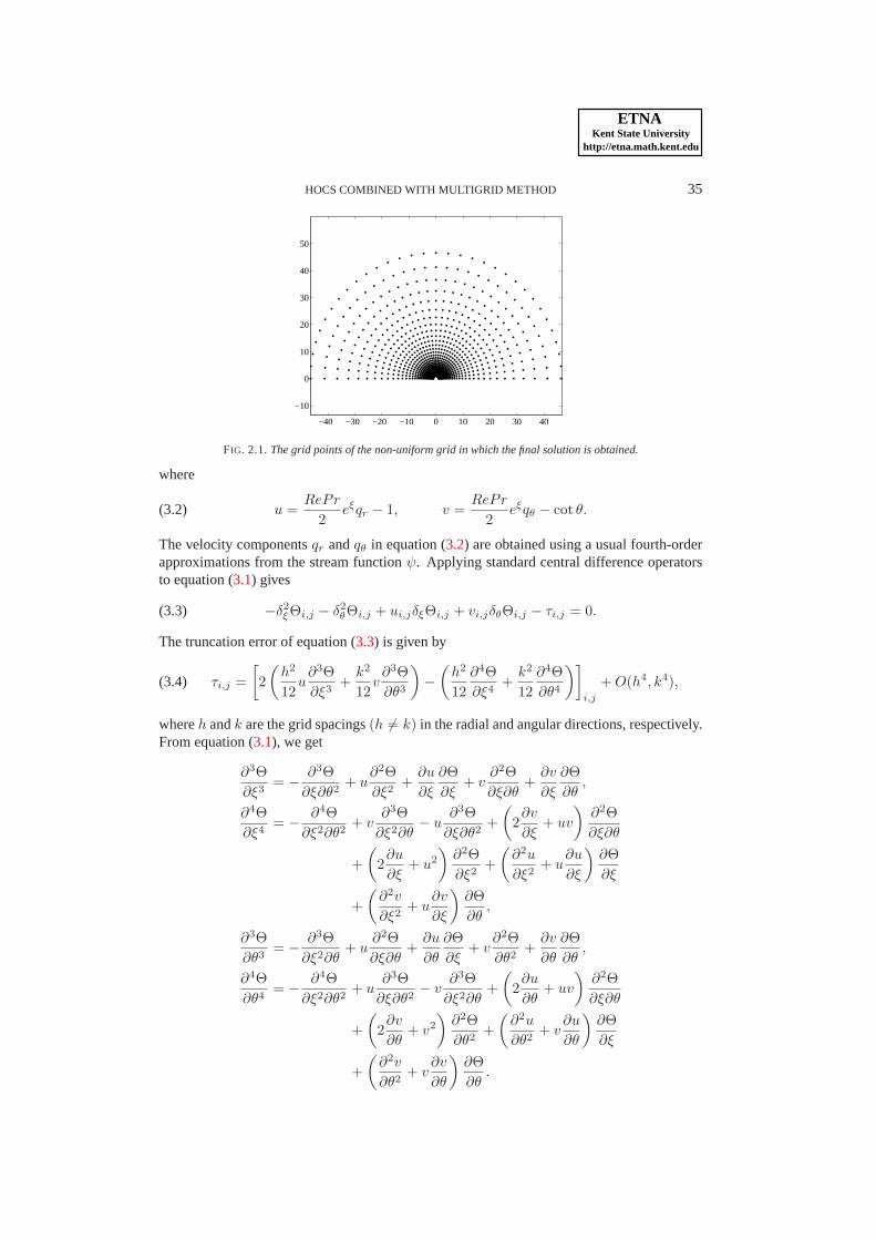
Hereσ andρ are the electric conductivity and the density of the fluid anda is the radius ofthe sphere.Re = 2aU∞/ν is the Reynolds number based on the diameter(2a) of the sphere.In order to have fine resolution near the surface of the sphere, we have used the transformationr = eξ along the radial direction, which provides the solution in the non-uniform physicalplane while keeping the uniform grid in the computational plane as shown in Figure2.1.The fluid motion is described by radial and transverse components of the velocity(qr, qθ)in a plane through the axis of symmetry, which are obtained bydividing the correspond-ing dimensional components by the main-stream velocityU∞. The velocity components areexpressed in terms of a dimensionless stream functionψ(ξ, θ) such that the equation of con-tinuity ∇ · q = 0 is satisfied. The velocity componentsqr andqθ are as follows:

(2.3) qr =e−2ξ

sin θ

∂ψ

∂θ, qθ = −

e−2ξ

sin θ

∂ψ

∂ξ.

They are obtained by solving the momentum equation expressed in the vorticity-stream func-tion formulation. The velocity field is obtained by solving equations (2.1–2.3) using a finitedifference based multigrid method followed by a defect correction technique developed bySekhar et al. [24]. The grid independent velocity components obtained from (2.1–2.3) over ahigh resolution grid512 × 512 are used to solve the energy equation. If the physical proper-ties of the fluid are assumed to be constant and the internal generation of heat by friction isneglected, the energy equation is given by

(2.4)∂2Θ

∂ξ2+

∂Θ

∂ξ+ cot θ

∂Θ

∂θ+

∂2Θ

∂θ2=

RePr

2

e−ξ

sin θ

(

∂ψ

∂θ

∂Θ

∂ξ−

∂ψ

∂ξ

∂Θ

∂θ

)

,

whereΘ(ξ, θ) is the non-dimensionalized temperature, defined by subtracting the main-flowtemperatureΘ∞ from the temperature and dividing byΘs − Θ∞. Pr is the Prandtl numberdefined as the ratio between kinematic viscosityν and thermal diffusivityκ. The boundaryconditions for the temperature areΘ = 1 on the surface of the sphere,Θ → 0 asξ → ∞,and ∂Θ

∂θ= 0 along the axis of symmetry. The numerical scheme used to solve the equations

(2.1–2.3) is described in [24], and the details of the fourth-order compact scheme to solveequation (2.4) are given in the following section.

3. Fourth-order scheme with the MG method. Both the fluid motion and the temper-ature field are axially symmetric and hence all computationshave been performed only inone of the symmetric region. The discretization of the governing equation (2.4) in the sym-metric region is done using the compact stencil. By combining the convection terms∂ψ

∂θ∂Θ

∂ξ

and ∂ψ∂ξ

∂Θ

∂θon the right-hand side of equation (2.4) with the terms∂Θ

∂ξandcot θ ∂Θ

∂θ, respec-

tively, we obtain

(3.1) −∂2Θ

∂ξ2−

∂2Θ

∂θ2+ u

∂Θ

∂ξ+ v

∂Θ

∂θ= 0,




−40 −30 −20 −10 0 10 20 30 40

−10

0

10

20

30

40

50

FIG. 2.1.The grid points of the non-uniform grid in which the final solution is obtained.

where

(3.2) u =RePr

2eξqr − 1, v =

RePr

2eξqθ − cot θ.

The velocity componentsqr andqθ in equation (3.2) are obtained using a usual fourth-orderapproximations from the stream functionψ. Applying standard central difference operatorsto equation (3.1) gives

(3.3) −δ2ξΘi,j − δ2

θΘi,j + ui,jδξΘi,j + vi,jδθΘi,j − τi,j = 0.

The truncation error of equation (3.3) is given by

(3.4) τi,j =

[

2

(

h2

12u

∂3Θ

∂ξ3+

k2

12v∂3Θ

∂θ3

)

−

(

h2

12

∂4Θ

∂ξ4+

k2

12

∂4Θ

∂θ4

)]

i,j

+ O(h4, k4),

whereh andk are the grid spacings(h 6= k) in the radial and angular directions, respectively.From equation (3.1), we get

∂3Θ

∂ξ3= −

∂3Θ

∂ξ∂θ2+ u

∂2Θ

∂ξ2+

∂u

∂ξ

∂Θ

∂ξ+ v

∂2Θ

∂ξ∂θ+

∂v

∂ξ

∂Θ

∂θ,

∂4Θ

∂ξ4= −

∂4Θ

∂ξ2∂θ2+ v

∂3Θ

∂ξ2∂θ− u

∂3Θ

∂ξ∂θ2+

(

2∂v

∂ξ+ uv

)

∂2Θ

∂ξ∂θ

+

(

2∂u

∂ξ+ u2

)

∂2Θ

∂ξ2+

(

∂2u

∂ξ2+ u

∂u

∂ξ

)

∂Θ

∂ξ

+

(

∂2v

∂ξ2+ u

∂v

∂ξ

)

∂Θ

∂θ,

∂3Θ

∂θ3= −

∂3Θ

∂ξ2∂θ+ u

∂2Θ

∂ξ∂θ+

∂u

∂θ

∂Θ

∂ξ+ v

∂2Θ

∂θ2+

∂v

∂θ

∂Θ

∂θ,

∂4Θ

∂θ4= −

∂4Θ

∂ξ2∂θ2+ u

∂3Θ

∂ξ∂θ2− v

∂3Θ

∂ξ2∂θ+

(

2∂u

∂θ+ uv

)

∂2Θ

∂ξ∂θ

+

(

2∂v

∂θ+ v2

)

∂2Θ

∂θ2+

(

∂2u

∂θ2+ v

∂u

∂θ

)

∂Θ

∂ξ

+

(

∂2v

∂θ2+ v

∂v

∂θ

)

∂Θ

∂θ.




A substitution in equation (3.4) and hence in (3.3) yields

− ei,jδ2ξΘi,j − fi,jδ

2θΘi,j + gi,jδξΘi,j + oi,jδθΘi,j

−h2 + k2

12

(

δ2ξδ2

θΘi,j − ui,jδξδ2θΘi,j − vi,jδ

2ξδθΘi,j

)

+ wi,jδξδθΘi,j = 0,

where the coefficientsei,j , fi,j , gi,j , oi,j andwi,j are given by

ei,j = 1 +h2

12

(

u2i,j − 2δξui,j

)

fi,j = 1 +k2

12

(

v2i,j − 2δθvi,j

)

gi,j = ui,j +h2

12

(

δ2ξui,j − ui,jδξui,j

)

+k2

12

(

δ2θui,j − vi,jδθui,j

)

oi,j = vi,j +h2

12

(

δ2ξvi,j − ui,jδξvi,j

)

+k2

12

(

δ2θvi,j − vi,jδθvi,j

)

wi,j =h2

6δξvi,j +

k2

6δθui,j −

(

h2 + k2

12

)

ui,jvi,j ,

and the two-dimensional cross derivativeδ operators on a uniform anisotropic mesh(h 6= k)are given by

δξδθΘi,j =1

4hk(Θi+1,j+1 − Θi+1,j−1 − Θi−1,j+1 + Θi−1,j−1)

δ2ξδθΘi,j =

1

2h2k(Θi+1,j+1 − Θi+1,j−1 + Θi−1,j+1 − Θi−1,j−1 − 2Θi,j+1 + 2Θi,j−1)

δξδ2θΘi,j =

1

2hk2(Θi+1,j+1 − Θi−1,j+1 + Θi+1,j−1 − Θi−1,j−1 + 2Θi−1,j − 2Θi+1,j)

δ2ξδ2

θΘi,j =1

h2k2

(

Θi+1,j+1 + Θi+1,j−1 + Θi−1,j+1 + Θi−1,j−1

− 2Θi,j+1 − 2Θi,j−1 − 2Θi+1,j − 2Θi−1,j + 4Θi,j

)

.

For evaluating boundary conditions along the axis of symmetry, the derivative∂Θ

∂θis approx-

imated by a fourth-order forward difference alongθ = 0 (i.e., j = 1) and a fourth-orderbackward difference alongθ = π (or j = m + 1) as follows:

Θ(i, 1) =1

25[48Θ(i, 2) − 36Θ(i, 3) + 16Θ(i, 4) − 3Θ(i, 5)]

Θ(i, m + 1) =1

25[48Θ(i, m) − 36Θ(i, m − 1) + 16Θ(i, m − 2) − 3Θ(i, m − 3)] .

The algebraic system of equations obtained using the fourth-order compact scheme describedas above is solved using a multigrid scheme with coarse grid correction. Point Gauss-Seidelrelaxation is used as pre-smoothers and post-smoothers. Please note that as the grid inde-pendent solutions of the flow (likeψ andω) are obtained from the finest grid of512 × 512,the same finest grid is used when solving the heat transfer equation although such a highresolution grid is not necessary. The coarser grids used are256 × 256, 128 × 128, 64 × 64and the coarsest grid32 × 32. The injection operator and 9-point prolongation operators areused to move from finer to coarser and coarser to finer grids, respectively, [9]. For a two-gridproblem, to solveLu = f , one iteration implies the following steps:




1. Let the initial solution beu◦ on the finest grid.2. Apply Point Gauss Seidel iterations onu◦ on the finest grid a few times as pre-

smoother to get an approximate solutionu1.3. Calculate the residuer on the finest grid,r = f − Lfu1.4. To get the residue on a coarser gridrc, restrict the residuer from the finer to

the coarser grid and then multiply with a residual scaling parameterβ, that is,rc = β Rr. HereR represents the restriction operator.

5. Setup the error equationLcec = rc on the coarser grid and solve for the errore usingthe Point Gauss Seidel method. This gives the error on the coarser grid.

6. To get the errore on the finer grid, prolongate the errorec to the finer grid and thenmultiply with a residual weighting parameterα. Add this errore to the solutionu1

obtained in Step 2 to get an improved solutionu2. That is,u2 = u1 + αPec, whereP is the 9-point prolongation operator.

7. Perform a few Point Gauss-Seidel iterations on the solution u2 on the finer grid toobtain a much better solutionu3.

8. Consideru3 asu◦ and go to Step 2.The Steps 1–8 above constitute one iteration of the two-gridproblem. The iterations are

continued until the norm of the dynamic residuals is less than 10−5. In the algorithm givenabove, ifα = β = 1, then it is a standard two-grid method with coarse grid correction. Theparametersα andβ are used to accelerate the convergence rate. In this study, we used valueswith 0 < α < 2 and0 < β < 2.

4. Results and discussion.The higher-order compact scheme combined with an accel-erated multigrid method introduced in Section3 is applied to the problem of a heated spherewhich is immersed in an incompressible, viscous, and electrically conducting fluid. An ex-ternal magnetic field is applied in the opposite direction ofthe uniform stream. In this study,mainly two flow parameters,Re = 5 andRe = 40, are considered, in which the earlier hasno boundary layer separation while the latter has a separation. The results are discussed forthe range ofN for 0 ≤ N ≤ 8 and the Prandtl numbersPr = 0.065, 0.73, 1, 2, 5, 8. Thelocal Nusselt numberNu(θ) and the mean Nusselt numberNm are calculated as follows:

(4.1) Nu(θ) =2aq(θ)

k(Θs − Θ∞)= −2

(

∂Θ

∂ξ

)

ξ=0

and

(4.2) Nm = −

∫ π

0

(

∂Θ

∂ξ

)

ξ=0

sin θ dθ.

In equations (4.1) and (4.2) the derivative∂Θ

∂ξis approximated by usual fourth-order forward

finite differences and the integral is evaluated using the Simpson’s rule.In the absence of a magnetic field(N = 0) the basic hydrodynamic problem is equivalent

to the steady viscous flow around a sphere. Therefore, forN = 0, the developed scheme isvalidated with the available theoretical results (Table4.1) for Re = 5 and 40. It is clear fromthe table that the present results agree well with the numerical results of Dennis [6] with avariation of0.35 percent and recent results of Feng and Michaelides [7] with a variation of0.20–4.78 percent. The results also agree with experimental results of Ranz and Marshall[22, 23] with a variation of0.47–11.21 percent and Whitaker [30] with a variation of3.06–6.75 percent.

The simulations have been carried out over32× 32, 64× 64, 128× 128, 256× 256, and512 × 512 grids, and the mean Nusselt number forRe = 5 and 40 for selected values ofPr




TABLE 4.1Comparison of the mean Nusselt number with results in literature in the absence of the magnetic field.

Nm for Re = 5 Nm for Re = 40

Pr = 0.73 Pr = 5 Pr = 0.73 Pr = 5

Present simulation 2.8518 4.3101 5.0449 8.6987

Ranz & Marshall (1952) 3.2080 4.2942 5.4168 8.4889

Whitaker (1972) 2.9433 4.0366 4.8493 8.1518

Dennis (1973) 2.86 — — —

Feng & Michaelides (2000) 2.7250 4.3460 5.0545 8.7700

andN are presented in Tables4.2, 4.3, 4.4, and4.5. It is clear from these tables that (i) thesolutions obtained from the present numerical scheme exhibit grid independence, and (ii) it ispossible to obtain grid independence in the smaller64× 64 grid for low Prandtl numbersPr.For higher values ofPr, a grid finer than64 × 64 but less than128 × 128 is necessary forgrid independence. Clearly, solutions obtained from high resolution grids such as256 × 256and512 × 512 are not required as mentioned in the previous section.

TABLE 4.2Effect of grid size on the results forRe = 5 andPr = 0.73.

N Nm

32 × 32 64 × 64 128 × 128 256 × 256 512 × 512

0.5 2.849 2.850 2.850 2.850 2.850

1 2.858 2.859 2.859 2.859 2.859

3 2.885 2.886 2.886 2.886 2.886

5 2.900 2.901 2.901 2.901 2.901

8 2.915 2.917 2.917 2.917 2.917

TABLE 4.3Effect of grid size on the resultsRe = 40 andPr = 0.73.

N Nm

32 × 32 64 × 64 128 × 128 256 × 256 512 × 512

0.5 4.928 4.982 4.986 4.986 4.986

1 4.913 4.962 4.965 4.965 4.965

3 4.920 4.964 4.967 4.967 4.967

5 4.948 4.994 4.997 4.998 4.998

8 5.004 5.053 5.057 5.057 5.057

The fourth-order compact scheme is combined with an accelerated multigrid techniqueto achieve fast convergence so that CPU time can be minimized. Although multigrid methodsare well established with first- and second-order discretization methods, their combinationwith higher-order compact schemes are not found much in the literature. To study the effectof the multigrid method and accelerated multigrid method onthe convergence of the PointGauss-Seidel iterative method while solving the resultingalgebraic system of equations, the




TABLE 4.4Effect of grid size on the resultsRe = 5 andN = 2.

Pr Nm

32 × 32 64 × 64 128 × 128 256 × 256 512 × 512

0.065 2.142 2.142 2.142 2.142 2.142

0.73 2.873 2.874 2.874 2.874 2.874

1 3.051 3.053 3.053 3.053 3.053

2 3.530 3.536 3.536 3.536 3.536

5 4.369 4.398 4.400 4.400 4.400

8 4.899 4.962 4.965 4.965 4.965

TABLE 4.5Effect of grid size on the resultsRe = 40 andN = 2.

Pr Nm

32 × 32 64 × 64 128 × 128 256 × 256 512 × 512

0.065 2.780 2.781 2.781 2.781 2.781

0.73 4.910 4.955 4.957 4.958 4.958

1 5.330 5.403 5.408 5.408 5.408

2 6.400 6.572 6.589 6.590 6.590

5 8.510 8.549 8.640 8.644 8.644

8 10.464 9.763 9.961 9.970 9.970

TABLE 4.6Comparison of CPU times (in hours) with second-order accurate scheme.

Grid CPU time in hours

Second-order HOCS

64 × 64 0.00083 0.00027

128 × 128 0.01055 0.00277

256 × 256 0.1575 0.07527

512 × 512 2.9108 2.2291

322 − 1282 — 0.0011∗

322 − 5122 1.29∗ 0.1158

∗ CPU time on achieving grid independence

solution is obtained from different multigrids starting with five grids32× 32, 64× 64, 128×128, 256 × 256, and512 × 512, and by omitting each coarser grid until it reaches the singlegrid 512 × 512. This experiment is done withRe = 40, Pr = 0.73 and four values ofinteraction parameters,0, 0.5, 2 and7. The simulations are also made forRe = 40, N = 2and for selected values ofPr, 0.73, 2 and5. The computations are carried out on an AMDquad core Phenom-II X4 965 (3.4 GHz) desktop computer. The number of iterations and CPUtime (in hours) taken for different multigrids and single grid are illustrated in Figures4.1and4.2. From these figures it is clear that the multigrid method withcoarse grid correction is veryeffective in enhancing the convergence rate of the solutions. It enhances the convergence rate




at least94 percent in comparison with a single grid. The accelerated multigrid techniquefurther enhances the convergence rate by reducing 21 percent of the time taken by multigrid(5 grids). In this study, the acceleration parameters whichare found suitable for enhancementof the convergence rate for one value ofPr, in the absence of the magnetic field, is suitablefor all values of the non-zero interaction parameters. The results are also obtained for someparameters using a second-order accurate scheme combined with the multigrid method [24].The CPU time (in hours) taken for both the methods in each gridas well as the multigrid aretabulated in Table4.6. It can be noted from the table that HOCS is more computationallyefficient when compared to second-order accurate scheme in each grid as well as when it iscombined with the multigrid method.

1 2 3 4 5 6

0.0

0.5

1.0

1.5

2.0

2.5

Pr = 0.73 Acc.para. =1.5, =0.5

Pr = 2 Acc.para. =1.4, =0.5

Re = 40, N = 2

CPU

Tim

e (h

ours

)

Number of Grids

FIG. 4.1. Effect of the multigrid and acceleration parameter on the convergence factor forRe = 40 andN = 2, where the range between 5 to 6 on the x-axis indicates 5 gridswith acceleration parametersα = 1.5,β = 0.5 for Pr = 0.73 andα = 1.4, β = 0.5 for Pr = 2.

1 2 3 4 5 6

0.0

0.5

1.0

1.5

2.0

2.5

3.0Re = 40, Pr = 0.73

CPU

Tim

e (h

ours

)

Number of Grids

Acc.para. =1.5, =0.5 N = 0

Acc.para. =1.5, =0.5 N = 7

Acc.para. =1.5, =0.5 N = 0.5

FIG. 4.2.Effect of the multigrid and acceleration parameter on convergence factorRe = 40 andPr = 0.73,where the range between 5 to 6 on the x-axis indicates 5 grids with acceleration parametersα = 1.5, β = 0.5.

4.1. Local and mean Nusselt numbers.The angular variation of the local NusseltnumberNu on the surface of the sphere for different Prandtl numbers and for different in-teraction parameters are presented in Figures4.3, 4.4, and4.5. In the absence of a magnetic




180 150 120 90 60 30 0

2

4

6

8

10

12

14

16

18Re = 40 , N = 0

Nu

(degrees)

Pr = 0.73 Pr = 2 Pr = 5 Pr = 8

180 150 120 90 60 30 0

2

4

6

8

10

12

14Re = 40 ,N = 2

Nu

(degrees)

Pr = 0.73 Pr = 2 Pr = 5 Pr = 8

180 150 120 90 60 30 0

2

4

6

8

10

12

14Re = 40 , N = 7

Nu

(degrees)

Pr = 0.73 Pr = 2 Pr = 5 Pr = 8

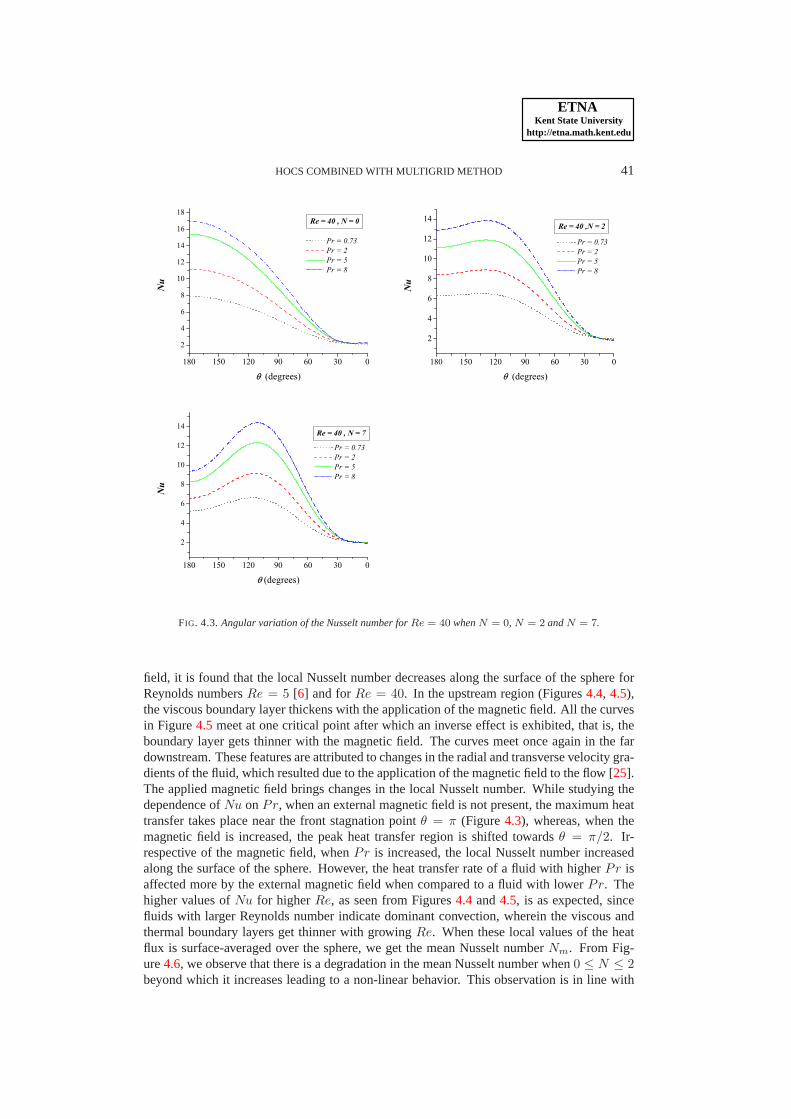
FIG. 4.3.Angular variation of the Nusselt number forRe = 40 whenN = 0, N = 2 andN = 7.

field, it is found that the local Nusselt number decreases along the surface of the sphere forReynolds numbersRe = 5 [6] and forRe = 40. In the upstream region (Figures4.4, 4.5),the viscous boundary layer thickens with the application ofthe magnetic field. All the curvesin Figure4.5 meet at one critical point after which an inverse effect is exhibited, that is, theboundary layer gets thinner with the magnetic field. The curves meet once again in the fardownstream. These features are attributed to changes in theradial and transverse velocity gra-dients of the fluid, which resulted due to the application of the magnetic field to the flow [25].The applied magnetic field brings changes in the local Nusselt number. While studying thedependence ofNu onPr, when an external magnetic field is not present, the maximum heattransfer takes place near the front stagnation pointθ = π (Figure4.3), whereas, when themagnetic field is increased, the peak heat transfer region isshifted towardsθ = π/2. Ir-respective of the magnetic field, whenPr is increased, the local Nusselt number increasedalong the surface of the sphere. However, the heat transfer rate of a fluid with higherPr isaffected more by the external magnetic field when compared toa fluid with lowerPr. Thehigher values ofNu for higherRe, as seen from Figures4.4 and4.5, is as expected, sincefluids with larger Reynolds number indicate dominant convection, wherein the viscous andthermal boundary layers get thinner with growingRe. When these local values of the heatflux is surface-averaged over the sphere, we get the mean Nusselt numberNm. From Fig-ure4.6, we observe that there is a degradation in the mean Nusselt number when0 ≤ N ≤ 2beyond which it increases leading to a non-linear behavior.This observation is in line with




180 150 120 90 60 30 01.8

2.1

2.4

2.7

3.0

3.3

3.6 Re = 5 , Pr = 0.73

Nu

(degrees)

N = 0 N = 0.5 N = 2 N = 8

180 150 120 90 60 30 01

2

3

4

5

6

7

8Re = 5 , Pr = 8

Nu

(degrees)

N = 0 N = 0.5 N = 2 N = 8

FIG. 4.4.Angular variation of the Nusselt number forRe = 5 whenPr = 0.73 andPr = 8.

180 150 120 90 60 30 0

2

3

4

5

6

7

8 Re = 40 , Pr = 0.73

Nu

(degrees)

N = 0 N =0.5 N = 2 N = 8

180 150 120 90 60 30 00

2

4

6

8

10

12

14

16

18Re = 40 , Pr = 8

Nu

(degrees)

N = 0 N = 0.5 N = 2 N = 8

FIG. 4.5.Angular variation of the Nusselt number forRe = 40 whenPr = 0.73 andPr = 8.

the recent experimental findings of Uda et al. [27] and Yokomine et al. [31]. In particular,to compare our results with the recent experimental resultsof Yokomine et al. at low valuesof N up to0.1, simulations are made with KOH solution withPr = 5 for Re = 5 and 40,and the mean Nusselt number is presented in Figure4.7. The degradation of the heat transferfound in this study, at low values ofN , is also in agreement with experimental results [31].The increasedNm with Pr, as observed here, is in agreement with [18] in their study withoutmagnetic field.

5. Conclusions.A higher-order compact scheme is combined with an accelerated multi-grid method in spherical polar coordinates to simulate the steady forced convective heat trans-fer from a sphere under the influence of an external magnetic field. The speedy convergenceof the solution using the multigrid method and accelerated multigrid method is illustrated.The computational efficiency of the higher-order compact scheme over second-order accu-rate scheme is presented. The angular variation of the Nusselt number and mean Nusseltnumber are calculated and compared with recent experimental results. Upon applying themagnetic field, a slight degradation of the heat transfer is found for moderate values of the in-teraction parameterN, and for high values ofN , an increase in the heat transfer is observed,leading to nonlinear behavior.




0 2 4 6 8

2.78

2.79

2.80

2.81

Nm

N

Pr = 0.065

0 2 4 6 84.94

4.96

4.98

5.00

5.02

5.04

5.06

5.08

Nm

N

Pr = 0.73

0 2 4 6 88.60

8.65

8.70

8.75

8.80

8.85

8.90

Nm

N

Pr = 5

0 2 4 6 89.90

9.95

10.00

10.05

10.10

10.15

10.20

10.25

Nm

N

Pr = 8

FIG. 4.6.Variation of the mean Nusselt numberNm with magnetic fieldN for differentPr whenRe = 40.

0.00 0.02 0.04 0.06 0.084.304

4.305

4.306

4.307

4.308

4.309

4.310

8.675

8.680

8.685

8.690

8.695

8.700

Nm

N

Re = 5, Pr = 5

Re = 40, Pr = 5

FIG. 4.7.Mean Nusselt number versus interaction parameter (N < 0.1) for aqueous KOH solution (Pr ≈ 5)whenRe = 5 andRe = 40.




REFERENCES

[1] I. ATLAS AND K. BURRAGE, A high accuracy defect-correction multigrid method for thesteady incompress-ible Navier-Stokes equations, J. Comput. Phys., 114 (1994), pp. 227–233.

[2] L. BARANYI , Computation of unsteady momentum and heat transfer from a fixed circular cylinder in laminarflow, J. Comput. Appl. Mech., 4 (2003), pp. 13–25.

[3] J. H. BOYNTON, Experimental study of an ablating sphere with hydromagnetic effect included, J. Aerosp.Sci., 27 (1960), p. 306.

[4] A. B RANDT AND I. YAVNEH, Accelerated multigrid convergence and high-Reynolds recirculation flows,SIAM J. Sci. Comput., 14 (1993), pp. 607–626.

[5] G. Q. CHEN, Z. GAO, AND Z. F. YANG, A perturbationalh4 exponential finite difference scheme for con-vection diffusion equation, J. Comput. Phys., 104 (1993), pp. 129–139.

[6] S. C. R. DENNIS, J. D. A. WALKER , AND J. D. HUDSON, Heat transfer from a sphere at low Reynoldsnumbers,J. Fluid Mech., 60 (1973), pp. 273–283.

[7] Z. G. FENG AND E. E. MICHAELIDES, A numerical study on the transient heat transfer from a sphere athigh Reynolds and Peclet numbers, Int. J. Heat Mass Trans., 43 (2000), pp. 219–229.

[8] L. FUCHS AND H. S. ZHAO, Solution of three-dimensional viscous incompressible flows by a multigridmethod, Internat. J. Numer. Methods Fluids, 4 (1984), pp. 539–555.

[9] U. GHIA , K. N. GHIA , AND K. N. SHIN, High-Re solutions for incompressible flow using the Navier-Stokesequations and a multigrid method, J. Comput. Phys., 48 (1982), pp. 387–411.

[10] M. M. GUPTA, High accuracy solutions of incompressible Navier-Stokes equations, J. Comput. Phys., 93(1991), pp. 343–359.

[11] M. M. GUPTA, J. KOUATCHOU, AND J. ZHANG, A compact multigrid solver for the convection-diffusionequation, J. Comput. Phys., 132 (1997), pp. 123–129.

[12] , Comparison of second- and fourth-order discretizations for the multigrid Poisson solver, J. Comput.Phys., 132 (1997), pp. 226–232.

[13] S. R. K. IYENGAR AND R. P. MANOHAR, High order difference methods for heat equation in polar cylin-drical coordinates, J. Comput. Phys., 72 (1988), pp. 425–438.

[14] M. K. JAIN , R. K. JAIN , AND M. K RISHNA, A fourth-order difference scheme for quasilinear Poissonequation in polar coordinates, Comm. Numer. Methods Engrg., 10 (1994), pp. 791–797.

[15] G. H. JUNCU AND R. MIHAIL , Numerical solution of the steady incompressible Navier Stokes equations forthe flow past a sphere by a multigrid defect correction technique, Internat. J. Numer. Methods Fluids, 11(1990), pp. 379–395.

[16] J. C. KALITA AND R. K. RAY , A transformation-free HOC scheme for incompressible viscous flows past animpulsively started circular cylinder, J. Comput. Phys., 228 (2009), pp. 5207–5236.

[17] S. KARAA AND J. ZHANG, Convergence and performance of iterative methods for solving variable coefficientconvection-diffusion equation with a fourth-order compact difference scheme, Comput. Math. Appl., 44(2002), pp. 457–479.

[18] V. N. KURDYUMOV AND E. FERNANDEZ, Heat transfer from a circular cylinder at low Reynolds numbers,J. Heat Transfer, 120 (1998), pp. 72–75.

[19] M.-C. LAI , A simple compact fourth-order Poisson solver on polar geometry, J. Comput. Phys., 182 (2002),pp. 337–345.

[20] M. L I , T. TANG, AND B. FORNBERG, A compact fourth-order finite difference scheme for the steady incom-pressible Navier-Stokes equations, Internat. J. Numer. Methods Fluids, 20 (1995), pp. 1137–1151.

[21] A. L. PARDHANANI , W. F. SPOTZ, G. F. CAREY, A stable multigrid strategy for convection-diffusion usinghigh order compact discretization, Electron. Trans. Numer. Anal., 6 (1997), pp. 211–223.http://etna.mcs.kent.edu/vol.6.1997/pp211-223.dir

[22] W. E. RANZ AND W. R. MARSHALL, Evoparation from drops: part I, Chem. Eng. Prog., 48 (1952), pp. 141–146.

[23] , Evoparation from drops: part II, Chem. Eng. Prog., 48 (1952), pp. 173–180.[24] T. V. S. SEKHAR, R. SIVAKUMAR , AND T. V. R. RAVI KUMAR, Incompressible conducting flow in an

applied magnetic field at large interaction parameters, AMRX Appl. Math. Res. Express, 2005 (2005),pp. 229–248.

[25] T. V. S. SEKHAR, R. SIVAKUMAR , T. V. R. RAVI KUMAR , AND K. SUBBARAYUDU , High Reynolds numberincompressible MHD flow under lowRm approximation, Int. J. Nonlin. Mech., 43 (2008), pp. 231–240.

[26] M. C. THOMPSON AND J. H. FERZIGER, An adaptive multigrid technique for the incompressible Navier-Stokes equations, J. Comput. Phys., 82 (1989), pp. 94–121.

[27] N. UDA , A. M IYAZAWA , S. INOUE, N. YAMAOKA , H. HORIIKE, AND K. M IYAZAKI , Forced convec-tion heat transfer and temperature fluctuations of lithium under transverse magnetic fields, J. Nucl. Sci.Technol., 38 (2001), pp. 936–943.

[28] S. P. VANKA , Block-implicit multigrid solution of Navier-Stokes equations in primitive variables, J. Comput.Phys., 65 (1986), pp. 138–158.

http://etna.mcs.kent.edu/vol.6.1997/pp211-223.dir




[29] P. WESSELING, An Introduction to Multigrid Methods,Wiley, Chichester, 1992.[30] S. WHITAKER, Forced convection heat transfer correlations for flow in pipes, past flat plates, single spheres,

and for flow in packed beds and tube bundles, AIChE J., 18 (1972), pp. 361–371.[31] T. YOKOMINE, J. TAKEUCHI , H. NAKAHARAI , S. SATAKE , T. KUNUGI, N. B. MORLEY, M. A. A BDOU,

Experimental investigation of turbulent heat transfer of high Prandtl number fluid flow under strongmagnetic field, Fusion Sci. Technol., 52 (2007), pp. 625–629.

[32] J. ZHANG, Accelerated multigrid high accuracy solution of the convection-diffusion equations with highReynolds number, Numer. Methods Partial Differential Equations, 13 (1997),pp. 77–92.

[33] , Numerical simulation of 2D square driven cavity using fourth-order compact finite differenceschemes, Comput. Math. Appl., 45 (2003), pp. 43–52.

a combined fourth-order compact scheme …etna.mcs.kent.edu/vol.39.2012/pp32-45.dir/pp32-45.pdf ·...

Documents