a common processing and statistical frame for label … · oksana riba grognuz: label-free...
TRANSCRIPT

Oksana Riba Grognuz: Label-Free Quantitative Proteomics i
A Common Processing and Statistical
Frame for Label-Free Quantitative Proteomic Analyses
Master’s Thesis in Proteomics and Bioinformatics
By Oksana Riba Grognuz
President of Jury:
Dr. Jean-Charles Sanchez, Biomedical Proteomics Research Group, University of Geneva
Supervisor:
Dr. Patrice Waridel, Protein Analysis Facility, Center for Integrative Genomics
Co-supervisors:
Dr. Frédéric Schütz, Bioinformatics Core Facility, Swiss Institute of Bioinformatics
Li Long, Vital-IT Group, Swiss Institute of Bioinformatics
Master Program Coordinator:
Dr. Patricia Palagi, Proteome Informatics Group, Swiss Institute of Bioinformatics
Geneva, July 2nd 2009

Oksana Riba Grognuz: Label-Free Quantitative Proteomics ii

Oksana Riba Grognuz: Label-Free Quantitative Proteomics iii
Thesis Statement
The goal of current work is to deliver an integrated bioinformatics pipeline for label-free proteomics that incorporates various available open source quantification programs into a common processing and analytical framework. The intention is to use such common framework to carry out an appropriate performance evaluation of the available software packages, to identify their critical parameters and to validate the workflow using the controlled data set. The validated pipeline will be an open resource for label-free quantification accessible as web deployed application.
The analytical software pipeline should be developed in a flexible way allowing for its extension to include more quantification programs and statistical tools. It should deliver means for software parameter tuning and allow uniting and comparing the results from different programs and different experiences. The data shall be processed in a fully automated way using any of the incorporated open source software packages and the combination of desired statistical methods. The framework shall include tools for data quality assessment and allow for user intervention if necessary.

Oksana Riba Grognuz: Label-Free Quantitative Proteomics iv
Abstract
There is a growing interest towards label-free mass spectrometry based quantification in the field of proteomics. Following the advances in mass spectrometer technology, new techniques for data analysis evolve and new tools for quantification are being developed. The abundance of the available open source algorithmic approaches, the differences in the pre- and post- processing of data, make it difficult to select an appropriate tool for label-free quantitative analysis. Moreover it is a hard task to parameterise the selected tool to achieve its optimal performance within a given analytical platform.
Responding to the need for adequate performance evaluation of reported software, the proposed analytical platform provides a common processing and statistical framework for label-free proteomic analyses with different open-source programs for TIC-based label-free quantification. The flexible structure of the pipeline is extensible to include more common processing and analytical options and to integrate additional software packages. The latter one requires the development of a dedicated converter of the extracted list of matched features to a common input format for the analytical workflow.
Currently pipeline includes two quantification programs: SpecArray and SuperHirn. Critical performance parameters are determined for each integrated software package based on the receiver operating characteristic (ROC) analysis and result trueness and precision. The analyses are carried on the controlled data set that contains standard proteins at known concentrations. The optimal parameter settings are suggested for LTQ-Orbitrap based analytical platform. The pipeline is then validated with biological data using the determined optimal settings.

Oksana Riba Grognuz: Label-Free Quantitative Proteomics v
Abbreviations
AUC – Area under the curve
CV – Coefficient of Variation
FN – False Negative
FP – False Positive
LC – Liquid Chromatography
LF – Label Free
LPE – Local Pooled Error
MS – Mass Spectrometry
PPM - Parts Per Million
SA – SpecArray
SAM – Significance Analysis for Microarrays
SD – Standard Deviation
SH - SuperHirn
TIC – Total Ion Current
TN – True Negative
TP – True Positive

Oksana Riba Grognuz: Label-Free Quantitative Proteomics vi
Table of Contents I. Introduction............................................................................................... 1
II. Theoretical Framework ................................................................................ 3
A. Mass spectrometers ...........................................................................3
1. High resolution mass spectrometers .................................................3
2. Hybrid mass spectrometer: LTQ-Orbitrap ..........................................3
B. Label-free quantification approaches ....................................................4
1. Spectral counting ...........................................................................4
2. TIC-based quantification .................................................................4
C. TIC-based quantification algorithms .....................................................5
1. Data processing .............................................................................5
2. Open source software .....................................................................8
D. Differential Expression Analysis ......................................................... 10
1. Choice of statistical method........................................................... 10
2. Statistical methods....................................................................... 12
3. Significance threshold................................................................... 14
III. Materials and Methods................................................................................15
A. Data sets ........................................................................................ 15
1. Test data set ............................................................................... 15
2. Biological data set ........................................................................ 16
3. Data quality assessment ............................................................... 16
B. Framework development................................................................... 16
1. Framework scope......................................................................... 17
2. Data structure ............................................................................. 17
3. Input and output.......................................................................... 18
4. Accuracy scoring.......................................................................... 18
C. Parameter tuning............................................................................. 19
IV. Validation Method ......................................................................................21
A. Accuracy in terms of specificity and sensitivity..................................... 21
B. Accuracy in terms of precision and trueness ........................................ 22
V. Results.....................................................................................................24
A. Software Parameterisation ................................................................ 24
1. SpecArray ................................................................................... 25
2. SuperHirn ................................................................................... 28
B. Biological data analysis..................................................................... 31
VI. Discussion ................................................................................................35
A. Adjusting SpecArray scores ............................................................... 35
B. SuperHirn redundant extraction ......................................................... 36

Oksana Riba Grognuz: Label-Free Quantitative Proteomics vii
C. Conflicting peptide ratios .................................................................. 37
D. Thresholds to infer differential expression ........................................... 39
E. Grouping peptides to proteins............................................................ 41
VII. Conclusions ..............................................................................................42
VIII. References................................................................................................44
IX. Appendix ..................................................................................................47
A. Test data set quality control .............................................................. 47
B. Validation of accuracy ranking ........................................................... 49
C. SpecArray parameter tuning.............................................................. 50
D. SuperHirn parameter tuning.............................................................. 51
List of Figures Figure 1: Target processing and statistical analysis pipeline
Figure 2: Feature extraction and matching
Figure 3: Intensity integration
Figure 4: Precision and trueness
Figure 6: Validation of accuracy scoring: sub-scores for trueness and precision measures of validation data set
Figure 5: Effect of SD sub-score weight on scoring performance
Figure 7: Framework overview
Figure 8: Types of tested parameters based on intensity, mass-to-charge ratio and retention time
Figure 9: SpecArray accuracy sub-scores for different parameter settings (Table 15)
Figure 10: SpecArray ROC sub-scores for different parameter settings (Table 15): A) T-test P-value classifier, B) Fold change classifier
Figure 11: Feature ratio measurement in linear and exponential series by SpecArray with optimal parameter settings (test 19, Table 15)
Figure 12: Sample 2 versus sample 1 feature fold change using different parameter settings of SpecArray: A) default parameters (test 1, Table 15), B) optimal parameters (test 19, Table 15)
Figure 13: SuperHirn accuracy sub-scores for different parameter settings (Table 16)
Figure 14: SuperHirn ROC sub-scores for different parameter settings (Table 16): A) T-test P-value classifier, B) Fold change classifier
Figure 15: SuperHirn Exponential and Linear Series: good examples of feature ratio measurements using optimal parameter settings (test 37, Table 16)
Figure 16: SuperHirn Exponential and Linear Series: bad examples of feature ratio measurements using optimal parameter settings (test 37, Table 16)
Figure 17: Sample 2 versus sample 1 feature fold change using different parameter settings of SuperHirn: A) default parameters (test 10, Table 16), B) optimal parameters (test 37, Table 16)
Figure 18: Features extracted from biological data set, sample 2 (40°C) / sample 1 (37 °C), using A) SpecArray, B) SuperHirn

Oksana Riba Grognuz: Label-Free Quantitative Proteomics viii
Figure 19: Protein identification overlap between SpecArray and SuperHirn
Figure 20: Few differentiated peptides in default SpecArray results can yield maximal ROC measures
Figure 21: Example of redundantly extracted peptide
Figure 22: A) Conflicting albumin ratios in SuperHirn results for the test data, B) MS/MS spectrum for feature 1
Figure 23: MS/MS spectrum of A) feature 2 B) feature 3 ( 22 A)
Figure 24: Ratios of peptides between two test samples assigned differential expression by applying a threshold on t-test p-value of SpecArray (A) and SuperHirn (B) results and by applying a fold change
Figure 25: Problem using t-test: low p-values for small fold change (A) and high p-values for big fold change (B)
Figure 26: Dendrogram of all test data set features extracted with SpecArray using default parameters, test 1 (Table 15)
Figure 27: Dendrogram of spiked proteins from test data set extracted with SpecArray using default parameters, test 1 (Table 15)
Figure 28: Dendrogram of all test data set features extracted with SuperHirn using default parameters, test 10 (Table 16)
Figure 29: Dendrogram of spiked proteins from test data set extracted with SuperHirn using default parameters, test 10 (Table 16)
List of Tables Table 1: SpecArray Tools ................................................................................... 9
Table 2: SpecArray and SuperHirn processing....................................................... 9
Table 3: T-test variations ................................................................................. 12
Table 4: Spiked protein ratios in E.coli lysate (test data set)................................. 15
Table 5: Mascot search parameters ................................................................... 15
Table 6: Statistical parameters for software tuning.............................................. 19
Table 7: Biological data extraction..................................................................... 31
Table 8: Protein differential expression assignment overlap in sample 2 (40°C) / sample 1 (37°C) between SpecArray and SuperHirn ............................................ 32
Table 9: SuperHirn redundant extraction of feature assigned to HSP71_HUMAN..... 34
Table 10: Effect of SpecArray score adjustment based on the number of extracted features ......................................................................................................... 36
Table 11: The effect of MISD and intensity threshold on redundant feature extraction.................................................................................................................... 37
Table 12: Three peptides assigned to albumin with comflicting ratios (Figure 22 A) . 39
Table 13: Data sets used for accuracy ranking validation ..................................... 49
Table 14: Test data accuracy scores .................................................................. 49
Table 15: SpecArray parameter testing.............................................................. 50
Table 16: SuperHirn parameter testing .............................................................. 51

Oksana Riba Grognuz: Label-Free Quantitative Proteomics 1
I. Introduction Mass spectrometry (MS) based proteomics in combination with bioinformatics tools plays an important role in the analysis of biological data sets. A core MS-based method is to use an integrated liquid chromatography mass spectrometry (LC-MS) system, especially suitable for the analysis of complex protein mixtures. Although MS analysis is inherently qualitative, the state of art LC-MS technology is capable of extracting quantitative information on changes in protein abundance (Ackermann et al).
The numerous reported strategies to derive quantitative information from MS analyses can be divided into labelled and label-free approaches. The stable isotope labelling strategies were first to emerge in the field of proteomics (Turck et al). Although these labelling strategies are successfully used for relative quantification of proteomic data, their use is limited to the direct comparison of up to eight experiments, due to the restricted availability of labelling reagents. Additional limitations of labelled techniques relate to their relatively high cost and time required for sample labelling (Kühner et al, Vandenbogaert et al).
The label-free approaches represent an alternative strategy of lower complexity and cost without the limitation in the number of compared samples. Free from the requirement of sample mixing, the analyses can include data sets obtained at different time or place (Ackermann et al, Vandenbogaert et al). Furthermore, there is evidence that label-free techniques yield wider dynamic range and higher proteome coverage (Bantscheff et al). The investigation of quantitative properties can be done at two levels: using the total ion current (TIC) at MS1 detection level or using MS/MS selection frequency. This work focuses on MS1 level quantification that is in general more sensitive and accurate than MS/MS spectral counting. In addition, TIC-based quantification tackles the problem of insufficient sampling of low-abundance components associated with tandem mass spectrometry in data dependent acquisition mode. Virtually any feature detected by mass spectrometer can be quantified through relevant ion current integration (America and Cordewener, Kühner et al).
On one hand, recent advances in MS technology have induced substantial quality improvement of the label-free techniques. On the other hand, the complexity of high-dimensional LC-MS data raises a challenge of developing a set of advanced bioinformatics solutions to carry out computational and statistical tasks (Wong, J. W. H. et al). Open-source software packages emerging in label-free proteomics field target further improvement of the reliability and accuracy of final results. However, although a wide number of algorithms were reported, the adequate assessment of their performance is complicated by differences in input/output formats, functionality, user interfaces and parameter tuning options.
The available tools were optimised for specific types of mass analysers and differ in the level of output complexity starting from a simple list of features with quantitative and statistical values up to sophisticated expression profile analyses. A particular attention should be given to software parametrisation required to achieve maximum efficiency on a given analytical platform. Even within the same analytical platform, changes in parameter settings may lead to considerable differences in final result quality. Software parametrisation requires a thorough understanding of program operation and often demands extended informatics competencies. Thus restricted availability of informatics resources within a laboratory may limit the use of software tools (Deutsch et al).
A number of previous works evaluate the performance of different software solutions both commercial and open source (America and Cordewener, Mueller 2008 et al, Wong J.W.H. et al). However the performance of available open source programs was never fully integrated within a common analytical framework for adequate comparison using the same test data set. Lange (2008) and colleagues assessed performance of alignment algorithms of several open source programs. Suggested evaluation procedure is based on the alignment of two benchmark data sets containing already

Oksana Riba Grognuz: Label-Free Quantitative Proteomics 2
Figure 1: Target processing and statistical analysis pipeline
extracted peptide signals. Recently developed open source framework Corra integrates existing tools for feature extraction and alignment into an APML-based environment (Brusniak et al). Although Corra allows for comprehensive differential expression analysis within a common frame, it does not provide any tools for performance evaluation.
Responding to the need for adequate performance evaluation of reported software, the goal of current work is to develop a bioinformatics pipeline readily extensible for integration of a software package of interest into a common processing and statistical framework. The target pipeline should process the MS data input with different quantitative programs in order to achieve an equivalent quantitative output converted to a common format used as input for common analysis (Figure 1). The input files should be automatically processed into a set of tables, figures and data objects containing such information as differential expression profiles, clustering, type I and II error analysis, etc. Combining several software suits within the same framework will facilitate the task of inter-software evaluation by making the performance more appraisable. Supplemented with the appropriate analytical tools the framework will be used to identify critical performance parameters for each software program. In addition, the reliability of quantitative measures can be improved by unifying and comparing the results of different tools (Mueller 2008 et al, Lange 2008 et al).

Oksana Riba Grognuz: Label-Free Quantitative Proteomics 3
II. Theoretical Framework
A. Mass spectrometers The performance of the mass spectrometer is central to the quality of results obtained with label-free quantification. A high-resolution mass spectrometer is required to ensure optimum feature extraction from MS1 level, whereas, a sensitive mass spectrometer with high MS/MS sampling rate suits best for MS2 detection.
1. High resolution mass spectrometers
The resolution of the mass spectrometer is a critical attribute of label-free quantitative approaches based on TIC. Higher resolution improves the identification of charge state and isotopic pattern assignment to overlapping peaks. Furthermore, the reliability of resulting expression profiles is improved by minimising the influence of interfering signals of similar masses that can be mapped at narrower mass-to-charge ratio intervals (America and Cordewener, Bantscheff et al, Marshall and Hendrickson).
The advances in mass analyser technology and development of new MS-based experimental approaches permitted the use of high-resolution mass spectrometers in the field of proteomics (Aebersold and Mann, Marshall and Hendrickson). Two types of analysers are compatible with liquid chromatography and atmospheric ionisation sources used for proteomic analyses: Fourier transform (FT) instruments and reflectron time-of-flight (TOF) (Marshall and Hendrickson).
a. Fourier transform (FT) instruments
FT mass analysers, ion cyclotron resonance (ICR) and Orbitrap are trapping instruments that detect ions as time domain signals converted to frequency domain by Fourier transformation. In ICR mass spectrometer ions orbit in the magnetic field at a frequency characteristic of their mass-to-charge ratio value. Ion image charge is detected by exciting ions to a larger radius with a pulse of radio frequency energy. Orbitrap is a trapping device that can be operated as a mass analyser, where ions orbit along the axis of electrostatic field created between an outer barrel-like electrode and a coaxial inner spindle-like electrode at a frequency inversely proportional to the square root of mass-to-charge ratio. Orbitrap detects an image current of ions excited to a larger orbit (Murray et al).
The benefits of FT-MS are high sensitivity, mass accuracy, resolution and dynamic range. The disadvantage is low peptide-fragmentation efficiency. The Orbitrap has lower mass resolution and mass accuracy in comparison to ICR, but has higher sensitivity and mass-to-charge ratio range when ions are injected from an external source. FT mass analysers are optimal for ions of mass-to-charge ratio smaller than 5000 (Marshall and Hendrickson).
b. TOF instruments
TOF instruments are based on the measurement of transit time of ions accelerated by a pulsed direct-current electric field and flying in high vacuum in the absence of external electrical or magnetic fields (Marshall and Hendrickson). TOF instruments have high mass accuracy, resolution, sensitivity and speed. These instruments have in principle no upper mass-to-charge ratio limit and are advantageous for applications that require fast acquisition of more than one spectrum per second (Marshall and Hendrickson).
2. Hybrid mass spectrometer: LTQ-Orbitrap
A hybrid LTQ-Orbitrap mass spectrometer combines a linear ion trap with radial ejection and an Orbitrap mass analyzer (Makarov et al). This instrument supplements the accurate mass capability of Orbitrap with sensitivity and high MS/MS sampling

Oksana Riba Grognuz: Label-Free Quantitative Proteomics 4
rate of a linear ion trap. Extensive MS/MS sampling improves the performance of spectral counting approaches and TIC-based approaches that rely on parallel or alternate full survey MS detection and MS2 identification (America and Cordewener, Old et al, Fu et al, Xia et al).
B. Label-free quantification approaches The two main strategies for label-free quantification are spectral counting and TIC-based approach. The first one estimates relative protein abundance based on the number of relevant peptide fragment MS/MS spectra. The second relies on the comparison of chromatographic peak intensities across multiple consecutive LC-MS runs. Spectral counting methods tend to be less accurate and have smaller dynamic range than TIC-based approaches (America and Cordewener, Wang M. et al, Mueller 2008 et al, Bantscheff et al). The performance of spectral counting can be improved using sensitive mass analyser with high MS/MS sampling rate, such as linear ion trap (Old et al). On the other side, a substantial improvement in the accuracy of quantification by ion intensities can be achieved using high resolution and high accuracy mass analysers, such as Fourier transform (FT) analysers.
1. Spectral counting
The spectral counting approach emerged from the empirical observation of higher frequency of selection of a particular protein for MS/MS analysis if more of that protein was present in a sample. The quantitative dimension is established through the comparison of normalised count of peptide identifications for a given protein. This approach relies on MS/MS information for both identification and quantification and therefore requires high MS/MS sampling rate for optimal performance (America and Cordewener, Bantscheff et al). The main advantage of spectral counting is the conceptual simplicity of simultaneous identification and quantification through extensive MS/MS sampling. On the other hand the reliability of final results strongly depends on peptide identification (Wang M. et al). In addition, the quality of inferred protein abundance depends on software and parameters used for MS/MS acquisition as well as on post-processing of spectral counts (Choi et al, Fu et al, Zhang B et al, Xia et al). Within the scope of current wok the spectral counting approach is not considered in further detail.
2. TIC-based quantification
TIC-based approach relies on the observation of proportionality between peptide concentration and peak volume detected in LC-MS analysis (America and Cordewener). The differences in expression level are measured by comparing the mass spectrometric signal intensity of corresponding precursor ions across LC-MS runs, given that the measurements are performed under identical conditions. The ion chromatograms for every potential peptide are extracted from LC-MS scan and then the spectrometric peak volume is integrated over the chromatographic retention time scale (Bantscheff et al, Kühner et al). Since peptide quantification is uncoupled from identification, an MS/MS analysis is required to confirm peptide identities.
To meet the assumption of identical conditions for different LC-MS runs, the method requires highly reproducible HPLC separation procedure. The stability of elution ensures high peak capacity in retention time dimension. The capacity in mass-to-charge ratio dimension requires a sufficient resolution of the full scan MS spectra (America and Cordewener). Survey scan sampling rate optimisation can be achieved by separating MS and MS/MS analyses. High frequency full scan MS analysis is used to estimate the abundance values and generate the inclusion list with differentiated features for the subsequent MS/MS identification analysis. Although this approach benefits from selective MS/MS identification of peptides of interest, the data analysis may become more complicated.

Oksana Riba Grognuz: Label-Free Quantitative Proteomics 5
m/z
Retention time
m/z
Retention timeInte
nsity
1. feature detection in each LC-MS run2. quantification: intensity integration3. creation of 2D feature map4. matching and alignment across LC-MS runs
m/z
Retention timeInte
nsity
m/z
Retention time
m/z
Retention time
Retention timeInte
nsity
1.
2. 2.
3.3.
4.
Figure 2: Feature extraction and matching
An alternative approach is to collect MS1 intensities and identification information in a single LC-MS run. This can be done either by simultaneous performance of acquisition and fragmentation scans or by switching between MS and MS/MS modes (America and Cordewener, Bantscheff et al). The main disadvantage of simultaneous acquisition is relative uncertainty regarding the true precursor ion (Niggeweg et al). The alternate scanning approach reduces the sampling rate of intact peptide signals. However if the right balance between scanning frequency of MS and MS/MS modes is found, this approach benefits from the limited amount of MS/MS information that can be used as a landmark in the alignment procedure (America and Cordewener, Wong, J. W. H. et al).
C. TIC-based quantification algorithms
1. Data processing
Main steps in quantitative TIC-based LC-MS data processing are the following (America and Cordewener, Lange 2008 et al, Tautenhahn et al):
• Preprocessing
• Feature extraction (Figure 2, steps 1 - 3)
• Matching and alignment (Figure 2, step 4)
• Normalisation
• Statistical analysis
Each LC-MS run generates a complex high-dimensional data set. The goal is to discern from a multitude of detected signals, the peaks that correspond to peptides and to extract the abundance information. Peptide peaks are detected through their characteristic isotope pattern (Figure 2, step 1). The measure of abundance for a particular peptide stems from the intensity levels over the elution time for its mono-isotopic mass ion, or for several isotopes (Figure 2, step 2).
The recognised peptide peaks are extracted to features mapped in the dimensions of retention time and mass-to-charge ratio (Figure 2, step 3). Features are defined at least by a particular charge state, retention time, monoisotopic mass-to-charge ratio and integrated intensity volume. Optional characteristics may include isotope distribution, molecular weight and other information. Thus the continuous data set from each LC-MS run is converted to a list of discrete features with specific time and mass coordinates. The features extracted in each run are matched according to their time and mass coordinates and charge state to corresponding features in the other runs (Figure 2, step 4). Feature matching requires the alignment in retention time and to smaller extent in mass to charge dimension, because of technical and experimental variations inherent to LC-MS data. The result of the alignment and matching

Oksana Riba Grognuz: Label-Free Quantitative Proteomics 6
procedure is a consensus map that contains features whose characteristics include the intensity volume information for each LC-MS run.
A common output of available quantification programs is a data structure, often a table or an array, with the aligned features. Such feature lists may include MS/MS identification information and related scores or probabilities. The reported abundance measures as well as the retention time and mass may be subject to normalisation discussed in section II.C.1.d. In addition to the above mentioned output, the programs provide means for comprehensive statistical analysis of differential expression. However in the scope of current work such options are not considered.
a. Preprocessing
Goal: reduce noise and enhance signal
The spectra obtained with LC-MS experiments contain a mixture of peptide signals and different types of noise, such as electronic and chemical noise. Noise suppression and baseline correction can be accomplished prior to quantification procedure either by subtracting an additive baseline model or using noise filtering to smooth and enhance the MS signal. Digital noise filters include wavelet transform, Savitzky-Golay, loess, moving average and other filters (America et al, Listgarten and Emili).
On the contrary, noise filtering may complicate isotope pattern assignment by filtering out the least intense isotopes. The remaining isotopes may not be sufficient for pattern fitting, especially if the minimum number of isotopes is specified. Furthermore, denoising removes the chemical component of the noise that may indicate the consistency of measurements and ionisation performance and therefore be used to correct errors in spectra.
Another commonly used method for raw profile data reduction is peak centroiding. Peaks are approximated to their centroids according to the specified range, often set at mass-to-charge ratio values of half-peak height.
b. Feature extraction
Goal: transform raw or preprocessed LC-MS data into a list of features
Feature extraction is a crucial step in data processing, since all subsequent analysis is based on the information extracted in this step. The algorithm should identify maximum number of true features and integrate relevant abundance values, while keeping low false positive detection. Features are characterised by the relevant monoisotopic mass, retention time, charge state, abundance and other parameters. The main challenges stem from the presence of overlapping isotope patterns, multiple charge states, low intensity features of interest, chemical and instrument noise, varying ionisation efficiencies, deviation from linearity in detector response and limited reproducibility (America and Cordewener, Tautenhahn et al, Noy and Fasulo, Renard et al). A particular concern should be given to tailing peaks that may be erroneously detected as multiple consecutive peaks (America and Cordewener).
If one LC-MS run data is represented as a two-dimensional image, where the horizontal axis is a retention time, the vertical axis is a mass-to-charge ratio and the grey colour level indicates the intensity value (Figure 2, step 1), then feature extraction can be described as a task of determining boundaries and intensities of two-dimensional peptide signals (Tautenhahn et al). Peptide signals are identified through their characteristic isotope distribution by fitting the observed spectral pattern to theoretical isotope distribution models. Additional processing steps are required to handle the overlapping features (Noy and Fasulo, Renard et al). The accuracy and correctness of peptide signal recognition depends on similarity measure used in the comparison of theoretical and observed shapes, on goodness of calculated theoretical model shape and fitting optimisation algorithm.
Peptide peak detection provides the information on monoisotopic mass-to-charge value and peptide charge state. The abundance values of the identified peptide

Oksana Riba Grognuz: Label-Free Quantitative Proteomics 7
m/z
Retention timeInte
nsity
Intensity integration of first 3 isotopes (left) andonly monoisotopic ion (right)
m/z
Retention timeInte
nsity
Figure 3: Intensity integration
signals are estimated based on the intensity of relevant monoisotopic ion or sum of intensities of all or several isotopes (Figure 3). The peak volume of the relevant ion current gives a value of peptide abundance in a given sample (America and Cordewener, Tautenhahn et al).
Quantification approaches relying on monoisotopic mass intensity integration may be
less sensitive especially for larger peptides for which the monoisotopic ion current constitutes a relatively small part of the total signal intensity. On the other side, the summed volume of all isotopes allows for higher sensitivity and accuracy at the cost of increased computational complexity, especially in the case of overlapping isotope patterns (Bantscheff et al, Du et al).
Additional challenge for feature extraction is its computational complexity. A number of approaches emerged to reduce the computation time required for feature extraction starting from the use of batch processing (America and Cordewener) up to data transforms. One of the widely used approaches is binning that transforms LC-MS data into a matrix with the dimensions of mass-to-charge, retention time and intensity. Such transformation divides the mass-to-charge axis on bins of specified width depending on the resolution of mass spectrometer. Finding optimal bin size is crucial for the reliability of this processing method. Too small or too big size may induce data loss because of deteriorated chromatographic shape and increased chromatographic noise level respectively. Alternative approaches include Kalman tracking based, Wavelet based and density based techniques, as well as the combinatory approaches (Aberg et al, America and Cordewener, Listgarten and Emili, Tautenhahn et al).
c. Matching and alignment
Goal: find corresponding features across maps
The comparison of multiple LC-MS runs relies on matching of corresponding features of same charge state in retention time and mass-to-charge ratio dimensions (Figure 2, step 4). Since time and mass information are subject to technical variations, the matching requires feature alignment across LC-MS runs in both dimensions. The main challenges to alignment are posed by the inequality of drift magnitude, the overlapping features and the absence of corresponding features. The observed drifts and distortions are particularly significant in retention time dimension attributable to limited reproducibility and stability of chromatographic system, whereas the mass-to-charge ratio variation caused by instrument noise is of smaller scale (America and Cordewener, Lange 2008 et al, Wang P. et al).
The global alignment of retention time can be done on raw data level by selecting a template file and warping the retention time coordinates of other files to achieve maximum similarity in retention time dimension. However relying only on time coordinates is not sufficient to correct for differing retention time shifts and changes in elution order across runs. Instead of using the raw data, a number of algorithms align the extracted features allowing for local correction of each distinct feature drifts. The alignment of extracted features provides greater flexibility, but is vulnerable to the inaccuracy of feature extraction and fails to account for raw spectra information, such as isotope distribution. A particular concern relates to peptides that exhibit peak tailing and can be therefore detected as multiple features (America and Cordewener, Wang P. et al).

Oksana Riba Grognuz: Label-Free Quantitative Proteomics 8
Multiple data sets of extracted features can be aligned simultaneously (multiple alignment) or sequentially. The latter approach relies on the choice of a template and may lead to unpredictable errors (Wang P. et al). The reported algorithms include such approaches as data binning, multi-scale wavelet decomposition, Hidden Markov Model, clustering and other (America and Cordewener). Pioneer software, SpecArray, solves the alignment problems by allowing for variation in mass-to-charge ratio and retention time of individual features (Li et al). The maximum mass-to-charge variation is set by a threshold, whereas retention time variation is selected according to the smallest possible distance to the calibration curve (section II.C.2.).
An alternative approach is to combine the alignment on raw data level and extracted features level. For example, SuperHirn program relies on a multi-step alignment procedure, where based on raw data clustering the most similar extracted feature data are aligned to each other first. Another approach combines raw spectra and extracted feature information for simultaneous multiple alignment (Wang P. et al). In addition, the available MS/MS identifications can be used as a landmark in the alignment process (America and Cordewener).
d. Normalisation
Goal: correct global errors and technical bias
In order to find the true differences in the abundance it is crucial to account for known sources of systematic biases (Oberg and Vitek). The goal of normalisation procedures is to correct for systematic biases in retention time, mass-to-charge ratio or integrated peptide intensity. The time and mass normalisation corrects global errors and improves feature matching and comparison. Depending on the implemented algorithm retention time and mass normalisation may occur during the alignment procedure. The most essential for results quality is the normalisation of intensity. Intensity normalisation corrects for technical bias introduced during the data measurement, such as carry-over and drifts in ionisation and detector efficiencies (America and Cordewener). The intensity can be normalised prior to feature extraction to improve the comparability across LC-MS runs. This step is particularly important if different experiences are compared. Otherwise intensity normalisation can be applied to estimated feature abundance.
The normalisation can occur on local and global level. Thus given the assumption that overall abundance of all features is equal across samples and their replicate measures, a normalisation can be done by multiplicative correction factor. Other global normalisation approaches rely on distribution parameters of all or part of detected features in the data set. Local normalisation approaches often rely on regression algorithms, such as loess. America and Cordewener discuss the importance of and the advances in different level normalisation, Listgarten and Emili provide for a technical overview of techniques.
e. Statistical analysis, profiling
Goal: infer biologically meaningful information
The statistical analysis of proteomic data is discussed in section II.D.
2. Open source software
Numerous available software packages are available in the filed of label-free quantification and more packages are being developed. Different open source and commercial solutions emerge following the advances of MS technology and cover a wide range of analytical platforms. Mueller (2008) and America and Cordewener review the available software for label-free proteomics. The available software packages implement different algorithms and vary in processing flows for data treatment steps discussed in section II.C.1. Most of open source solutions operate in Linux environment and use mzXML input format for MS data.
Oksana Riba Grognuz: Label-Free Quantitative Proteomics 9
a. Two software generations: SpecArray and SuperHirn
SpecArray algorithm
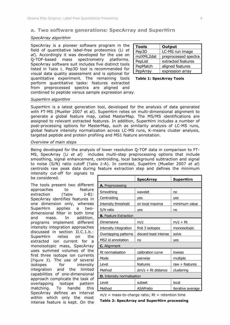
SpecArray is a pioneer software program in the field of quantitative label-free proteomics (Li et al). Accordingly it was developed for the use on Q-TOF-based mass spectrometry platforms. SpecArray software suit includes five distinct tools listed in Table 1. Pep3D tool is recommended for visual data quality assessment and is optional for quantitative experiment. The remaining tools perform quantitative tasks: features extracted from preprocessed spectra are aligned and combined to peptide versus sample expression array.
SuperHirn algorithm
SuperHirn is a latest generation tool, developed for the analysis of data generated with FT-MS (Mueller 2007 et al). SuperHirn relies on multi-dimensional alignment to generate a global feature map, called MasterMap. The MS/MS identifications are assigned to relevant extracted features. In addition, SuperHirn includes a number of post-processing options for MasterMap, such as similarity analysis of LC-MS runs, global feature intensity normalization across LC-MS runs, K-means cluster analysis, targeted peptide and protein profiling and MS1 feature annotation.
Overview of main steps
Being developed for the analysis of lower resolution Q-TOF data in comparison to FT-MS, SpecArray (Li et al) includes multi-step preprocessing options that include smoothing, signal enhancement, centroiding, local background subtraction and signal to noise (S/N) ratio cutoff (Table 2-A). In contrast, SupeHirn (Mueller 2007 et al) centroids raw peak data during feature extraction step and defines the minimum intensity cut-off for signals to be considered.
The tools present two different approaches to feature extraction (Table 2-B): SpecArray identifies features in one dimension only, whereas SuperHirn applies a two-dimensional filter in both time and mass. In addition, programs implement different intensity integration approaches discussed in section II.C.1.b.: SuperHirn relies on the extracted ion current for a monoisotopic mass, SpecArray uses summed volumes of the first three isotope ion currents (Figure 3). The use of several isotopes for intensity integration and the limited capabilities of one-dimensional approach complicate the task of overlapping isotope pattern matching. To handle this SpecArray defines an interval within which only the most intense feature is kept. On the
Tools Output
Pep3D LC-MS run image mzXML2dat preprocessed spectra PepList extracted features PepMatch aligned features PepArray expression array
Table 1: SpecArray Tools
SpecArray SuperHirn
A. Preprocessing
Smoothing wavelet no
Centroiding yes yes
Intensity threshold on local maxima minimum value
S/N ratio yes no
B. Feature Extraction
Dimensions m/z m/z + Rt
Intensity integration first 3 isotopes monoisotopic
Overlapping patterns discard least intense solve
MS2 id annotation no yes
C. Alignment
Rt normalisation calibration curve lowess
Mode pairwise multiple
Level features raw + features
Method ∆m/z + Rt distance clustering
D. Intensity normalisation
Level subset local
Method ASAPratio iterative average
m/z = mass-to-charge ratio; Rt = retention time
Table 2: SpecArray and SuperHirn processing
Oksana Riba Grognuz: Label-Free Quantitative Proteomics 10
contrary, SuperHirn applies a specific procedure to resolve the overlapping patterns and integrate the intensity based on the fitted model.
A major difference in the use of SuperHirn and SpecArray is the integration of MS2 identifications. SpecArray relies exclusively on MS1 level information and any peptide identifications should be carried out in separate MS/MS analyses using the inclusion lists. SuperHirn was developed for LC-MS/MS analyses; it annotates the extracted features with available MS/MS identification (Table 2-B) and transfers these identifications to the matched features. The issues regarding the resolution of MS1 spectra obtained with these approaches are discussed in section II.B.2.
In terms of feature matching and alignment (Table 2-C), SpecArray implements computationally expensive pairwise alignment in contrast to SuperHirn that uses multiple alignment procedure. Pairwise alignment limits the number of feature maps that can be processed with SpecArray (Lange). SpecArray aligns the extracted features by defining a maximum mass-to-charge difference and calculating the distances to retention time calibration curve (RTCC) between each two LC-MS runs. The RTCC is calculated iteratively, removing the low-scoring peptides until only unique pairs remain. All pairwise alignments are then combined to the final consensus map. SuperHirn program relies on a multi-step alignment procedure. First the alignment topology is constructed based on the similarity between raw profile data. Then the multiple alignment of features takes place according to the order defined by the alignment topology and the aligned features are combined into a consensus map. The retention time is normalised during LC-MS alignment using Lowess algorithm.
For intensity normalisation, SpecArray implements ASAPratio tool on subset level, whereas SuperHirn performs local normalisation using an iterative average (Table 2-D).
D. Differential Expression Analysis The major goal of quantitative studies is to determine biologically significant differences in detected feature expression levels. The variability in proteomic data does not only reflect true biological changes in abundance, but also originates from different sources of random variation, such as random effects from biological samples and replicates, and technical measurement variation. The features likely to be differentially expressed must have sufficient level of evidence for biologically relevant change. The selection of such features is done through the following steps (Smyth and Yang):
• Estimating the level of evidence for differential expression for each feature
• Ranking all features by evidence for differential expression
• Choosing threshold to assign significance to changes
1. Choice of statistical method
This work focuses on the application of statistical analysis to estimate the evidence for differential expression and does not consider other approaches such as machine learning. Existing statistical methods can serve as a means to evaluate whether a given variation is likely to be a random fluctuation or a statistically significant change. The choice of statistical method to rank features depends on the number of replicates available, on sample size and on the assumptions that can be made about data.
a. Replicates and sample size
The change in the abundance level for a given feature can be estimated from differences between its distributions in different samples. For example by considering central tendency parameter of replicated values, such as mean or median. Statistical significance of a given change can be inferred from pattern of variation in relevant replicate values. The performance of statistical tests based on distributional

Oksana Riba Grognuz: Label-Free Quantitative Proteomics 11
differences, therefore, depends on the number of replicates. The higher the number of replicates, the higher the confidence of statistical significance assignment and the reliability of inferred conclusions (Oberg and Vitek).
Despite the advantages of using multiple sample replicates, this is not always possible due to the limited amount of sample material or limited MS analysis time (Choi et al, Li and Roxas). In this case nonparametric tests can be applied to estimate the evidence for differential expression. The accuracy of conclusions inferred with nonparametric tests strongly depends on the sample size: the larger, the better. Unfortunately in proteomic experiences limited sample size often leads to insufficient power of nonparametric tests. Therefore, although the number of replicates is not a prerequisite, the accuracy of results can be improved by pooling the replicated samples to form a bigger data set (Batscheff et al). A possible alternative to address the limited replication is to use combined approaches that include both parametric and nonparametric tests for evidence estimates (Li and Roxas).
b. Distributional assumptions and data transformations
Parametric statistical tests, such as the t-test, have higher statistical power than the nonparametric tests, such as permutation tests, if their underlying distributional assumptions are at least approximately met. The most common assumptions are distribution normality and variance stability. The nonparametric tests are free from the assumptions on data distribution, but rely on the assumption of random sampling. The data sets are considered as random samples from underlying populations (Oberg and Vitek).
As distributional assumptions are generally not met by proteomic data, a particular concern should be given to data transformations. In many cases simple logarithmic transformation is enough to approximate the normal distribution. Whereas the distribution of peptide intensity values is strongly right skewed, the distribution of logarithms of intensities will tend to be centralised. The variance is stabilised by converting multiplicative errors into additive effects (Anderle et al, Listgarten and Emili, Oberg and Vitek). For data following a Poisson distribution a square root transformation can be used to stabilise the variance. The optimal variance stabilising transformation of original or log-transformed data can be selected automatically by estimating Box-Cox transformation parameter for a given data set (Nie L. et al 2007, Nie L. et al 2008, America and Cordewener). The parameter value indicates whether the transformation is needed and if needed suggests a type of transformation that suits best, it includes inverse, logarithmic, square root and square transformations.
Transformation and normalization operations may not be enough to achieve data normality and variance stabilization. An alternative approach is to describe the error component of variance using statistical error models (Anderle et al).
c. Challenges in modelling proteomic data
The choice of appropriate statistical method in quantitative proteomic experiences is complicated by challenges in modelling proteomic data structure. The limited amount of sample replicates may impede data modelling with standard distributional assumptions. Small sample sizes result in insufficient power of nonparametric tests. The absence of consistency of observed evidence across samples increases the burden of making inferences on differential expression (Choi et al, Roxas and Li). The above mentioned challenges complicate the application of traditional statistical techniques and require adaptation of statistical techniques developed for microarray analysis to account for specific proteomic data structure (Batscheff et al, Roxas and Li, Li and Roxas).
The assignment of statistical significance to intensity changes can be done at three levels: using sample replicates, using peptide charge states or at protein level using all observed peptides. Whereas sample replicates are of known quantity, protein and peptide level replicates are not known in advance. The number of observed peptide

Oksana Riba Grognuz: Label-Free Quantitative Proteomics 12
charge states and observed peptides per protein is different across proteins and across sample replicates and can only be determined after the measurements were done. Therefore the assessment of significance in protein differences both at peptide and protein levels raises the concern of modelling unequal proteomic data structure (Roxas and Li, Wong J. W. H. et al, Old et al).
Significance testing based on peptide charge states should be avoided. The underlying assumption that peptide charge states are independent protein events is not carefully met due to experimental constraints (Roxas and Li).
2. Statistical methods
The following subsections describe the approaches to measure statistical significance reported in the context of proteomic data analyses. A particular attention is given to microarray methods that were already applied or can be potentially applied in proteomic analyses.
a. Fold Change Ratio
The simplest way to proceed with the selection of differentially expressed features is to rank them by fold change ratio between average sample intensities. The higher the fold change ratio, the higher the evidence for differential expression. The average fold change for sample features on logarithmic scale is calculated as FC = intensityi – intenityj. Unfortunately the use of fold change as a rank test precludes the assessment of significance of observed differences in the presence of biological and experimental variation. If the data is characterised by high variability then the features selected as differentially expressed with a simple fold-change cut-off will contain a high rate of false positives. More appropriate ranking could be achieved with a statistical test accounting for different variability in expression levels of each feature (Smyth and Yang, Murie et al).
b. T-test and its variations
The t-test and its variations supplement the measure of central tendency used to calculate the fold change with distribution dispersion parameter. The standard t-test uses mean as a measure of central tendency and pooled standard deviation as a measure of dispersion. The variations of t-test account for particular data types by replacing mean and standard deviation by more robust central tendency and dispersion estimates (Table 3).
Standard t-test
If data normality and equal variance can be assumed, the standard t-test (e.g. independent two-sided) is an effective approach to evaluate the confidence of observed pairwise differences between replicated samples. A practical limitation of the t-test application on sample level is the need of three or more replicates to obtain reliable results (Bantscheff et al, Zhang et al). The use of t-test to estimate whether a protein is likely to be differentially expressed given the list of relevant peptide intensities, requires sufficient number of identified peptides. A method that is more resistant to outliers, such as Mann-Whitney U-test, may be more appropriate for the proteins with only few identified peptides. Another possible solution is a combination of outlier removal using Dixon’s Q-test and subsequent application of t-test (Wong J. W. H. et al, Old et al).
Local-pooled-error test
When lower number of replicates is available the local-pooled-error (LPE) z-statistic initially introduced for small sample microarray experiments can be applied to evaluate the changes in protein intensities. The LPE test can be considered as a
T- test Dispersion
Standard Pooled
LPE Pooled
SAM Threshold-corrected
Limma Shrinked
Bayesian Bayes posterior
Table 3: T-test variations

Oksana Riba Grognuz: Label-Free Quantitative Proteomics 13
variant of the t-test that uses medians rather than means to calculate the fold change. An additional difference is that the pooled variance is calculated using a calibration curve derived from a pool of variance estimates of replicated features with similar expression levels (Collinge et al, Zhang et al). To account for increased variability of fold change ratios calculated with the use of medians the variance is
adjusted by π/2. The evidence for differential expression under the null hypothesis is
assessed through the probability associated with z-statistic and calculated by reference to the standard normal distribution (Murie et al).
It was reported that the LPE test performs better than the standard t-test when only duplicates are available, but it can be applied only if changes are of sufficient magnitude. For two-fold changes in abundance this test showed a very poor performance (Zhang et al, Bantscheff et al).
Cho and colleagues developed an advanced error pooling technique that uses a weighted variance estimate between the two variance estimates rather than pooled error variance of adjacent intensity proteins.
T-test with Bayes posterior variance
Empirical Bayes method can be used to estimate the error associated with differential expression. Then the variance used in t-test can be replaced with posterior variance calculated using Bayes rule. The posterior variance is a combination of the observed error and prior distribution estimates. A number of tests representing different approaches for prior degrees of freedom and variance estimates were introduced for microarray data analysis (Murie et al). Unlike other methods provided within specific microarray analysis software, Linear Models for Microarray Data (Limma) is an R package and is therefore available for adaptation to proteomic context (Smyth 2004, 2005). Limma statistics is integrated in Corra tool for quantitative label-free proteomic analyses (Brusniak et al).
Murie and colleagues showed that Limma t-test has higher statistical power than traditional t-statistics and LPE test. Limma t-statistic is based on a fitted linear model of expression where the variances of the residuals are assumed to be drawn from a chi-square distribution.
Significance Analysis of Microarray (SAM)
Significance Analysis of Microarray (SAM) method developed to tackle the multiple testing problem with t-tests builds upon q-value as a measure of significance. Roxas and Li demonstrated the applicability of this technique to the analysis of proteomic data. The evidence for differential expression is indicated by the difference between the score for relative differences in expression (observed score) and the score for random fluctuation in samples (expected score) calculated for each protein. The advantages of SAM are its availability and rich informational content, the limitation is the need to have replicated samples (Roxas and Li).
c. Permutation tests
In t-test analysis p-value can be calculated from theoretical null distribution of possible score values, assuming that the null hypothesis is true. Another way to calculate p-value is to simulate null distribution using nonparametric permutation tests that exchange labels of data points for significance calculations. The test values are iteratively computed for each feature in data set with randomly reassigned labels. The advantage of permutation tests is the absence of any assumptions about data structure (Listgarten and Emili).
d. Combined parametric and nonparametric testing
Li and Roxas report an approach applicable in the conditions of limited number of replicates. Significant changes in the abundance of observed proteins are discriminated by three criteria: threshold on minimum fold-change, threshold on

Oksana Riba Grognuz: Label-Free Quantitative Proteomics 14
significance test score and the requirement to pass the two thresholds in a minimum number of permuted sample pairings. Initially study assessed the use of both parametric t-test and nonparametric Mann-Whitney U-test as a significance test, but finally recommends using t-test as most effective one in combination with permutation testing.
e. ANOVA-based approaches
maSigPro procedure developed for the analysis of microarray data includes a two-step regression approach to the analysis of time series that uses ANOVA P-values to find the significant genes (Conesa et al). This approach is included in the Corra quantification tool (Brusniak et al). Another approach combining an error model and a generalization of the ANOVA (Analysis of Variance) was reported by Huang and colleagues. A mixed linear model was used to estimate the significance of measures.
3. Significance threshold
The significance threshold serves to select the features to be called significant from the list of all features ranked in the descending order of evidence for differential expression estimated with a statistical test. A common way to proceed is to determine a sensible cut-off for p-value that aims to control the false positive rate (FPR) calculated as the ratio between the number of false positives and the total number of negative events. The p-value of a feature is a probability a statistic is as extreme as or more extreme than the observed statistic, given that null hypothesis that there is no differential expression is true. The difference is called significant if the p-value estimated by statistical hypothesis test is less than a significance threshold (Storey and Tibshirani).
Typical thresholds applied to p-value are 0.01 and 0.05. Using significance level set to such values becomes problematic when multiple proteins are analysed simultaneously. Multiple testing tends to produce low p-values even in the absence of true differences. P-value threshold should be adjusted to account for multiple testing problem. Bonferroni approach suggests dividing the threshold by the number of features in consideration to control the family-wise error rate. However, strong control of FPR with Bonferroni correction is done at cost of high number of false negative results (Gutstein et al, Listgarten and Emili).
Other reported approaches to tackle multiple testing problem rely on control of the false discovery rate (FDR) calculated as the ratio between false positives and the total number of positive results (Gutstein et al, Li and Roxas, Storey and Tibshirani). These approaches can be used to determine the significance threshold at desired FDR given the list of p-values. The thresholds determined with these approaches tend to be less stringent than with Bonferroni approach (Gutstein et al).
An alternative to the p-value, a q-value was introduced as a control measure for FDR. It estimates the significance for each feature automatically taking into account the fact of simultaneous testing of multitude of features. The use of FDR rather than FPR is reported to be a more appropriate measure in biological context. Whereas a 5% cutoff in p-value indicates the percentage of truly null features that are called significant, it does not actually describe the whole population of features detected as significant. A 5% q-value cutoff indicates a proportion of significant features that are false, thus providing for a meaningful measure of features called significant (Storey and Tibshirani, Listgarten and Emili).

Oksana Riba Grognuz: Label-Free Quantitative Proteomics 15
III. Materials and Methods The framework was developed and validated using a test data set of E.coli lysate with four spiked proteins at different concentrations (Table 4). The concentrations were adjusted to test the validation criteria discussed in section IV and to imitate the complexity of real samples. Samples were analysed by LC-MS/MS on a LTQ-Orbitrap platform. Spectra converted to mzXML format and Mascot identifications converted to pep.xml format were submitted for quantification with SpecArray and SuperHirn. The lists of extracted and aligned features were converted to a common format and used for the development of analytical framework. Statistical tools for differential expression and quality analyses were developed in R programming language (R Development Core Team). The validated pipeline was applied to a biological data set from human cells submitted to heat shock.
A. Data sets
1. Test data set
Four test samples were prepared with the extracts from E.coli and four spiked standard proteins of known concentrations. The fold change is ranging from 1.4 to 20 between the samples (Table 4). Standard proteins included bovine serum albumin (BSA), chicken ovalbumin (OVA), horse myoglobin (MYG) and bovine β-casein (CAS). Myoglobin and albumin ratios listed in Table 4 represent linear data series and exponential data series respectively. The protein concentrations were selected according to the desired validation criteria discussed in section IV. The BLAST analyses of standard proteins against E.coli database showed no significant similarities and confirmed the applicability of the above-mentioned standard proteins for spiking experiment.
E.coli cell lysate preparation and protein extraction were carried out according to the standard procedures. Proteins were digested overnight with trypsin. Peptide mixtures were desalted, spiked with digested standard proteins and analysed by LC-MS/MS on a hybrid LTQ-Orbitrap mass spectrometer. The accurate mass full scan MS was obtained in Orbitrap at resolution of 60,000 and data-dependent MS/MS identification was acquired in linear ion trap. The total scan cycle contained five scan events, one for MS1 and four for MS/MS. Four most intense product ions in MS spectra were selected with two minutes dynamic exclusion time for MS/MS fragmentation in linear ion trap. The samples were injected one after another with one wash cycle in between (1, wash, 2, wash, 3, wash, 4, wash, and so on).
The Mascot search was done against a custom E.coli database, containing the additional sequences of the four standard proteins and trypsin. Fixed modifications included carbamidomethylation of cysteine residues, whereas variable modifications included deamidation of asparagine and glutamine as well as methionine oxidation. Other search parameters are summarised in Table 5.
Sample: 1/1 2/1 3/1 4/1
E. coli 1 1 1 1
BSA 1 0.5 4 2
MYG 1 2 3 0
OVA 1 5 0.2 1.5
CAS 1 0.7 0.3 7
Table 4: Spiked protein ratios in E.coli lysate (test data set)
Parameter Value
Enzyme Trypsin Mass values Monoisotopic Protein Mass Unrestricted Peptide mass tol.
± 10 ppm
Fragment mass tol.
± 0.5 Da
Max missed cleavages
1
Instrument type
ESI-TRAP
Table 5: Mascot search parameters

Oksana Riba Grognuz: Label-Free Quantitative Proteomics 16
2. Biological data set
Biological data samples were prepared with cell lysate extracts from human BJAB cells stimulated by heat-shock. Three BJAB cell samples were incubated at different temperatures: 37°C (control), 40°C and 42°C for 6 hours. Cells were lysed in ammonium bicarbonate 50 mM buffer in presence of phosphatase and protease inhibitors and extracted in the same buffer with the addition of 8M of urea. 200 µl of cell extract was precipitated with acetone at -20 °C. Cell extracts were re-suspended with 8M urea and digested according to a standard protocol with the use of 8 µg of trypsin. Each sample was desalted and analysed on LTQ-Orbitrap with four replicate injections.
Replicated samples were injected in the following order: 1 (37°C), 2 (40°C), 3 (42°C), wash, 2, 1, 3, wash, 1, 3, 2, wash, 3, 2, 1. Thus each sample was on the first, middle and last injection position of the four replicate blocks. Mascot search was done against SwissProt database, Homo sapiens taxonomy. Search parameters were the same as for the test data set (section III.A.1) with an additional variable modification: protein N-terminal acetylation.
3. Data quality assessment
The quality of LC-MS runs of test data set was assessed by examining data clustering patterns. The undifferentiated E.coli peptides dominate the composition of all test data samples and therefore the dendrogram of all extracted features with either SpecArray (Appendix, Figure 26) or SuperHirn (Appendix, Figure 28) does not indicate any clustering patterns and shows that the difference distances between replicated samples are relatively small. The dendrogram of peptides assigned to spiked proteins shows that each sample replicates are clustered together, indicating the similarity of relevant replicates and differences in expression across samples. See Appendix, Figure 27 for SpecArray results and Figure 29 for SuperHirn results.
B. Framework development The integration of different software to a common processing Linux environment required the development of shell command sequences to launch the relevant parts of the program in an automated way. A dedicated output converter was developed for each program. In addition, programs required specific output treatment in order to achieve equivalent results for analysis. Thus the SpecArray processing was supplemented with MS2 identifications parser and SuperHirn was supplemented with peptide identification probability filter. Whereas the filter was developed for specific SuperHirn output, the parser of identifications was developed for any program output lacking MS2 identifications. The parser was implemented in Perl for Mascot dat files. Parameter tuning required additional shell command sequences for each integrated software program. Depending on a particular tool these may range from simple parsing of desired test parameter values to a template parameter file, as it is done in case of SuperHirn, to whole program recompilation as it is done in case of SpecArray. The processing frame was developed in a flexible way allowing for inclusion of additional software tools and processing options.
Common statistical framework was developed in [R] environment (R Development Core Team) and included three modules:
• differential expression analysis,
• performance analysis,
• visualisation.
Differential expression analysis part contains functions for data transformations and normalisations, functions to calculate the averages and ratios on sample and protein levels, the average can be customised (median, mean trimmed or not, sum, etc). The protein level calculations can be carried on replicate or sample value level. Other

Oksana Riba Grognuz: Label-Free Quantitative Proteomics 17
functions include t-test, outlier removal (for protein level only) and calculation of coefficient of variation (CV) and data completeness filter. The differential analysis part pre-calculates indexes for all parameters, such as identification presence, ratio, p-value and CV thresholds, completeness, these indexes are used by plotting and performance analysis functions.
Thus all settings are known and stored in log file and R-data object. The output of differential analysis consists of tables with peptides, features and proteins and their corresponding ratios and other estimates. In addition, an R-object with whole data is exported and can be used for custom analyses and data extractions in R.
The module for performance analysis contains three scoring functions: ROC-based scoring that can be performed for peptide and protein levels and can be used within a context of spiked or not experiment, accuracy scoring for peptides and accuracy scoring for proteins, both can be used only within a context of spiked experiments. Scoring adjustment mechanism allows integrating in final score a measure of total number of complete extracted features when relevant. The ranking functions are supplemented with plotting options and an additional error plotting function is developed to browse false positive, true positive and false negative identifications of a spiked experiment. In addition, experiment wide statistics can be compared, such as the total number of identified features, the percentage of complete features, etc.
The module for visualisation includes individual feature plots and clustering functions. The plot data can be filtered by charge, identification and completeness. Specific identifications can be selected by specifying the accession number in a complete form or as [R] regular expression.
1. Framework scope
Scope of the framework:
• detecting changes in abundance for low abundance components
• detecting changes in abundance in complex protein mixtures
• providing tools for parameter tuning
• suggesting optimal parameters for LTQ-Orbitrap platform
• single data entry – multiple analysis possibilities
• not requiring extensive informatics skills from a user
• additional options for experienced users
2. Data structure
The implemented data structure allows for comparison of samples with differing numbers of replicates: each sample data is stored as a separate intensity data dimension. A complete data object is calculated in module for differential analysis. Thus the modules for performance analysis and plotting use the pre-calculated information. The data is structured according to the following first-level dimensions:
• Feature level (mass-to-charge, retention time, sequence, identification, etc.)
• Intensity (list of matrices with original, transformed and/or normalised intensity values per sample)
• Replicate CV (for intensities and logarithms of intensities)
• Replicate CV statistics (percentage of features passing a CV threshold)
• Sample averages (matrix of replicate averages per sample)
• Peptide ratios (matrix)
• Peptide p-values (matrix)

Oksana Riba Grognuz: Label-Free Quantitative Proteomics 18
• Proteins (vector)
• Protein CV (for ratios and logarithms of ratios of peptides for each protein)
• Protein averages (matrix)
• Protein ratios (matrix)
• Protein p-values (matrix)
• Experiment statistics (total numbers of features, proteins, complete data, etc.)
• Indexes (a list of indexes calculated for different parameters)
• Options (dependencies used in calculation)
• Log information
3. Input and output
Input files for currently implemented programs (SpecArray and SuperHirn) are mzXML and pep.xml files. Output of quantitative programs is done in a form of list of matched features and is transformed to a common format submitted to analytical modules. Statistical analysis generates global data object (Rdata) in a separate directory based on job number and input file name. All analyses from same program are stored in a specific directory by program name (sa for SpecArray and sh for SuperHirn). ROC analysis function generates specific data object with ROC values for each submitted job (Rdata.roc). Ranking functions generate [R] objects with score output. In addition, statistical analysis generates a series of tables and plots for desired elements or totality of data objects.
4. Accuracy scoring
Two types of scoring were integrated in the pipeline to allow for performance evaluation:
• ROC-based scoring
• Trueness and precision (accuracy) scoring
The ROC scoring is based on the total area under curve and the number of true positives at defined cut-off of false positives. Several false positive cut-offs can be used within the same scoring. Performance can be assessed in terms of two classifiers: t-test p-values and ratios.
The trueness and precision scoring is based on the following accuracy measures:
1. absolute mean deviation,
2. trueness of mean value,
3. trueness of median value,
4. standard deviation (SD)
The absolute mean deviation is calculated as a mean of absolute differences between the theoretical ratio values and corresponding measured ratios. The trueness is calculated as a deviation from theoretical value of geometric mean and median peptide ratios using the following formula: (observed average ratio – theoretical ratio)/theoretical ratio.
Trueness and precision scoring function first calculates the four accuracy measures for differentiated and pooled undifferentiated proteins of each test. ROC scoring function first calculates the AUC and the TP fractions at given FP cutoff for each test. Then each test is compared against the other tests and matrices with the differences are generated for each comparison. Columns of matrices represent all scores received by a given test for a specific accuracy measure and therefore column sums of matrices for all comparisons of a given test yield sub-scores for accuracy measures. The total

Oksana Riba Grognuz: Label-Free Quantitative Proteomics 19
score is calculated as a sum of relevant sub-scores. Thus the sub-score and final score value magnitude depends on the number of tests compared and reflects the actual difference in performance measures.
Both types of scoring can be adjusted by the total number of extracted features that are present in all replicates of at least one sample. Adjustment coefficient is calculated by dividing a vector of extracted features by its smallest value. Then the final scores are multiplied by respective adjustment coefficient.
C. Parameter tuning Parameter tuning was performed using the same baseline settings for statistical result processing listed in Table 6. The analysis was based on the evidence for differential expression at feature level in terms of fold-change magnitude and p-value calculated with two-sided t-test assuming equal variance at confidence level of 95%. At least 2 replicates were required for t-test calculation. The assessment of evidence for differential expression at protein level was done only for the approaches selected as the most optimal in parameter tuning analysis.
Trueness and precision scoring was done with equal weights for all parameters. Scores for SpecArray were adjusted by the total number of complete extracted features. The ROC-based score was calculated for the performance of two classifiers: ratios and p-value. Only the identified peptides were included in scoring, as their identification allowed the establishment of the ground truth: indexing peptides that are truly differentially expressed. Peptide identification was based on Mascot search (section III.A.1): for SpecArray only the identifications with Mascot ions score bigger than 14 were considered, whereas for SuperHirn only the identifications with the probability higher than 80% were considered. Peptide identifications were parsed in SpecArray results in three iterative steps: first by parsing the identifications that pass 5 ppm mass-to-charge ratio threshold and 0.5 minutes retention time threshold, then the retention time threshold was increased to 1 minute and finally mass-to-charge threshold was set to 10 ppm and retention time threshold to 2 minutes.
SpecArray parameter tuning included six parameters listed below as defined in program parameter specification file SpecArray.h, the abbreviation assigned to each parameter during parameterisation analysis is provided in the brackets. The values tested for each of the six parameters are provided in the Appendix, section C. The template file with parameter definition was generated and program was recompiled for each parameter set and stored in a relevant test folder. A more detailed discussion of tested parameters is available in section V.A.
SpecArray parameters included two data pre-processing parameters:
• smallest m/z value (VAL_DMZ_PP),
• peaks averaged over m/z interval (VAL_DELMZ_PP);
Two parameters involved in feature extraction:
• m/z tolerance (VAL_DMZ_FE),
• cut-off SNR for a signal (VAL_SNR_FE);
As well as two parameters involved in peptide matching:
• maximum m/z difference between partners of a pair (VAL_MXMZ_AL),
• cut-off standard deviation of m/z difference between LC runs (VAL_MNMZ_AL).
Option Value
Data completeness Minimum 1 sample
Outlier-removal No
Transformation Logarithm base 2
Sample average Mean
Protein average Median, sample-level
ROC, FP thresholds 0.01, 0.05, 0.1
Table 6: Statistical parameters for software tuning

Oksana Riba Grognuz: Label-Free Quantitative Proteomics 20
SuperHirn parameterisation analysis included five parameters that are listed below as defined in ROOT_PARAM.def file. The abbreviation assigned to each parameter during parameterisation analysis is provided in the brackets. The values tested for each of the tested SuperHirn parameters are given in the Appendix section Table 16. The parameters were parsed in default parameter file template stored at relevant test directory to execute each of the settings.
The following five SuperHirn parameters were included in parameter tuning analysis:
• retention time tolerance (RTT): tolerance with which LC-peaks will be merged after the alignment of the spectra
• retention time window (RTW): retention time window (min) to search for common peaks before the alignment
• FT peak detect MS1 m/z tolerance (FTMZT): defines which tolerance is used to cluster different m/z values into a m/z cluster
• FT peak detect MS1 intensity min threshold (FTIT): MS1 minimal intensity, all peaks with small intensity are not considered
• MS1 max inter scan distance (MISD): defines how many scans can be between members of a LC elution peak, MS2 scans are not included
Oksana Riba Grognuz: Label-Free Quantitative Proteomics 21
IV. Validation Method The validation method relies on the use of test data set (section III.A.1) as a reference standard in order to validate the developed framework and parameterise the integrated software for the optimal performance within a given analytical platform based on LTQ-Orbitrap. The validated approach is then applied to biological samples described in section III.A.2.
The validation is based upon the following criteria:
• accuracy in terms of specificity and sensitivity,
• accuracy in terms of precision and trueness,
• limits of quantification,
• linearity and exponential non-linearity.
The aforementioned validation criteria include two different measures of performance accuracy. On one hand, the validity and accuracy of a given approach is assessed in terms of sensitivity and specificity and the trade-off between these two. On the other hand the actual accuracy of measurements is assessed in terms of trueness and precision of measured values.
To imitate the complexity of biological samples the spiked proteins are not the most abundant in the samples. In addition, to test the limits of quantification the smallest differences were set to 0.7 and 1.5 ratios (Table 4). Linear and exponential series are presented by myoglobin and albumin ratios listed in Table 4.
A. Accuracy in terms of specificity and sensitivity Receiver operating characteristic (ROC) curves are a standard tool for describing and comparing the accuracy of laboratory tests (Obuchowski et al). Within this context, the accuracy of a test relates to its ability to discriminate between two states, such as the presence or absence of differential expression. Thus the accuracy can be characterised by sensitivity, the ability of a test to correctly identify differential expression, and specificity, the ability of a test to correctly identify the absence of differential expression.
ROC curves graphically describe test performance by representing the relationship between sensitivity (vertical axis) and 1-specificity (horizontal axis). The sensitivity is the true positive fraction calculated as TP/(TP+FN)1. The 1-specificity is the false positive fraction calculated as FP/(FP+TN)2 (Zweig et al). The curve displays the accuracy for the entire spectrum of decision thresholds. The accuracy of the same test can be assessed at different thresholds by examining the points along its ROC curve as well as the accuracy of different tests can be evaluated by comparing the shapes of ROC curves. A test with greater accuracy is described by ROC curve shifted upward and to the left, resulting in a larger area under the curve (AUC) than one with less accuracy.
Although the higher accuracy of the test is characterised by greater AUC, area alone does not indicate test performance at specific threshold, representing all thresholds at a time. Thus if a specific FP threshold is desired, then the measure of AUC should be supplemented by an estimate of TP fraction at the selected threshold. Test performing better at a given threshold may not necessarily be characterised by the greatest AUC.
ROC-based scoring
Accuracy scoring in terms of sensitivity and specificity is implemented as a simple and practical ROC-based method. The scoring relies on the comparison of AUC and the rates of TP fractions at given FP thresholds. The total ROC score combines an AUC
1 TP = True positive; FN = False negative 2 FP = False positive; TN = True negative
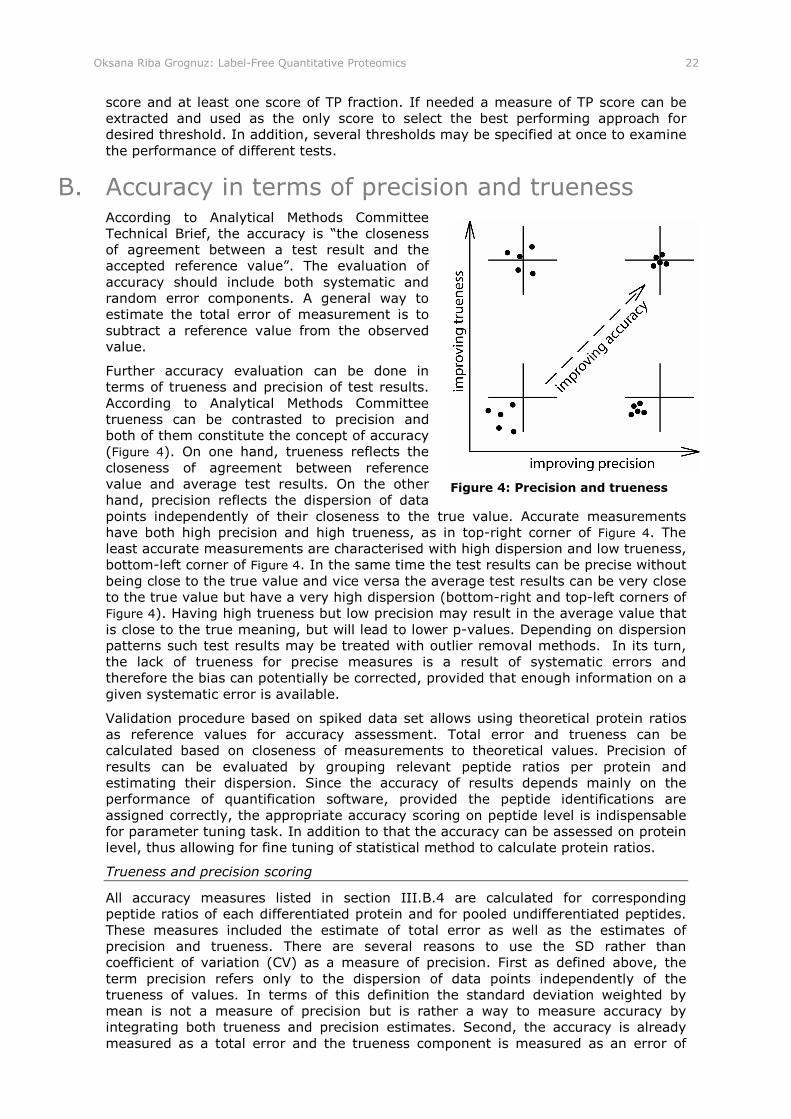
Oksana Riba Grognuz: Label-Free Quantitative Proteomics 22
score and at least one score of TP fraction. If needed a measure of TP score can be extracted and used as the only score to select the best performing approach for desired threshold. In addition, several thresholds may be specified at once to examine the performance of different tests.
B. Accuracy in terms of precision and trueness According to Analytical Methods Committee Technical Brief, the accuracy is “the closeness of agreement between a test result and the accepted reference value”. The evaluation of accuracy should include both systematic and random error components. A general way to estimate the total error of measurement is to subtract a reference value from the observed value.
Further accuracy evaluation can be done in terms of trueness and precision of test results. According to Analytical Methods Committee trueness can be contrasted to precision and both of them constitute the concept of accuracy (Figure 4). On one hand, trueness reflects the closeness of agreement between reference value and average test results. On the other hand, precision reflects the dispersion of data points independently of their closeness to the true value. Accurate measurements have both high precision and high trueness, as in top-right corner of Figure 4. The least accurate measurements are characterised with high dispersion and low trueness, bottom-left corner of Figure 4. In the same time the test results can be precise without being close to the true value and vice versa the average test results can be very close to the true value but have a very high dispersion (bottom-right and top-left corners of Figure 4). Having high trueness but low precision may result in the average value that is close to the true meaning, but will lead to lower p-values. Depending on dispersion patterns such test results may be treated with outlier removal methods. In its turn, the lack of trueness for precise measures is a result of systematic errors and therefore the bias can potentially be corrected, provided that enough information on a given systematic error is available.
Validation procedure based on spiked data set allows using theoretical protein ratios as reference values for accuracy assessment. Total error and trueness can be calculated based on closeness of measurements to theoretical values. Precision of results can be evaluated by grouping relevant peptide ratios per protein and estimating their dispersion. Since the accuracy of results depends mainly on the performance of quantification software, provided the peptide identifications are assigned correctly, the appropriate accuracy scoring on peptide level is indispensable for parameter tuning task. In addition to that the accuracy can be assessed on protein level, thus allowing for fine tuning of statistical method to calculate protein ratios.
Trueness and precision scoring
All accuracy measures listed in section III.B.4 are calculated for corresponding peptide ratios of each differentiated protein and for pooled undifferentiated peptides. These measures included the estimate of total error as well as the estimates of precision and trueness. There are several reasons to use the SD rather than coefficient of variation (CV) as a measure of precision. First as defined above, the term precision refers only to the dispersion of data points independently of the trueness of values. In terms of this definition the standard deviation weighted by mean is not a measure of precision but is rather a way to measure accuracy by integrating both trueness and precision estimates. Second, the accuracy is already measured as a total error and the trueness component is measured as an error of
Figure 4: Precision and trueness

Oksana Riba Grognuz: Label-Free Quantitative Proteomics 23
nT.P CV score �
Score absolute mean median SD mean dev. trueness trueness
The validation data set mimics four accuracy cases displayed in Figure 4: T.P, TnP, nT.nP, nTnP
T=true, P=precise, nT=not true, nP=not precise
Figure 6: Validation of accuracy scoring: sub-scores for trueness and precision measures of validation data set
Total T.P TnP nT.P nTnP Score test test test test
T=true, P=precise, nT=not true, nP=not precise
Figure 5: Effect of SD sub-score weight on scoring performance
mean and median results. Finally, the use of CV will penalize the cases when the theoretical ratio is detected with better trueness in favour of the cases with equivalent standard deviation, but bigger observed mean ratio. Therefore the SD is used as a measure of precision to complement the measures of trueness and total error included in the scoring function.
To validate the performance of suggested scoring function, the validation data set included four cases displayed in Figure 4 (Appendix, Table 13):
1. Results with high trueness and precision (test T.P)
2. Results with high trueness, but low precision (test TnP)
3. Results with low trueness and high precision (test nT.P)
4. Results with low trueness and low precision (test nTnP)
Final accuracy sub-scores calculated for each accuracy measure as defined in section III.B.4 and total scores are provided in Appendix Table 14. Figure
6 shows that the test with high trueness and precision yields the best absolute mean deviation score. Trueness of geometric mean and median scores are equivalent for both tests with high trueness. SD score is the same for both tests that have high precision. Thus the most accurate test (T.P) has the highest sub-score only for the measure of total error that reflects both accuracy sides: precision and trueness.
As expected, the true and precise test yields the best total score (Figure 5, weight 1). However the middle cases when either trueness or precision is lacking do not yield equivalent scores. The test that is precise but lacks trueness has three times lower score than the test with high trueness but low precision. Accuracy scoring includes two trueness measures against one precision measure. Measuring the accuracy of mean and median is advantageous as depending on the data the accuracy may be high only for one of these measures. Therefore if one needs to promote the scoring of precise tests, then the weight coefficients can be assigned to sub-scores. Thus assigning a weight
of 2 to SD score and 1 to all remaining sub scores to compensate the presence of two measures of trueness will favour the precise test nT.P lacking trueness (Figure 5, weight 2).
The spiked data set analysed with different parameters will yield the results having varying precision and trueness, and it is unlikely that there will be one result having both high precision and high trueness in comparison to all others. Thus depending on the particular goals precise tests may be important to favour. A way to assign a weight coefficient is thus provided to allow for better flexibility of scoring function.

Oksana Riba Grognuz: Label-Free Quantitative Proteomics 24
V. Results The developed pipeline provides for a common statistical and processing framework for different label-free proteomics software. The pipeline consists of the three building blocks: quantification, statistical analysis and accuracy analysis (Figure 7).
The quantification block contains the integrated quantitative software packages. The target software should be incorporated in the automated processing flow and supplemented with an appropriate converter for generated list of features. The initial design of the pipeline included two software packages: SpecArray and SuperHirn (section II.C.2). As for most open source programs, the input files to quantitative block are the spectra data converted to mzXML format and MS/MS identification information converted into pep.xml format (Figure 7). In addition an input file with relevant parameter settings is required for parameter tuning based on spiked data set.
Quantification software is used to produce feature lists, which are then converted to a common format and submitted for further analysis in statistical analysis block (Figure
7). An additional user input is required to describe samples by providing the sample names and the list of file names without extensions for each relevant replicate MS run. This part performs a series of statistical tests to characterise data and estimate the evidence for differential expression. The output of statistical analysis includes result tables for peptides and proteins with their respective ratios, p-values and other measures, such as coefficient of variation. All calculated data is also exported into an R data object, containing all measures and indexes for different thresholds and characteristics. Thus any of the measures can be explored further in R environment. In addition a plotting module was developed with a set of plotting functions to explore data quality and patterns.
R object generated in statistical analysis can be submitted for accuracy analysis (Figure 7). All functions included in accuracy analysis are applicable for spiked experiments, if spiked protein concentrations are provided as input. A part of available analytical tools can be used for all experiments, such as ROC analysis and overall comparison of experiments (e.g. total number of extracted features, complete features etc.). The accuracy analysis generates type I and II error plots, score plots and ROC plots in both ROC and density space. The scores and ROC data are also exported as R objects. In addition a table combining the indicators of performance for different experiments is created.
The pipeline was first validated with test data set containing four spiked proteins at known ratios. The optimal parameter settings for LTQ-Orbitrap platform were determined in parameterisation analysis. The validated pipeline was then applied to biological samples using the selected optimal parameters.
A. Software Parameterisation The parameterisation analysis allowed tuning software parameter settings to achieve the improved performance on LTQ-Orbitrap platform. In addition it revealed the
Figure 7: Framework overview

Oksana Riba Grognuz: Label-Free Quantitative Proteomics 25
parameters that are critical for feature extraction and has given an insight on their influence. The main goal of SpecArray parameter tuning is to adapt the package developed for Q-TOF mass analyzer for the analysis of high resolution data. In case of SuperHirn, the main goal is to reduce the redundancy of extracted features. SuperHirn algorithm has a tendency of detecting the same feature for several times within a very narrow time (starting from 0.05 minutes) and mass-to-charge ratio (less than 1 ppm) interval.
A number of different parameter settings were tested for each program. The selected parameters included mass-to-charge ratio peak width, mass-to-charge ratio differences between scans and between runs, retention time window, retention time differences between runs (illustrated in Figure 8) and the maximum number of scans that can be between members of an LC elution peak. The tested approaches were assessed for results precision and trueness (accuracy scoring) as well as for their capacity to distinguish correctly differentially expressed features (ROC-based scoring), see section IV. As ROC-based scoring implements the widely accepted approach for test performance assessment the best scoring tests were first selected by their ROC-based scores for t-test p-value and fold-change classifiers and then these tests were compared by their accuracy score values. Both performance evaluations were based on known identities and concentrations of spiked peptides and on Mascot identifications assignments to the extracted features. Thus a given feature is considered as differentially expressed, if it is identified as a peptide of one of the spiked proteins. Therefore the measures of performance depend on the quality of the identification assignment.
1. SpecArray
Individual and combinatory effects of six parameters listed in section III.C were assessed with twenty-nine parameter settings that included the default parameters (Appendix, Table 15). The score values for four best tests determined with this approach and for the test with default values (test 1) are shown in Figure 9 displaying the accuracy sub-scores and Figure 10 displaying the ROC sub-scores for the performance of two classifiers: t-test p-values (Figure 10A) and fold-change (Figure 10B). In terms of accuracy scores, tests 13 and 19 lead in all cases. Although for mean accuracy all four selected tests have the equivalent performance. For all accuracy measures the selected best scores have much better performance than the default test 1. In terms of ROC-based scores, the improvement in AUC for the selected tests is not
200 -
150 -
100 -
50 –
0 - Score abs. mean median SD mean true- true- dev. ness ness
Default parameters = test 1
Figure 9: SpecArray accuracy sub-scores for different parameter settings (Table 15)
Test 1 Test 13 Test 19 Test 22 Test 27
Figure 8: Types of tested parameters based on intensity, mass-to-charge ratio and retention time
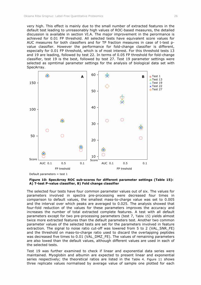
Oksana Riba Grognuz: Label-Free Quantitative Proteomics 26
very high. This effect is mainly due to the small number of extracted features in the default test leading to unreasonably high values of ROC-based measures, the detailed discussion is available in section VI.A. The major improvement in the perormance is achieved for 0.01 FP threshold. All selected tests have equivalent score values for AUC measures for both classifiers and for TP fraction measures in case of t-test p-value classifier. However the performance for fold-change classifier is different, especially for 0.01 FP threshold, which is of most interest. For this threshold tests 13 and 19 are leading, followed by test 22. In terms of 0.05 FP threshold for fold-change classifier, test 19 is the best, followed by test 27. Test 19 parameter settings were selected as opmtimal parameter settings for the analysis of biological data set with SpecArray.
The selected four tests have four common parameter values out of six. The values for parameters involved in spectra pre-processing were decreased four times in comparison to default values, the smallest mass-to-charge value was set to 0.005 and the interval over which peaks are averaged to 0.025. The analysis showed that four-fold reduction of the values for these parameters improves the accuracy and increases the number of total extracted complete features. A test with all default parameters except for two pre-processing parameters (test 7, Table 15) yields almost twice more extracted features than the default parameters test. Another two common parameter values of the selected tests are set for the parameters involved in feature extraction. The signal to noise ratio cut-off was lowered from 5 to 2 (VAL_SNR_FE) and the threshold on mass-to-charge ratio used to discard the overlapping peptides was decreased five times to 0.01 (VAL_DMZ_FE). The values of remaining parameters are also lowed than the default values, although different values are used in each of the selected tests.
Test 19 was further examined to check if linear and exponential data series were maintained. Myoglobin and albumin are expected to present linear and exponential series respectively; the theoretical ratios are listed in the Table 4. Figure 11 shows three replicate values normalised by average value of sample one plotted for each
150 -
100 -
50 –
Score
AUC 0.1 0.5 0.1 AUC 0.1 0.5 0.1
FP treshold FP treshold
Default parameters = test 1
Figure 10: SpecArray ROC sub-scores for different parameter settings (Table 15): A) T-test P-value classifier, B) Fold change classifier
A
B 60 -
50 -
40 -
30 –
20 –
10 - Score
Test 1 Test 13 Test 19 Test 22 Test 27

Oksana Riba Grognuz: Label-Free Quantitative Proteomics 27
sample. Mean and median values are indicated with plus and cross signs. The replicate points are rather dispersed, although the respective mean and median values approximate the expected linear and exponential patterns. Similar patterns are observed for most of the peptides assigned with albumin or myoglobin identification.
Figure 12 shows the scatter plot of features quantified with default parameter settings (test 1) and using the parameter settings of test 19, selected as optimal. Under the default parameters only 1096 features are extracted. Albumin is the only differentially expressed protein that has measured relative abundance for sample 2 over 1 with three peptide ratios. The results of test 19 contain 2265 extracted complete features, more than twice as much as default test. Test 19 measures the relative abundance of features that were assigned to three out of four differentially expressed proteins in sample 2 over 1. The measured ratios are clustered around the expected theoretical values. The smallest ratio of 0.7 for casein is not detected with any of the tested approaches. The smallest detected ratio is 0.66 (not on the plot).
A B
Figure 12: Sample 2 versus sample 1 feature fold change using different parameter settings of SpecArray: A) default parameters (test 1, Table 15), B) optimal parameters (test 19, Table 15)
log2(ratio) feature# log2(ratio) feature# (increasing m/z order) (increasing m/z order)
Theoretical ratios for differentiated proteins are indicated on the left of the plot in respective colour
ECOLI ECOLI
Figure 11: Feature ratio measurement in linear and exponential series by SpecArray with optimal parameter settings (test 19, Table 15)
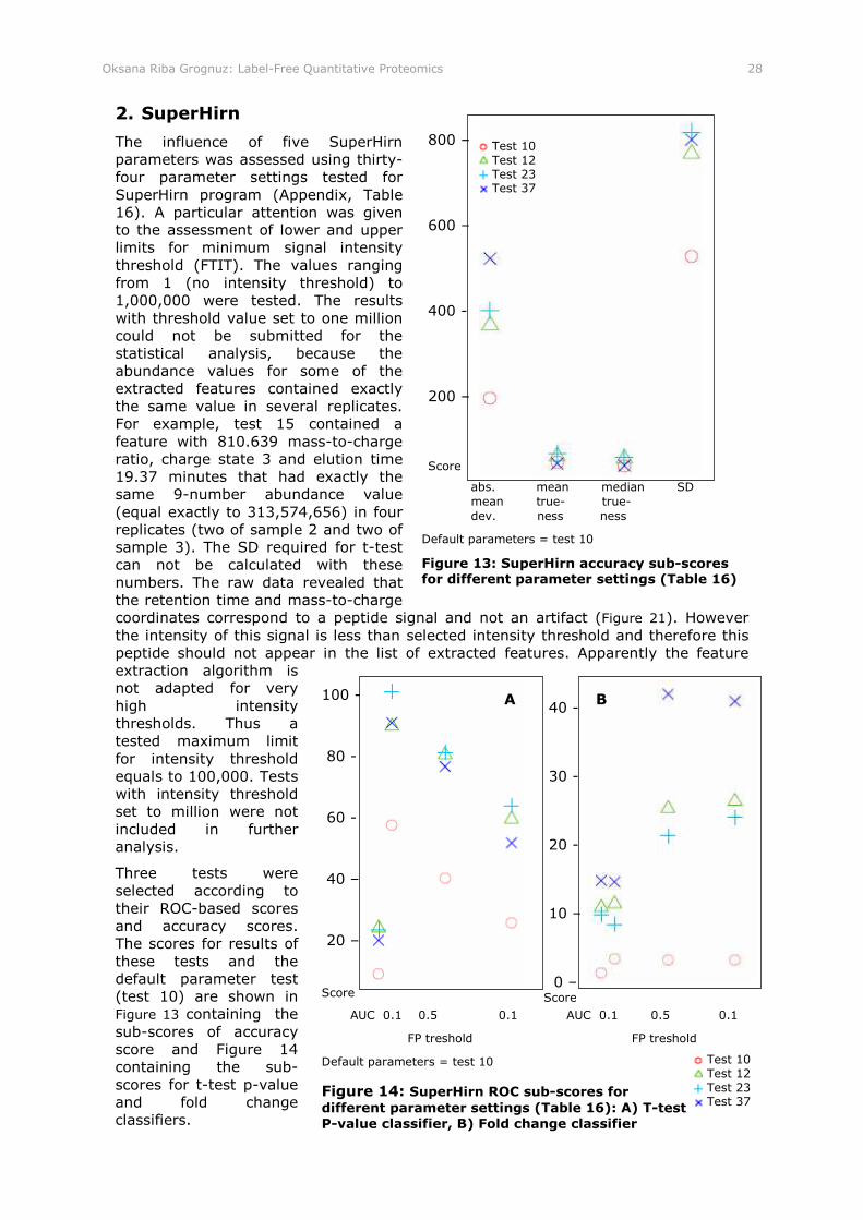
Oksana Riba Grognuz: Label-Free Quantitative Proteomics 28
Test 10 Test 12 Test 23 Test 37
100 -
80 -
60 -
40 –
20 –
Score
AUC 0.1 0.5 0.1 AUC 0.1 0.5 0.1
FP treshold FP treshold
Default parameters = test 10
A 40 -
30 -
20 -
10 –
0 – Score
Figure 14: SuperHirn ROC sub-scores for different parameter settings (Table 16): A) T-test P-value classifier, B) Fold change classifier
B
800 –
600 –
400 -
200 –
Score
abs. mean median SD mean true- true- dev. ness ness
Default parameters = test 10
Figure 13: SuperHirn accuracy sub-scores for different parameter settings (Table 16)
Test 10 Test 12 Test 23 Test 37
2. SuperHirn
The influence of five SuperHirn parameters was assessed using thirty-four parameter settings tested for SuperHirn program (Appendix, Table 16). A particular attention was given to the assessment of lower and upper limits for minimum signal intensity threshold (FTIT). The values ranging from 1 (no intensity threshold) to 1,000,000 were tested. The results with threshold value set to one million could not be submitted for the statistical analysis, because the abundance values for some of the extracted features contained exactly the same value in several replicates. For example, test 15 contained a feature with 810.639 mass-to-charge ratio, charge state 3 and elution time 19.37 minutes that had exactly the same 9-number abundance value (equal exactly to 313,574,656) in four replicates (two of sample 2 and two of sample 3). The SD required for t-test can not be calculated with these numbers. The raw data revealed that the retention time and mass-to-charge coordinates correspond to a peptide signal and not an artifact (Figure 21). However the intensity of this signal is less than selected intensity threshold and therefore this peptide should not appear in the list of extracted features. Apparently the feature extraction algorithm is not adapted for very high intensity thresholds. Thus a tested maximum limit for intensity threshold equals to 100,000. Tests with intensity threshold set to million were not included in further analysis.
Three tests were selected according to their ROC-based scores and accuracy scores. The scores for results of these tests and the default parameter test (test 10) are shown in Figure 13 containing the sub-scores of accuracy score and Figure 14 containing the sub-scores for t-test p-value and fold change classifiers.
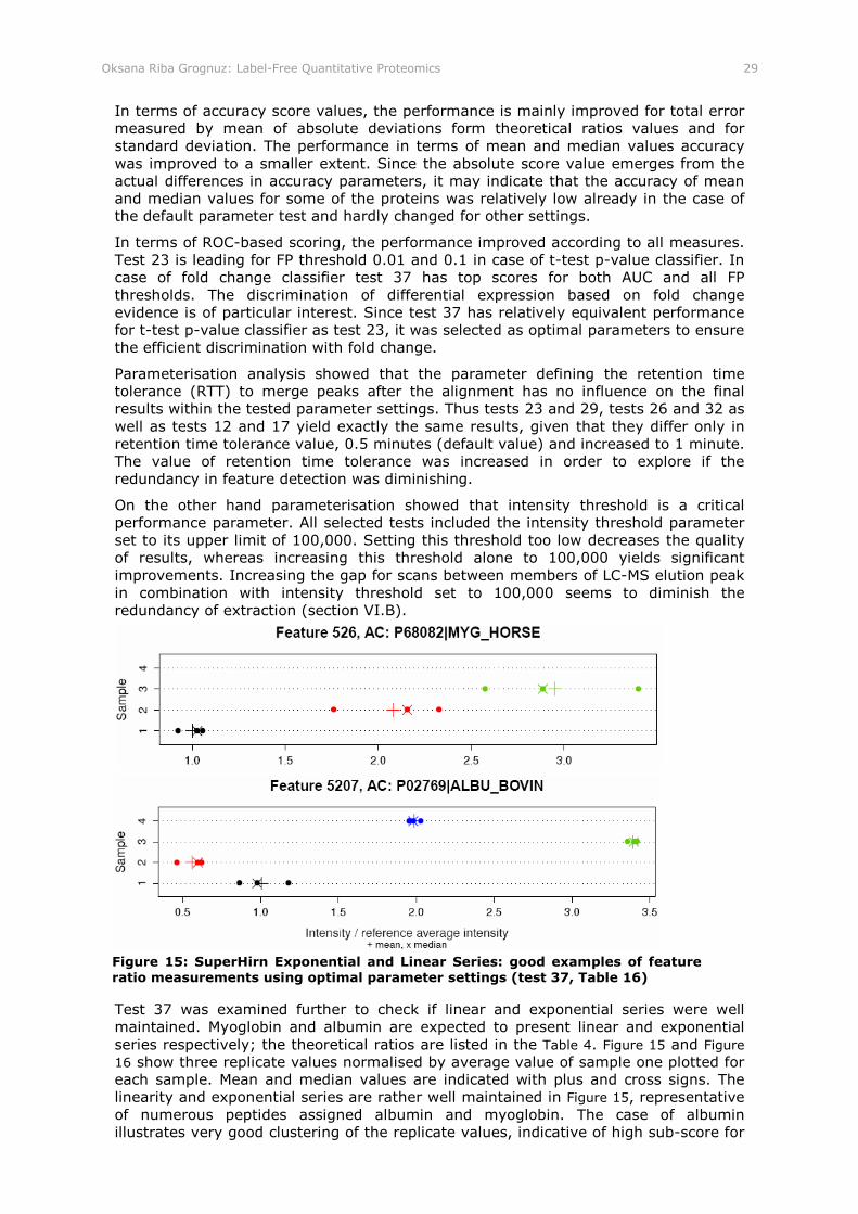
Oksana Riba Grognuz: Label-Free Quantitative Proteomics 29
In terms of accuracy score values, the performance is mainly improved for total error measured by mean of absolute deviations form theoretical ratios values and for standard deviation. The performance in terms of mean and median values accuracy was improved to a smaller extent. Since the absolute score value emerges from the actual differences in accuracy parameters, it may indicate that the accuracy of mean and median values for some of the proteins was relatively low already in the case of the default parameter test and hardly changed for other settings.
In terms of ROC-based scoring, the performance improved according to all measures. Test 23 is leading for FP threshold 0.01 and 0.1 in case of t-test p-value classifier. In case of fold change classifier test 37 has top scores for both AUC and all FP thresholds. The discrimination of differential expression based on fold change evidence is of particular interest. Since test 37 has relatively equivalent performance for t-test p-value classifier as test 23, it was selected as optimal parameters to ensure the efficient discrimination with fold change.
Parameterisation analysis showed that the parameter defining the retention time tolerance (RTT) to merge peaks after the alignment has no influence on the final results within the tested parameter settings. Thus tests 23 and 29, tests 26 and 32 as well as tests 12 and 17 yield exactly the same results, given that they differ only in retention time tolerance value, 0.5 minutes (default value) and increased to 1 minute. The value of retention time tolerance was increased in order to explore if the redundancy in feature detection was diminishing.
On the other hand parameterisation showed that intensity threshold is a critical performance parameter. All selected tests included the intensity threshold parameter set to its upper limit of 100,000. Setting this threshold too low decreases the quality of results, whereas increasing this threshold alone to 100,000 yields significant improvements. Increasing the gap for scans between members of LC-MS elution peak in combination with intensity threshold set to 100,000 seems to diminish the redundancy of extraction (section VI.B).
Test 37 was examined further to check if linear and exponential series were well maintained. Myoglobin and albumin are expected to present linear and exponential series respectively; the theoretical ratios are listed in the Table 4. Figure 15 and Figure
16 show three replicate values normalised by average value of sample one plotted for each sample. Mean and median values are indicated with plus and cross signs. The linearity and exponential series are rather well maintained in Figure 15, representative of numerous peptides assigned albumin and myoglobin. The case of albumin illustrates very good clustering of the replicate values, indicative of high sub-score for
Figure 15: SuperHirn Exponential and Linear Series: good examples of feature
ratio measurements using optimal parameter settings (test 37, Table 16)

Oksana Riba Grognuz: Label-Free Quantitative Proteomics 30
standard deviation. However there are also present the cases when the dispersion is very big as in Figure 16 illustrating the observed cases when linear and exponential
series of features assigned to myoglobin or albumin are not maintained. The possible reason for that is not necessarily the bad intensity integration or peak during feature extraction, but the erroneous identification of feature. The identifications originate from Mascot search done for MS/MS spectra. The error may occur not only in Mascot identification itself, but also be produced during SuperHirn processing of Mascot identifications. A detailed discussion is available in section VI.C.
Figure 17 shows the performance of SuperHirn with default parameters (test 10) and with optimal settings selected in parameterisation analysis. Test 37 differs from default parameters in three parameter values: ten times higher intensity threshold (100,000), two-times bigger inter-scan distance of members of an LC-MS elution peak and two times lower mass-to-charge threshold for peak clustering during detection. Default test extracts 56,613 features out of which some 25% are present in all replicates of at least one sample. Test 37 extracts 34,286 features out of which 28% are present in all replicates of at least one sample. The coverage of differentiated proteins is maintained despite the reduction in the number of extracted features,
Figure 16: SuperHirn Exponential and Linear Series: bad examples of feature
ratio measurements using optimal parameter settings (test 37, Table 16)
test 10
test 37
log2(ratio) log2(ratio)
Figure 17: Sample 2 versus sample 1 feature fold change using different parameter settings of SuperHirn: A) default parameters (test 10, Table 16), B) optimal parameters (test 37, Table 16)
Theoretical ratios for differentiated proteins are indicated on the left of the plot in respective colour
feature# (increasing m/z order)
feature# (increasing m/z order)
A B
ECOLI ECOLI
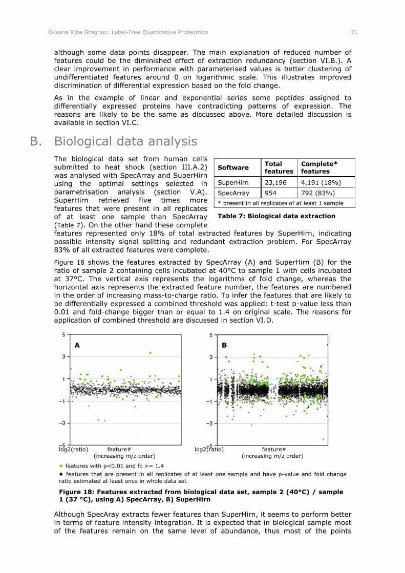
Oksana Riba Grognuz: Label-Free Quantitative Proteomics 31
although some data points disappear. The main explanation of reduced number of features could be the diminished effect of extraction redundancy (section VI.B.). A clear improvement in performance with parameterised values is better clustering of undifferentiated features around 0 on logarithmic scale. This illustrates improved discrimination of differential expression based on the fold change.
As in the example of linear and exponential series some peptides assigned to differentially expressed proteins have contradicting patterns of expression. The reasons are likely to be the same as discussed above. More detailed discussion is available in section VI.C.
B. Biological data analysis
The biological data set from human cells submitted to heat shock (section III.A.2) was analysed with SpecArray and SuperHirn using the optimal settings selected in parametrisation analysis (section V.A). SuperHirn retrieved five times more features that were present in all replicates of at least one sample than SpecArray (Table 7). On the other hand these complete features represented only 18% of total extracted features by SuperHirn, indicating possible intensity signal splitting and redundant extraction problem. For SpecArray 83% of all extracted features were complete.
Figure 18 shows the features extracted by SpecArray (A) and SuperHirn (B) for the ratio of sample 2 containing cells incubated at 40°C to sample 1 with cells incubated at 37°C. The vertical axis represents the logarithms of fold change, whereas the horizontal axis represents the extracted feature number, the features are numbered in the order of increasing mass-to-charge ratio. To infer the features that are likely to be differentially expressed a combined threshold was applied: t-test p-value less than 0.01 and fold-change bigger than or equal to 1.4 on original scale. The reasons for application of combined threshold are discussed in section VI.D.
Although SpecAray extracts fewer features than SuperHirn, it seems to perform better in terms of feature intensity integration. It is expected that in biological sample most of the features remain on the same level of abundance, thus most of the points
Software Total features
Complete* features
SuperHirn 23,196 4,191 (18%)
SpecArray 954 792 (83%)
* present in all replicates of at least 1 sample
Table 7: Biological data extraction
log2(ratio) feature# log2(ratio) feature# (increasing m/z order) (increasing m/z order)
● features with p<0.01 and fc >= 1.4
● features that are present in all replicates of at least one sample and have p-value and fold change ratio estimated at least once in whole data set
A B
Figure 18: Features extracted from biological data set, sample 2 (40°C) / sample 1 (37 °C), using A) SpecArray, B) SuperHirn

Oksana Riba Grognuz: Label-Free Quantitative Proteomics 32
Figure 19: Protein identification overlap between SpecArray and SuperHirn
should be clustered around zero on vertical axis. Most of the features extracted in SpecArray are rather well clustered around zero (Figure 18 A), whereas SuperHirn yields rather wide dispersion of measured fold change ratios (Figure 18 B). The reason for this could be related to the differences in the implemented approaches for intensity integration. SpecArray integrates the intensity of three isotopes and discards the overlapping peptides within a defined retention time and mass-to-charge interval (section II.C.2.a). SuperHirn derives the abundance information from the intensity of the monoisotopic peak and applies the algorithm to resolve the overlapping patterns.
The benefit of SuperHirn is the high number of extracted features including those of lower intensity. On the other side there is a risk of high number of redundant extractions and signal splitting. The gaps in the scatter plot in Figure 18 B, indicate the regions where the incomplete features (features that are not present in all replicates of at least one sample) were filtered out. The biggest amount of incomplete features seems to be located around middle mass-to-charge values. For example, features of mass-to-charge ratio close to 650 are subject to high number of missing abundance values. In addition smaller gaps are visible in the left part of the scatter plot, corresponding to small mass-to-charge measurements.
To further evaluate the performance of the two integrated software, the identified features were grouped to proteins. SuperHirn detects and quantifies more features and consequently more proteins than SpecArray. The numbers of proteins that have at least one peptide present in all replicates of one sample were compared (Figure 19). SuperHirn results contain 369 proteins, whereas SpecArray results contain 202 proteins, out of which 191 proteins are found by both programs.
In order to infer the proteins that are likely to be differentially expressed in given biological samples, a threshold of 1.4 was applied on fold change ratio and a threshold of 0.05 was applied on p-value calculated with one-sided t-test on protein
Protein AC SW N.pp FC CV P-value
SA 3 1.97 0.12 8.36*10-3 HS905_HUMAN*
SH 3 1.53 0.05 4.23*10-3
SA 10 1.82 0.23 6.83*10-5 HS90A_HUMAN*
SH 19 1.43 0.22 1.51*10-7
SA 4 7.90 NA NA HSP71_HUMAN**
SH 14 2.00 0.55 2.46*10-4
SA 1 2.32 NA NA HS105_HUMAN**
SH 12 1.55 0.23 2.48*10-6
SA 5 0.46 0.60 9.82*10-1 HS71L_HUMAN**
SH 7 4.84 0.70 2.35*10-3
SA 4 1.83 0.39 1.76*10-1 CHRD1_HUMAN**
SH 7 1.78 0.30 4.10*10-3
SA 1 1.46 NA NA XPP3_HUMAN**
SH 1 1.51 NA NA * p-value<0.05, FC>=1.4 ** FC>=1.4 SW=software, N.pp=number of peptides, FC=fold change, CV=coefficient of variation, SA=SpecArray, SH=SuperHirn.
Table 8: Protein differential expression assignment overlap in sample 2 (40°C) / sample 1 (37°C) between SpecArray and SuperHirn
Oksana Riba Grognuz: Label-Free Quantitative Proteomics 33
level, null hypothesis is that the mean ratio of relevant peptides is equal to 0. Based on these cut-offs SuperHirn yielded 7 and SpecArray 5 proteins that are likely to be differentially expressed (Figure 19). Two of these proteins were assigned significance by both SpecArray and SuperHirn.
By applying a threshold of fold change alone, 7 assignments of differential expression overlap between 43 total SuperHirn assignments and 18 total SpecArray assignments (Figure 19). Table 8 lists the overlapping proteins and their corresponding ratios, number of peptides per protein, p-values and coefficients of variation for fold-change threshold alone that includes the two overlapping proteins found with combined threshold.
As expected the list of proteins that are likely to be differentially expressed includes heat shock proteins. The two proteins found by application of both t-test p-value and fold change thresholds, HS905_HUMAN and HS90A_HUMAN belong to heat shock protein 90 family according to general annotation in relevant Swiss-Prot entries (Table
8). HSP71_HUMAN, HS105_HUMAN and HS71L_HUMAN belong to heat shock protein 70 family. CHRD1_HUMAN interacts with heat shock proteins HSP90AA1 and HSP90AB1 in an ATP-independent manner. The only protein that does not seem to play a clear role in heat shock is aminopeptidase XPP3_HUMAN. However there is only one unique peptide assigned to this protein in both SpecArray and SuperHirn results and no shared peptides are present. Therefore the level of uncertainty regarding the differential expression of XPP3 is rather high.
Two overlapping proteins in differential protein lists retrieved by SpecArray and SuperHirn using a combined threshold have shared peptides. The three peptides assigned to HS905 are also assigned to HS90A. In order to deal with cases of multiple peptide identification assignments, the peptide was attributed to the first identification in the list. Therefore the three peptides assigned to HS905 may actually belong to HS90A. High sequence similarity of heat shock proteins hinders the task of peptide grouping to proteins. From the list of peptides that may possibly belong to HS90A, there are some 10 peptides in SpecArray results and some 20 peptides in SuperHirn results assigned uniquely to HS90A. Other peptides are shared by up to five proteins in the same time.
Protein HSP71_HUMAN that is retrieved by double threshold from SuperHirn results has missing p-value and coefficient of variation in SpecArray results, although 4 peptides are assigned to this protein. The examination of relevant peptides showed that 3 out of 4 peptides are not detected in sample 1 at 37°C and therefore result in missing p-value for the ratio of sample at 40°C versus 37°C. Since SpecArray uses hard-coded threshold on signal intensity, it is possible that some low intensity peptide signals are simply filtered out and are detected only when their intensity level increases. Thus protein HSP71_HUMAN had only 1 peptide assigned to it in sample 1 at 37°C and 4 peptides in sample 2 at 40°C.
In addition, only 3 SpecArray features are identified as unique HSP71_HUMAN protein peptides. This matches the Mascot search that finds 3 peptides assigned only to HSP71_HUMAN in three replicates of sample 1 at 37°C. Other peptides assigned to HSP71 are also assigned to other proteins, for example to HSP7C, to which Mascot assigns more than twenty peptides. It is possible that more of the shared peptides belong to HSP71, but the inference of these peptides requires additional analysis.
The ratios retrieved for HSP71 by SpecArray and SuperHirn differ a lot. With the only 1 quantified peptide in both samples, SpecArray estimates the fold change of 7.9, whereas SuperHirn results yield a fold change of 2. On one side SuperHirn yields more peptides for the given protein and could potentially produce more reliable results, however the corresponding CV in Table 8 is more than 50% and therefore could indicate the problem of peptide grouping. Out of all peptides that are assigned to HSP71 in SuperHirn results, 12 are assigned only to the given protein, although 3 of these features seem to be the redundant extractions of the same peptide peak. The fold change ratio of peptides assigned exclusively to HSP71 range from 3.4 to 7.6, whereas the ratios of peptides with several identifications range from 1.3 to 13.2.

Oksana Riba Grognuz: Label-Free Quantitative Proteomics 34
Thus it is possible that the true ratio of HSP71 is bigger than 2, provided that some of the assigned peptides belong to another protein.
In addition, redundant feature extraction by SuperHirn in some cases leads to intensity signal splitting and thus may impede the calculation of some ratios. A four-time charged peptide assigned only to HSP71 protein seems to be extracted as three different features with maximum time difference of 0.12 minutes and maximum mass-to-charge difference of 1.5 ppm. As shown in Table 9, the feature present at 37°C is not detected at 40°C, whereas two features detected at 40°C are not present at 37°C. Moreover at 40°C the detected intensity level is similar for both features, although none of these features has observations in all replicates. It seems that intensity signal is split among the redundant extractions of the same peptide. If these three features would be combined to one feature, then the fold change of sample 2 (40°C) to 1 (37°C) could be calculated, provided that the abundance estimate is present in all replicates of sample 2 and in one replicate of sample 1.
m/z Rt z 37°C, log2(intensity) 40°C, log2(intensity)
666.316 45.3 4 - - - - - - 28.27 27.84
666.3164 45.31 4 25.15 - - - - - - -
666.317 45.42 4 - - - - 28.46 28.73 - 27.63
Table 9: SuperHirn redundant extraction of feature assigned to HSP71_HUMAN

Oksana Riba Grognuz: Label-Free Quantitative Proteomics 35
VI. Discussion The main goal of SpecArray parameterisation was to increase the number of extracted features while maintaining the sufficient quality of the results. Given the low number of extracted differentiated peptides, the use of both types of accuracy scoring implemented within a pipeline may lead to misleading results. To avoid high scoring of limited feature output, all SpecArray scores were adjusted by the coefficient based on the number of extracted features. The optimal settings determined during the parameterisation allowed increasing more than twice the number of extractions. However even the parameterised SpecArray quantification fails to achieve the equivalent level of extraction as SuperHirn. The latter one retrieves about five times more features present in all replicates of at leas one sample for the same data set. Though SuperHirn extraction is probably excessive as the same peptide peak can be extracted several features within a narrow mass and time interval. Such redundancy may be problematic for quantification if the intensity signal is split among the repeated extractions.
The parameterisation analysis relied on the assigned peptide identities to distinguish the differentiated peptides from undifferentiated ones. The results of performance assessment thus depend on the quality of identification. In case of SpecArray the identifications were parsed by using threshold on mass-to-charge ratio, retention time and Mascot ion score. SuperHirn processes the pep.xml files provided as input and assigns probabilities to peptide identifications. The final lists of extracted features were filtered by applying a threshold on probability to remove the low probability identifications. However, especially in the results of SuperHirn some peptides assigned to the same protein had conflicting ratios. One hand there could be a problem during intensity integration. On the other hand the peptides may actually belong to another protein.
The biological data set was quantified using the determined optimal settings for SpecArray and SuperHirn. In order to infer the biologically significant differences in expression a combined threshold was applied on both t-test p-value and fold change ratio. The use of each of these thresholds separately is related to a number of issues discussed in section VI.D. The results of biological data set analysis confirmed the limitations of each quantification program determined during the test data set analyses. In addition, the biological data results accentuated the problem of peptide grouping to proteins, especially significant for heat shock proteins that have a lot of sequence similarities.
A. Adjusting SpecArray scores SpecArray score values were adjusted by the coefficient based on the number of total extracted complete features. The reason for this is the need to integrate the measure of the number of extracted features in the scoring results in order to find the approach that extracts the maximum possible number of peptides, while keeping the accuracy at the optimal level. SpecArray signal pre-processing and feature extraction are not adapted for high-resolution Orbitrap data and filter out valuable feature information as discussed in the section II.C.2.a. Without score adjustment the tests extracting only few differentially expressed peptides with accurate and precise values may yield high AUC and true positive fractions at selected thresholds in ROC analysis. If few detected peptides have high fold-change and low p-values then they will be distinguished from
log2(ratio) feature# (increasing m/z order)
Figure 20: Few differentiated peptides in default SpecArray results can yield maximal ROC measures
Sample 3/1, test 1
ECOLI

Oksana Riba Grognuz: Label-Free Quantitative Proteomics 36
undifferentiated ones at very low false positive thresholds. In addition, the accuracy scoring can be affected as well. The tests that do not cover all of the proteins will not have high scoring; however a test extracting only two peptides for most of proteins with significant accuracy can yield good precision and trueness measures.
An example of case when ROC-based measures are misleading is given in Figure 20. The figure shows the logarithms of ratios for sample 3 versus 1 for test data set quantified with default parameters (Appendix, Table 15, test 1). Three differentiated peptides are assigned to one spiked protein: albumin. The absolute value of logarithms of ratios of differentiated peptides is high enough to yield 99.(9)% AUC value, and 100% true positive fraction at FP thresholds of 0.01, 0.05, and 0.1 for fold change classifier. In addition these peptides have low p-values and yield same “perfect result” for p-value classifier. However this case is far to be perfect, with low number of detected features and only 3 peptides assigned to a differentiated protein.
Adjusting scoring values by a coefficient based on the total number of extracted features present in all replicates of at least one sample remedies this problem. Thus if without adjustment the best scoring tests include the tests with very low number of features, then after adjustment the tests with low number of features are no longer in the top of the list (Table 10). In the case of SuperHirn the score adjustment is not required, because the problem is presented by feature redundancy. Therefore approaches yielding the maximum number of extracted features are not necessarily the most efficient ones.
B. SuperHirn redundant extraction The redundancy of detection of the peptide, which induced feature extraction problems at one million intensity threshold, was assessed for two tests at no intensity threshold, for default parameter test (test 10) and three tests with 100,000 intensity threshold, including the selected optimal settings (Table 11). The tests were selected on order to assess the effect of the inter scan distance parameter (MISD) on the redundancy of the extraction at different intensity levels. Thus test 1 included in the Table 11 has all default parameters and no intensity threshold. Test 2 differs from test 1 in the value of MISD that was raised to 10. Default parameters (test 10) have intensity threshold equal to 10,000 and MISD equal to 5. The test 12 has all default parameters except for intensity level raised to 100,000. Test 26 differs from test 12 in the value of MISD raised to 10,
Posi-tion
No adjustment
With adjustment
1 Test 8 Test 13 2 Test 21 Test 19 3 Test 1 Test 22 4 Test 13 Test 27
5 Test 19 Test 29 6 Test 22 Test 24 7 Test 27 Test 21
Test 1 = default parameters Tests yielding low number of features
Table 10: Effect of SpecArray score adjustment based on the number of extracted features
Intensity = 4.65E5 Redundant extractions with default SuperHirn parameters
Figure 21: Example of redundantly extracted peptide
22.7 17.97
18.93
19.11 19.13
19.19 19.56
20.84
23.4
min

Oksana Riba Grognuz: Label-Free Quantitative Proteomics 37
Finally, the optimal settings (test 37) include 100,000 intensity threshold and MISD equal to 10.
Table 11 shows the extraction details for peptide with monoisotopic mass-to-charge ratio equal to 810.639, charge 3 and retention time equal to approximately 19 minutes. Figure 21 shows that the peak in raw data corresponding to these coordinates is likely to be a peptide, according to its isotopic distribution. The chromatographic elution profile seems to be of sufficient quality. The nine redundant extractions of the given peptide under default parameters are shown in Figure 21.
All tests have mass-to-charge ratio tolerance for peak clustering during extraction set to 0.01 m/z (default value) or lower (0.005 in optimal settings, test 37). The maximum difference in mass-to-charge values of redundantly extracted peptide is smaller than 1 ppm (about 0.007 m/z). Thus according to this threshold the redundant peptides should have been grouped together. On the other hand a retention time threshold for feature merge after the alignment is set to 0.5 minutes and the minimum difference in retention time for these features is small enough to group at least some of them together. The values for two aforementioned parameters do not seem to influence the redundancy in a significant way. Moreover retention time threshold did not yield any changes in results of the tested settings.
According to Table 11 setting an inter-scan distance to 10 seems to diminish the redundancy of extraction for given peptide. Simple reduction of intensity threshold to 1 (test 1) maintains the same number of repetitive extractions as in default test. However setting MISD to 10 even at no intensity threshold diminishes the number of repetitions to 5 (test 2). If the intensity threshold is set to 100,000 (test 12), the redundancy of a given feature increases. However if intensity threshold raise is supplemented with MISD raise to 10, the given peptide is extracted only once (optimal settings and test 26). Raising intensity and MISD values seems to reduce the number of extractions for some peptides.
One of the biggest problems induced by redundancy is splitting of abundance values. Thus minimum and maximum count columns in Table 11 show in how many replicates of all samples together (triplicates of 4 samples give 12 total cases possible) the abundance measure is extracted. In most of the cases the feature is extracted at least once in all 12 replicates; however the redundant extractions cover only some of the replicates. The abundance values for redundant peptides may be very intense at low count, while at lower intensity at maximum count. In addition the variability in replicate values seems to be rather important. The biological data set includes similar cases as test data set as discussed in section V.B.
C. Conflicting peptide ratios Figure 22 illustrates an example of conflicting albumin peptide ratios that are pointed with arrows. There are two main possible reasons behind this. On one hand the conflicting ratios may be due to the erroneous peptide intensity integration or peak picking. In case of SuperHirn the errors during feature extraction could be related to redundancy of extraction, especially if intensity signal is split. On the other hand the features may have a wrong assignment of identification. This may originate from
Test #
(Table
16)
times
extracted
max difference
in m/z (ppm)
min difference
in time (min)
min count
max count
MISD
1 9 0.97 0.05 2 12 5
2 5 0.37 0.31 1 12 10
10 9 0.97 0.08 2 12 5
12 11 0.86 0.15 1 12 5
26 1 - - 12 12 10
37 1 - - 12 12 10
Test 1: no intensity threshold Test 2: no intensity threshold Test 10: default parameters (intensity 10,000) Test 12: default + intensity threshold of 100,000 Test 26: intensity threshold of 100,000 Test 37: optimal parameters (intensity 100,000) MISD = # of scans between members of LC-peak
Table 11: The effect of MISD and intensity threshold on redundant feature extraction

Oksana Riba Grognuz: Label-Free Quantitative Proteomics 38
incorrect Mascot assignment or be attributable to SuperHirn processing of identifications submitted in pep.xml format.
Table 12 lists features in the same order (increasing mass-to-charge) as in Figure 22 A. There is a double extraction for 2nd and 3rd features. None of the extracted features is present in all twelve replicates of all samples pooled together (Table 12, column count). All peptide identifications are assigned a 100% probability by SuperHirn.
The best of the matched MS/MS spectra for peptide 1 is shown in Figure 22 B. Several peaks of high intensity are not assigned to peptide y or b fragment. The best matching spectra yields 18.4 Mascot ion score, whereas other MS/MS spectra for same feature yield lower Mascot score and also match some of the E.coli proteins. The Mascot assignments for this peptide may be erroneous because of the presence of unspecified modifications or absence of the given sequence in searched data base.
In its turn, SuperHirn processes all possible Mascot identifications to select the best available and estimates the probability of this identification. The case of peptide 1 illustrates that the 100% probability of identification can be assigned despite the fact that the best available Mascot ion score is relatively low.
One of the available MS/MS spectra for peptide 2 is shown in figure Figure 23 A. This spectrum yields rather
Figure 23: MS/MS spectrum of A) feature 2 B) feature 3 (Figure 22 A)
Mascot ion score: 45.6 for albumin
Mascot ion score: 42.3 for albumin
m/z
m/z
A
B
Figure 22: A) Conflicting albumin ratios in SuperHirn results for the test data
1 2
sample 2 / sample 1
B) MS/MS spectrum of feature 1
log2(ratio) feature# (increasing m/z order)
ECOLI
3
Mascot ion score: 18.4 for albumin
m/z
A B

Oksana Riba Grognuz: Label-Free Quantitative Proteomics 39
high Mascot ion score of 42.3, however few intense peaks are not assigned to peptide fragments. Other available spectra are of the similar quality. In this case again, the peptide may be wrongly identified by Mascot. However if the identification is correct, then the conflicting ratio may be the results of signal splitting during feature extraction. The feature 2 was detected twice within a narrow mass and time interval (Table 12).
The third peptide pointed in Figure 22 A has an ion score of 45.6 and a good quality matching for spectrum shown in Figure 23 B. All most intense ions are assigned to the respective peptide fragments. However,
despite the good quality of MS/MS spectra this peptide has the most conflicting ratio (Figure 22 A). The reason is probably related to SuperHirn feature extraction. On one hand the feature is extracted twice at relatively large mass-to-charge interval (5.6 ppm) and therefore could be due to low threshold on peak clustering during extraction (FTMZT, Test 37, Table 16). On the other hand the examination of raw data showed that the chromatographic elution profile is not of good quality. Thus it is possible that the extraction was hindered by poor quality of chromatogram.
D. Thresholds to infer differential expression As discussed in section II.D.2, in context of blind experiment the differential expression is inferred from the available evidence. First, the magnitude of fold change can be used to distinguish the features that are likely to be differentially expressed, the higher the magnitude, the higher the likelihood of differential expression. As illustrated in Figure 24 (figures C and D), applying fold change cut-off bigger or equal to 1.5 to ratios between samples 2 and 1 of test data set allows distinguishing almost all of the truly differentially expressed features quantified by either SpecArray or SuperHirn. However using only fold change cut-off results in high number of false positive results, which could possibly be due to other sources of variation, provided that the identifications were assigned correctly. Since only the identified features were included in Figure 24, the false positive results may belong to a spiked peptide only in the case of wrong assignment of MS/MS identification.
Another possibility to infer differential expression is through statistical analysis that supplements the fold change with the measure of data dispersion. Due to the reasons discussed in section II.D, a standard two-sided t-test was used to determine p-values. Setting a 0.01 p-value threshold allows detecting sufficient amount of truly differentiated features with lower number of false positive detections (Figure 24, A and B). The number of true positives is relatively equivalent in case of both types of thresholds, whereas the number of false positives is reduced significantly if p-value cut-off is applied.
Standard t-test does not take into account the magnitude of the fold-change. Thus, as illustrated in Figure 24 A and B, Ecoli peptides that have relatively small change in expression level are assigned low p-values. Any feature that has low dispersion within each of the samples will be assigned low p-value regardless of the magnitude of its fold change (Figure 25, A). Conversely, a feature with high dispersion in intensity values within each of the samples may be assigned a high p-value even if the fold change ratio is high (Figure 25, B).
m/z Rt z Sequence Probabilty count
501.7963 33.06 2 K.LVVSTQTALA 100% 11
740.4019 44.5 2 K.LGEYGFQNALIVR 100% 3
740.4042 44.97 2 K.LGEYGFQNALIVR 100% 10
978.4854 46.61 2 K.DAIPENLPPLTADFAEDK 100% 6
978.4909 45.22 2 K.DAIPENLPPLTADFAEDK 100% 3
Table 12: Three peptides assigned to albumin with comflicting ratios (Figure 22 A)

Oksana Riba Grognuz: Label-Free Quantitative Proteomics 40
A small scale fluctuation is in general more characteristic to biologically insignificant variation. A possible way to exclude the features with high p-values, but small fold-change is to apply a combined threshold. Thus only features with both low enough p-values and high enough fold-change ratio will be assigned significance in terms of differential expression. The problem of using the combined threshold is related to the determination of the fold-change threshold value. Depending on the sample the changes in expression level may be indeed of rather small scale. Thus failing to set a fold change threshold on low enough level may exclude truly differentially expressed features.
Another way to exclude the features with small fold-change is through the use of modified t-test. Limma t-statistics developed for microarray data considers the whole set of available fold change ratios to determine the lowest possible fold-change limit (section II.D.2.b). The features that have low dispersion but do not yield a high enough fold change ratio will be assigned higher p-values.
log2(ratio) log2(ratio)
log2(ratio) log2(ratio)
A B
C D
Figure 24: Ratios of peptides between two test samples assigned differential expression by applying a threshold on t-test p-value of SpecArray (A) and SuperHirn (B) results and by applying a fold change cutoff on SpecArray (C) and Superhirn (D)
Test data sample 2/1 Truly differentiated peptides are distinguished according to their identification as spiked protein peptides Truly undifferentiated peptides distinguished according to their identification as E.coli peptides
p-value<0.01 p-value<0.01
fc>=1.5
fc>=1.5
Figure 25: Problem using t-test: low p-values for small fold change (A) and high
p-values for big fold change (B)
mean 1mean 2
mean 1
mean 2
A
B

Oksana Riba Grognuz: Label-Free Quantitative Proteomics 41
E. Grouping peptides to proteins In order to deal with the cases of multiple peptide identification assignments, the peptide was attributed to the first identification in the list. Unfortunately, such simplistic approach cannot solve the problem of peptide grouping to proteins. On one side the order of multiple identifications listed in Mascot dat files reflects the likelihood of occurrence. Thus if peptide is shared between two proteins out of which one has a number of unique peptides and the other one has only shared peptides, the peptides will be assigned to the first protein. In this case indeed it is more likely that the first protein is present, although this does not mean that the second protein is absent. Bigger problem arises when two or more proteins have all shared peptides and represent thus equivalent identification possibilities. In this case the order in which possible identifications are listed does not represent any likelihood.
To provide for more elaborate procedure to deal with grouping issue, a mechanism of pattern examination could be developed to deduce the peptides that are likely to belong to other proteins than the ones they have been assigned to. Thus for example in cases when protein has some unique peptides and is assigned some of the shared peptides the patterns of fold change could be examined and strongly conflicting patterns could be excluded. In addition the examination of expression patterns for peptides shared among numerous proteins could in some cases provide an insight on the most probable number of proteins that could be present, by clustering the available patterns.

Oksana Riba Grognuz: Label-Free Quantitative Proteomics 42
VII. Conclusions The developed pipeline includes two quantification programs: SpecArray and SuperHirn and is readily extensible to include more programs. The pipeline provides means to evaluate the performance of the integrated software based on the data set with proteins at known concentrations. The software performance can be assessed in terms of capacity to distinguish the truly differentiated and undifferentiated peptides as well as in terms of trueness and precision of results. Critical performance parameters can be mapped and their influence can be investigated. In addition to software evaluation, the pipeline can be used to compare and combine the features extracted by different programs. The pipeline includes a number of statistical tools to analyse differential expression. All the aforementioned analyses do not require extensive informatics skills from a user, although provide for extended analysis options for experienced users.
Pipeline validation included the parameterisation analysis that allowed discerning the optimal parameter settings for both integrated software packages on LTQ-Orbitrap platform. The selected settings yield a better performance in terms of both ROC-based as well as trueness and precision measures. As expected the most critical SpecArray parameters are those that are involved in spectra pre-processing. The default thresholds, optimised for lower resolution data, induce a loss of feature signals when applied to higher resolution data. Thus a four-fold reduction of these parameters alone increases the number of extracted features. An additional increase seems to be attributable to a reduction of mass-to-charge threshold that is used to discard the overlapping features during the extraction. Other parameters are related to probability based retention time alignment and their influence is less clear. The most influential tested SuperHirn parameter is the threshold on intensity of the signal. Raising this threshold to 100,000 improves the analysis of data generated with Orbitrap.
The major benefit of the developed pipeline is the possibility to assess the limits and the benefits of different quantification software packages. Thus parameterised SpecArray quantifies features with rather small dispersion; most of resulting features remain on the same level of expression. However this advantage of SpecArray is associated with the limited number of quantified features in comparison to SuperHirn. A possible reason behind this could be related to hard-coded signal intensity cut-offs applied by SpecArray in spectra pre-processing. SuperHirn retrieves about five times more features present in all replicates of at least one sample than SpecArray, including low abundance features. However most of resulting abundance measures seem to be rather dispersed. In addition, the quality of final results is decreased by redundancy of feature extraction and intensity signal splitting. Although even with optimal SuperHirn settings the redundancy of extraction remains a problem, it seems that increasing the inter scan distance parameter value can alleviate this problem. SuperHirn contains numerous parameters available for fine tuning, thus further performance assessment can include more parameters in parameterisation analysis.
The pipeline was validated with biological data set that confirmed the limitations and advantages of programs determined during the parameterisation. The biological data results have also highlighted the problem of peptide grouping, which is particularly significant in case of heat shock proteins with high sequence similarities.
The further analysis of SpecArray and SuperHirn as well pipeline development would benefit from additional test data set that could include more spiked proteins. One possibility is to use simulated data, for example by generating it with LC-mSsim (Schulz-Trieglaff). The existing test data and additional data could be used to develop an approach to deal with missing values. Moreover, the effect of different statistical approaches included in pipeline on the quality of final results could be investigated and current set of available approaches can further be extended. A number of microarray statistical tools could be integrated, for example Limma package that calculates modified t-statistics taking into account the whole data set and thus avoiding the assignment of low p-values to features that have too small fold change

Oksana Riba Grognuz: Label-Free Quantitative Proteomics 43
ratio. Furthermore currently implemented t-test can be supplemented with an appropriate approach to deal with multiple testing problem discussed in section II.D.3.

Oksana Riba Grognuz: Label-Free Quantitative Proteomics 44
VIII. References Aberg K., Torgrip R., Kolmert J., Schuppe-Koistinen I. and Lindberg J. 2008. Feature detection
and alignment of hyphenated chromatographic-mass spectrometric data. Extraction of pure ion chromatograms using Kalman tracking. Journal of Chromatography. A., 1192, 139-146.
Ackermann B. L., Berna M. J., Eckstein J. A., Ott L. W. and Chaudhary A.K. 2008. Current Applications of Liquid Chromatography/Mass Spectrometry in Pharmaceutical Discovery After a Decade of Innovation. Annual Review of Analytical Chemistry, 1, 357–396.
Aebersold R., Mann M. 2003. Mass spectrometry-based proteomics. Nature, 422, 198–207.
America, A.H.P., and Cordewener, J.H.G. 2008. Comparative LC-MS: A landscape of peaks and valleys. Proteomics, 8, 731–749.
Analytical Methods Committee. 2003. AMC Technical Brief No. 13. Terminology – the key to understanding analytical science. Part 1: Accuracy, precision and uncertainty. Royal Society for Chemistry, http://www.rsc.org/.
Anderle M., Roy S., Lin H., Becker C., and Joho K. 2004. Quantifying reproducibility for differential proteomics: noise analysis for protein liquid chromatography-mass spectrometry of human serum. Bioinformatics, 20, 3575–3582.
Bantscheff M., Schirle, M. 2007. Quantitative mass spectrometry in proteomics: a critical review. Analytical and Bioanalytical Chemistry, 389, 1017–31.
Bland J.M., Altman D.G. 1996. Measurement error proportional to the mean. BMJ, 313, 106.
Brusniak M.Y., Bodenmiller B., Campbell D., Cooke K., Eddes J., Garbutt A., Lau H., Letarte S., Mueller L.N., Sharma V., Vitek O., Zhang N., Aebersold R., Watts J.D. 2008. Corra: Computational framework and tools for LC-MS discovery and targeted mass spectrometry-based proteomics. BMC Bioinformatics, 9, 542.
Cho H., Smalley D.M., Theodorescu D., Ley K., Lee J.K. 2007. Statistical identification of differentially labeled peptides from liquid chromatography tandem mass spectrometry. Proteomics, 7(20), 3681-92.
Choi H., Fermin D., Nesvizhskii A.I. 2008. Significance analysis of spectral count data in label-free shotgun proteomics. Molecular and Cellular Proteomics, 7(12), 2373-2385.
Colinge J., Chiappe D., Lagache S., Moniatte M., Bougueleret L. 2005. Differential proteomics via probabilistic peptide identification scores. Analytical Chemistry, 77(2),96-606.
Conesa A., Nueda M.J., Ferrer A., Talón M. 2006. maSigPro: a method to identify significantly differential expression profiles in time-course microarray experiments. Bioinformatics, 22(9), 1096-102.
Deutsch E.W., Lam H., and Aebersold R. 2008. Data analysis and bioinformatics tools for tandem mass spectrometry in proteomics. Physiological Genomics, 33, 18–25.
Du P., Sudha R., Prystowsky M.B., Angeletti R.H. 2007. Data reduction of isotope-resolved LC-MS spectra. Bioinformatics, 23(11), 1394-400.
Fu X., Gharib S.A., Green P.S., Aitken M.L., Frazer D.A., Park D.R., Vaisar T., Heinecke J.W. 2008. Spectral index for assessment of differential protein expression in shotgun proteomics. Journal of Proteome Research, 7(3), 845-54.
Gutstein, H.B., Morris J.S., Annangudi S.P., and Sweedler J.V. 2008. Microproteomics: Analysis of protein diversity in small samples. Mass Spectrometry Reviews, 27, 316– 330.
Hawkridge, A.M. and Muddiman, D.C. 2009. Mass Spectrometry–Based Biomarker Discovery: Toward a Global Proteome Index of Individuality. Annual Review of Analytical Chemistry, 2, 31.1–31.13.
Huang S.K., Darfler M.M., Nicholl N.B., You J., Bemis K.G., Tegeler T.J., Wang M., Wery J.-P., Chong K.K., Nguyen L., Scolyer, S.A., Hoon D.S.B. 2009. LC/MS-Based Quantitative Proteomic Analysis of Paraffin-Embedded Archival Melanomas Reveals Potential Proteomic Biomarkers Associated with Metastasis. PLoS ONE, 4(2), e4430.
Kim Y.J., Zhan P., Feild B., Ruben S.M. and He T. 2007. Reproducibility assessment of relative quantitation strategies for LC-MS based proteomics. Analytical Chemistry, 79(15),5651-5658.
Kühner, S., Gavin, A.-C. 2007. Towards quantitative analysis of proteome dynamics. Natrue Biotechnology, 25(3), 298-300.

Oksana Riba Grognuz: Label-Free Quantitative Proteomics 45
Lange E., Gröpl C., Schulz-Trieglaff O., Leinenbach A., Huber C., Reinert K. 2007. A geometric approach for the alignment of liquid chromatography-mass spectrometry data. Bioinformatics. 23(13), i273-81.
Lange, E. 2008. Analysis of mass spectrometric data: peak picking and map alignment. Thesis. Fachbereich Mathematik und Informatik der Freien Universitat Berlin.
Lange E., Tautenhahn R., Neumann S. and Gröpl C. 2008. Critical assessment of alignment procedures for LC-MS proteomics and metabolomics measurements. BMC Bioinformatics, 9, 375.
Li Q. and Roxas B.A.P. 2009. An assessment of false discovery rates and statistical significance in label-free quantitative proteomics with combined filters. BMC Bioinformatics, 10, 43.
Li X.J., Yi E.C., Kemp C.J., Zhang H., Aebersold R. 2005. A software suite for the generation and comparison of peptide arrays from sets of data collected by liquid chromatography-mass spectrometry. Molecular and Cellular Proteomics, 4(9), 1328-40.
Listgarten, J. and Emili, A. 2005. Statistical and computational methods for comparative proteomic profiling using liquid chromatography-tandem mass spectrometry. Molecular and Cellular Proteomics, 4.4, 419 – 434.
Makarov A., Denisov E., Lange O., Horning S. 2006. Dynamic range of mass accuracy in LTQ Orbitrap hybrid mass spectrometer. Journal of American Society for Mass Spectrometr, 17(7), 977-82.
Meng F., Wiener C.M., Sachs J.R., Burns C., Verma P., Paweletz C.P., Mazur M.T., Deyanova E.G., Yates N.A., and Hendrickson R.C. 2007. Quantitative Analysis of Complex Peptide Mixtures Using FTMS and Differential Mass Spectrometry. Journal of American Society for Mass Spectrometry, 18, 226–233.
Mueller L.N., Rinner O., Schmidt A., Letarte S., Bodenmiller B., Brusniak M.Y., Vitek O., Aebersold R., Müller M. 2007. SuperHirn - a novel tool for high resolution LC-MS-based peptide/protein profiling. Proteomics, 7(19), 3470-80.
Mueller L.N., Brusniak M.Y., Mani D.R., Aebersold R. 2008. An Assessment of Software Solutions for the Analysis of Mass Spectrometry Based Quantitative Proteomics Data. Journal of Proteome Research, 7(01), 51-61.
Murie C., Woody O., Lee A.Y., Nadon R. 2009. Comparison of small n statistical tests of differential expression applied to microarrays. BMC Bioinformatics, accepted for publication, doi:10.1186/1471-2105-10-45.
Murray K.K., Boyd R.K., Eberlin M.N., Langley G.J., Li L. and Naito Y. 2006. Standard Definitions of Terms Relating to Mass Spectrometry. IUPAC Provisional Reccomendations.
Nie L., Wu, G., Brockman F. J., and Zhang W. 2006. Integrated analysis of transcriptomic and proteomic data of Desulfovibrio vulgaris: zero-inflated Poisson regression models to predict abundance of undetected proteins. Bioinformatics. 22, 1641–1647.
Nie L., Wu G., Culley D.E., Scholten J.C., Zhang W. 2007. Integrative Analysis of Transcriptomic and Proteomic Data: Challenges, Solutions and Applications. Critical Reviews in Biotechnology, 27, 63–75.
Nie L., Wu G., Zhang W. 2008. Statistical application and challenges in global gel-free proteomic analysis by mass spectrometry. Critical Reviews in Biotechnology, 28(4), 297-307
Niggeweg R., Köcher T., Gentzel M., Buscaino A., Taipale M., Akhtar A., Wilm M. 2006. A general precursor ion-like scanning mode on quadrupole-TOF instruments compatible with chromatographic separation. Proteomics, 6(1), 41-53.
Noy K. and Fasulo D. 2007. Improved model-based, platform-independent feature extraction for mass spectrometry. Bioinformatics, 23(19), 2528-35.
Oberg A.L. and Vitek O. 2009. Statistical design of quantitative mass spectrometry-based proteomic profiling experiments. Journal of Proteome Research, just accepted publications.
Obuchowski N.A., Lieber M.L., Wians F.H. Jr. 2004. ROC Curves in Clinical Chemistry: Uses, Misuses, and Possible Solutions. Clinical Chemistry, 50(7), 1118-25.
Old W. M., Meyer-Arendt K., Aveline-Wolf L., Pierce K. G., Mendoza A., Sevinsky J. R., Resing K. A., Ahn N. G. 2005. Comparison of label-free methods for quantifying human proteins by shotgun proteomics. Molecular & Cellular Proteomics, 4, 1487–1502.
Peterman S. M., Duczak N., Kalgutkar S. A., Lame M. E., and Soglia J. R. 2006. Application of a Linear Ion Trap/Orbitrap Mass Spectrometer in Metabolite Characterization Studies: Examination of the Human Liver Microsomal Metabolism of the Non-Tricyclic Anti-

Oksana Riba Grognuz: Label-Free Quantitative Proteomics 46
Depressant Nefazodone Using Data-Dependent Accurate Mass Measurements. Journal of the American Society for Mass Spectrometry, 17, 363–375.
R Development Core Team. 2009. R: A language and environment for statistical computing. R Foundation for Statistical Computing, Vienna, Austria, URL http://www.R-project.org.
Renard B.Y., Kirchner M., Steen H., Steen J.A., Hamprecht F.A. 2008. NITPICK: peak identification for mass spectrometry data. BMC Bioinformatics, 9, 355.
Roxas B.A.P. and Li Q. 2008. Significance analysis of microarray for relative quantitation of LC/MS data in proteomics. BMC Bioinformatics, 9, 187.
Schulz-Trieglaff, Pfeifer, Groepl, Kohlbacher and Reinert. 2008. LC-MSsim - a simulation software for Liquid Chromatography Mass Spectrometry data. http://www.biomedcentral.com/1471-2105/9/423
Silva J.C., Denny R., Dorschel C., Gorenstein M.V., Li G.Z., Richardson K., Wall D., Geromanos S.J. 2006. Simultaneous Qualitative and Quantitative Analysis of the Escherichia coli Proteome. Molecular & Cellular Proteomics, 5.4, 589-607.
Smyth G.K., Yang Y.-H., Speed T.P. 2003. Statistical issues in microarray data analysis. Methods in Molecular Biology, 224, 111-136.
Smyth G.K. 2004. Linear models and empirical bayes methods for assessing differential expression in microarray experiments. Statistical Applications in Genetics and Molecular Biology, 3, Article 3.
Smyth, G.K. 2005. Limma: linear models for microarray data. In: Bioinformatics and Computational Biology Solutions using R and Bioconductor, Gentleman R., Carey V., Dudoit S., Irizarry R., Huber W. (eds.), Springer, New York, 397-420.
Storey J.D. and Tibshirani R. 2003. Statistical significance for genomewide studies. Proceedings of the National Academy of Sciences of the U.S.A., 100, 9440–9445.
Tautenhahn R., Bottcher C., Neumann S. 2008. Highly sensitive feature detection for high resolution LC/MS. BMC Bioinformatics. 9, 504.
Turck C. W., Falick A. M., Kowalak J. A., Lane W. S., Lilley K. S., Phinney B. S., Weintraub S.T., Witkowska H. E. and Yates N. A. 2007. The Association of Biomolecular Resource Facilities Proteomics Research Group 2006 Study. Molecular & Cellular Proteomics, 6.8, 1291-1298.
Vandenbogaert, M., Li-Thiao-Té, S., Kaltenbach, H.M., Zhang, R., Aittokallio, T., Schwikowski, B. 2008. Alignment of LC-MS images, with applications to biomarker discovery and protein identification. Proteomics, 8(4), 650-672.
Wang M., You J., Bemis K. G., Tegeler T. J. and Brown D. P. G. 2008. Label-free mass spectrometry-based protein quantification technologies in proteomic. Briefings in Functional Genomics and Proteomics, 7(5), 329-339.
Wang P., Tang H., Fitzgibbon M.P., McIntosh M., Coram M., Zhang H., Yi E., Aebersold R. 2007. A statistical method for chromatographic alignment of LC-MS data. Biostatistics, 8(2), 357-67.
Wong J. W. H., Sullivan M. J., and Cagney G. 2007. Computational Methods for the Comparative Quantification of Proteins in Label-Free LCn-MS Experiments. Briefings in Bioinformatics, 9(2), 156-165.
Xia Q., Wang T., Park Y., Lamont R.J., Hacklett M. 2006. Differential quantitative proteomics of Porphyromonas gingivalis by linear ion trap mass spectrometry: Non-label methods comparison, q-values and LOWESS curve fitting. International Journal of Mass Spectrometry, 259, 105–116.
Zhang B., VerBerkmoes N.C., Langston M.A., Uberbacher E., Hettich R.L., Samatova N.F. 2006. Detecting differential and correlated protein expression in label-free shotgun proteomics. Journal of Proteome Research, 5(11), 2909-18.
Zweig M.H. Ashwood E.R., Galen R.S., Plous R.H., Robinowitz M. 1995. Assessment of the Clinical Accuracy of Laboratory Tests Using Receiver Operating Characteristics (ROC) Plots; Approved Guideline. NCCLS document GP10-A. 15(19).

Oksana Riba Grognuz: Label-Free Quantitative Proteomics 47
IX. Appendix
A. Test data set quality control
Figure 26: Dendrogram of all test data set
features extracted with SpecArray using default parameters, test 1 (Table 15)
Since undifferentiated E.coli proteins dominate in all samples, the distances of difference between samples are relatively small and no clear clustering patterns are observed
Samples are indicated by numbers
Replicates are indicated by letters
Distance, log2(Intensity)
Spiked proteins do not have same expression levels across samples and therefore the replicates are clustered according to relevant samples
Samples are indicated by numbers
Replicates are indicated by letters
Figure 27: Dendrogram of
spiked proteins from test data set extracted with SpecArray using default parameters, test 1 (Table 15)
Distance, log2(Intensity)

Oksana Riba Grognuz: Label-Free Quantitative Proteomics 48
Since undifferentiated E.coli proteins dominate in all samples, the distances of difference between samples are relatively small and no clear clustering patterns are observed
Samples are indicated by numbers
Replicates are indicated by letters
Spiked proteins do not have same expression levels across samples and therefore the replicates are clustered according to relevant samples
Samples are indicated by numbers
Replicates are indicated by letters
Distance, log2(Intensity)
Distance, log2(Intensity)
Figure 29: Dendrogram of spiked proteins from test data set
extracted with SuperHirn using default parameters, test 10 (Table 16)
Figure 28: Dendrogram of all test data set features extracted with SuperHirn
using default parameters, test 10 (Table 16)

Oksana Riba Grognuz: Label-Free Quantitative Proteomics 49
B. Validation of accuracy ranking
absolute
mean deviation
mean trueness
median trueness
CV Total score
Test T.P 13.83 4.39 4.34 4.68 27.24
Test TnP 7.8 4.06 4.34 0 16.2
Test nT.P 0 0 0 4.68 4.68
Test nTnP 0 0.06 0 0 0.06
T=true, P=precise, nT=not true, nP=not precise
Table 14: Test data accuracy scores
Test Theoretical value=2 Theoretical value=3 Theoretical value=4
Test1: T.P 2.01, 2.05, 1.95, 1.99 3.01, 3.05, 2.95, 2.99 4.01, 4.05, 3.95, 3.99
Test2: TnP 1.4, 2.6, 1.2, 2.8 2.4, 3.6, 2.2, 3.8 3.4, 4.6, 3.2, 4.8
Test3: nT.P 4.01, 4.05, 3.95, 3.99 5.01, 5.05, 4.95, 4.99 6.01, 6.05, 5.95, 5.99
Test4: nTnP 3.4, 4.6, 3.2, 4.8 4.4, 5.6, 4.2, 5.8 5.4, 6.6, 5.2, 6.8
T=true, P=precise, nT=not true, nP=not precise
Table 13: Data sets used for accuracy ranking validation

Oksana Riba Grognuz: Label-Free Quantitative Proteomics 50
C. SpecArray parameter tuning 11 2 3 4 5 6 7 8 9 10 VAL_DMZ_PP 0.02 0.01 0.005 0.02 0.02 0.01 0.005 0.02 0.02 0.01 VAL_DELMZ_PP 0.1 0.1 0.1 0.05 0.025 0.05 0.025 0.1 0.1 0.05
VAL_DMZ_FE 0.05 0.05 0.05 0.05 0.05 0.05 0.05 0.05 0.05 0.05 VAL_SNR_FE 5 5 5 5 5 5 5 5 5 5
VAL_MXMZ_AL 0.5 0.5 0.5 0.5 0.5 0.5 0.5 0.02 0.02 0.02 VAL_MNMZ_AL 0.05 0.05 0.05 0.05 0.05 0.05 0.05 0.05 0.01 0.05
11 12 13 14 15 16 17 18 192 20 VAL_DMZ_PP 0.01 0.005 0.005 0.005 0.01 0.005 0.005 0.005 0.005 0.005 VAL_DELMZ_PP 0.05 0.025 0.025 0.025 0.05 0.025 0.025 0.025 0.025 0.025
VAL_DMZ_FE 0.05 0.05 0.01 0.05 0.05 0.05 0.05 0.05 0.01 0.05 VAL_SNR_FE 5 5 2 2 5 5 5 2 2 5 VAL_MXMZ_AL 0.02 0.02 0.02 0.02 0.1 0.1 0.2 0.02 0.02 0.02
VAL_MNMZ_AL 0.01 0.01 0.05 0.01 0.05 0.05 0.05 0.05 0.01 0.05
21 22 23 24 25 26 27 28 29
VAL_DMZ_PP 0.005 0.005 0.005 0.005 0.005 0.005 0.005 0.005 0.005 VAL_DELMZ_PP 0.025 0.025 0.025 0.025 0.025 0.025 0.025 0.025 0.025 VAL_DMZ_FE 0.01 0.01 0.05 0.01 0.05 0.05 0.01 0.05 0.01
VAL_SNR_FE 5 2 2 2 2 2 2 2 2 VAL_MXMZ_AL 0.02 0.01 0.01 0.005 0.005 0.01 0.01 0.005 0.005
VAL_MNMZ_AL 0.01 0.05 0.01 0.05 0.01 0.05 0.01 0.05 0.01
Table 15: SpecArray parameter testing
See section C. Parameter tuning
1 Default parameters 2 Selected optimal settings

Oksana Riba Grognuz: Label-Free Quantitative Proteomics 51
D. SuperHirn parameter tuning
See section C. Parameter tuning
1 Default parameters 2 Produced errors in feature extraction 3 Selected optimal settings
11 2 3 4 5 6 7 8 9
RTT 0.5 0.5 1 0.5 0.5 1 1 0.5 0.5
RTW 5 5 5 5 10 10 5 5 5
FTMZT 0.01 0.01 0.01 0.005 0.01 0.01 0.005 0.01 0.01
FTIT 1 1 1 1 1 1 1 10 100
MISD 5 10 5 5 5 5 5 5 5
10 11 12 13 14 152 16 17 182
RTT 0.5 0.5 0.5 1 1 0.5 1 1 1
RTW 5 5 5 10 10 5 5 5 5
FTMZT 0.01 0.01 0.01 0.005 0.005 0.01 0.01 0.01 0.01
FTIT 1,000 10,000 100,000 1,000 100,000 1,000,000 10,000 100,000 1,000,000
MISD 5 5 5 5 5 5 5 5 5
19 20 212 22 23 242 25 26 272
RTT 0.5 0.5 0.5 0.5 0.5 0.5 0.5 0.5 0.5
RTW 10 10 10 5 5 5 5 5 5
FTMZT 0.01 0.01 0.01 0.005 0.005 0.005 0.01 0.01 0.01
FTIT 10,000 100,000 1,000,000 10,000 100,000 1,000,000 10,000 100,000 1,000,000
MISD 5 5 5 5 5 5 10 10 10
28 29 302 31 32 332 373
RTT 1 1 1 1 1 1 0.5
RTW 5 5 5 5 5 5 5
FTMZT 0.005 0.005 0.005 0.01 0.01 0.01 0.005
FTIT 10,000 100,000 1,000,000 10,000 100,000 1,000,000 100,000
MISD 5 5 5 10 10 10 10
Table 16: SuperHirn parameter testing