a comparative analysis of the speech detection pipeline

ZHAW

Project 1

Master of Science in Engineering

A comparative analysis of thespeech detection pipeline

Author:Silas Rudolf

SupervisorProf. Dr. Mark Cieliebak

October 17, 2020

Abstract

With the rise of several end-to-end automatic speech recognition (ASR)systems, great advances have been made in a wide range of subdomains.

To achieve complex tasks such as diarization and speech-to-text, most ASR-pipeline use preliminary steps such as pre-processing, voice activity detection,and overlapping speech detection. The goal of the following research is to in-vestigate some of the well-known methods and features used in various stageswith their potential combination as an ensemble within a speech recognitionpipeline.

The methods are evaluated on four different corpora with different charac-teristics and approximately 250 hours of speech data. For the Voice ActivityDetection task, an overall accuracy of 87% was achieved with a precision of87% and recall of 92%. For Overlapping Speech Detection the best methodachieves an accuracy of 93.5%, with a precision of 66% and recall of 45%.

2

Table of Contents

1 Introduction 21.1 Datasets . . . . . . . . . . . . . . . . . . . . . . . . . . . . . . . . . . 3

2 Pre-processing 52.1 Mel frequency cepstral coefficients . . . . . . . . . . . . . . . . . . . . 52.2 Spectral centroid . . . . . . . . . . . . . . . . . . . . . . . . . . . . . 112.3 Spectral roll off . . . . . . . . . . . . . . . . . . . . . . . . . . . . . . 112.4 Zero crossing rate . . . . . . . . . . . . . . . . . . . . . . . . . . . . . 12

3 Voice activity detection 133.1 Related literature . . . . . . . . . . . . . . . . . . . . . . . . . . . . . 133.2 Evaluation metrics . . . . . . . . . . . . . . . . . . . . . . . . . . . . 143.3 Pyannote audio . . . . . . . . . . . . . . . . . . . . . . . . . . . . . . 153.4 Ina speech segmenter . . . . . . . . . . . . . . . . . . . . . . . . . . . 163.5 Webrtc VAD . . . . . . . . . . . . . . . . . . . . . . . . . . . . . . . . 173.6 Ensemble . . . . . . . . . . . . . . . . . . . . . . . . . . . . . . . . . 183.7 Comparing Results . . . . . . . . . . . . . . . . . . . . . . . . . . . . 20

4 Overlapping speech detection 264.1 Related Literature . . . . . . . . . . . . . . . . . . . . . . . . . . . . 264.2 Evaluation metrics . . . . . . . . . . . . . . . . . . . . . . . . . . . . 274.3 Pyannote audio . . . . . . . . . . . . . . . . . . . . . . . . . . . . . . 284.4 Neural Networks . . . . . . . . . . . . . . . . . . . . . . . . . . . . . 29

5 Conclusion 30

1 Introduction

Automatic Speech Recognition (ASR) is the task of recognizing and translating aspeech signal to a sequence of words, utilizing a computer model or algorithm. Someof the speech-related tasks involve speaker diarization, speaker recognition, spokenlanguage understanding, and sentiment analysis.

The main challenges in ASR arise due to numerous variabilities in the speechsignal. Acoustic challenges are such as variability between speakers (inter-speaker),variability for the same speaker (intra-speaker), noise, and echo in the room. Pho-netic challenges include articulation, elisions (grouping some words, not pronouncingthem), and words with similar pronunciation. Lastly, also linguistic challenges canoccur due to the size of the vocabulary and different word variations.

Nevertheless, great advances have been made over the last decade within ASRand its subdomains, including the provision of pre-built solutions and toolkits foreveryday speech recognition tasks. As the main objective of the following research,some of these well known methods are evaluated for two crucial tasks of every ASRpipeline: Voice Activity Detection (VAD) and Overlapping Speech Detection (OVL).As extension also showing potential combination as an ensemble within a speechrecognition pipeline.

In most of today’s end-to-end systems, as part of the process of recognizing speech,the raw audio signal passes trough the following processing blocks before being trans-formed to text (via decoder model):

Figure 1: Speech recognition pipeline

The pre-processing and feature extraction component takes as input the audiosignal, enhances the speech by removing noises and channel distortions, converts thesignal from time-domain to frequency-domain, and extracts salient feature vectorsthat are suitable for the following acoustic models.

In the next step, voice activity detection (VAD) plays an essential role in separat-ing an audio stream into time intervals that contain speech activity and time intervals

2

where speech is absent. Robust detection of speech is necessary to exclude speechcomponents from the noise estimates and to reduce artifacts caused by aggressivenoise reduction during the speech.

Parallel (or overlapping) speech is referred to as a monophonic audio recording inwhich at least two speakers are present. The presence of former in audio recordingsposes a great challenge for many speech applications. There have been two majorapproaches to alleviating speech problems. One approach is to separate the targetor interfering speech signals by enhancing one or suppressing the other. The secondapproach is to detect the presence of more than one speaker at every time instance,which is mainly known as parallel-speech detection.

While the performance of the decoder model is crucial, the preceding processingblocks are prerequisites for an optimal transcription and can have a high impact onthe result.

The next sections will focus on these preceding blocks, Pre-processing, and com-mon features that are used among the evaluated methods in further stages (2), Voiceactivity detection (3), and Parallel speech detection (4). For every block, differentmethodologies are summarized and evaluated.

1.1 Datasets

To investigate the effectiveness of the evaluated methods, four different corpora withdifferent characteristics are used. Those are:

• AMI Meeting Corpus, consisting of 100 hours of scenario and non-scenariomeeting recordings using a range of signals synchronized to a common timeline.These include close-talking and far-field microphones, individual and room-viewvideo cameras, and output from a slide projector and an electronic whiteboard.The meetings were recorded in English using three different rooms with differentacoustic properties, and include mostly non-native speakers. (AMI [2006]).

• Arabic Speech Corpus, with 1813 spoken utterances recorded in south Levan-tine Arabic (Damascian accent) using a professional studio (Aranorm [2020]).The benefit of using these corpora is to see potential performance differenceswith other languages than English.

• AVA Speech, having 46K labeled video segments with different background-noise conditions, spanning 45 hours of data (Speech [2018]). The Dataset comeswith a set of IDs which can be used to download the video segments. Those

3

video segments are then converted to wav with a sample rate of 44100 Hz.Transcriptions come with the categories ”Clean speech”, ”Speech with noise”and ”No Speech”. For the made experiments, clean speech and speech withnoise are pooled together to one speech class.

• The ICSI Meeting Corpus, a collection of 75 meetings including simultane-ous multi-channel audio recordings, word-level orthographic transcriptions, andsupporting documentation – collected at the International Computer ScienceInstitute in Berkeley during the years 2000-2002. The meetings included are”natural” meetings in the sense that they would have occurred anyway: theyare generally regular weekly meetings of various ICSI working teams, includingthe team working on the ICSI Meeting Project. The meetings range in lengthfrom 17 to 103 minutes, including a total of approximately 72 hours of MeetingRoom speech. (ICSI [2003]).

The important common feature among the corpora is, that they have, next tothe recording, detailed transcriptions of the words spoken with their correspondingtimestamps. This is especially crucial to check the performance of different VoiceActivity Detection methods.

Transcriptions for the named datasets come in different formats such as txt, csvand xml, with some having multiple transcriptions per file (one for every speaker).To make them comparable, all transcriptions are converted to the rttm format (ldc[2003]), to align them across all the evaluations and provide a single timeline peraudio file.

After the conversion, the transcriptions are manually checked on their quality.This was made by sampling one corpus of every dataset and slicing the audio fileaccording to the speech and non-speech segments provided by the transcription. Thesliced samples of non-speech segments were then combined together and manuallylistened to as verification.

For the sampled files, no major quality issues were found.

4

2 Pre-processing

During the pre-processing of any given audio file, there are a variety of features thatcan be extracted.

Over the last few decades, audio signal processing has grown significantly interms of signal analysis and classification. And it has been proven that solutionsto many existing issues can be solved by integrating modern machine learning (ML)algorithms with the audio signal processing techniques. The performance of any MLalgorithm depends on the features on which the training and testing are done. Hencefeature extraction is one of the most vital parts of a machine learning process.

In most applications, the audio signal is analyzed by means of a so-called shortterm (or short-time) processing technique, according to which the audio signal isbroken into possibly overlapping short-term windows (frames) and the analysis iscarried out on a frame basis. The main reason why this windowing technique isusually adopted is that the audio signals are non-stationary by nature, i.e. theirproperties vary rapidly over time (T.Giannakopulous [2014]).The rest of this section will show some of the main features that can be extractedfrom an audio signal, which are then used by the following blocks of the ASR pipeline.

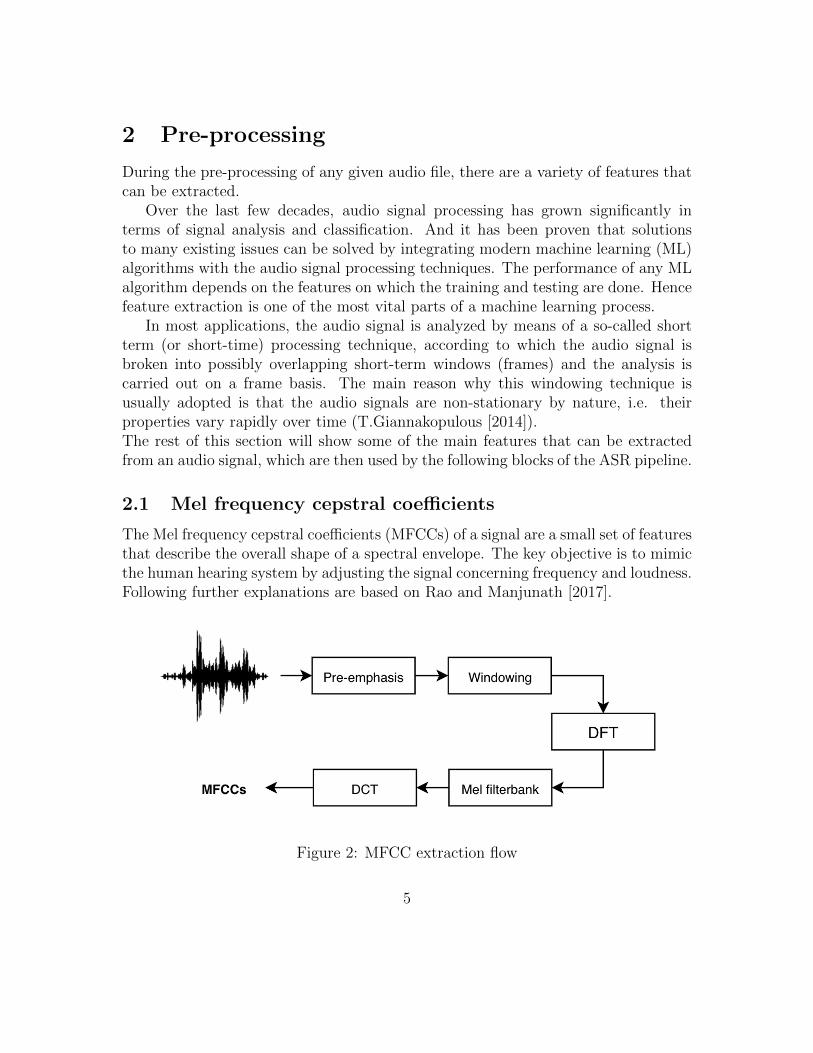
2.1 Mel frequency cepstral coefficients

The Mel frequency cepstral coefficients (MFCCs) of a signal are a small set of featuresthat describe the overall shape of a spectral envelope. The key objective is to mimicthe human hearing system by adjusting the signal concerning frequency and loudness.Following further explanations are based on Rao and Manjunath [2017].

Figure 2: MFCC extraction flow

5

1. Pre-emphasis: Pre-emphasis has the purpose to boost high frequencies tomake information in higher formants more available to the acoustic model. Forvoiced segments like vowels, there is more energy at lower frequencies than athigher frequency levels.

The pre-emphasis filter can be applied to a signal by using the following equa-tion:

y(t) = x(t)− αx(t− 1)

where α is the filter coefficient with typical values between 0.9 and 1

Figure 3: Signal with pre-emphasis filter (α = 0.97)

2. Windowing: After pre-emphasis, the signal is split into short time-frames.The reasoning behind this is that the frequencies in the signal are slowly time-varying. Therefore, the speech analysis must be carried out on short segmentsacross which the speech signal is assumed to be stationary. The typical frameis between 20ms and 30ms, with an overlap of 1

3of the frame size.

After slicing the signal into frames, a window function such as the Hanningwindow is applied to each frame.

The function for the Hanning window (α = 0.5) is:

w(n) = (1− α)− α cos( 2πn

L− 1)

6

Figure 4: Effect of windowing (time domain)

where L is the window size, and n the sliced frame.

Applying a windowing function is mainly to smooth the edges to account for thedrop off in amplitude, that else will create a lot of noise in the high-frequencyspectrum.

3. Discrete Fourier Transform (DFT): When sound is recorded we only cap-ture the resultant amplitudes of those multiple waves. Fourier Transform isa mathematical concept that can decompose a signal into its constituent fre-quencies, together with their magnitude.

X(k) = x(n)N−1∑n=0

x(n)e−i 2πN

kn

7

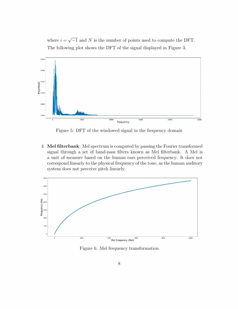
where i =√−1 and N is the number of points used to compute the DFT.

The following plot shows the DFT of the signal displayed in Figure 3.

Figure 5: DFT of the windowed signal in the frequency domain

4. Mel filterbank: Mel spectrum is computed by passing the Fourier transformedsignal through a set of band-pass filters known as Mel filterbank. A Mel isa unit of measure based on the human ears perceived frequency. It does notcorrespond linearly to the physical frequency of the tone, as the human auditorysystem does not perceive pitch linearly.

Figure 6: Mel frequency transformation

8

The Mel scale is approximately linear below 1 kHz and a logarithmic above 1kHz. The approximation of Mel from physical frequency can be expressed as

fMel = 2595 log10(1 +f

700)

where f is the physical frequency in Hz, and fMel denotes the perceived fre-quency.

The final conversion of the DFT to the Mel-scale power spectrum is done byapplying triangular Mel-scale filter banks to the squared output of the DFT ateach frequency x(k)2.

Figure 7: Mel filterbank

The output for each Mel-scale power spectrum slot represents the energy froma number of frequency bands that it covers.

s(m) =N−1∑k=0

Wm(k) |X(k)2|

where k is the DFT bin number and m the Mel filterbank number. Wm(k)is the weight given to the kth energy spectrum bin, contributing to the mth

output band.

9

Figure 8: Mel filterbank

5. Discrete Cosine Transform (DCT) It turns out that filter bank coefficientscomputed in the previous step are highly correlated, which could be problematicfor some machine learning algorithms. Therefore, DCT is used to decorrelatethe filter bank coefficients and yield a compressed representation of the filterbanks. Before computing DCT, the Mel spectrum is usually represented on alog scale. For most ASR applications, the resulting cepstral coefficients 2-13are retained and the rest are discarded. MFCC is equivalent to the inverseDFT and calculated as

c(n) =M−1∑m=0

log10 s(m) cos

(π n (m− 0.5)

M

)

Figure 9: Visualization of the 12 Mel-frequency cepstral coefficients

10

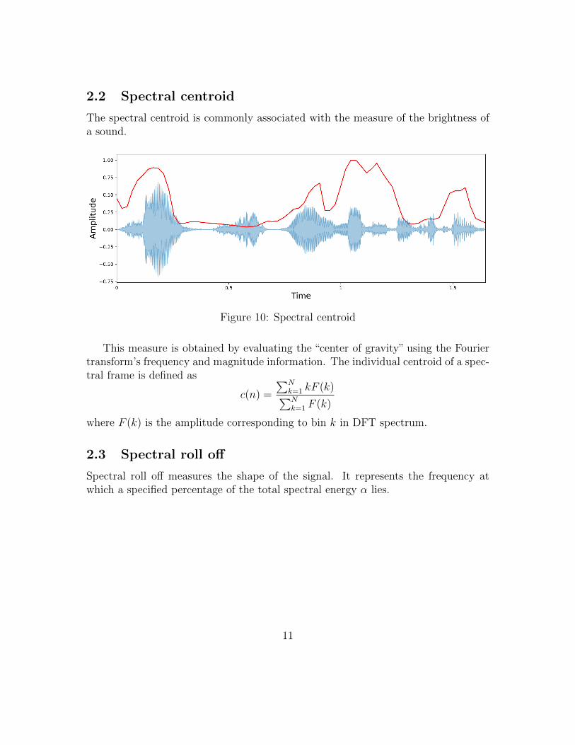
2.2 Spectral centroid

The spectral centroid is commonly associated with the measure of the brightness ofa sound.

Figure 10: Spectral centroid

This measure is obtained by evaluating the “center of gravity” using the Fouriertransform’s frequency and magnitude information. The individual centroid of a spec-tral frame is defined as

c(n) =

∑Nk=1 kF (k)∑Nk=1 F (k)

where F (k) is the amplitude corresponding to bin k in DFT spectrum.

2.3 Spectral roll off

Spectral roll off measures the shape of the signal. It represents the frequency atwhich a specified percentage of the total spectral energy α lies.

11

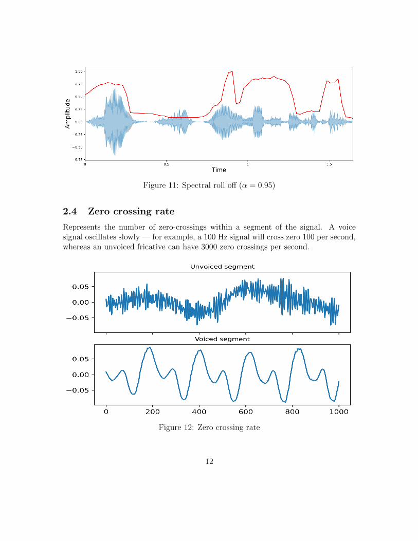
Figure 11: Spectral roll off (α = 0.95)

2.4 Zero crossing rate

Represents the number of zero-crossings within a segment of the signal. A voicesignal oscillates slowly — for example, a 100 Hz signal will cross zero 100 per second,whereas an unvoiced fricative can have 3000 zero crossings per second.

Figure 12: Zero crossing rate

12

3 Voice activity detection

Voice activity detection (VAD) is the task of detecting speech regions in a givenaudio stream or recording. Most of the algorithms proposed for VAD can be dividedinto two processing stages:

• First, features are extracted from the noisy speech signal to achieve a repre-sentation that discriminates between speech and noise.

• In a second stage, a detection scheme is applied to the features resulting in thefinal decision.

3.1 Related literature

Numerous studies have addressed the problem of VAD in the literature. Earlyworks focused on energy-based features, possibly combined with the zero-crossingrate (ZCR) (B. Kotnik [2001], F. Lamel [1981]). These features are however highlyaffected in the presence of additive noise. Therefore, various other features suchas Mel-Frequency Cepstral Coefficients (MFCCs) (T. Kristjansson [2005]) have beenproposed. Some other methods are based on a statistical model of the DiscreteFourier Transform (DFT) coefficients (J. Sohn [1999], J. Ramirez [2005]).

Finally, some studies have addressed the use of a combination of multiple features.These works differ by the way the features are combined: using a linear combinationwhere the weights are trained via a minimum classification error in (Y. Kida [2005]),a linear or a kernel discriminant analysis in (S. Soleimani [2008]) or a principal com-ponent analysis in (S.O. Sadjadi [2013]).

The resulting acoustic information is then generally the input of a statisticalmodel whose goal is to draw a decision about the presence or not of speech. Proposedapproaches differ in whether they use a supervised framework or not.

For modeling, several approaches have been used: Gaussian Mixture Models(GMM, Ng et al. [2012]), Hidden Markov Models (HMM, Harsha [2004]) which havemore and more been replaced by Neural Network approaches with tasks rangingfrom VAD in a multi-room domestic environment (Ferroni et al. [2015]) to VAD forsmartphone applications (Sehgal and Kehtarnavaz [2018]).

Following are some of the more recent approaches which have been developed toopen-source toolkits:

• Pyannote audio (Bredin et al. [2020]), having a Neural Network as underlyingdiscrimination model.

13

• Ina speech segmenter (Doukhan et al. [2018]), as a CNN-based audio segmen-tation toolkit.

• WebrtcVAD (Google [2011]), with a Gaussian Mixture Model (GMM) ap-proach.

The next section provides an overview of each module, together with its perfor-mance to Voice Activity Detection.

3.2 Evaluation metrics

Evaluations were made on all datasets stated in (1.1), with the following evaluationmetrics:

Detection accuracy, where the positive class is considered as speech region. Gapsin the inputs are considered as the negative class (e.g. non-speech regions).

Detection error rate, where false alarm is the duration of non-speech incor-rectly classified as speech, missed detection is the duration of speech incorrectlyclassified as non-speech, and total is the total duration of speech in the reference.

detection error rate =false alarm+missed detection

total

Detection precision, computed as tptp+fp

, where tp is the duration of true positive

(e.g. speech classified as speech), and fp is the duration of false positive (e.g. non-speech classified as speech).

Detection recall, computed as tptp+fn

, where tp is the duration of true positive (e.g.

speech classified as speech), and fn is the duration of false negative (e.g. speechclassified as non-speech).

To ensure reproducibility, pyannote.metrics (Bredin [2017]) is used as an evaluationprotocol, which has a large set of evaluation metrics for diagnostic purposes of allmodules of a typical ASR pipeline.

14

3.3 Pyannote audio

Pyannote is Based on the PyTorch machine learning framework (Paszke et al. [2017]),it provides a set of trainable end-to-end neural building blocks that can be com-bined and jointly optimized to build pipelines for different ASR tasks. It comeswith pre-trained models covering a wide range of domains including VAD. For thenext evaluations, the model sad ami is used, which can be loaded via torch.hub(https://pytorch.org/docs/stable/hub.html) with the repo name pyannote/pyannote−audio.

To show the evaluation process, Figure 13 shows the ground truth time windowof a sample audio recording, picked from the AMI dataset.

Figure 13: Ground truth timeline

After processing the raw audio signal with the pre-trained model, speaker activa-tion scores are returned which represent the models predictions on the given timeline.

Figure 14: Speaker activation scores

This scores are then binarized based on a threshold to represent the speech andnon-speech regions.

Figure 15: Speaker activation scores (Pyannote)

Features usedThe features used for training the bidirectional LSTMs are SincNet learnable features

15

https://pytorch.org/docs/stable/hub.html

(Ravanelli and Bengio [2018]), together with MFCCs (2.1).

ResultsThe following table shows the results of the preceding evaluation process, applied toall four datasets (resulting in a total of 2131 individual audio files). The scores areaveraged over all corpora of the individual segments.

AMI Ava Arabic ICSI Mean

Accuracy 0.930 0.790 0.821 0.715 0.810Error rate 0.087 0.394 0.180 0.320 0.245Precision 0.976 0.827 0.998 0.981 0.946Recall 0.937 0.770 0.821 0.693 0.805

Table 1: Pyannote VAD performance metrics

As shows, very good results are achieved in terms of precision and accuracy, lowerperformance for corpora which higher noise content (AVA, ICSI).

3.4 Ina speech segmenter

Ina speech segmenter is a CNN-based audio segmentation toolkit, designed for con-ducting gender equality studies. It splits audio signals into homogeneous zones ofspeech, music and noise.Providing, in addition to VAD, the possibility to tag signals by speaker gender (maleor female). In the experiments, zones corresponding to speech over music or speechover noise are tagged as speech.

For a visual comparison, the figure below shows the binarized speaker activationscores over the same sample segment picked in (3.3), where small differences can beseen between t = 640 and t = 660.

Figure 16: Speaker activation scores (Ina)

16

Features usedThe system uses log-mel filterbank features (2.1), together with 4 convolutional and4 dense layers .

ResultsThe following table shows the results, applied to all four datasets (resulting in atotal of 2131 individual audio files). The scores are averaged over all corpora of theindividual segments.



Table 2: Ina VAD performance metrics

Here the main improvement with regard to the previous method is seen in theArabic dataset (Aranorm [2020]), having an increased accuracy of almost 10%.

3.5 Webrtc VAD

Webrtc is a project providing real-time communication capabilities for many differ-ent applications. The project is actively maintained by the Google Webrtc Team.It uses a Gaussian Mixture Model (GMM), which is typically much more effectivethan a simple energy-threshold detector, especially in a situation with dynamic lev-els and types of background noise. The only parameter that can be chosen forthis method is the aggressiveness parameter with integer values between 0 (leastaggressive) to 3 (most aggressive), which should reflect the threshold by which voice-activity is done. For the experiments the parameter is set at 2 and kept fix acrossall evaluations.

To evaluate successive audio frames, a padded sliding window algorithm is used.When more than 90% of the frames in the window are voiced (as reported by thedetector), the collector triggers and begins yielding audio frames. Then the collec-tor waits until 90% of the frames in the window are unvoiced to de trigger. Thewindow is padded at the front and back to provide a small amount of silence or thebeginnings/endings of speech around the voiced frames.

17

Figure 17: Speaker activation scores (WebRTC)

Features usedWebRTC VAD only accepts 16-bit mono Pulse-code modulation (PCM) signals, sam-pled at 8000, 16000, 32000 or 48000 Hz. To this purpose, the audio signal is convertedto PCM with a frame-length of 20ms before being fed to the discriminator model.

ResultsThe following table shows the results of experiments, applied to all four datasets(resulting in a total of 2131 individual audio files). The scores are averaged over allcorpora of the individual segments.



Table 3: WebrtcVAD performance metrics

Interesting to note here is that even though GMM’s should be able to handledynamic levels and types of noise, WebRtc performs very badly on the AVA-speech(Speech [2018]) dataset which contains high amounts of background noises.

3.6 Ensemble

As the last step of the VAD evaluation, ensemble predictors are created as an ex-tension of the tested toolkits. To create the ensemble, overlapping intervals arecalculated on a sliding window of 0.1s between the predictions of all three methods.Then, the experiments are extended on the following ensembles:

• Ensemble of two: Representing the combination of predictors where at least 2prediction-intervals are intersecting.

• Ensemble of three: Representing the combination of predictors where all of the3 prediction-intervals are intersecting.

18

The following two tables show the results of applying the ensemble predictors toall four datasets (resulting in a total of 2131 individual audio files). The scores areaveraged over all corpora of the individual segments.



Table 4: Ensemble of 2 predictors - performance metrics



Table 5: Ensemble of 3 predictors - performance metrics

Here to see is that both methods show improvement in terms of accuracy over theindividual methods. While the ensemble of 2 predictors are best regarding precision,for the application of VAD the combination of 3 predictors seems to be the go-tomethod, with a recall (correctly classifying the non-speech segments as non-speech)of 0.924 .

19

3.7 Comparing Results

This section shows more details, comparing the detection specifics of every toolkiton a sample corpora, together with a summarizing table with the aggregated perfor-mance on all evaluations made.

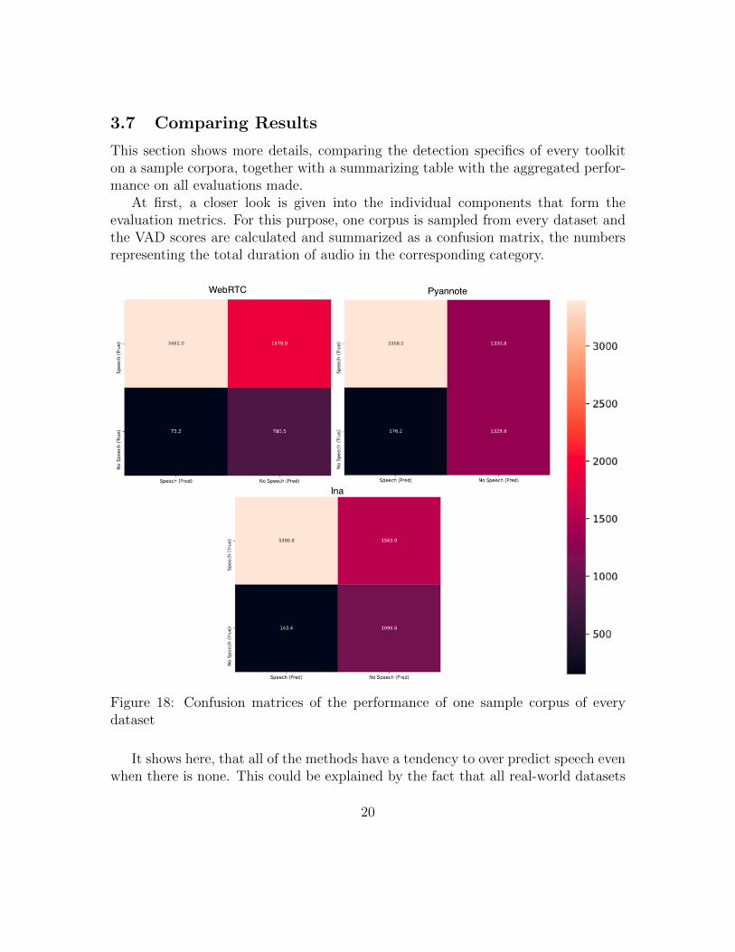
At first, a closer look is given into the individual components that form theevaluation metrics. For this purpose, one corpus is sampled from every dataset andthe VAD scores are calculated and summarized as a confusion matrix, the numbersrepresenting the total duration of audio in the corresponding category.

Figure 18: Confusion matrices of the performance of one sample corpus of everydataset

It shows here, that all of the methods have a tendency to over predict speech evenwhen there is none. This could be explained by the fact that all real-world datasets

20

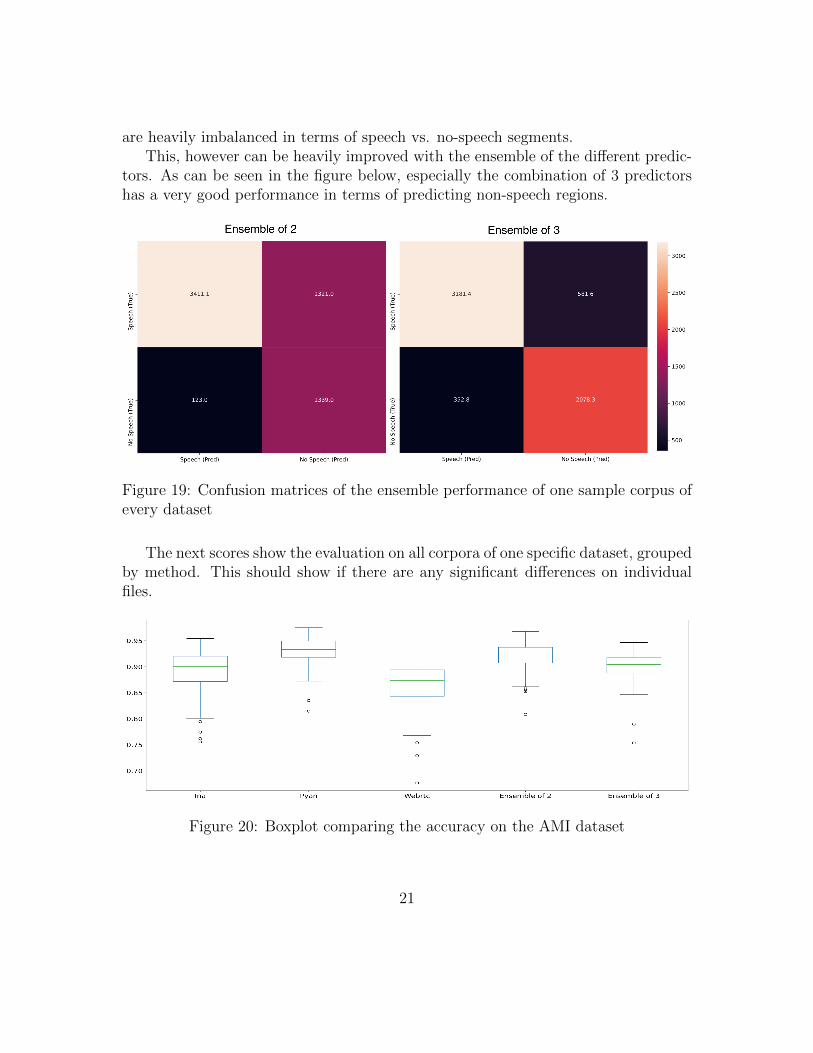
are heavily imbalanced in terms of speech vs. no-speech segments.This, however can be heavily improved with the ensemble of the different predic-

tors. As can be seen in the figure below, especially the combination of 3 predictorshas a very good performance in terms of predicting non-speech regions.

Figure 19: Confusion matrices of the ensemble performance of one sample corpus ofevery dataset

The next scores show the evaluation on all corpora of one specific dataset, groupedby method. This should show if there are any significant differences on individualfiles.

Figure 20: Boxplot comparing the accuracy on the AMI dataset

21

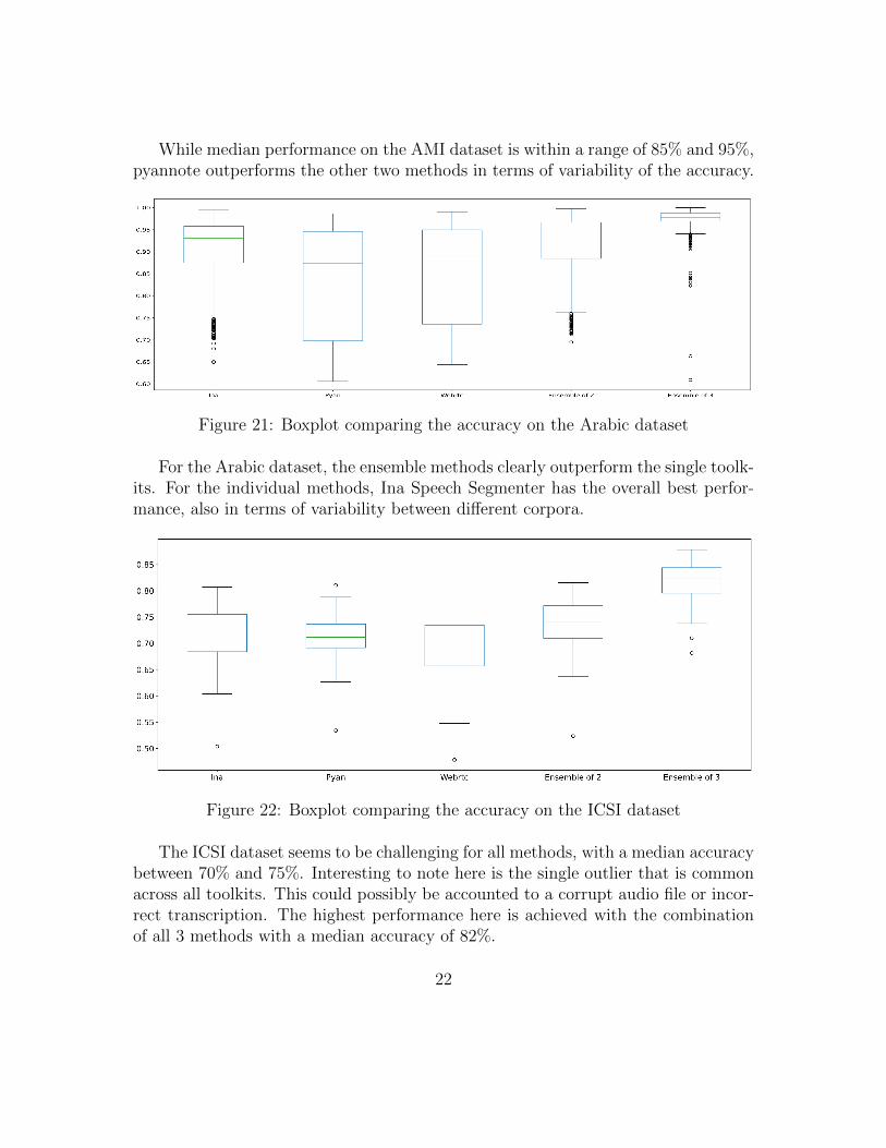
While median performance on the AMI dataset is within a range of 85% and 95%,pyannote outperforms the other two methods in terms of variability of the accuracy.

Figure 21: Boxplot comparing the accuracy on the Arabic dataset

For the Arabic dataset, the ensemble methods clearly outperform the single toolk-its. For the individual methods, Ina Speech Segmenter has the overall best perfor-mance, also in terms of variability between different corpora.

Figure 22: Boxplot comparing the accuracy on the ICSI dataset

The ICSI dataset seems to be challenging for all methods, with a median accuracybetween 70% and 75%. Interesting to note here is the single outlier that is commonacross all toolkits. This could possibly be accounted to a corrupt audio file or incor-rect transcription. The highest performance here is achieved with the combinationof all 3 methods with a median accuracy of 82%.

22

Figure 23: Boxplot comparing the accuracy on the AVA dataset

On the AVA dataset, performance is similar for Ina Speech Segmenter and Pyan-note, the latter having a IQR between 65% and 90%. WebRTC clearly having prob-lems with this ”noisy” dataset, with an outlier at 15% accuracy.

Finally, the following table shows the mean performance of every evaluated mod-ule over all datasets:

Pyannote Ina Webrtc Ensemble 2 Ensemble 3


Table 6: Mean performance on all evaluated datasets

To conclude here is that especially for Voice Activity Detection the ensemblemethods are to be favoured over the individual toolkits.

For a practical viewpoint of the discussed methods, there are two other importantthings to compare. First, the computing time that a method takes to predict thespeech and non-speech sections and secondly the possible consideration of a thresh-old that serves as a lower boundary for regions to be not considered if they fall belowit.

23

For the computing time, this can vary substantially for the evaluated toolkits.The table below shows the mean elapsed time (in seconds) for predicting one audiofile of the corpora.

AMI Ava Arabic ICSI

Pyannote 509.69 1039.95 0.845 1725.53Ina 49.38 26.56 0.34 93.26Webrtc 0.89 0.95 0.02 1.58

Table 7: Computation time

As expected, for Neural-Network-based models it takes substantially more timeto compute the predictions than for the GMM-based Webrtc toolkit.

To evaluate the effectiveness of limiting the considered segments to a certainthreshold, the experiments of the beginning of this section are repeated on one samplecorpus from every dataset with the following schema applied to both the transcribedground truth, as well as the predictions:

For every label, yt, t = {1, 2, ...T} the duration of the segment to the correspond-ing label is checked, for both speech-segments, as well as non-speech segments. If theduration of the segment falls below a threshold |t − t−1| ≤ δ, δ = {0.2s, 0.5s}, thenthe current label is extended by the preceding one, potentially overriding the classattribution. The described process is depicted in Figure 24, showing the timelinebefore and after applying the threshold.

Figure 24: Annotation after smoothing with δ = 0.5

Before applying this threshold approach to the sampled datasets, the amount ofaffected (non-speech) segments that are calculated, together with their distribution.

24

AMI Ava Arabic ICSI

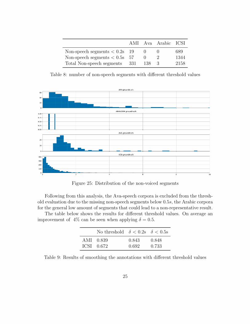
Non-speech segments < 0.2s 19 0 0 689Non-speech segments < 0.5s 57 0 2 1344Total Non-speech segments 331 138 3 2158

Table 8: number of non-speech segments with different threshold values

Figure 25: Distribution of the non-voiced segments

Following from this analysis, the Ava-speech corpora is excluded from the thresh-old evaluation due to the missing non-speech segments below 0.5s, the Arabic corporafor the general low amount of segments that could lead to a non-representative result.

The table below shows the results for different threshold values. On average animprovement of 4% can be seen when applying δ = 0.5.

No threshold δ < 0.2s δ < 0.5s

AMI 0.839 0.843 0.848ICSI 0.672 0.692 0.733

Table 9: Results of smoothing the annotations with different threshold values

25

4 Overlapping speech detection

The presence of overlapped, or parallel, speech in meetings is a common occurrenceand a natural consequence of the spontaneous multiparty conversations which arisewithin meetings. This speech presents a significant challenge to ASR systems thatprocess audio data from meetings. In the case of speaker diarization, current state-of-the-art systems assign speech segments to only one speaker, thus incurring missedspeech errors in regions where more than one speaker is active. Studies have shownthat the presence of overlapping speech may increase diarization error rates up to27% (Ryanta et al. [2018]). To address this, one may either separate the speakersin an overlapped speech segment or completely exclude these segments in the dataprocessing altogether. Regardless of the approach, overlapping speech segments mustfirst be detected in order to be addressed; this task is called overlapping speechdetection.

4.1 Related Literature

There are numerous existing studies for overlapping speech detection. Several featureadditions are proposed: Zelenak and Hernando [2011] Shows the potential of com-plementing the overlap detection system, based on short-term spectral parameters,with a set of prosody-based long-term features. Additional higher-level informationfrom the structure of a conversation such as silence and speaker change statistics areproposed by Yella and Bourlard [2014] to improve the feature-based classifier of over-lapping and single-speaker speech classes. The silence and speaker change statisticsare computed over a long-term window (around 3-4 seconds) and are used to predictthe probability of overlap in the window. These estimates are then incorporated asprior probabilities of the classes.

In Geiger et al. [2013], the central idea is to use language models to detectbackchannel words and other language characteristics that typify instances of overlap.The language models are then used within a HMM framework to assign scores to eachword in a dictionary and thus to estimate the probability that the linguistic contentreflects overlapping speech. For the domain of driver assessment in vehicle activesafety systems, Shokouhi et al. [2013] show increased accuracy by the use of spectralharmonicity and envelope features to represent overlapped and single-speaker speechusing Gaussian mixture models (GMM).

More recently, approaches such as Sajjan et al. [2018] show that Neural Networkssuch as LSTMs are effective in overlap detection, by outperforming existing resultsmade GMMs with the use of spectrograms instead of specialized handcrafted features.

26

Despite the variety of research in the field of overlapping speech detection, theopen-source toolkits are very limited with pyannote (Bredin et al. [2020]) being themain API providing overlapping speech detection capabilities. For the purpose ofevaluation the next section will show the performance of the existing toolkit, com-pared with different types of neural networks.

4.2 Evaluation metrics

For overlapping speech detection, the same metrics are used as in 3.2, where thepositive class is considered as non-parallel speech (single speaker or no speech), over-lapping speech is considered as the negative class. To calculate the overlaps, theannotation is analyzed on a sliding window of 0.1s using the labeling principle withyt = 1 if there is zero or one speaker at time step t and yt = 0 if there are twospeakers or more.

The process is depicted in the following figure, showing the original timeline andthe timeline considering only overlapping segments:

Figure 26: Timeline before and after calculating the overlapping segments

These overlaps are calculated as prerequisite for every corpora of the AMI and ICSIdataset and used in the upcoming section for the performance evaluation of the statedmethods.

27

4.3 Pyannote audio

As one of the inbuilt blocks of pyannote, the evaluation process is similar for the over-lapping speech detection as it is for voice activity detection. Predictions are returnedas probabilities which are then binarized to represent the two classes: overlappingspeech and non-overlapping speech (silence included). For the evaluated datasets,the following performance is achieved:

AMI ICSI

Accuracy 0.931 0.944Error rate 0.586 0.963Precision 0.771 0.560Recall 0.599 0.302

Table 10: Pyannote OVL performance metrics

The metric of interest here is in most of the cases precision (how much of thepredicted overlaps are in fact overlapping speech). Since this is a difficult task Bytaking a closer look it shows that the precision varies quite a lot between differentdatasets, especially within the ICSI corpus.

Figure 27: Pyannote precision values over the two corpora

28

4.4 Neural Networks

As the last approach, different types of Neural Networks are trained to have a base-line to compare with pyannote on the task of Overlapping speech detection. Theconsidered network structures are: Dense and LSTM. As input for the network, 27numerical features aligned with the description in section 2 are extracted from theaudio signal over a window of 0.1s. In detail, those are root-mean-square, chroma,spectral centroid, spectral bandwidth, min and max spectral roll-off, zero-crossingrate, and 20 mfccs.

The AMI and ICSI corpora are split into a training and test part with proportion7:3, resulting in a total of 172 training datasets and 73 test datasets. For the hyper-parameters, a grid-search is performed on the training set, resulting in the followingparameters for each network:

Dense LSTM

Activation tanh reluBatch size 40 60Dropout rate 0.2 0.4Kernel initialization uniform glorot uniformLearning rate 0.01 0.001

Table 11: Network parameters

Regarding layer structure, 4 layers are used for each network with 256 Neuronsfor the hidden layers and a binary dense layer as output layer. For the evaluateddatasets, the following performance is achieved:

Dense Network

AMI ICSI


Table 12: Dense Network precision values over the two corpora

29

LSTM Network

AMI ICSI


Table 13: LSTM network OVL performance metrics

Both methods show a clear decrease in detecting overlapping speech in comparisonto the pyannote toolkit. In particular for training an own network the imbalancebetween the positive and negative class is a difficult challenge to handle and couldbe a prospect for further research.

5 Conclusion

This research presented an overview of the available toolkits for Voice Activity De-tection and Overlapping Speech Detection, together with some of the main featuresthat are extracted from the raw audio signal and used within the different models.

Evaluating the best-performing methods, the ensemble method of combining 3different classifiers has proven the most successful for VAD, with an overall accuracyof 87% and a recall correctly classifying the non-speech segments as non-speech) of0.924.

For Overlapping Speech Detection, pyannote shows already promising results witha precision rate of 66% over basic Neural Networks, although further research has tobe made on other types of methods to get a representative comparison.

30

References

AMI, 2006. Ami meeting corpus. URL: http://groups.inf.ed.ac.uk/ami/

download/.

Aranorm, 2020. Arabic speech corpus. URL: http://en.arabicspeechcorpus.

com/.

B. Kotnik, Z. Kacic, B.H., 2001. A multiconditional robust front-end feature ex-traction with a noise reduction procedure based on improved spectral subtractionalgorithm. Proc. 7th Europseech .

Bredin, H., 2017. pyannote.metrics: a toolkit for reproducible evaluation, diagnosticand error analysis of speaker diarization systems. URL: https://github.com/pyannote/pyannote-metrics.

Bredin, H., Yin, R., Coria, J.M., Gelly, G., Korshunov, P., Lavechin, M., Fustes, D.,Titeux, H., Bouaziz, W., Gill, M.P., 2020. pyannote.audio: neural building blocksfor speaker diarization. URL: https://github.com/pyannote/pyannote-audio.

Doukhan, D., Lechapt, E., Evrard, M., Carrive, J., 2018. Ina’s mirex 2018 music andspeech detection system, in: Music Information Retrieval Evaluation eXchange(MIREX 2018).

F. Lamel, R. Rabiner, E.R.G.W., 1981. An improved endpoint detector for isolatedword recognition. IEEE Trans .

Ferroni, G., Bonfigli, R., Principi, E., Squartini, S., Piazza, F., 2015. A deep neuralnetwork approach for voice activity detection in multi-room domestic scenarios,in: 2015 International Joint Conference on Neural Networks (IJCNN), pp. 1–8.

Geiger, J., Eyben, F., Evans, N., Schuller, B., Rigoll, G., 2013. Using linguisticinformation to detect overlapping speech.

Google, 2011. Webrtcvad. URL: https://webrtc.org/.

Harsha, B., 2004. A noise robust speech activity detection algorithm, pp. 322 – 325.doi:10.1109/ISIMP.2004.1434065.

ICSI, 2003. Icsi meeting corpus. URL: http://groups.inf.ed.ac.uk/ami/icsi/download/.

31

http://groups.inf.ed.ac.uk/ami/download/

http://groups.inf.ed.ac.uk/ami/download/

http://en.arabicspeechcorpus.com/

http://en.arabicspeechcorpus.com/

https://github.com/pyannote/pyannote-metrics

https://github.com/pyannote/pyannote-metrics

https://github.com/pyannote/pyannote-audio

https://webrtc.org/

http://dx.doi.org/10.1109/ISIMP.2004.1434065

http://groups.inf.ed.ac.uk/ami/icsi/download/

http://groups.inf.ed.ac.uk/ami/icsi/download/

J. Ramirez, J. Segura, M.B.L.G.A.R., 2005. Statistical voice activity detection usinga multiple observation likelihood ratio test. IEEE Signal Proc. Letters, vol. 12 .

J. Sohn, N. Kim, W.S., 1999. A statistical model-based voice activity detection.IEEE Sig. Pro. Letters, vol. 6 .

ldc, 2003. rttm format. URL: https://catalog.ldc.upenn.edu/docs/

LDC2004T12/RTTM-format-v13.pdf.

Ng, T., Zhang, B., Nguyen, L., Matsoukas, S., Zhou, X., Mesgarani, N., Vesel, K.,Matejka, P., 2012. Developing a speech activity detection systemforthe darpa ratsprogram. In Proceedings of the 13th Annual Conference of the International Speech(InterSpeech) .

Paszke, A., Gross, S., Chintala, S., Chanan, G., Yang, E., DeVito, Z., Lin, Z.,Desmaison, A., Antiga, L., Lerer, A., 2017. Automatic differentiation in pytorch,in: NIPS-W.

Rao, K., Manjunath, K., 2017. Speech Recognition Using Articulatory and ExcitationSource Features. Springer.

Ravanelli, M., Bengio, Y., 2018. Speaker recognition from raw waveform with sincnet.arXiv:1808.00158.

Ryanta, N., Bergelson, E., Church, K., Cristia, A., Du, J., Ganapathy, S., Khudan-pur, S., Kowalski, D., Krishnamoorthy, M., Kulshreshta, R., Liberman, M., Lu,Y.D., Maciejewski, M., Metze, F., Profant, J., Sun, L., Tsao, Y., Yu, Z., 2018.Enhancement and analysis of conversational speech: Jsalt 2017, pp. 5154–5158.doi:10.1109/ICASSP.2018.8462468.

S. Soleimani, S.A., 2008. Voice activity detection based on combination of multiplefeatures using linear/kernel discriminant analyses. Proc. Information and Com-munication Technologies: From Theory to Applications .

Sajjan, N., Ganesh, S., Sharma, N., Ganapathy, S., Ryant, N., 2018. Leveraginglstm models for overlap detection in multi-party meetings, pp. 5249–5253. doi:10.1109/ICASSP.2018.8462548.

Sehgal, A., Kehtarnavaz, N., 2018. A convolutional neural network smartphone appfor real-time voice activity detection. IEEE Access 6, 9017–9026.

32

https://catalog.ldc.upenn.edu/docs/LDC2004T12/RTTM-format-v13.pdf

https://catalog.ldc.upenn.edu/docs/LDC2004T12/RTTM-format-v13.pdf

http://arxiv.org/abs/1808.00158

http://dx.doi.org/10.1109/ICASSP.2018.8462468



Shokouhi, N., Sathyanarayana, A., Sadjadi, S., Hansen, J., 2013. Overlapped-speechdetection with applications to driver assessment for in-vehicle active safety systems.doi:10.1109/ICASSP.2013.6638174.

S.O. Sadjadi, J.H., 2013. Unsupervised speech activity detection using voicing mea-sures and perceptual spectral flux. IEEE Sig. Pro. Letters,vol. 20 .

Speech, A., 2018. Ava speech. URL: http://research.google.com/ava/.

T. Kristjansson, S. Deligne, P.O., 2005. Voicing features for robust speech detection.Proc. Interspeech .

T.Giannakopulous, A., 2014. Introduction to Audio Analysis. Elsevier.

Y. Kida, T.K., 2005. Voice activity detection based on optimally weighted combina-tion of multiple features. Proc. Interspeech .

Yella, S.H., Bourlard, H., 2014. Overlapping speech detection using long-termconversational features for speaker diarization in meeting room conversations.IEEE/ACM Transactions on Audio, Speech, and Language Processing 22, 1688–1700.

Zelenak, M., Hernando, J., 2011. The detection of overlapping speech with prosodicfeatures for speaker diarization., pp. 1041–1044.

33


http://research.google.com/ava/

List of Figures

1 Speech recognition pipeline . . . . . . . . . . . . . . . . . . . . . . . . 22 MFCC extraction flow . . . . . . . . . . . . . . . . . . . . . . . . . . 53 Signal with pre-emphasis filter (α = 0.97) . . . . . . . . . . . . . . . . 64 Effect of windowing (time domain) . . . . . . . . . . . . . . . . . . . 75 DFT of the windowed signal in the frequency domain . . . . . . . . . 86 Mel frequency transformation . . . . . . . . . . . . . . . . . . . . . . 87 Mel filterbank . . . . . . . . . . . . . . . . . . . . . . . . . . . . . . . 98 Mel filterbank . . . . . . . . . . . . . . . . . . . . . . . . . . . . . . . 109 Visualization of the 12 Mel-frequency cepstral coefficients . . . . . . . 1010 Spectral centroid . . . . . . . . . . . . . . . . . . . . . . . . . . . . . 1111 Spectral roll off (α = 0.95) . . . . . . . . . . . . . . . . . . . . . . . . 1212 Zero crossing rate . . . . . . . . . . . . . . . . . . . . . . . . . . . . . 1213 Ground truth timeline . . . . . . . . . . . . . . . . . . . . . . . . . . 1514 Speaker activation scores . . . . . . . . . . . . . . . . . . . . . . . . . 1515 Speaker activation scores (Pyannote) . . . . . . . . . . . . . . . . . . 1516 Speaker activation scores (Ina) . . . . . . . . . . . . . . . . . . . . . . 1617 Speaker activation scores (WebRTC) . . . . . . . . . . . . . . . . . . 1818 Confusion matrices of the performance of one sample corpus of every

dataset . . . . . . . . . . . . . . . . . . . . . . . . . . . . . . . . . . . 2019 Confusion matrices of the ensemble performance of one sample corpus

of every dataset . . . . . . . . . . . . . . . . . . . . . . . . . . . . . . 2120 Boxplot comparing the accuracy on the AMI dataset . . . . . . . . . 2121 Boxplot comparing the accuracy on the Arabic dataset . . . . . . . . 2222 Boxplot comparing the accuracy on the ICSI dataset . . . . . . . . . 2223 Boxplot comparing the accuracy on the AVA dataset . . . . . . . . . 2324 Annotation after smoothing with δ = 0.5 . . . . . . . . . . . . . . . . 2425 Distribution of the non-voiced segments . . . . . . . . . . . . . . . . . 2526 Timeline before and after calculating the overlapping segments . . . . 2727 Pyannote precision values over the two corpora . . . . . . . . . . . . 28

34

List of Tables

1 Pyannote VAD performance metrics . . . . . . . . . . . . . . . . . . 162 Ina VAD performance metrics . . . . . . . . . . . . . . . . . . . . . . 173 WebrtcVAD performance metrics . . . . . . . . . . . . . . . . . . . . 184 Ensemble of 2 predictors - performance metrics . . . . . . . . . . . . 195 Ensemble of 3 predictors - performance metrics . . . . . . . . . . . . 196 Mean performance on all evaluated datasets . . . . . . . . . . . . . . 237 Computation time . . . . . . . . . . . . . . . . . . . . . . . . . . . . 248 number of non-speech segments with different threshold values . . . . 259 Results of smoothing the annotations with different threshold values . 2510 Pyannote OVL performance metrics . . . . . . . . . . . . . . . . . . 2811 Network parameters . . . . . . . . . . . . . . . . . . . . . . . . . . . 2912 Dense Network precision values over the two corpora . . . . . . . . . 2913 LSTM network OVL performance metrics . . . . . . . . . . . . . . . 30

35

a comparative analysis of the speech detection pipeline

Documents