a comparative anatomy of credit risk modelsrvicente/risco/gordy.pdf · with comparative analyses....

A comparative anatomy of credit risk models

Michael B. Gordy *

Board of Governors of the Federal Reserve System, Division of Research and Statistics,

Washington, DC 20551, USA

Abstract

Within the past two years, important advances have been made in modeling credit risk

at the portfolio level. Practitioners and policy makers have invested in implementing and

exploring a variety of new models individually. Less progress has been made, however,

with comparative analyses. Direct comparison often is not straightforward, because the

di�erent models may be presented within rather di�erent mathematical frameworks. This

paper o�ers a comparative anatomy of two especially in¯uential benchmarks for credit

risk models, the RiskMetrics Group's CreditMetrics and Credit Suisse Financial Prod-

uct's CreditRisk�. We show that, despite di�erences on the surface, the underlying

mathematical structures are similar. The structural parallels provide intuition for the

relationship between the two models and allow us to describe quite precisely where the

models di�er in functional form, distributional assumptions, and reliance on approxi-

mation formulae. We then design simulation exercises which evaluate the e�ect of each of

these di�erences individually. Ó 2000 Elsevier Science B.V. All rights reserved.

JEL classi®cation: G31; C15; G11

Keywords: Credit risk; Comparative analysis; Financial products

1. Introduction

Over the past decade, ®nancial institutions have developed and implementeda variety of sophisticated models of value-at-risk for market risk in tradingportfolios. These models have gained acceptance not only among senior bank

Journal of Banking & Finance 24 (2000) 119±149

www.elsevier.com/locate/econbase

* Corresponding author. Tel.: +1-202-452-3705; fax: +1-202-452-5295.

E-mail address: [email protected] (M.B. Gordy).

0378-4266/00/$ - see front matter Ó 2000 Elsevier Science B.V. All rights reserved.

PII: S 0 3 7 8 - 4 2 6 6 ( 9 9 ) 0 0 0 5 4 - 0

managers, but also in amendments to the international bank regulatoryframework. Much more recently, important advances have been made inmodeling credit risk in lending portfolios. The new models are designed toquantify credit risk on a portfolio basis, and thus have application in control ofrisk concentration, evaluation of return on capital at the customer level, andmore active management of credit portfolios. Future generations of today'smodels may one day become the foundation for measurement of regulatorycapital adequacy.

Two of the models, the RiskMetrics Group's CreditMetrics and CreditSuisse Financial Product's CreditRisk�, have been released freely to the publicsince 1997 and have quickly become in¯uential benchmarks. Practitioners andpolicy makers have invested in implementing and exploring each of the modelsindividually, but have made less progress with comparative analyses. The twomodels are intended to measure the same risks, but impose di�erent restrictionsand distributional assumptions, and suggest di�erent techniques for calibrationand solution. Thus, given the same portfolio of credit exposures, the twomodels will, in general, yield di�ering evaluations of credit risk. Determiningwhich features of the models account for di�erences in output would allow us abetter understanding of the sensitivity of the models to the particular as-sumptions they employ.

Direct comparison of the models has so far been limited, in large part, be-cause the two models are presented within rather di�erent mathematicalframeworks. The CreditMetrics model is familiar to econometricians as anordered probit model. Credit events are driven by movements in underlyingunobserved latent variables. The latent variables are assumed to depend onexternal ``risk factors''. Common dependence on the same risk factors gives riseto correlations in credit events across obligors. The CreditRisk� model is basedinstead on insurance industry models of event risk. Instead of a latent variable,each obligor has a default probability. The default probabilities are not con-stant over time, but rather increase or decrease in response to backgroundsystemic factors. To the extent that two obligors are sensitive to the same set ofbackground factors, their default probabilities will move together. These co-movements in probability give rise to correlations in defaults. CreditMetricsand CreditRisk� may serve essentially the same function, but they appear to beconstructed quite di�erently.

This paper o�ers a comparative anatomy of CreditMetrics and CreditRisk�.We show that, despite di�erences on the surface, the underlying probabilisticstructures are similar. Understanding the structural parallels helps to developintuition for the relationship between the two models. More importantly, itallows us to describe quite precisely where the models di�er in functional form,distributional assumptions, and reliance on approximation formulae. We thendesign simulation exercises which evaluate the e�ect of each of these di�erencesindividually.

120 M.B. Gordy / Journal of Banking & Finance 24 (2000) 119±149

We proceed as follows. Section 2 presents a summary of the CreditRisk�

model and introduces a restricted version of CreditMetrics. The restrictions areimposed to facilitate direct comparison of CreditMetrics and CreditRisk�.While some of the richness of the full CreditMetrics implementation is sacri-®ced, the essential mathematical characteristics of the model are preserved. Ourmethod of comparative anatomy is developed in Section 3. We show how therestricted version of CreditMetrics can be run through the mathematical ma-chinery of CreditRisk�, and vice versa.

Comparative simulations are developed in Section 4. Care is taken to con-struct portfolios with quality and loan size distributions similar to real bankportfolios, and to calibrate correlation parameters in the two models in anempirically plausible and mutually consistent manner. The robustness of theconclusions of Section 4 to our methods of portfolio construction and pa-rameter calibration are explored in Section 5. An especially striking result fromthe simulations is the sensitivity of CreditRisk� results to the shape of thedistribution of a systemic risk factor. The reasons for and consequences of thissensitivity are explored in Section 6. We conclude with a summary of the mainresults of the simulations.

2. Summary of the models

This section o�ers an introduction to CreditRisk� and CreditMetrics. Thediscussion of CreditRisk� merely summarizes the derivation presented inCSFP (1997, Appendix A). Our presentation of CreditMetrics sets forth arestricted version of the full model described in the CreditMetrics TechnicalDocument (Gupton et al., 1997). Our choice of notation is intended to facilitatecomparison of the models, and may di�er considerably from what is used in theoriginal manuals.

2.1. Summary of CreditRisk�

CreditRisk� is a model of default risk. Each obligor has only two possibleend-of-period states, default and non-default. In the event of default, the lendersu�ers a loss of ®xed size, this is the lender's exposure to the obligor. Thedistributional assumptions and functional forms imposed by CreditRisk� al-low the distribution of total portfolio losses to be calculated in a convenientanalytic form.

Default correlations in CreditRisk� are assumed to be driven entirely by avector of K ``risk factors'' x � �x1; . . . ; xK�. Conditional on x, defaults ofindividual obligors are assumed to be independently distributed Bernoullidraws. The conditional probability pi�x� of drawing a default for obligor i is afunction of the rating grade f�i� of obligor i, the realization of risk factors x,

M.B. Gordy / Journal of Banking & Finance 24 (2000) 119±149 121

and the vector of ``factor loadings'' �wi1; . . . ;wiK� which measure the sensi-tivity of obligor i to each of the risk factors. CreditRisk� speci®es thisfunction as

pi�x� � �pf�i�XK

k�1

xkwik

!; �1�

where �pf is the unconditional default probability for a grade f obligor, and thex are positive-valued with mean one. The intuition behind this speci®cation isthat the risk factors x serve to ``scale up'' or ``scale down'' the unconditional �pf.A high draw of xk (over one) increases the probability of default for eachobligor in proportion to the obligor's weight wik on that risk factor, a low drawof xk (under one) scales down all default probabilities. The weights wik arerequired to sum to one for each obligor, which guarantees that E�pi�x�� pf�i�.

Rather than calculating the distribution of defaults directly, CreditRisk�

calculates the probability generating function (``pgf'') for defaults. The pgfFj�z� of a discrete random variable j is a function of an auxilliary variable zsuch that the probability that j � n is given by the coe�cient on zn in thepolynomial expansion of Fj�z�. The pgf has two especially useful properties: 1

· If j1 and j2 are independent random variables, then the pgf of the sumj1 � j2 is equal to the product of the two pgfs.

· If Fj�zjx� is the pgf of j conditional on x, and x has distribution functionH�x�, then the unconditional pgf is simply Fj�z� �

Rx Fj�zjx� dH�x�.

We ®rst derive the conditional pgf F�zjx� for the total number of defaults inthe portfolio given realization x of the risk factors. For a single obligor i, this isthe Bernoulli�pi�x�� pgf:

Fi�zjx� � �1ÿ pi�x� � pi�x�z� � �1� pi�x��zÿ 1��: �2�Using the approximation formula log�1� y� � y for y � 0, we can write

Fi�zjx� � exp� log�1� pi�x��zÿ 1�� exp�pi�x��zÿ 1��: �3�We refer to this step as the ``Poisson approximation'' because the expression onthe right-hand side is the pgf for a random variable distributed Poisson�pi�x��.The intuition is that, as long as pi�x� is small, we can ignore the constraint thata single obligor can default only once, and represent its default event as aPoisson random variable rather than as a Bernoulli. The exponential form ofthe Poisson pgf is essential to the computational facility of the model.

Conditional on x, default events are independent across obligors, so the pgfof the sum of obligor defaults is the product of the individual pgfs:

1 See Johnson and Kotz (1969, Section 2.2) for further discussion of probability generating

functions.


F�zjx� �Y

i

Fi�zjx� �Y

i

exp�pi�x��zÿ 1�� exp�l�x��zÿ 1��; �4�

where l�x� �Pi pi�x�:To get the unconditional probability generating function F�z�, we integrate

out the x. The risk factors in CreditRisk� are assumed to be independentgamma-distributed random variables with mean one and variance r2

k ;k � 1; . . . ;K: 2 See Appendix A on the properties and parameterization of thegamma distribution. It is straightforward to show that

F�z� �YKk�1

1ÿ dk

1ÿ dkz

� �1=r2k

where dk � r2klk

1� r2klk

and lk �X

i

wik �pf�i�:

�5�

The form of this pgf shows that the total number of defaults in the portfolio isa sum of K independent negative binomial variables.

The ®nal step in CreditRisk� is to obtain the probability generating functionG�z� for losses. Assume loss given default is a constant fraction k of loan size.Let Li denote the loan size for obligor i. In order to retain the computationaladvantages of the discrete model, we need to express the loss exposure amountskLi as integer multiples of a ®xed unit of loss (e.g., one million dollars). Thebase unit of loss is denoted m0 and its integer multiples are called ``standardizedexposure'' levels. The standardized exposure for obligor i, denoted m�i�, is equalto kLi=m0 rounded to the nearest integer.

Let Gi denote the probability generating function for losses on obligor i. Theprobability of a loss of m�i� units on a portfolio consisting only of obligor i mustequal the probability that i defaults, so Gi�zjx� �Fi�zm�i�jx�. We use the con-ditional independence of the defaults to obtain the conditional pgf for losses inthe entire portfolio as

G�zjx� �Y

i

Gi�zjx� � expXK

k�1

xk

Xi

�pf�i�wik�zm�i�

ÿ 1�!: �6�

As before, we integrate out the x and rearrange to arrive at

G�z� �YKk�1

1ÿ dk

1ÿ dkPk�z�� 1=r2

k

where Pk�z� � 1

lk

Xi

wik �pf�i�zm�i� �7�

and dk and lk are as de®ned in Eq. (5).

2 This is a variant on the presentation in the CreditRisk� manual, in which xk has mean lk and

variance r2k , and the conditional probabilities are given by pi�x� � �pf�i��

Pwik�xk=lk��. In our

presentation, the constants 1=lk are absorbed into the normalized xk without any loss of generality.


The unconditional probability that there will be n units of m0 loss in the totalportfolio is given by the coe�cient on zn in the Taylor series expansion of G�z�.The CreditRisk� manual (Section A.10) provides the recurrence relation usedto calculate these coe�cients.

2.2. A restricted version of CreditMetrics

The CreditMetrics model for credit events is familiar to economists as anordered probit. Associated with obligor i is an unobserved latent randomvariable yi. The state of obligor i at the risk-horizon depends on the location ofyi relative to a set of ``cut-o�'' values. In the full version of the model, the cut-o�s divide the real number line into ``bins'' for each end-of-period rating grade.CreditMetrics thereby captures not only defaults, but migrations across non-default grades as well. Given a set of forward credit spreads for each grade,CreditMetrics can then estimate a distribution over the change in mark-to-market value attributable to portfolio credit risk.

In this section, we present a restricted version of CreditMetrics. To allowmore direct comparison with CreditRisk�, we restrict the set of outcomes totwo states, default and non-default. In the event of default, we assume loss is a®xed fraction k of the face value. This represents a second signi®cant simpli-®cation of the full CreditMetrics implementation, which allows idiosyncraticrisk in recoveries. 3 In the non-default state, the loan retains its book value.Thus, our restricted version of CreditMetrics is a model of book value losses,rather than of changes in market value. In the discussion below, the restrictedCreditMetrics will be designated as ``CM2S'' (``CreditMetrics two-state'')whenever distinction from the full CreditMetrics model needs emphasis.

The latent variables yi are taken to be linear functions of risk factors x andidiosyncratic e�ects �i:

yi � xwi � gi�i: �8�The vector of factor loadings wi determines the relative sensitivity of obligor i tothe risk factors, and the weight gi determines the relative importance of id-iosyncratic risk for the obligor. The x are assumed to be normally distributedwith mean zero and variance±covariance matrix X. 4 Without loss of generality,assume there are ones on the diagonal of X, so the marginal distributions are all

3 The full CreditMetrics also accommodates more complex asset types, including loan

commitments and derivatives contracts. See the CreditMetrics Technical Document, Chapter 4,

and Finger (1998). These features are not addressed in this paper.4 In the CreditMetrics Technical Document, it is recommended that the x be taken to be stock

market indexes, because the ready availability of historical data on stock indexes simpli®es

calibration of the covariance matrix X and the weights wi. The mathematical framework of the

model, however, imposes no speci®c identity on the x.


N(0, 1). The �i are assumed to be iid N(0, 1). Again without loss of generality, itis imposed that yi has variance 1 (i.e., that w0iXwi � g2

i � 1�. Associated witheach start-of-period rating grade f is a cut-o� value Cf . When the latent variableyi falls under the cut-o� Cf�i�, the obligor defaults. That is, default occurs if

xwi � gi�i < Cf�i�: �9�

The Cf values are set so that the unconditional default probability for a grade fobligor is �pf, i.e., so that �pf � U�Cf�, where U is the standard normal cdf andthe �pf are de®ned as in Section 2.1.

The model is estimated by Monte Carlo simulation. To obtain a single trialfor the portfolio, we ®rst draw a single vector x as a multivariate N(0, X) and aset of iid N(0, 1) idiosyncratic �. We form the latent yi for each obligor, whichare compared against the cut-o� values Cf�i� to determine default status Di (onefor default, zero otherwise). Portfolio loss for this trial is given by

Pi DikLi. To

estimate a distribution of portfolio outcomes, we repeat this process manytimes. The portfolio losses for each trial are sorted to form a cumulative dis-tribution for loss. For example, if the portfolio is simulated 100,000 times, thenthe estimated 99.5th percentile of the loss distribution is given by the 99,500thelement of the sorted loss outcomes.

3. Mapping between the models

Presentation of the restricted version of CreditMetrics and the use of asimilar notation in outlining the models both serve to emphasize the funda-mental similarities between CreditMetrics and CreditRisk�. Nonetheless, thereremain substantial di�erences in the mathematical methods used in each, whichtend to obscure comparison of the models. In the ®rst two parts of this section,we map each model into the mathematical framework of the other. We con-clude this section with a comparative analysis in which fundamental di�erencesbetween the models in functional form and distributional assumptions aredistinguished from di�erences in technique for calibration and solution.

3.1. Mapping CreditMetrics to the CreditRisk� framework

To map the restricted CM2S model into the CreditRisk� framework, weneed to derive the implied conditional default probability function pi�x� used inEq. (3). 5 Conditional on x, rearrangement of Eq. (9) shows that obligor i

5 Koyluoglu and Hickman (1998) present the conditional probability form for CreditMetrics as

well, and note its utility in mapping CreditMetrics to the CreditRisk� framework.


defaults if and only if �i < ��Cf�i� ÿ xwi�=gi. Because the �i are standard normalvariates, default occurs with conditional probability

pi�x� � U��Cf�i� ÿ xwi�=gi�: �10�

The CreditRisk� methodology can now be applied in a straightforwardmanner. Conditional on x, default events are independent across obligors.Therefore, the conditional probability generating function for defaults, F�zjx�,takes on exactly the same Poisson approximation form as in Eq. (4). To get theunconditional probability generating function F�z�, we integrate out the x:

F�z� �Z 1

ÿ1F�zjx�/X�x� dx; �11�

where /X is the multivariate N(0, X) pdf. The unconditional probability thatexactly n defaults will occur in the portfolio is given by the coe�cient on zn inthe Taylor series expansion of F�z�:

F�z� �Z 1

ÿ1

X1n�0

exp�ÿl�x�� l�x�nzn

n!/X�x� dx

�X1n�0

1

n!

Z 1

ÿ1exp�

�ÿ l�x��l�x�n/X�x� dx

�zn;

�12�

where l�x� �Pi pi�x�. These K-dimensional integrals are analytically intrac-table (even when the number of systemic factors K� 1), and in practice wouldbe solved using Monte Carlo techniques. 6

The remaining steps in CreditRisk� would follow similarly. That is, onewould round loss exposures to integer multiples of a base unit m0, apply the ruleGi�zjx� �Fi�zm�i�jx� and multiply pgfs across obligors to get G�zjx�. To get theunconditional pgf of losses, we integrate out the x as in Eq. (12). The resultwould be computationally unwieldy, but application of the method is con-ceptually straightforward.

3.2. Mapping CreditRisk� to the CreditMetrics framework

Translating in the opposite direction is equally straightforward. To go fromCreditRisk� into the CM2S framework, we assign to obligor i a latent variableyi de®ned by

6 Note that the integrals di�er only in n, so a single set of Monte Carlo draws for x allows

successive solution of the integrals via a simple recurrence relation. This technique is fast relative to

standard Gaussian quadrature.


yi �XK

k�1

xkwik

!ÿ1

�i: �13�

The xk and wik are the same gamma-distributed risk factors and factorloadings used in CreditRisk�. The idiosyncratic risk factors �i are indepen-dently and identically distributed Exponential with parameter 1. Obligor idefaults if and only if yi < �pf�i�. Observe that the conditional probability ofdefault is given by

Pr�yi < �pf�i�jx� � Pr �i

< �pf�i�

XK

k�1

xkwikjx!

� 1ÿ exp

ÿ �pf�i�

XK

k�1

xkwik

!

� �pf�i�XK

k�1

xkwik � pi�x�;

�14�

where the second line follows using the cdf for the exponential distribution, andthe last line relies on the same approximation formula as Eq. (3). The un-conditional probability of default is simply �pf�i�, as required.

In the ordinary CreditMetrics speci®cation, the latent variable is a linearsum of normal random variables. When CreditRisk� is mapped to the Cred-itMetrics framework, the latent variable takes a multiplicative form, but theidea is the same. 7 In CreditMetrics, the cut-o� values Cf are determined asfunctions of the associated unconditional default probabilities �pf. Here, thecut-o� values are simply the �pf. Other than these di�erences in form, theprocess is identical. A single portfolio simulation trial would consist of a singlerandom draw of sector risk factors and a single vector of random draws ofidiosyncratic risk factors. From these, the obligors' latent variables are cal-culated, and these in turn determine default events. 8

3.3. Essential and inessential di�erences between the models

CreditMetrics and CreditRisk� di�er in distributional assumptions andfunctional forms, solution techniques, suggested methods for calibration, andmathematical language. As the preceding analysis makes clear, only the dif-ferences in distributional assumptions and functional forms are fundamental.

7 One could quasi-linearize Eq. (13) by taking logs, but little would be gained because the log of

the weighted sum of x variables would not simplify.8 In practice, it would be faster and more accurate to simulate outcomes as independent

Bernoulli(pi�x�) draws, which is the method used in Section 5. The latent variable method is

presented only to emphasize the structural similarities between the models.


Each model can be mapped into the mathematical language of the other, whichdemonstrates that the di�erence between the latent variable representation ofCreditMetrics and the covarying default probabilities of CreditRisk� is one ofpresentation and not substance. Similarly, methods for parameter calibrationsuggested in model technical documents are helpful to users, but not in anyway intrinsic to the models.

By contrast, distributional assumptions and functional forms are modelprimitives. In each model, the choice of distribution for the systemic riskfactors x and the functional form for the conditional default probabilitiespi�x� together give shape to the joint distribution over obligor defaults in theportfolio. The CreditMetrics speci®cations of normally distributed x and ofEq. (10) for the pi�x� may be somewhat arbitrary, but nonetheless stronglyin¯uence the results. 9 One could substitute any member of the symmetricstable class of distributions (of which the normal distribution is only aspecial case) without requiring signi®cant change to the CreditMetricsmethods of model calibration and simulation. Even if parameters were re-calibrated to yield the same mean and variance of portfolio loss, the overallshape of the loss distribution would di�er, and therefore the tail percentilevalues would change as well. The choice of the gamma distribution and thefunction form for conditional default probabilities given by Eq. (1) aresimilarly characteristic of CreditRisk�. Indeed, in Section 6 we will showhow small deviations from the gamma speci®cation lead to signi®cant dif-ferences in tail percentile values in a generalized CreditRisk� framework.

Remaining di�erences between the two models are attributable to di�erencesin solution method. The Monte Carlo method of CreditMetrics is ¯exible butcomputationally intensive. CreditRisk� o�ers the e�ciency of a closed-formsolution, but at the expense of additional restrictions or approximations. Inparticular,· CreditMetrics allows naturally for multi-state outcomes and for uncertainty

in recoveries, whereas the closed-form CreditRisk� is a two-state model with®xed recovery rates. 10

9 Recall that Eq. (10) follows from the speci®cation in Eq. (8) of latent variable yi and the

assumption of normally distribution idiosyncratic �i. Therefore, this discussion incorporates those

elements of the CreditMetrics model.10 In principle, both restrictions in CreditRisk� can be relaxed without resorting to a Monte

Carlo methodology. It is feasible to introduce idiosyncratic risk in recoveries to CreditRisk�, but

probably at the expense of the computational facility of the model. CreditRisk� also can be

extended to, say, a three-state model in which the third state represents a severe downgrade (short

of default). However, CreditRisk� cannot capture the exclusive nature of the outcomes (i.e., one

cannot impose the mutual exclusivity of a severe downgrade and default). For this reason, as well as

the Poisson approximation, the third state would need to represent a low probability event. Thus, it

would be impractical to model ordinary rating migrations in CreditRisk�.


· CreditRisk� imposes a ``Poisson approximation'' on the conditional distri-bution of defaults.

· CreditRisk� rounds each obligor's loan loss exposure to the nearest elementin a ®nite set of values.

Using the techniques of Section 3.2, it is straightforward to construct a MonteCarlo version of CreditRisk� which avoids Poisson and loss exposure ap-proximations and allows recovery risk. It is less straightforward but certainlypossible to create a Monte Carlo multi-state generalization of CreditRisk�.Because computational convenience may be a signi®cant advantage of Cred-itRisk� for some users, the e�ect of the Poisson and loss exposure approxi-mations on the accuracy of CreditRisk� results will be examined in Sections 5and 6. However, the e�ect of multi-state outcomes and recovery uncertainty onthe distribution of credit loss will be left for future study. Therefore, oursimulations will compare CreditRisk� to only the restricted CM2S version ofCreditMetrics.

It is worth noting that there is no real loss of generality in the assumption ofindependence across sector risk factors in CreditRisk�. In each model, thevector of factor loadings (w) is free, up to a scaling restriction. In Credit-Metrics, the sector risk factors x could be orthogonalized and the correlationsincorporated into the w. 11 However, the need to impose orthogonality inCreditRisk� does imply that greater care must be given to identifying andcalibrating sectoral risks in that model.

4. Calibration and main simulation results

The remaining sections of this paper study the two models using com-parative simulations. The primary goal is to develop reliable intuition forhow the two models will di�er when applied to real world portfolios. Inpursuit of this goal, we also will determine the parameters or portfoliocharacteristics to which each model is most sensitive. Emphasis is placed onrelevance and robustness. By relevance, we mean that the simulated port-folios and calibrated parameters ought to resemble their real world coun-terparts closely enough for conclusions to be transferable. By robustness, wemean that the conclusions ought to be qualitatively valid over an empiricallyrelevant range of portfolios.

This section will present our main simulations. First, in Section 4.1, weconstruct a set of ``test deck'' portfolios. All assets are assumed to be ordinaryterm loans. The size distribution of loans and their distribution across S&Prating grades are calibrated using data from two large samples of midsized andlarge corporate loans. Second, in Section 4.2, default probabilities and corre-

11 In this case, the original weights w would be replaced by X1=2w:


lation structures in each model are calibrated using historical default data fromthe S&P ratings universe. We calibrate each model to a one year risk-horizon.The main simulation results are presented in Section 4.3.

4.1. Portfolio construction

Construction of our simulated loan portfolios requires choices along threedimensions. The ®rst is credit quality, i.e., the portion of total dollar out-standings in each rating grade. The second is obligor count, i.e., the totalnumber of obligors in the portfolio. The third is concentration, i.e., the dis-tribution of dollar outstandings within a rating grade across the obligors withinthat grade. Note that the total portfolio dollar outstandings is immaterial,because losses will be calculated as a percentage of total outstandings.

The range of plausible credit quality is represented by four credit qualitydistributions, which are labelled ``High'', `Àverage'', ``Low'' and ``Very Low''.The ®rst three distributions are constructed using data from internal FederalReserve Board surveys of large banking organizations. 12 The `Àverage''distribution is the average distribution across the surveyed banks of totaloutstandings in each S&P grade. The ``High'' and ``Low'' distributions aredrawn from the higher and lower quality distributions found among the banksin the sample. The ``Very Low'' distribution is not found in the Federal Reservesample, but is intended to represent a very weak large bank loan portfolioduring a recession. Speculative grade (BB and below) loans account for half ofoutstandings in the `Àverage'' portfolio, and 25%, 78% and 83% in the``High'', ``Low'', ``Very Low'' quality portfolios, respectively. The distributionsare depicted in Fig. 1.

Realistic calibration of obligor count is likely to depend not only on the sizeof the hypothetical bank, but also on the bank's business focus. A very largebank with a strong middle-market business might have tens of thousands ofrated obligors in its commercial portfolio. A bank of the same size specializingin the large corporate market might have only a few thousand. For the ``basecase'' calibration, we set N� 5000. To establish robustness of the conclusionsto the choice of N, we model portfolios of 1000 and 10,000 obligors as well. Inall simulations, we assume each obligor is associated with only one loan in theportfolio.

Portfolio concentration is calibrated in two stages. First, we divide the totalnumber of obligors N across the rating grades. Second, for each rating grade,we determine how the total exposure within the grade is distributed across thenumber of obligors in the grade. In both stages, distributions are calibrated

12 Each bank provided the amount outstanding, by rating grade, in its commericial loan book.


using the Society of Actuaries (1996, hereafter cited as ``SoA'') sample ofmidsized and large private placement loans (see also Carey, 1998).

Let qf be the dollar volume of exposure to rating grade f as a share of totalportfolio exposure (determined by the chosen ``credit quality distribution''),and let vf be the mean book value of loans in rating grade f in the SoA data.We determine nf, the number of obligors in rating grade f, by imposing

qf � nfvf

.Xg

ngvg �15�

for all f. That is, the nf are chosen so that, in a portfolio with mean loan sizes ineach grade matching the SoA mean sizes, the exposure share of that gradematches the desired share qf. The equations of form (15) are easily transformedinto a set of six linearly independent equations and seven unknown nf values(using the S&P eight grade scale). Given the restriction

Pnf � N , the vector n

is uniquely determined. 13 Table 1 shows the values of the vector n associatedwith each credit quality distribution when N� 5000.

The ®nal step is to distribute the qf share of total loan exposure across the nf

obligors in each grade. For our ``base case'' calibration, the distribution withingrade f is chosen to match (up to a scaling factor) the distribution for grade fexposures in the SoA data. The SoA loans in grade f are sorted from smallestto largest, and used to form a cumulative distribution Hf. The size of the jthexposure, j � 1; . . . ; nf, is set to the �jÿ 1=2�=nf percentile of Hf.

14 Finally, the

Fig. 1. Credit quality distributions.

13 After solving the system of linear equations, the values of nf are rounded to whole numbers.14 For example, say nf � 200 and there are 6143 loans in the grade f SoA sample. To set the size

of, say, the seventh (j� 7) simulated loan, we calculate the index �jÿ 1=2�6143=nf � 199:65. The

loan size is then formed as an interpolated value between the 199th and 200th loans in the SoA

vector.


nf loan sizes are normalized to sum to qf. This method ensures that the shape ofthe distribution of loan sizes will not be sensitive to the choice of nf (unless nf isvery small). As an alternative to the base case, we also model a portfolio inwhich all loans within a rating grade are equal-sized, i.e., each loan in grade f isof size qf=nf.

In all simulations below, it is assumed that loss given default is a ®xedproportion k � 0:3 of book value, which is consistent with historical loss givendefault experience for senior unsecured bank loans. 15 Percentile values on thesimulated loss distributions are directly proportional to k. Holding ®xed allother model parameters and the permitted probability of bank insolvency, therequired capital given a loss rate of, say, k � 0:45 would simply be 1.5 times therequired capital given k � 0:3.

It should be emphasized that the SoA data are used to impose shape, but notscale, on the distributions of loan sizes. The ratio of the mean loan size in gradef1 to the mean loan size in grade f2 is determined by the corresponding ratio inthe SoA sample. Within each grade, SoA data determine the ratio of any twopercentile values of loan size (e.g., the 75th percentile to the median). However,measures of portfolio concentration (e.g., the ratio of the sum of the largest jloans to the total portfolio value) depend strongly on the choice of N, and thusnot only on SoA sample.

Finally, CreditRisk� requires a discretization of the distribution of expo-sures, i.e., the selection of the base unit of loss m0. In the main set of simula-tions, we will set m0 to k times the ®fth percentile value of the distribution ofloan sizes. In Section 5, it will be shown that simulation results are quite robustto the choice of m0.

Table 1

Number of obligors in each rating grade

Portfolio credit quality

High Average Low Very Low

AAA 191 146 50 25

AA 295 250 77 51

A 1463 669 185 158

BBB 1896 1558 827 660

BB 954 1622 1903 1780

B 136 556 1618 1851

CCC 65 199 340 475

Total 5000 5000 5000 5000

15 See the CreditMetrics Technical Document, Section 7.1.2.


4.2. Default probabilites and correlations

In any model of portfolio credit risk, the structure of default rate correla-tions is an important determinant of the distribution of losses. Special attentionmust therefore be given to mutually consistent calibration of parameters whichdetermine default correlations. In the exercises below, we calibrate Credit-Metrics and CreditRisk� to yield the same unconditional expected default ratefor an obligor of a given rating grade, and the same default correlation betweenany two obligors within a single rating grade. 16

For simplicity, we assume a single systemic risk factor x. 17 Within eachrating grade, obligors are statistically identical (except for loan size). That is,every obligor of grade f has unconditional default probability �pf and has thesame weight wf on the systemic risk factor. (The value of wf will, of course,depend on the choice of model.) The �p values are set to the long-term averageannual default probabilities given in Table 6.9 of the CreditMetrics TechnicalDocument, and are shown below in the ®rst column of Table 2. For a portfolioof loans, this is likely to be a relatively conservative calibration of mean annualdefault probabilities. 18

The weights wf are calibrated for each model by working backwards fromthe historical volatility of annual default rates in each rating grade. First, usingdata in Brand and Bahar (1998, Table 12) on historical default experience ineach grade, we estimate the variance Vf of the conditional default rate pf�x�.The estimation method and results are described in Appendix B. For calibra-tion purposes, the default rate volatilities are most conveniently expressed asnormalized standard deviations

��Vf

p=�pf. The values assumed in the simulations

are shown in the second column of Table 2, and the implied default correla-tions qf for any two obligors in the same rating grade are shown in the thirdcolumn. To con®rm the qualitative robustness of the results, additional sim-ulations will be presented in Section 5 in which the assumed normalized vol-atilities are twice the values used here.

The second step in determining the wf is model-dependent. To calibrate theCreditMetrics weights, we use Proposition 1:

Proposition 1. In the CreditMetrics model,

Vf � Var�pf�x�� U�Cf;Cf;w2f� ÿ �p2

f ; �16�

16 Koyluoglu and Hickman (1998) also use these two moments to harmonize calibration of

somewhat more restrictive versions of the two models.17 This is in the same spirit as the ``Z-risk'' approach of Belkin et al. (1998).18 Carey (1998) observes that default rates on speculative grade private placement loans tend to

be lower than on publicly held bonds of the same senior unsecured rating, and attributes this

superior performance to closer monitoring.


where U�z1; z2; q� is the bivariate normal cdf for Z � �Z1Z2�0 such that

E�Z� � 00

� �; Var�Z� � 1 q

q 1

� �: �17�

The proof is given in Appendix C. Given the cut-o� values Cf (which arefunctions of the �pf) and normalized volatilities

��Vp

f=�pf, non-negative wf areuniquely determined by the non-linear Eq. (16). The solutions are shown in thefourth column of Table 2.

In CreditRisk�, a model with a single systemic risk factor and obligor-speci®c idiosyncratic risk can be parameterized ¯exibly as a two risk factormodel in which the ®rst risk factor has zero volatility and thus always equalsone. 19 Let wf be the weights on x2 (which are constant across obligors within agrade but allowed to vary across grades), so the weights on x1 are 1ÿ wf. Tosimplify notation, we set the ®rst risk factor �x1� identically equal to one, anddenote the second risk factor �x2� as x and the standard deviation r2 of x2 as r.Under this speci®cation, the variance of the default probability in CreditRisk�

for a grade f obligor is

Vf � Var��pf�1ÿ wf � wfx�� pfwfr�2 �18�so the normalized volatility

��Vp

f=�pf equals wfr.Given r, the weights wf are uniquely determined. However, there is no

obvious additional information to bring to the choice of r. This might appear

Table 2

Default rate volatility and factor weightsa

Historical experience Factor loadings

�p��V =�p

pq CM2S CR� CR� CR�

r 1.0 1.5 4.0

AAA 0.01 1.4 0.0002 0.272 1.400 0.933 0.350

AA 0.02 1.4 0.0004 0.285 1.400 0.933 0.350

A 0.06 1.2 0.0009 0.279 1.200 0.800 0.300

BBB 0.18 0.4 0.0003 0.121 0.400 0.267 0.100

BB 1.06 1.1 0.0130 0.354 1.100 0.733 0.275

B 4.94 0.55 0.0157 0.255 0.550 0.367 0.138

CCC 19.14 0.4 0.0379 0.277 0.400 0.267 0.100

a Unconditional annual default probabilities �p taken from the CreditMetrics Technical Document,

Table 6.9, and are expressed here in percentage points. Historical experience for default rate vol-

atility derived from Brand and Bahar (1998, Table 12), as described below in Appendix B.

19 See the CreditRisk� manual, Section A12.3. The ®rst factor is referred to as a ``speci®c

factor''. Because it represents diversi®able risk, it contributes no volatility to a well diversi®ed

portfolio.


to make little or no di�erence, because the volatility of the default probabilitiesdepends only on the product wfr. However, because r controls the shape (andnot merely the scale) of the distribution of x, higher moments of the distri-bution of pi�x� depend directly on r and not only on the product (wfr).Consequently, tail probabilities for portfolio loss are quite sensitive to thechoice of r. To illustrate this sensitivity, simulation results will be presented forthree values of r (1.0, 1.5, and 4.0). See the last three columns of Table 2 for thevalues of wf corresponding to each of these r (with wfr held constant) and thegrade-speci®c normalized volatilities.

In the CreditRisk� manual, Section A7.3, it is suggested that r is roughlyone. This estimate is based on a single-sector calibration of the model, whichis equivalent to setting all the wf to one. The exposure-weighted average ofvalues in the second column of Table 2 would then be a reasonable cali-bration of r. For most portfolios, this would yield r � 1, as suggested. Ourspeci®cation is strictly more general than the single-sector approach, becauseit allows the relative importance of systemic risk to vary across rating grades,and also is more directly comparable to our calibrated correlation structurefor CreditMetrics. Note that the di�culty of calibrating r in this moregeneral speci®cation should not be interpreted as a disadvantage to Credit-Risk� relative to CreditMetrics, because CreditMetrics avoids this calibrationissue by ®at. In assuming the normal distribution for the systemic risk factor,CreditMetrics is indeed imposing very strong restrictions on the shape of thedistribution tail.

When r � 1 is used in our calibration of CreditRisk�, a problem arises inthat some of the factor loadings exceed one. Such values imply negativeweights on the speci®c factors, which violate both intuition and the formalassumptions of the model. However, CreditRisk� can tolerate negative weightsso long as all coe�cients in the polynomial expansion of the portfolio lossprobability generating function remain positive 20. For the weights in the r � 1column, we have con®rmed numerically that our simulations always producevalid loss distributions. 21

To users of CreditRisk�, this ``top-down'' approach to calibration shouldseem entirely natural. Users of CreditMetrics, however, may ®nd it some what

20 Conditional on small realizations of x, an obligor with negative weight on the speci®c factor

can have a negative default probability. However, so long as such obligors are relatively few and

their negative weights relatively small in magnitude, the portfolio loss distribution can still be well-

behaved. There may be some similarity to the problem of generating default probabilities over oneconditional on large realizations of x, which need not cause any problem at the portfolio level, so

long as the portfolio does not have too many low-rated obligors with high loading on the systemic

risk factor.21 The weights in the r � 1:5 and r � 4 columns of Table 2 are all bounded in (0, 1) so the issue

does not arise.


alien. The design of CreditMetrics facilitates a detailed speci®cation of riskfactors (e.g., to represent industry- and country-speci®c risks), and therebyencourages a ``bottom-up'' style of calibration. From a mathematical point-of-view, top-down calibration of CreditMetrics is equally valid, and is con-venient for purposes of comparison with CreditRisk�. As an empiricalmatter, a top-down approach ought to work as well as a bottom-up approachon a broadly diversi®ed bond portfolio, because the top-down within-gradedefault correlation should roughly equal the average of the bottom-updefault correlations among obligors within that grade. The bottom-upapproach, however, is better suited to portfolios with industry or geographicconcentrations.

Another limitation of our method of calibration is that it makes no use ofhistorical default correlations between obligors of di�erent grades. Cross-gradedefault correlations are determined as artifacts of the models' functional formsfor pf�x�, the assumption of a single systemic risk factor, and the chosen factorloadings. In general, our calibrations for CreditMetrics and CreditRisk� yieldquite similar cross-grade default correlations, but there are discrepancies forsome cells. For example, the default correlation between a BB issuer and aCCC issuer is 0.0204 in CreditMetrics and 0.0222 in CreditRisk�. Thus, whileour method equalizes variance of loss across the two models given homoge-neous (i.e., single grade) portfolios, there will be slight di�erences given mixed-grade portfolios.

4.3. Main simulation results

Results for the main set of simulations are displayed in Table 3. 22 Eachquadrant of the table shows summary statistics and selected percentile valuesfor CreditMetrics and CreditRisk� portfolio loss distributions for a portfolioof a given credit quality distribution. The summary statistics are the mean,standard deviation, index of skewness and index of kurtosis. The latter two arede®ned for a random variable y by

Skewness�y� � E��y ÿ E�y��3�Var�y�3=2

; Kurtosis�y� � E��y ÿ E�y��4�Var�y�2 :

Skewness is a measure of the asymmetry of a distribution, and kurtosis is ameasure of the relative thickness of the tails of the distribution. For portfolio

22 In these simulations, there are N� 5000 loans in the portfolio, grade-speci®c loan size

distributions are taken from the SoA sample, average severity of loss is held constant at 30%, and

the weights wf and CreditRisk� parameter r are taken from Table 2. CreditMetrics distributions

are formed using 200,000 portfolio trials.


credit risk models, high kurtosis indicates a relatively high probability of verylarge credit losses. These summary statistics are calculated analytically for theCreditRisk� model using the results of Gordy (1999), and are approximatedfor CreditMetrics from the Monte Carlo loss distribution.

The percentile values presented in the table are the loss levels associatedwith the 50% (median), 75%, 95%, 99%, 99.5% and 99.97% points on thecumulative distribution of portfolio losses. In many discussions of credit riskmodeling, the 99th and sometimes the 95th percentiles of the distribution aretaken as points of special interest. The 99.5th and 99.97th percentiles mayappear to be extreme tail values, but are in fact of greater practical interestthan the 99th percentile. To merit an AA rating, an institution must have aprobability of default over a one year horizon of roughly three basis points(0.03%). 23 Such an institution therefore ought to hold capital (or reserves)against credit loss equal to the 99.97th percentile value. Capitalization su�-cient to absorb up to the 99.5th percentile value of losses would be consistentwith only a BBB- rating.

Table 3, for the Average quality portfolio, illustrates the qualitative char-acteristics of the main results. The expected loss under either model is roughly48 basis points of the portfolio book value. 24 The standard deviation of loss isroughly 32 basis points. When the CreditRisk� parameter r is set to 1, the twomodels predict roughly similar loss distributions overall. The 99.5th and99.97th percentile values are roughly 1.8% and 2.7% of portfolio book value ineach case. As r increases, however, the CreditRisk� distribution becomes in-creasingly kurtotic. The standard deviation of loss remains the same, but tailpercentile values increase substantially. The 99.5th and 99.97th CreditRisk�

percentile values given r � 4:0 are respectively 40% and 90% larger than thecorresponding CreditMetrics values.

High, Low, and Very Low quality portfolios produce di�erent expectedlosses (19, 93, and 111 basis points, respectively), but similar overall conclu-sions regarding our comparison of the two models. CreditRisk� with r � 1:0produces distributions roughly similar to those of CreditMetrics, although ascredit quality deteriorates the extreme percentile values in CreditRisk� increasemore quickly than in CreditMetrics. As r increases, so do the extreme losspercentiles.

Overall, capital requirements implied by these simulations may seemrelatively low. Even with a Low quality portfolio, a bank would need tohold only 4.5±6% capital against credit risk in order to maintain an AA

23 This is a rule of thumb often used by practioners. Following the CreditMetrics Technical

Document, we have taken a slightly lower value (0.02%) as the AA default probability.24 For this credit quality distribution, the expected annual default rate is 1.6% (by loan value).

Multiply by the average severity of 30% to get a loss of 48 basis points.


rating standard. 25 It should be noted, however, that these simulationsassume uniform default correlations within each rating grade. In real worldportfolios, there may sometimes be pockets of higher default correlation, dueperhaps to imperfect geographic or industry diversi®cation. Furthermore, itshould be emphasized that these simulations incorporate only default risk,and thus additional capital must be held for other forms of risk, includingmarket risk, operational risk, and recovery uncertainty.

Table 3

CreditMetrics vs CreditRisk�: Main simulations

r High quality portfolio Average quality portfolio

CM2S CR� CM2S CR�

1.00 1.50 4.00 1.00 1.50 4.00

Mean 0.194 0.194 0.194 0.194 0.481 0.480 0.480 0.480

Std Dev 0.152 0.156 0.156 0.156 0.319 0.325 0.325 0.325

Skewness 1.959 1.874 2.537 5.848 1.696 1.854 2.633 6.527

Kurtosis 9.743 8.432 13.531 65.004 8.137 8.374 14.220 75.694

0.5000 0.156 0.150 0.148 0.160 0.409 0.391 0.384 0.414

0.7500 0.257 0.257 0.240 0.222 0.624 0.612 0.567 0.520

0.9500 0.486 0.501 0.497 0.398 1.089 1.120 1.116 0.869

0.9900 0.733 0.745 0.794 0.858 1.578 1.628 1.749 1.916

0.9950 0.847 0.850 0.928 1.121 1.795 1.847 2.033 2.488

0.9997 1.342 1.277 1.490 2.345 2.714 2.736 3.225 5.149

r Low quality portfolio Very Low quality portfolio

CM2S CR+ CM2S CR+

1.00 1.50 4.00 1.00 1.50 4.00

Mean 0.927 0.927 0.927 0.927 1.107 1.106 1.106 1.106

Std Dev 0.557 0.566 0.566 0.566 0.635 0.644 0.644 0.644

Skewness 1.486 1.883 2.734 6.990 1.393 1.885 2.747 7.060

Kurtosis 6.771 8.511 14.873 82.988 6.299 8.523 14.961 84.097

0.5000 0.809 0.769 0.753 0.815 0.977 0.926 0.906 0.979

0.7500 1.194 1.154 1.063 0.967 1.418 1.364 1.259 1.146

0.9500 1.989 2.045 2.041 1.585 2.316 2.379 2.376 1.854

0.9900 2.782 2.936 3.161 3.481 3.187 3.395 3.654 4.024

0.9950 3.124 3.320 3.664 4.504 3.562 3.832 4.227 5.192

0.9997 4.558 4.877 5.770 9.251 5.105 5.607 6.631 10.618

25 Simulations by Carey (1998) suggest somewhat higher capital requirements. His simulations

account for recovery risk, which is assumed away here. Perhaps more importantly, his simulations are

calibrated using data from 1986 to 1992, which was a relatively unfavorable period in the credit cycle.


5. Robustness of model results

In this section, we explore the sensitivity of the models to parameter cali-bration and portfolio construction.

Obligor count: Compared to portfolios of equities, loan portfolios can bequite large and still receive substantial diversi®cation bene®ts from addingmore obligors. 26 Table 4 compares CreditMetrics and CreditRisk� results forAverage quality portfolios of 1000, 5000, and 10,000 obligors. Even withportfolios of this size, increasing the number of obligors reduces risk signi®-cantly. The standard deviation of the 10,000 obligor portfolio is roughly 20%less than that of the 1000 obligor portfolio, and the 99.5th and 99.97th per-centile values fall by 13±15%. However, the qualitative nature of the results,particularly the comparison between the two models, remains unchanged.

Loan size distribution: The loan size distributions derived from the SoA dataare likely to be somewhat skew in comparison with real bank portfolios. ForN� 5000, the largest loans are over 0.65% of the portfolio, which is not muchbelow supervisory concentration limits. To examine the e�ect of loan sizedistribution, we construct portfolios in which all loans within a single ratinggrade have the same size. Results are shown in Table 5 for Average qualityportfolios. The tail percentiles are somewhat lower for the equal-sized port-folios, but, if one considers the magnitude of di�erence between the two loan-size distributions, the di�erence in model outputs seems minor. These resultssuggest that, with real bank portfolios, neither model is especially sensitive tothe distribution of loan sizes.

Normalized volatilities: Due to the empirical di�culty of estimating defaultcorrelations with precision, practioners may be especially concerned with thesensitivity of the results to the values of the normalized volatilities in Table 2.Therefore, we calibrate and run a set of simulations in which normalizedvolatilities are double the values used above. CreditMetrics weights wf increasesubstantially, though not quite proportionately. 27 We retain the same Cred-itRisk� wf values given in the last three columns of Table 2, but double therespective r values.

Results are presented in Table 6 for the Average quality portfolio. As shouldbe expected, extreme tail percentile values increase substantially. Compared tothe values in Table 3, the 99.97th percentile values nearly triple. Similar increasesin tail percentile values are observed for the other credit quality distributions.

26 Essentially, this is because risk in loans is dominated by large changes in value which occur

with relatively low probability. The skew distribution of individual losses allow the tail of the

portfolio loss distribution to thin with diversi®cation at only a relatively slow rate.27 Due to the nonlinearity of the normal cdf, a given percentage increase in the normalized

volatility is generally associated with a somewhat smaller percentage increase in the weight on x.


Discretization of loan sizes: In the main simulations, the CreditRisk� baseexposure unit is set to k times the ®fth percentile value of the distribution of loansizes. At least locally, the error introduced by this discretization is negligible. Wehave run most of our simulations with m0 set to k times the 2.5th and 10th per-centile values. For both these alternatives, the percentile values of the loss dis-tribution di�ered from those of the main simulations by no more than 0.0005.

6. Modi®ed CreditRisk� speci®cations

The analysis of Section 4.3 demonstrates the sensitivity of CreditRisk� tothe calibration of r. When we vary r while holding the wfr constant, the

Table 4

E�ect of obligor count on portfolio loss distributionsa

N� 1000 N� 5000 N� 10,000

CM2S CR� CM2S CR� CM2S CR�

Mean 0.480 0.480 0.481 0.480 0.480 0.480

Std Dev 0.387 0.398 0.319 0.325 0.306 0.312

Skewness 1.672 2.245 1.696 2.633 1.734 2.788

Kurtosis 7.442 11.434 8.137 14.220 8.390 15.202

0.5000 0.383 0.370 0.409 0.384 0.410 0.380

0.7500 0.653 0.619 0.624 0.567 0.615 0.552

0.9500 1.235 1.251 1.089 1.116 1.064 1.097

0.9900 1.803 1.957 1.578 1.749 1.531 1.719

0.9950 2.044 2.278 1.795 2.033 1.750 1.999

0.9997 3.093 3.626 2.714 3.225 2.653 3.169

a Average quality portfolio with SoA loan size distributions. All CreditRisk� simulations use

r � 1:5.

Table 5

Equal-sized vs SoA loan sizesa

SoA loan sizes Equal-sized loans

CM2S CR� CM2S CR�

Mean 0.481 0.480 0.481 0.480

Std Dev 0.319 0.325 0.299 0.303

Skewness 1.696 2.633 1.801 2.924

Kurtosis 8.137 14.220 8.712 16.047

0.5000 0.409 0.384 0.412 0.373

0.7500 0.624 0.567 0.609 0.549

0.9500 1.089 1.116 1.051 1.101

0.9900 1.578 1.749 1.527 1.728

0.9950 1.795 2.033 1.747 2.009

0.9997 2.714 3.225 2.649 3.187

a Average quality portfolio of N� 5000 obligors. CreditRisk� simulations use r � 1:5.


mean and standard deviation of loss remain unchanged, but the tail per-centile values change markedly. This sensitivity is both a direct and an in-direct consequence of a property of the gamma distribution for x. Unlikethe normal distribution, which has kurtosis equal to 3 regardless of itsvariance, the kurtosis of a gamma-distributed variable depends on its pa-rameters. A gamma random variable with mean one and variance r2 haskurtosis 3�1� 2r2�, so higher r imposes a more fat-tailed shape on thedistribution, which is transmitted to the shape of the distribution for pi�x�for each obligor i. So long as wf�i�r is held constant, varying r has no e�ecton the mean or standard deviation of pi�x�. However, it is straightforwardto show that the kurtosis of pi�x� equals the kurtosis of x, so increasing rincreases the kurtosis of pi�x�.

Increasing the kurtosis of the pi�x� has the direct e�ect of increasing thethickness of the tail of the distribution for loss. This is explored below bysubstituting an alternative distribution for x which has mean one andvariance r2 but is less kurtotic. The indirect e�ect of higher kurtosis forpi�x� is that it magni®es the error induced by the Poisson approximation. Toexplore the e�ect of r on the size of the approximation error, we use themethods of Section 3.2 to eliminate the Poisson approximation from thecalculations.

The Poisson approximation necessarily contributes to the thickness of thetail in CreditRisk� loss distributions. In a Monte Carlo based model, such asCreditMetrics, an obligor can default no more than once, so no more than Ndefaults can be su�ered. Under the Poisson approximation, a single obligor canbe counted in default any number of times (albeit with very small probabilitiesof multiple defaults). Thus, CreditRisk� assigns a positive probability to thenumber of defaults exceeding the number of obligors. No matter how theportfolio is constructed and how the two models are calibrated, there must be a

Table 6

E�ect of increased default volatilitiesa

r CM2S CR�

2.00 3.00 8.00

Mean 0.480 0.480 0.480 0.480

Std Dev 0.590 0.611 0.611 0.611

Skewness 3.221 3.903 5.774 15.131

Kurtosis 20.278 26.209 54.267 359.274

0.5000 0.287 0.265 0.313 0.400

0.7500 0.615 0.507 0.447 0.492

0.9500 1.597 1.648 1.442 0.710

0.9900 2.845 3.130 3.311 2.533

0.9950 3.467 3.818 4.239 4.202

0.9997 6.204 6.772 8.386 13.459

a Average quality portfolio with SoA loan size distributions. N� 5000 obligors.


crossing point beyond which CreditRisk� percentile values all exceed thecorresponding CreditMetrics percentile values.

Depending on the portfolio and the model parameters, the e�ect of thePoisson approximation may or may not be negligible. To test the empiricalrelevance of this e�ect, we compare CreditRisk� results against those of aMonte Carlo version of CreditRisk�. The Monte Carlo version is similar tothat outlined in Section 3.2, except that default of obligor i, conditional onx, is drawn as a Bernoulli random variate with probability pi�x�, rather thanusing the latent variable approach of Eq. (13). This avoids the small ap-proximation error induced by Eq. (14), but otherwise imposes exactly thesame distributional assumptions and functional forms as the standardCreditRisk� model.

We conduct similar Monte Carlo exercises to explore alternative distribu-tional assumptions for x. Say that x is distributed such that x2 � Gamma�a; b�.As described in Appendix D, it is straightforward to solve for parameters �a; b�such that the E�x� � 1 and Var�x� � r2. Although this x matches the mean andvariance of the standard CreditRisk� gamma-distributed risk factor, it is muchless kurtotic. The ``gamma-squared'' distribution is compared to the ordinarygamma distribution in Fig. 2. The top panel plots the cdfs for a gamma dis-tributed variable (solid line) and a gamma-squared distributed variable (dashedline). Both variables have mean one and variance one. The two distributionsappear to be quite similar, and indeed would be di�cult to distinguish em-pirically. Nonetheless, as shown in the bottom panel, the two distributionsdi�er substantially in the tails. The 99.9th percentiles are 6.91 and 5.58 for thegamma and gamma-squared distributions, respectively. The 99.97th percentilesare 8.11 vs. 6.20.

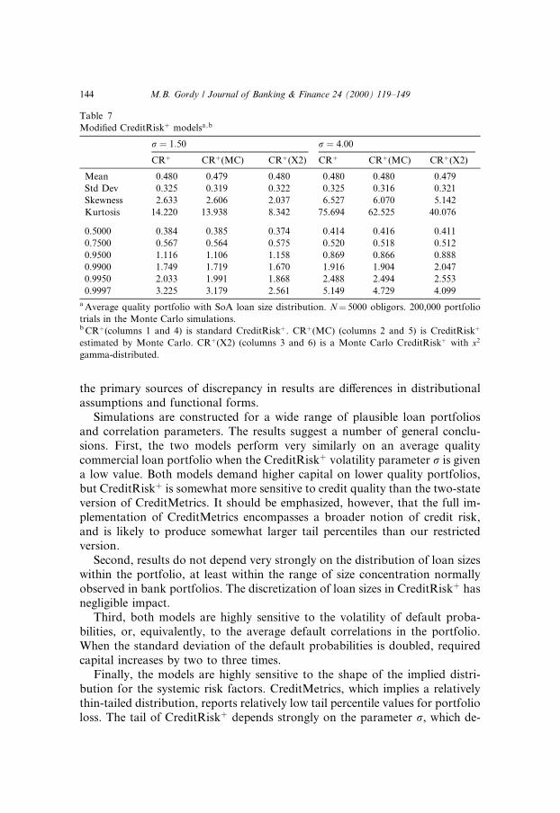
The results of both exercises on an Average quality portfolio are shown inTable 7. 28 The standard CreditRisk� results for r � 1:5 and r � 4:0 (columns1 and 4) are taken from Table 3. Results for the Monte Carlo version ofCreditRisk� are shown in columns 2 and 5. For the moderate value of r � 1:5,the 99.97th percentile value is reduced by under two percent. For the largervalue r � 4:0, however, the 99.97th percentile value is reduced by over eightpercent. The higher the value of r, the higher the probability of large condi-tional default probabilities. As the validity of the Poisson approximation thusbreaks down for high r, so does the accuracy of the analytic CreditRisk�

methodology.Results for the modi®ed CreditRisk� with x2 gamma-distributed are shown

in columns 3 and 6. For both values of r, the mean and standard deviation ofportfolio loss are roughly as before, but the tail percentiles are quite signi®-

28 Qualitatively similar results are found for portfolios based on the other credit quality

distributions.


cantly reduced. Indeed, the 99.97th percentile value for the modi®ed modelunder r � 1:5 is even less than the corresponding CreditMetrics value. Thisdemonstrates the critical importance of the shape of the distribution of thesystemic risk factor.

7. Discussion

This paper demonstrates that there is no unbridgeable di�erence in the viewsof portfolio credit risk embodied in CreditMetrics and CreditRisk�. If weconsider the restricted form of CreditMetrics used in the analysis, then eachmodel can be mapped into the mathematical framework of the other, so that

Fig. 2. Gamma and gamma-squared distributions.

Note: The two lines are cdfs of variables with mean one and variance one. If x is gamma distributed,

the solid line is its cdf. If x2 is gamma distributed, the dashed line is its cdf.


the primary sources of discrepancy in results are di�erences in distributionalassumptions and functional forms.

Simulations are constructed for a wide range of plausible loan portfoliosand correlation parameters. The results suggest a number of general conclu-sions. First, the two models perform very similarly on an average qualitycommercial loan portfolio when the CreditRisk� volatility parameter r is givena low value. Both models demand higher capital on lower quality portfolios,but CreditRisk� is somewhat more sensitive to credit quality than the two-stateversion of CreditMetrics. It should be emphasized, however, that the full im-plementation of CreditMetrics encompasses a broader notion of credit risk,and is likely to produce somewhat larger tail percentiles than our restrictedversion.

Second, results do not depend very strongly on the distribution of loan sizeswithin the portfolio, at least within the range of size concentration normallyobserved in bank portfolios. The discretization of loan sizes in CreditRisk� hasnegligible impact.

Third, both models are highly sensitive to the volatility of default proba-bilities, or, equivalently, to the average default correlations in the portfolio.When the standard deviation of the default probabilities is doubled, requiredcapital increases by two to three times.

Finally, the models are highly sensitive to the shape of the implied distri-bution for the systemic risk factors. CreditMetrics, which implies a relativelythin-tailed distribution, reports relatively low tail percentile values for portfolioloss. The tail of CreditRisk� depends strongly on the parameter r, which de-

Table 7

Modi®ed CreditRisk� modelsa;b

r � 1:50 r � 4:00

CR� CR�(MC) CR�(X2) CR� CR�(MC) CR�(X2)

Mean 0.480 0.479 0.480 0.480 0.480 0.479

Std Dev 0.325 0.319 0.322 0.325 0.316 0.321

Skewness 2.633 2.606 2.037 6.527 6.070 5.142

Kurtosis 14.220 13.938 8.342 75.694 62.525 40.076

0.5000 0.384 0.385 0.374 0.414 0.416 0.411

0.7500 0.567 0.564 0.575 0.520 0.518 0.512

0.9500 1.116 1.106 1.158 0.869 0.866 0.888

0.9900 1.749 1.719 1.670 1.916 1.904 2.047

0.9950 2.033 1.991 1.868 2.488 2.494 2.553

0.9997 3.225 3.179 2.561 5.149 4.729 4.099

a Average quality portfolio with SoA loan size distribution. N� 5000 obligors. 200,000 portfolio

trials in the Monte Carlo simulations.b CR�(columns 1 and 4) is standard CreditRisk�. CR�(MC) (columns 2 and 5) is CreditRisk�

estimated by Monte Carlo. CR�(X2) (columns 3 and 6) is a Monte Carlo CreditRisk� with x2

gamma-distributed.


termines the kurtosis (but not the mean or variance) of the distribution ofportfolio loss. Choosing less kurtotic alternatives to the gamma distributionused in CreditRisk� sharply reduces its tail percentile values for loss withouta�ecting the mean and variance.

This sensitivity ought to be of primary concern to practitioners. It is di�cultenough to measure expected default probabilities and their volatility. Capitaldecisions, however, depend on extreme tail percentile values of the loss dis-tribution, which in turn depend on higher moments of the distribution of thesystemic risk factors. These higher moments cannot be estimated with anyprecision given available data. Thus, the models are more likely to providereliable measures for comparing the relative levels of risk in two portfolios thanto establish authoritatively absolute levels of capital required for any givenportfolio.

Acknowledgements

I would like to thank David Jones for drawing my attention to this issue,and for his helpful comments. I am also grateful to Mark Carey for data andadvice useful in calibration of the models, and to Chris Finger, Tom Wilde andan anonymous referee for helpful comments. The views expressed herein aremy own and do not necessarily re¯ect those of the Board of Governors or itssta�.

Appendix A. Properties of the gamma distribution

The gamma distribution is a two parameter distribution commonly used intime-to-failure and other engineering applications. If x is distributed Gam-ma�a; b�, the probability density function of x is given by

f �xja; b� � xaÿ1 exp�ÿx=b�baC�a� ; �A:1�

where C�a� is the Gamma function. 29 The mean and variance of x are given byab and ab2, respectively. Therefore, if we impose E�x� � 1 and V �x� � r2, thenwe must have a � 1=r2 and b � r2.

29 Other parameterizations of this distribution are sometimes seen in the literature. This is the

parameterization used by CSFP (1997, Eq. 50).


Appendix B. Estimating the volatility of default probabilities

This appendix demonstrates a simple non-parametric method of estimatingthe volatility of default probabilities from historical performance data pub-lished by Standard & Poor's (Brand and Bahar, 1998, Table 12). Let pf�xt�denote the probability of default of a grade f obligor, conditional on the re-alized value xt of a systemic risk factor. We need to estimate the unconditionalvariance V �pf�x��. We assume that the xt are serially independent and thatobligor defaults are independent conditional on xt. Both CreditMetrics andCreditRisk� satisfy this framework, though the two models impose di�erentdistributional assumptions for x and functional forms for p�x�.

For each year in 1981±97 and for each rating grade, S&P reports the numberof corporate obligors in its ratings universe on January 1, and the number ofobligors who have defaulted by the end of the calendar year. Let d̂ft be thenumber of grade f defaults during year t, and let n̂ft denote the number ofgrade f obligors at the start of year t. Let p̂ft denote the observed defaultfrequency d̂ft=n̂ft. We assume that the size of the universe n̂ft is independent ofthe realization of xt.

The general rule for conditional variance is

V �y� � E�V �yjz�� V �E�yjz��: �B:1�Applied to the problem at hand, we have

V �p̂f� � E�V �p̂fjx; n̂f�� V �E�p̂fjx; n̂f��: �B:2�Obligor defaults are independent conditional on x, so d̂ft �Binomial(n̂ft; pf�xt�).The expectation of the conditional variance of p̂ft is therefore given by

E�V �p̂fjx; n̂f�� E�V �d̂fjx; n̂f�=n̂2f � � E�pf�x��1ÿ pf�x��=n̂f�

� E�1=n̂f��E�pf�x�� ÿ �V �pf�x�� E�pf�x��2�� E�1=n̂f��pf�1ÿ �pf� ÿ V �pf�x��;

�B:3�

where the second equality follows from the formula for the variance of a bi-nomial random variable, the third equality follows from the mutual indepen-dence of x and n̂f and the rule V �y� � E�y2� ÿ E�y�2; and the ®nal equality fromE�pf�x�� pf.

Since E�p̂fjx; n̂f� � pf�x�, the last term in Eq. (B.2) is simply V �pf�x��. Sub-stitute these simpli®ed expressions into Eq. (B.2) and rearrange to obtain

V �pf�x�� V �p̂f� ÿ E�1=n̂f��pf�1ÿ �pf�

1ÿ E�1=n̂f� : �B:4�

The values of �pf observed in the S&P data di�er slightly from the values usedfor calibration in Section 4.2. It is most convenient, therefore, to normalize theestimated default rate volatilities as ratios of the standard deviation of pf�x� to


its expected value,��V �pf�x��

p=�pf. In the ®rst two columns of Table 8, we

present for each rating grade the empirical values of �p and E�1=n̂� in the S&Pdata. The third column presents the observed variance of default rates, V̂ �p̂�,expressed in normalized form. The fourth column gives the implied normalizedvolatilities for the unobserved true conditional default probabilities.

For the highest grades, AAA and AA, no defaults occurred in the S&Psample, so it is impossible to estimate a volatility for these grades. Amongthe A obligors, only ®ve defaults were observed in the sample, so the defaultvolatility is undoubtedly measured with considerable imprecision. Therefore,calibration of the normalized volatilities for these grades requires somejudgment. Our chosen values for these ratios are given in the ®nal columnof Table 8. It is assumed that normalized volatilities are somewhat higherfor the top grades, but that the estimated value for grade A is implausiblyhigh. For the lower grades, the empirical estimates are made with greaterprecision (due to the larger number of defaults in sample), so these valuesare maintained.

Appendix C. Proof of Proposition 1

Let y1 and y2 be the CreditMetrics latent variables for two grade f obligors.Assume that there is only one systemic risk factor and that the two obligorshave the same weight wf on that risk factor. Thus,

yi � xwf ��1ÿ w2

f

q�i for i 2 f1; 2g: �C:1�

Conditional on x, default events for these obligors are independent, so

Pr�y1 < Cf & y2 < Cfjx� � Pr�y1 < Cfjx�Pr�y2 < Cfjx�

� U �Cf

�ÿ xwf�=

��1ÿ w2

f

q �2

� pf�x�2:�C:2�

Table 8

Empirical default frequency and volatility

�pf E�1=n̂f��V̂ �p̂f�

q=�pf

��V̂ �pf�x��

q=�pf

��Vfp

=�pf

AAA 0 0.0092 ± ± 1.4

AA 0 0.0030 ± ± 1.4

A 0.0005 0.0017 2.4857 1.5896 1.2

BBB 0.0018 0.0026 1.2477 0.3427 0.4

BB 0.0091 0.0038 1.2820 1.1108 1.1

B 0.0474 0.0041 0.6184 0.5492 0.55

CCC 0.1890 0.0360 0.5519 0.3945 0.4


Therefore,

Var�pf�x�� E�pf�x�2� ÿ E�pf�x��2

� E�Pr�y1 < Cf & y2 < Cfjx�� ÿ �p2f : �C:3�

Since y1 and y2 each have mean zero and variance one, and have correlation w2f ,

the unconditional expectation E�Pr�y1 < Cf & y2 < Cfjx�� is given byU�Cf;Cf;w2

f�. This gives

Var�pf�x�� U�Cf;Cf;w2f� ÿ �p2

f ; �C:4�as required.

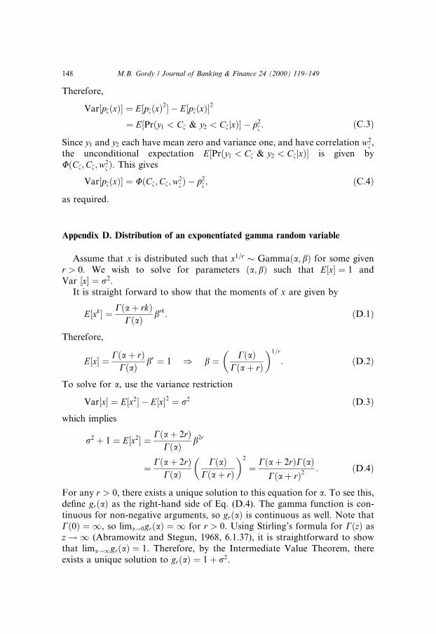
Appendix D. Distribution of an exponentiated gamma random variable

Assume that x is distributed such that x1=r � Gamma�a;b� for some givenr > 0. We wish to solve for parameters �a; b� such that E�x� � 1 andVar �x� � r2.

It is straight forward to show that the moments of x are given by

E�xk� � C�a� rk�C�a� brk: �D:1�

Therefore,

E�x� � C�a� r�C�a� br � 1 ) b � C�a�

C�a� r�� 1=r

: �D:2�

To solve for a, use the variance restriction

Var�x� � E�x2� ÿ E�x�2 � r2 �D:3�which implies

r2 � 1 � E�x2� � C�a� 2r�C�a� b2r

� C�a� 2r�C�a�

C�a�C�a� r�

� �2

� C�a� 2r�C�a�C�a� r�2 : �D:4�

For any r > 0, there exists a unique solution to this equation for a. To see this,de®ne gr�a� as the right-hand side of Eq. (D.4). The gamma function is con-tinuous for non-negative arguments, so gr�a� is continuous as well. Note thatC�0� � 1, so lima!0gr�a� � 1 for r > 0. Using Stirling's formula for C�z� asz!1 (Abramowitz and Stegun, 1968, 6.1.37), it is straightforward to showthat lima!1gr�a� � 1. Therefore, by the Intermediate Value Theorem, thereexists a unique solution to gr�a� � 1� r2.


References

Abramowitz, M., Stegun, I.A., 1968. Handbook of Mathematical Functions, Applied Mathematics

Series 55, National Bureau of Standards Gaithersburg, MD.

Belkin, B., Suchower, S., Forest, Jr., L.R., 1998. The e�ect of systematic credit risk on loan

portfolio value-at-risk and loan pricing, CreditMetrics Monitor, March, pp. 17±28.

Brand, L., Bahar, R., 1998. Ratings Performance 1997: Stability and Transition, Standard and

Poor's Special Report, August.

Carey, M., 1998. Credit risk in private debt portfolios. Journal of Finance 10 (10), 56±61.

Credit Suisse Financial Products, 1997. CreditRisk�: A CreditRisk Management Framework,

London.

Finger, C.C., 1998. Credit Derivatives in CreditMetrics, CreditMetrics Monitor, August, pp. 13±27.

Gordy, M.B., 1999. Calculation of Higher Moments in CreditRisk� with Applications, June.

Gupton, G.M., Finger, C.C., Bhatia, M., 1997. CreditMetrics-Technical Document. J.P. Morgan &

Co. Incorporated, New York, April.

Johnson, N.L., Kotz, S., 1969. Distributions in Statistics: Discrete Distributions, Houghton Mi�in,

Boston.

Koyluoglu, H.U., Hickman, A., 1998. Reconciliable di�erences. Risk 11 (10), 56±62.

Society of Actuaries, 1996. 1986±92 Credit Risk Loss Experience Study: Private Placement Bonds.

Schaumberg, IL.


a comparative anatomy of credit risk modelsrvicente/risco/gordy.pdf · with comparative analyses....

Documents