Advances in Water Resources 29 (2006) 899–911

www.elsevier.com/locate/advwatres

A comparative study of Monte Carlo simple genetic algorithmand noisy genetic algorithm for cost-effective sampling

network design under uncertainty

Jianfeng Wu a,b, Chunmiao Zheng b,*, Calvin C. Chien c, Li Zheng d

a Department of Earth Sciences, Nanjing University, Nanjing 210093, Chinab Department of Geological Sciences, 202 Bevill Research Building, University of Alabama, Tuscaloosa, AL 35487, United States

c Corporate Remediation, DuPont Company, Wilmington, DE 19805, United Statesd Agricultural Resources Research Center, IGDB, Chinese Academy of Sciences, Shijiazhuang 050021, China

Received 10 December 2004; received in revised form 12 August 2005; accepted 17 August 2005Available online 11 October 2005

Abstract

This study evaluates and compares two methodologies, Monte Carlo simple genetic algorithm (MCSGA) and noisy genetic algo-rithm (NGA), for cost-effective sampling network design in the presence of uncertainties in the hydraulic conductivity (K) field. Bothmethodologies couple a genetic algorithm (GA) with a numerical flow and transport simulator and a global plume estimator to iden-tify the optimal sampling network for contaminant plume monitoring. The MCSGA approach yields one optimal design each for alarge number of realizations generated to represent the uncertain K-field. A composite design is developed on the basis of thosepotential monitoring wells that are most frequently selected by the individual designs for different K-field realizations. The NGAapproach relies on a much smaller sample of K-field realizations and incorporates the average of objective functions associated withall K-field realizations directly into the GA operators, leading to a single optimal design. The efficacy of the MCSGA-based com-posite design and the NGA-based optimal design is assessed by applying them to 1000 realizations of the K-field and evaluating therelative errors of global mass and higher moments between the plume interpolated from a sampling network and that output by thetransport model without any interpolation. For the synthetic application examined in this study, the optimal sampling networkobtained using NGA achieves a potential cost savings of 45% while keeping the global mass and higher moment estimation errorscomparable to those errors obtained using MCSGA. The results of this study indicate that NGA can be used as a useful surrogate ofMCSGA for cost-effective sampling network design under uncertainty. Compared with MCSGA, NGA reduces the optimizationruntime by a factor of 6.5.� 2005 Elsevier Ltd. All rights reserved.

Keywords: Contaminant transport; Monitoring network design; Spatial moment analysis; Noisy genetic algorithm; Monte Carlo analysis; Uncer-tainty

1. Introduction

Since the early 1980s, the coupled simulation-optimi-zation model has increasingly become a valuable tool foranalyzing groundwater systems and managing ground-

0309-1708/$ - see front matter � 2005 Elsevier Ltd. All rights reserved.doi:10.1016/j.advwatres.2005.08.005

* Corresponding author. Tel.: +1 205 348 0579; fax: +1 205 3480818.

E-mail address: czheng@ua.edu (C. Zheng).

water resources [1,8,13,19,27,34,41,48–50,56]. A primarymotivation for the development of simulation-opti-mization models is the high costs associated withgroundwater quality management. A representative sim-ulation-optimization model is one that seeks to identifythe least-cost strategy to meet specified constraints. Inrecent years, the least-cost strategies are usually associ-ated with pump-and-treat or bioremediation design[2,5,30, 46,55].

900 J. Wu et al. / Advances in Water Resources 29 (2006) 899–911

Groundwater remediation often has time horizons of30 years or longer. Thus long-term monitoring of aremediation system�s performance is essential to ensurethat the remediation objectives are being achieved andthe risks to human health and environment are beingproperly managed [9]. Over-sampling is a commonproblem encountered in groundwater quality monitor-ing, where data collection and analysis of long-termmonitoring are expensive. Although the cost for an indi-vidual sampling data point may be relatively small, thescale of the required data collection effort over timecan make the cumulative costs very high. For a typicalgroundwater contamination site, several hundred sam-ples may be collected and analyzed each year that maycost hundreds of thousands of dollars. To prevent over-sampling, applications of simulation-optimization mod-els to long-term sampling network design can lead tosubstantial cost savings by eliminating or minimizingunnecessary samples [9]. This paper is intended to ad-dress simulation-optimization modeling for cost-effec-tive groundwater sampling network design in thepresence of uncertainties in the hydraulic conductivityfield.

Groundwater sampling network design has been stud-ied extensively in the past [3,4,6,10,11,21–23,25,29,31,32,36,39,42,43,51], and more recently the efforts haveoften focused on the least-cost strategies [43,39,51]. Theoptimization of sampling network design can be accom-plished using a variety of approaches as summarized in[35]. Selecting an appropriate method involves numerouscriteria, the most important of which include site-specificlong-term performance objectives and the amount andtype of available data. Reed et al. [39] presented an opti-mization methodology in which a genetic algorithm iscoupled with a flow and transport simulator and a globalmass estimator to search for optimal sampling strategies.Wu et al. [54] extended the methodology of Reed et al.[39] by introducing the first and second moments of aplume as additional constraints into the optimizationformulation. The methodology developed by Reedet al. [39] and extended by Wu et al. [54] does not addressuncertainties in the hydraulic conductivity field.

In reality, there always exists some amount of uncer-tainty in an aquifer simulation model. One of the mostimportant parameters, in terms of its contributions touncertainty, is hydraulic conductivity (K). In particular,the transport of contaminants in groundwater is domi-nated by the spatial variation of hydraulic conductivity.Sampling decisions will have to be made under consider-ation of uncertainties in the aquifer simulation model,and the reliability of model-based sampling decisions willbe a function of model uncertainties. A commonly usedapproach to dealing with the uncertainty in the K-fieldis the conditional Monte Carlo simulation based on acertain number of measured hydraulic conductivity data[12,26,31,32,47]. Although a number of studies have

incorporated uncertainties into the simulation-optimiza-tion model to design cost-effective sampling networksand determine the reliability of plume detection in clean-up systems of landfills and hazardous waste sites[11,31,32,47], the fundamental objectives of those studiesare substantially different from the goal of this study.

This study is intended to evaluate and compare twomethodologies for cost-effective sampling network de-sign under consideration of uncertainty. Both methodol-ogies couple a genetic algorithm with a numerical flowand transport simulator and a global plume estimatorto identify the optimal sampling network for contami-nant plume monitoring. Because a simple genetic algo-rithm cannot address uncertainty directly, othertechniques such as Monte Carlo simulation, stackingof K-field realizations, and chance constraints [5,15,32,37] must be used to incorporate uncertainty into asimple genetic algorithm. For the first methodology usedin this study, the Monte Carlo approach is adopted togenerate a large number of equally likely realizationsof the K field to account for the effect of uncertaintyon optimal network design. For the second methodol-ogy, a noisy genetic algorithm is adopted which wasdeveloped specifically to deal with uncertainty.

Unlike Monte Carlo simulation that requires a largenumber of samples to be drawn from the probability dis-tribution of the K-field to achieve sufficient accuracy, anoisy genetic algorithm can work well without extensivesampling from the realizations of the K-field [18,33,44,46]. Smalley et al. [46] successfully coupled a noisygenetic algorithm with a flow and transport model forpredicting concentrations in a risk-based in situ bio-remediation design system. Gopalakrishnan et al. [18]used a noisy genetic algorithm to identify the optimalgroundwater remediation design based on the assess-ment of risks to human health. To date, noisy geneticalgorithms have only been applied to remediation designassociated with groundwater quality management[18,46]. This study thus represents a first attempt toapply a noisy genetic algorithm to sampling networkdesign under uncertainty. To gain confidence in theapplicability and usefulness of noisy genetic algorithmsin solving sampling network design problems, this paperpresents a detailed comparison between a noisy geneticalgorithm and the Monte Carlo based approach.

This paper is organized in five sections. Following thisintroduction, we provide a brief overview of the simula-tion-optimization model used in this study for samplingnetwork design under deterministic conditions. We thendiscuss two methodologies, Monte Carlo simple geneticalgorithm and noisy genetic algorithm, for incorporatinguncertainties into the deterministic simulation-optimiza-tion model. Next we illustrate the two methodologies andcompare their performance in an application to a syn-thetic aquifer system. Finally we summarize the findingsand offer some concluding remarks.

J. Wu et al. / Advances in Water Resources 29 (2006) 899–911 901

2. Optimal monitoring network design

Wu et al. [54] presented a simulation-optimizationmethodology for cost-effective sampling network designunder deterministic conditions. Their methodology isan extension of Reed et al. [39] and is based on theminimization of total monitoring (capital and sam-pling) costs subject to two accuracy constraints. Forthe sake of completeness, the methodology of Wuet al. [54] is briefly recapitulated in this section. Formore detailed information, refer to Wu et al. [54] andReed et al. [39].

2.1. Numerical simulation and global plume estimation

The first step in the methodology of Wu et al. [54] isthe development of flow and transport models for thestudy site. This study utilizes the flow and transportmodels based on the three-dimensional finite-differenceflow code, MODFLOW [20,28], and its solute trans-port companion, MT3DMS [57]. The flow and trans-port codes are used to simulate the contaminantplume from the initial time to the end of the antici-pated monitoring period. The simulated plume repre-sents the future conditions to be monitored. If amodel node is selected as a potential monitoring welllocation, the simulated concentration value at thatlocation is considered known.

The second step is to use the known concentrations atall potential monitoring well locations to construct anapproximate new plume through interpolation. Theinterpolated plume is then compared, in terms of bothtotal mass as well as first and second moments, withthe simulated plume output from the transport modelwithout any interpolation. If enough nodes are selectedas potential monitoring well locations, the difference be-tween the simulated and interpolated plumes would beminimal. On the other hand, the more model nodesare selected as potential monitoring well locations, thehigher the capital and sampling costs would be. Thusthere exists a tradeoff between the accuracy of the inter-polated plume based on the sampled data and the cost-effectiveness of the sampling network.

An interpolation method, ordinary kriging (OK) [14],is applied to estimate contaminant concentrations at allunsampled nodes within the model domain. Then theOK-interpolated concentrations can be used for globalplume estimation to compare with that determined fromthe concentration distributions directly output from thetransport model without any interpolation. In thisstudy, the global plume estimation relates to three mo-ments, including the zeroth, first and second moments.The zeroth moment represents the global mass of theplume. The first and second moments specify the cen-troid of the plume and the spread of the plume aroundits centroid, respectively [16,36].

2.2. Objective function and constraints

The third step in the methodology of Wu et al. [54] isthe formulation of an optimization model. The objectiveof the optimization model is to minimize the total mon-itoring (installation/drilling and sampling) costs whilemaintaining the accuracy of global plume estimationbased on the sampled data. The monitoring networkdesign problem can thus be formulated as an optimalcontrol model with an objective function and a set ofconstraints [54]:

min J ¼ a1

Xn

i¼1

xili þ a2

Xn

i¼1

yidi ð1Þ

subject to emass 6 e1 ð2Þe1st 6 e2 ð3Þe2nd 6 e3 ð4Þ

where, in the objective function as given in (1), J is themanagement objective representing the total costs forsampling and well installation/drilling, n is the totalnumber of potential monitoring wells; a1 is the costfor each sampling, xi is a binary variable indicatingwhether sampling takes place at well i (yes if xi = 1;no if xi = 0), li is the number of sampling at different ele-vations for well i. If sampling takes place at well i, thewell i is selected to be sampled at multiple (i.e., li) eleva-tions. a2 is the fixed capital cost for installation/drillingper unit depth of well i, di denotes the depth of boreholeassociated with well i, and yi is a binary variable indicat-ing whether well i is drilled (yes if yi = 1; no if yi = 0).

The first constraint as expressed in Eq. (2) requiresthat the discrepancy, emass, be smaller than a prescribederror tolerance, e1, between the global mass of the com-plete solute plume as predicted by the solute transportmodel and that of the approximate solute plume inter-polated from the sampled data at the installed monitor-ing wells. The second and third constraints in Eqs. (3)and (4) require that both 1st and 2nd spatial momentsof the complete and approximate solute plumes as de-scribed above agree with each other within two sets ofpre-determined criteria, e2 and e3, respectively. e1st ande2nd are the weighted sum of errors for the respectivefirst and second moment estimations. Mathematically,the three constraints can be written as

emass ¼M0 �Mj

M0

����

���� ð5Þ

e1st ¼Xnd

k¼1

uk0;1 � uk

j;1

uk0;1

�����

�����xk1 ð6Þ

e2nd ¼X

k

uk0;2 � uk

j;2

uk0;2

�����

�����xk2 ð7Þ

where M0 is the contaminant mass in the area of interestas determined by the transport model, and Mj is the

902 J. Wu et al. / Advances in Water Resources 29 (2006) 899–911

approximate mass in the same area as determined by theglobal mass estimator based on the sampling design j,u0,i is the first or second moment of the simulated plumeas output from the transport model, uj,i is the corre-sponding moment estimated on the basis of the sam-pling design j, i denotes the order of moment (i.e., firstor second moment), nd denotes the dimension of theplume and is equal to 2 or 3, depending on the type ofthe flow and transport model, k is the direction alongwhich the moment is computed, and xk

i is the weight as-signed to the ith moment in the k-direction. For a three-dimensional problem, the second moment includes ninecomponent terms (reduced to six due to symmetry),whereas in a two-dimensional system, the secondmoment has only three component terms.

The constrained optimization problem as defined inEqs. (1)–(4) can be transformed into an easier-to-solveunconstrained one by adding the amount of any con-straint violation to the fitness function as a penalty. Thisis accomplished in this study by modifying Eqs. (1)–(4)as

min F ¼ J þ P 1 þ P 2 ð8Þwith

P 1 ¼ b1

emass � e1

e1

þ b2Nunestimate; e1 > 0 ð9Þ

P 2 ¼ b3½ðe1st � e2Þ þ ðe2nd � e3Þ� ð10Þ

where F is the penalized fitness value; P1 and P2 are thepenalty amounts of constraint violation with respect tothe global mass and higher moment estimation errors,respectively; Nunestimate is the number of points at whichthe concentration is not estimated as a result of no sam-pling data point within the specified search radius, andbi (i = 1, 2, 3) is penalty coefficients. The specified searchradius is defined a maximal distance of search for knowndata (concentrations) around an unestimated point.

2.3. Solution by genetic algorithms

The final step in the methodology of Wu et al. [54] isto find the optimal sampling plan from among manyalternatives using the genetic algorithm (GA) [17,38,45]. In recent years, GA has been shown to be a valuabletool for solving complex optimization problems inbroad fields, including groundwater management andmonitoring network design [2,7,11, 24,30,40,51–53,55].For any sampling network design problem, a numberof potential sampling locations may be specified. TheGA considers each sampling alternative design to be astring (chromosome) consisting of zero-one variables,where the value of 1 in the ith digit (bit) represents sam-pling from the ith potential location, and 0 no sampling.The total number of nonzero digits in the string denotesthe number of sampling locations used in the currentdesign. In this study, a simple GA procedure was used

that consisted of 60 generations with a population of800 individuals (chromosomes) in each generation. Fora more thorough discussion of using GA in the contextof sampling network design, refer to [39,54].

3. Methodologies for dealing with uncertainty

A simple genetic algorithm (SGA) cannot explicitlyaddress the uncertainty in the aquifer simulation modelarising from insufficient hydraulic conductivity data.Methodologies for dealing with uncertainty in optimiza-tion modeling are reviewed by Freeze and Gorelick [15].This study evaluates and contrasts two methodologies inthe context of monitoring network design. First, SGA iscombined with Monte Carlo simulation in what is re-ferred to as Monte Carlo simple genetic algorithm(MCSGA). Second, SGA is applied in a noisy environ-ment in what is referred to as noisy genetic algorithm(NGA) [18,33,46].

3.1. Monte Carlo simple genetic algorithm

A commonly used stochastic approach for accommo-dating the uncertainty arising from insufficient hydraulicconductivity data needed for a groundwater model isMonte Carlo simulation in which multiple realizationsof the hydraulic conductivity field are generated[12,31,32,47]. Each realization is equally likely in the sta-tistical sense, and can be further conditioned to the sameset of known hydraulic conductivity data. The flow andtransport model must be run for each K realization,leading to a range of calculated head and concentrationdistributions. It is noteworthy that several assumptionsare associated with the Monte Carlo methodologyapplied in this study, including, (1) the hydraulic con-ductivity field follows a log-normal distribution, (2)the hydraulic conductivity field is ergodic and has sta-tionary second moment, and (3) the spatial correlationis defined as an isotropic, exponential covariance func-tion [46].

For each realization of the hydraulic conductivityfield, the sampling network design problem becomes adeterministic one and can be solved independently usingthe simple genetic algorithm as described in Section 2. Inthis manner, the optimal or near-optimal designs corre-sponding to all realizations of the K-field can be ob-tained and evaluated. These designs are interim, eachof which only satisfies the constraints associated with aparticular K realization. Subsequently, a composite de-sign can be developed on the basis of those potentialmonitoring wells that are most frequently selected bythe individual interim designs for different K realiza-tions. Since several hundred or more K realizationsmay be required for adequate representation of theuncertainty in the K-field, the MCSGA approach is time

Individual 1Individual 2 . . . Individual npopsiz

Flow & Transportfor K Realization #1

Gen #1

Individual 1Individual 2 . . .

Gen #2

. . .

Optimal Design #1

. . . . . .

Individual 1Individual 2 . . . Gen #1

Individual 1Individual 2 . . .

Gen #2

. . .

Gen #1

Gen #2

. . .

K1 K2 Kn1. . .

Avg. OBF 1Avg. OBF 2Avg. OBF 3

K1 K2 K'n2. . .

Avg. OBF 1Avg. OBF 2Avg. OBF 3

' '

Optimal Design

Flow &Transport Simulations for each Selected K Realization

. . .

. . .. . .

Optimal Design #2

Flow & Transportfor K Realization #2

Flow &Transport Simulations for each Selected K Realization

(a) (b)

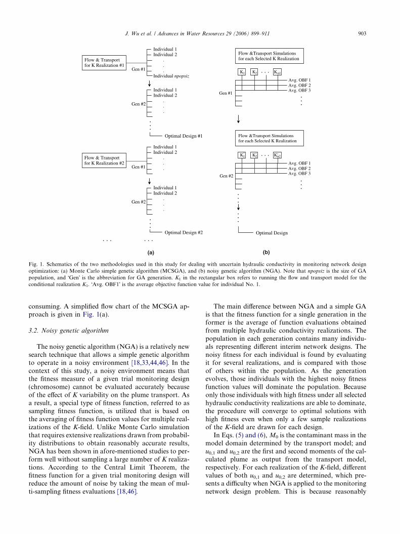
Fig. 1. Schematics of the two methodologies used in this study for dealing with uncertain hydraulic conductivity in monitoring network designoptimization: (a) Monte Carlo simple genetic algorithm (MCSGA), and (b) noisy genetic algorithm (NGA). Note that npopsiz is the size of GApopulation, and �Gen� is the abbreviation for GA generation. K1 in the rectangular box refers to running the flow and transport model for theconditional realization K1. �Avg. OBF1� is the average objective function value for individual No. 1.

J. Wu et al. / Advances in Water Resources 29 (2006) 899–911 903

consuming. A simplified flow chart of the MCSGA ap-proach is given in Fig. 1(a).

3.2. Noisy genetic algorithm

The noisy genetic algorithm (NGA) is a relatively newsearch technique that allows a simple genetic algorithmto operate in a noisy environment [18,33,44,46]. In thecontext of this study, a noisy environment means thatthe fitness measure of a given trial monitoring design(chromosome) cannot be evaluated accurately becauseof the effect of K variability on the plume transport. Asa result, a special type of fitness function, referred to assampling fitness function, is utilized that is based onthe averaging of fitness function values for multiple real-izations of the K-field. Unlike Monte Carlo simulationthat requires extensive realizations drawn from probabil-ity distributions to obtain reasonably accurate results,NGA has been shown in afore-mentioned studies to per-form well without sampling a large number of K realiza-tions. According to the Central Limit Theorem, thefitness function for a given trial monitoring design willreduce the amount of noise by taking the mean of mul-ti-sampling fitness evaluations [18,46].

The main difference between NGA and a simple GAis that the fitness function for a single generation in theformer is the average of function evaluations obtainedfrom multiple hydraulic conductivity realizations. Thepopulation in each generation contains many individu-als representing different interim network designs. Thenoisy fitness for each individual is found by evaluatingit for several realizations, and is compared with thoseof others within the population. As the generationevolves, those individuals with the highest noisy fitnessfunction values will dominate the population. Becauseonly those individuals with high fitness under all selectedhydraulic conductivity realizations are able to dominate,the procedure will converge to optimal solutions withhigh fitness even when only a few sample realizationsof the K-field are drawn for each design.

In Eqs. (5) and (6), M0 is the contaminant mass in themodel domain determined by the transport model; andu0,1 and u0,2 are the first and second moments of the cal-culated plume as output from the transport model,respectively. For each realization of the K-field, differentvalues of both u0,1 and u0,2 are determined, which pre-sents a difficulty when NGA is applied to the monitoringnetwork design problem. This is because reasonably

904 J. Wu et al. / Advances in Water Resources 29 (2006) 899–911

accurate and stationary values of u0,1 and u0,2 are neededas common references for comparison of potential de-signs associated with different hydraulic conductivityrealizations. To overcome this difficulty, it is assumedthat u0,1 and u0,2, along with M0, can be determinedfrom the plume resulting from the kriged K-field basedon the measured K data at a set of known locations.This assumption is consistent with the practice in whichthe K distribution for a field-scale model is often inter-polated from the measured data by the kriging methodand used as the basis for monitoring network design.Fig. 1(b) illustrates the framework used in this studyfor cost-effective monitoring network design based onNGA.

In this study, K-field sampling is done through a ran-dom number generator with each random number corre-sponding to a particular realization among all therealizations generated a priori. A potential monitoringdesign is evaluated for each K realization by runningthe flow and transport model and determining the objec-tive function and constraint violations. Then the overallfitness of any given potential design is set to the averageof its fitness values associated with every selected K real-ization [18,46].

Note that the methodologies presented in this studyidentify the optimal sampling design for only one mon-itoring period. For the monitoring network design prob-lems with multiple monitoring periods, the value of yi in

No Flow Bou

No Flow Bou

Con

stan

t Hea

d B

ound

ary

1 2 3 4 5 6

9 10 11 12 13 14

18 19 20 21 22 23

27 28 29 30 31 32

36 37 38 39 40 41

46 47 48 49 50 51

55 56 57 58 59 60

65 66 67 68

h=89.0 m

h=89.5 m

400

m

600 m

64

Fig. 2. Configuration of the monitoring network design problem. The solid tropen circles denote the optimal monitoring wells selected by NGA. The colorof the monitoring period output by the transport model for the hydraulic cond

Eq. (1) is 1 when the ith monitoring location is selectedfor a particular monitoring period; and the value of yi

remains 0 for all other periods since the capital costshould be counted only once. Also, the fixed capital costis generally more expensive than the sampling cost atany monitoring location, and thus the network designfor one monitoring period affects those of other periods.Accordingly, for the multi-period monitoring networkdesign problems, the optimal network designs for differ-ent monitoring periods are not independent.

4. Application to a synthetic aquifer system

4.1. Description of the application

The hypothetical application used in this study in-volves a two-dimensional confined aquifer measuring600 m long in the x-direction and 400 m wide in they-direction. Fig. 2 shows the plan view of the syntheticaquifer and the block-centered finite difference mesh.The aquifer is surrounded by a constant-head boundaryalong the left side, a specified-flux boundary with a con-stant inflow rate along the right side, and no-flowboundaries along the upper and lower sides. Thehydraulic conductivity distribution in the aquifer isisotropic and represented by a log-normally distributed,spatially-correlated random field. Other properties in-

ndary

ndary

Con

stan

t Rec

harg

e F

lux

Bou

ndar

y 7 8

15 16 17

24 25 26

33 34 35

42 43 44 45

52 53 54

61 62 63

69 70

Source

2

5

10

20

30

40

50

60

70

ppb

71

iangles indicate the pre-defined potential monitoring well locations. The-filled contour map represents the concentration distribution at the enductivity field kriged using 62 known K values (shown as open squares).

Table 1Primary input data used in this studya

Parameter Value

Porosity 0.175Aquifer thickness 10.0 mLongitudinal dispersivity 8.5 mRatio of horizontal transverse to

longitudinal dispersivity0.1

Constant flux along the specified-flow boundary 9.45 m/dayMean of lnK 2.2 m/dayVariance of lnK 0.30Correlation scale of hydraulic conductivity 100.0 mGrid spacing along column 20.0 mGrid spacing along row 20.0 m

a Modified from Wagner [51].

1 11 21 31 41 51 61 71

Potential Location Number

0.0

0.2

0.4

0.6

0.8

1.0

Sam

pled

Pro

babi

lity

Fig. 3. Relative frequency of each pre-defined potential monitoringwell selected by the individual optimal designs obtained using MCSGAfor 1000 conditional realizations of the K-field. The columns of shadedcolor denote the optimal monitoring locations selected by NGA.

J. Wu et al. / Advances in Water Resources 29 (2006) 899–911 905

cluding porosity, thickness, and dispersivities are con-stant throughout the aquifer system. Key input dataused in the flow and transport model and K field gener-ation are listed in Table 1. The flow and transport modelfor the application is based on a version of MODFLOW[28] and MT3DMS [57] codes.

Sequential Gaussian simulation (SGSIM) [14] wasused to generate 1000 equally likely realizations of theK-field, based on the lnK statistical parameters (mean,variance, and correlation length) listed in Table 1. Thehydraulic conductivity was assumed to be known at 62measurement locations (see scattered square symbolsin Fig. 2) within the aquifer, with the mean and varianceof lnK equal to 2.2 and 0.3, respectively. The K valuesranged from a minimum of 2.6 m/day to a maximumof 30.0 m/day. All 1000 K realizations were conditionedto the 62 K data.

An instant spill was assumed to occur at the sourcearea (c0 = 1000.0 ppb) that resulted in a contaminantplume migrating toward the left boundary (see Fig. 2).The plume shown in Fig. 2 was obtained by the trans-port model for the K-field kriged from the 62 knownK data. The total simulation time was three years, themonitoring period considered in this application. A totalof 71 potential monitoring locations were initially se-lected as shown in Fig. 2. The total mass and the firstand second moments for the interpolated plume basedon the 71 monitoring locations were in reasonably closeagreement with those calculated directly from the outputof the transport model.

In this study, the operational cost for sampling (a1li)and the fixed cost for installation/drilling (a2di) wereboth taken to be $2000 for each monitoring well. Wuet al. [54] pointed out that the penalty costs set approx-imately 5–20 times the expected real monitoring costswould result in an optimal or near-optimal sampling de-sign that is both cost-effective and sufficiently accuratein terms of mass and higher moment estimations. More-over, the number of sampling data is always much smal-ler than the total number of model nodes in a numericalsimulation model, thus it is rather difficult to reduce the

second moment estimation errors, making it necessaryto set the error tolerance for the plume moment con-straints as small as possible [54]. Considering thisapproximate rule of setting penalty coefficients and theexpected number of monitoring wells in this example,the coefficients for the fitness objective function givenin Eqs. (8)–(10) were set as follows: b1 = 5.0 · 104,b2 = 50, b3 = 3.0 · 105, e1 = 0.05, and e2 = e3 = 0. Allweights assigned to the higher moments along differentdirections are set equal, i.e., xk

i ¼ 1 in Eqs. (6) and (7).

4.2. Solution based on Monte Carlo simple genetic

algorithm

For each conditional realization of the K-field, thesimple genetic algorithm was applied to identify a moni-toring network that is optimal specific to the associated K

realization. As a result, a total of 1000 individual optimaldesigns were obtained corresponding to 1000 K realiza-tions. Fig. 3 shows how frequently each of the 71 poten-tial monitoring wells is selected by any of the 1000individual optimal designs. From a comparison of Figs.3 and 2, it is evident that the monitoring wells either closeto the plume centroid or near the edges have a greaterprobability of being chosen by one or more optimal de-signs. This is because overall the interpolated plumebased on those monitoring wells is more likely to matchthe plume directly output from the transport model.

Fig. 4 is a scatter diagram showing the relative errorsof the interpolated plume based on each monitoring net-work for a corresponding K realization. The relative er-rors are expressed in terms of the differences in globalmass and higher moments between the interpolatedplume and the reference plume output by the trans-port model without any interpolation. The average rela-tive errors of global mass and first moments for allmonitoring designs are quite small, at 4.17% and

Fig. 4. Comparison of relative estimation errors of global mass and higher moments for 1000 realizations of the K-field under different networkdesign methodologies. The errors are computed as the relative differences between the plume interpolated from the optimal monitoring wells and thatgiven by the transport model without any interpolation for 1000 conditional realizations of the K-field.

Table 2Statistics of relative estimation errors for optimal monitoring network designs obtained using different methodologies

Itema MCSGA Composite MCSGA NGA

mass l1 l2 mass l1 l2 mass l1 l2

Minimum 0.0000 0.0007 0.2348 0.0000 0.0006 0.1247 0.0000 0.0006 0.2321Maximum 0.3180 0.0860 1.8290 0.1287 0.0671 1.1909 0.1566 0.0844 1.4825Mean 0.0417 0.0293 0.6965 0.0312 0.0189 0.3151 .0547 0.0309 0.5397Standard deviation 0.0323 0.0150 0.2901 0.0230 0.0103 0.1239 0.0277 0.0156 0.1913

a The items of mass, l1 and l2 represent the relative estimation errors for the mass, first and second moments of the plume, respectively.

906 J. Wu et al. / Advances in Water Resources 29 (2006) 899–911

2.93%, respectively, but that of second moments is sub-stantially larger at 69.65% (Table 2). This can be attrib-

uted to the significant variation of plume shape causedby the variability in the K-field.

25 30 35 40 45 50Number of Monitoring Wells in the Optimal Design

0.00

0.02

0.04

0.06

0.08

0.10

Rel

ativ

e F

requ

ency

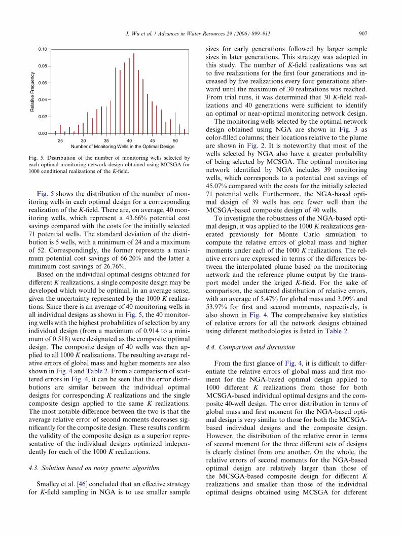
Fig. 5. Distribution of the number of monitoring wells selected byeach optimal monitoring network design obtained using MCSGA for1000 conditional realizations of the K-field.

J. Wu et al. / Advances in Water Resources 29 (2006) 899–911 907

Fig. 5 shows the distribution of the number of mon-itoring wells in each optimal design for a correspondingrealization of the K-field. There are, on average, 40 mon-itoring wells, which represent a 43.66% potential costsavings compared with the costs for the initially selected71 potential wells. The standard deviation of the distri-bution is 5 wells, with a minimum of 24 and a maximumof 52. Correspondingly, the former represents a maxi-mum potential cost savings of 66.20% and the latter aminimum cost savings of 26.76%.

Based on the individual optimal designs obtained fordifferent K realizations, a single composite design may bedeveloped which would be optimal, in an average sense,given the uncertainty represented by the 1000 K realiza-tions. Since there is an average of 40 monitoring wells inall individual designs as shown in Fig. 5, the 40 monitor-ing wells with the highest probabilities of selection by anyindividual design (from a maximum of 0.914 to a mini-mum of 0.518) were designated as the composite optimaldesign. The composite design of 40 wells was then ap-plied to all 1000 K realizations. The resulting average rel-ative errors of global mass and higher moments are alsoshown in Fig. 4 and Table 2. From a comparison of scat-tered errors in Fig. 4, it can be seen that the error distri-butions are similar between the individual optimaldesigns for corresponding K realizations and the singlecomposite design applied to the same K realizations.The most notable difference between the two is that theaverage relative error of second moments decreases sig-nificantly for the composite design. These results confirmthe validity of the composite design as a superior repre-sentative of the individual designs optimized indepen-dently for each of the 1000 K realizations.

4.3. Solution based on noisy genetic algorithm

Smalley et al. [46] concluded that an effective strategyfor K-field sampling in NGA is to use smaller sample

sizes for early generations followed by larger samplesizes in later generations. This strategy was adopted inthis study. The number of K-field realizations was setto five realizations for the first four generations and in-creased by five realizations every four generations after-ward until the maximum of 30 realizations was reached.From trial runs, it was determined that 30 K-field real-izations and 40 generations were sufficient to identifyan optimal or near-optimal monitoring network design.

The monitoring wells selected by the optimal networkdesign obtained using NGA are shown in Fig. 3 ascolor-filled columns; their locations relative to the plumeare shown in Fig. 2. It is noteworthy that most of thewells selected by NGA also have a greater probabilityof being selected by MCSGA. The optimal monitoringnetwork identified by NGA includes 39 monitoringwells, which corresponds to a potential cost savings of45.07% compared with the costs for the initially selected71 potential wells. Furthermore, the NGA-based opti-mal design of 39 wells has one fewer well than theMCSGA-based composite design of 40 wells.

To investigate the robustness of the NGA-based opti-mal design, it was applied to the 1000 K realizations gen-erated previously for Monte Carlo simulation tocompute the relative errors of global mass and highermoments under each of the 1000 K realizations. The rel-ative errors are expressed in terms of the differences be-tween the interpolated plume based on the monitoringnetwork and the reference plume output by the trans-port model under the kriged K-field. For the sake ofcomparison, the scattered distribution of relative errors,with an average of 5.47% for global mass and 3.09% and53.97% for first and second moments, respectively, isalso shown in Fig. 4. The comprehensive key statisticsof relative errors for all the network designs obtainedusing different methodologies is listed in Table 2.

4.4. Comparison and discussion

From the first glance of Fig. 4, it is difficult to differ-entiate the relative errors of global mass and first mo-ment for the NGA-based optimal design applied to1000 different K realizations from those for bothMCSGA-based individual optimal designs and the com-posite 40-well design. The error distribution in terms ofglobal mass and first moment for the NGA-based opti-mal design is very similar to those for both the MCSGA-based individual designs and the composite design.However, the distribution of the relative error in termsof second moment for the three different sets of designsis clearly distinct from one another. On the whole, therelative errors of second moments for the NGA-basedoptimal design are relatively larger than those ofthe MCSGA-based composite design for different Krealizations and smaller than those of the individualoptimal designs obtained using MCSGA for different

Fig. 6. Comparison of relative estimation errors of global mass andhigher moments in terms of PDF and CDF for optimal networkdesigns obtained using different methodologies.

908 J. Wu et al. / Advances in Water Resources 29 (2006) 899–911

K realizations. As shown in Table 2, the average relativeerrors of global mass, first and second moments are4.17%, 2.93% and 69.65%, respectively, for the individ-ual optimal designs obtained using MCSGA for the1000 K realizations. The average relative errors of globalmass and first moments are sufficiently small. However,due to significant variations in K realizations to whichthe second moments are very sensitive, the average rela-tive error of second moments is substantially larger. TheMCSGA-based 40-well composite design has averagerelative errors of 3.12%, 1.89%, and 31.51% for globalmass, first and second moments, respectively, whichare lower than those computed for the individual opti-mal designs. Thus the composite design can be consid-ered an optimal representative of the 1000 individualoptimal designs. The single optimal design obtainedusing NGA, when applied to the same 1000 K realiza-tions, resulted in average relative errors of 5.47%,3.09%, and 53.97% for global mass, first and second mo-ments, respectively. The average relative errors of globalmass and first moment for the NGA optimal design areclose to those for both MCSGA-based individual opti-mal designs and the composite 40-well design. However,the average relative error of second moments for theNGA optimal design is smaller than that of theMCSGA-based individual optimal designs, but largerthan that of the MCSGA-based composite 40-welldesign.

To further validate the result from the NGA, Fig. 6shows a visual comparison of the histograms (discreteprobability density function or discrete PDF) and cumu-lative distribution function (CDF) for relative errors ofglobal mass, first and second moment estimates, respec-tively. Fig. 6(a) indicates that the range of distributionfor the global mass errors based on the NGA design isclose to that based on the MCSGA individual designs,even though the former has an greater mean than thelatter (5.47% vs. 4.17%). Overall, the differences amongMCSGA-based and NGA-based designs are insignifi-cant. Fig. 6(b) shows the distribution of the first momenterrors. The difference between the NGA- and MCSGA-based designs is almost negligible. While the error distri-bution for the MCSGA-based composite 40-well designis defined more narrowly and sharply, the overall distri-butions for the first moment errors are similar and suf-ficiently small for all three cases. Fig. 6(c) shows thedifferences among the three cases for the second momenterrors. The MCSGA-based composite 40-well design ismost satisfactory, with smaller errors than both theNGA-based design and MCSGA-based individual de-signs. However, the shape of CDF for the NGA-baseddesign is similar to that for the MCSGA-based compos-ite 40-well design, which is sharper than that for theMCSGA-based individual designs. Also, compared withthe MCSGA-based individual designs, the error distri-bution for the NGA-based design has a smaller mean

and narrower range. Overall, the optimal design identi-fied by NGA appears to be an acceptable surrogate forthe MCSGA-based designs.

Computationally, NGA is much more efficient thanMCSGA. In this study, completion of an optimizationrun based on MCSGA requires a total run time ofapproximately 170 hours on a desktop PC equippedwith a 2.20 GHz Pentium-4 CPU. In contrast, the com-pletion of a run based on NGA requires only 26 hourson the same PC. For real-world applications, MCSGAmay become computationally prohibitive. The resultsof this study show that NGA can find the near-optimal

J. Wu et al. / Advances in Water Resources 29 (2006) 899–911 909

sampling design, and the distribution of global mass andhigher moment estimation errors based on the NGA de-sign have statistical traits similar to those based onMCSGA. Thus with its computational efficiency androbustness, NGA may represent a promising alternativeto MCSGA for real-world applications to design themost cost-effective groundwater monitoring networksunder uncertainty.

5. Conclusions

We have evaluated and compared two methodolo-gies, Monte Carlo simple genetic algorithm (MCSGA)and noisy genetic algorithm (NGA), for incorporatingthe uncertainty in the K-field into cost-effective monitor-ing network design problems. Both methodologies cou-ple a genetic algorithm with a numerical flow andtransport simulator and a global plume estimator toidentify the optimal sampling network for contaminantplume monitoring. However, they differ in the handlingof the K-field uncertainty. MCSGA utilizes a sufficientlylarge number of realizations of the K-field for adequateuncertainty representation, and identifies an optimalmonitoring network design for each realization. A limi-tation of this approach is that the multiple designs can-not be applied directly to a real field application. Acomposite design, however, can be developed on thebasis of those potential monitoring wells that are mostfrequently selected by individual designs under differentK-field realizations. NGA, on the other hand, relies on amuch smaller sample of K-field realizations, and incor-porates the average of objective functions associatedwith all K-field realizations into the GA operators, toidentify a single optimal design.

For the application example examined in this paper,the optimal network design obtained using NGAachieves a potential cost savings of 45.07% while main-taining acceptable accuracy in global mass and highermoment estimations. The estimation error distributionsobtained by applying the NGA optimal design to multi-ple realizations of the K-field closely agree with thoseobtained by applying the simple genetic algorithm toall individual realizations of the K-field (MCSGA). Thisindicates that NGA can be used as an effective surro-gate of MCSGA for cost-effective monitoring networkdesign under uncertainty. Compared with MCSGA,NGA is much more efficient computationally, by a fac-tor of 6.5 for this study, and results in a uniquesolution.

While this study has demonstrated the advantages ofusing NGA to accommodate uncertainty of hydraulicconductivity in monitoring network design, further re-search is needed to investigate how the methodologycan be improved to further reduce the estimation errorsof plume moments and how the K-field statistics and

sampling strategies as well as GA solution parame-ters affect the computational accuracy and efficiency.Moreover, further study is needed to demonstrate theapplicability and flexibility of the NGA methodologyat large-scale field sites.

Acknowledgments

This study was supported in part by DuPont Com-pany and the National Natural Science Foundation ofChina (Nos. 40472130 and 40335045). Additionalsupport was provided by the Innovation Project (GrantNo. KZCX3-SW-428) of Chinese Academy of Sci-ences. We are indebted to Gaisheng Liu who providedthe initial code for computing the spatial momentsof a contaminant plume. The authors are also grate-ful to the four anonymous reviewers whose construc-tive comments helped to improve the manuscriptsignificantly.

References

[1] Ahlfeld DP, Mulvey JM, Pinder GF. Contaminated groundwaterremediation design using simulation, optimization, and sensitivitytheory. 2. Analysis of a field site. Water Resour Res 1988;24(5):443–52.

[2] Aly AH, Peralta RC. Optimal design of aquifer cleanup systemsunder uncertainty using a neural network and a genetic algorithm.Water Resour Res 1999;35(8):2523–32.

[3] Andricevic R. Coupled withdrawal and sampling designs forgroundwater supply models. Water Resour Res 1993;29(1):5–16.

[4] Andricevic R. Evaluation of sampling in the subsurface. WaterResour Res 1996;32(4):863–74.

[5] Bear J, Sun Y. Optimization of pump-treat-inject (PTI) design forthe remediation of a contaminated aquifer: multi-stage designwith chance constraints. J Contam Hydrol 1998;29:225–44.

[6] Bogaert P, Russo D. Optimal spatial sampling design for theestimation of the variogram based on a squares approach. WaterResour Res 1999;35(4):1275–89.

[7] Cai X, McKinney DC, Lasdon LS. Solving nonlinear watermanagement models using a combined genetic algorithm andlinear programming approach. Adv Water Resour 2001;24:667–76.

[8] Cai X, Rosegrant MW, Ringler C. Physical and economicefficiency of water use in the river basin: implications forefficient water management. Water Resour Res 2003;39(1):1013.doi:10.1029/2001WR000748.

[9] Chien CC, Medina Jr MA, Pinder GF, Reible DR, Sleep BE,Zheng C, editors. Contaminated ground water and sediment,modeling for management and remediation. Boca Raton, Flor-ida: Lewis Publishers; 2004. p. 274.

[10] Christakos G, Killam BR. Sampling design for classifyingcontamination level using annealing search algorithm. WaterResour Res 1993;29(12):4063–76.

[11] Cieniawski SE, Eheart JW, Ranjithan S. Using genetic algorithmto solve a multiobjective groundwater monitoring problem. WaterResour Res 1995;31(2):399–409.

[12] Copty NK, Findikakis AN. Quantitative estimates of the uncer-tainty in the evaluation of ground water remediation schemes.Ground Water 2000;38(1):29–37.

910 J. Wu et al. / Advances in Water Resources 29 (2006) 899–911

[13] Culver TB, Shoemaker CA. Dynamic optimal control forgroundwater remediation with flexible management periods.Water Resour Res 1992;28(3):629–41.

[14] Deutsch CV, Journel AG. GSLIB: geostatistical software libraryand user�s guide. 2nd ed. New York: Oxford University Press;1998.

[15] Freeze RA, Gorelick SM. Convergence of stochastic optimizationand decision analysis in the engineering design of aquiferremediation. Ground Water 1999;37(6):934–54.

[16] Freyberg DL. A natural gradient experiment on solute transport ina sand aquifer: 2. Spatial moments and the advection and dispersionof nonreactive tracers. Water Resour Res 1986;22(13): 2031–46.

[17] Goldberg DE. Genetic algorithm in search, optimization andmachine learning. Reading, MA: Addison Wesley; 1989.

[18] Gopalakrishnan G, Minsker BS, Goldberg D. Optimal samplingin a noisy genetic algorithm for risk-based remediation design. In:Phelps D, Sehlke G, editors. Bridging the gap: meeting the world�swater and environmental resources challenges. Proc world waterand environmental resources congress. Washington DC: ASCE;2001.

[19] Gorelick SM. A review of distributed parameter groundwatermanagement modeling method. Water Resour Res 1983;19(2):305–19.

[20] Harbaugh AW, Banta ER, Hill MC, McDonald MG. MOD-FLOW-2000, the US Geological Survey modular ground-watermodel–user guide to modularization concepts and the ground-water flow process. USGS Open-File Report 00-92, 2000. p. 121.

[21] Hudak PF, Loaiciga HA. A location modeling approach forgroundwater monitoring network augmentation. Water ResourRes 1992;28(3):643–9.

[22] Hudak PF, Loaiciga HA. An optimization method for monitoringnetwork design in multilayered groundwater flow system. WaterResour Res 1993;29(8):2835–45.

[23] James BR, Gorelick SM. When enough is enough: the worth ofmonitoring data in aquifer remediation design. Water Resour Res1994;30(12):3499–513.

[24] Lee Y-M, Ellis JH. Comparison of algorithms for nonlinearinteger optimization: application to monitoring network design. JEnviron Eng 1996;122(6):524–31.

[25] Loaiciga H. An optimization approach for groundwater qualitymonitoring network design. Water Resour Res 1989;25(8):1771–80.

[26] Maxwell RD, Kastenberg WE, Rubin Y. A methodology tointegrate site characterization information into groundwater-driven health risk assessment. Water Resour Res 1999;35(9):2841–55.

[27] Mayer AS, Kelley CT, Miller CT. Optimal design for problemsinvolving flow and transport phenomena in saturated subsurfacesystems. Adv Water Resour 2002;25:1233–56.

[28] McDonald MG, Harbaugh AW. A modular three-dimensionalfinite-difference ground water flow model. USGS Techniques ofWater Resources Investigations, Book 6, 1988.

[29] McKinney DC, Loucks DP. Network design for predictinggroundwater contamination. Water Resour Res 1992;28(1):133–47.

[30] McKinney DC, Lin MD. Genetic algorithm solution of ground-water management models. Water Resour Res 1994;30(6):1897–906.

[31] Meyer PD, Valocchi AJ, Eheart JW. Monitoring network designto provide initial detection of groundwater contamination. WaterResour Res 1994;30(9):2647–59.

[32] Meyer PD, Eheart JW, Ranjithan S, Valocchi AJ. Design ofgroundwater monitoring networks for landfills. In: KundzewiczZW, editor. Proc international workshop on new uncertaintyconcepts in hydrology and water resources. Cambridge, 1995.p. 190–6.

[33] Miller BL. Noise, sampling, and efficient genetic algorithms. PhDdissertation, University of Ill, Urbana-Champaign, 1997.

[34] Minsker BS, Shoemaker CA. Dynamic optimal control of in situbioremediation of ground water. J Water Resour Plann Manage1998;124(3):149–61.

[35] Minsker BS, editor. Long-term groundwater monitoring: thestate of the art. Reston, VA: ASCE/EWRI; 2003, ISBN 0-7844-0678-2.

[36] Montas HJ, Mohtar RH, Hassan AE, AlKhal FA. Heuristicspace-time design of monitoring wells for contaminant plumecharacterization in stochastic flow fields. J Contam Hydrol2000;43:271–301.

[37] Morgan DR, Eheart JW, Valocchi AJ. Aquifer remediation designunder uncertainty using a new chance constraints programmingtechnique. Water Resour Res 1993;29(3):551–61.

[38] Pham DT, Karaboga D. Intelligent optimization techniques:genetic algorithms, tabu search, simulated annealing and neuralnetworks. New York: Springer-Verlag; 2000.

[39] Reed PB, Minsker B, Valocchi AJ. Cost-effective long-termgroundwater monitoring design using a genetic algorithm andglobal mass interpolation. Water Resour Res 2000;36(12):3731–41.

[40] Ritzel BJ, Eheart JW, Ranjithan S. Using genetic algorithms tosolve a multiple-objective groundwater pollution containmentproblem. Water Resour Res 1994;30(5):1589–603.

[41] Rizzo DM, Dougherty DE. Design optimization for multiplemanagement period groundwater remediation. Water Resour Res1996;32(8):2549–61.

[42] Rouhani S, Hall TJ. Geostatistical schemes for groundwatersampling. J Hydrol 1988;103:85–120.

[43] Rouhani S. Variance reduction analysis. Water Resour Res 1985;21(6):837–46.

[44] Sano Y, Kita H. Optimization of noisy fitness functions by meansof genetic algorithms using history of search. In: Schoenauer M,Deb K, Rudolph G, Yao X, Lutton E, Merelo JJ, et al., editors.Proc 6th international conference on parallel problem solving fornature. Springer-Verlag; 2000. p. 571–81.

[45] Sen M, Stoffa PL. Global optimization methods in geophysicalinversion. Elesevier Science Publishers; 1995.

[46] Smalley JB, Minsker B, Goldberg DE. Risk-based in situbioremediation design using a noisy genetic algorithm. WaterResour Res 2000;36(10):3043–52.

[47] Storck P, Eheart JW, Valocchi AJ. A method for the optimallocation of monitoring wells for detection of groundwatercontamination in three-dimensional aquifers. Water Resour Res1997;33(9):2081–8.

[48] Tiedeman C, Gorelick SM. Analysis of uncertainty in optimalgroundwater contaminant capture design. Water Resour Res1993;29(7):2139–54.

[49] Wagner BJ, Gorelick SM. Reliable aquifer remediation in thepresence of spatially variable hydraulic conductivity: from data todesign. Water Resour Res 1989;25(10):2211–25.

[50] Wagner BJ. Recent advances in simulation-optimization ground-water management modeling. Review of geophysics. US NationalReport to International Union of Geodesy and Geophysics 1991–1994, Suppl, 1995. p. 1021–8.

[51] Wagner BJ. Sampling design methods for groundwater modelingunder uncertainty. Water Resour Res 1995;31(10):2581–91.

[52] Wang CG, Jamieson DG. An objective approach to regionalwastewater treatment planning. Water Resour Res 2002;38(3).doi:10.1029/2000WR000062.

[53] Wang M, Zheng C. Optimal remediation policy selection undergeneral conditions. Ground Water 1997;35(5):757–64.

[54] Wu J-F, Zheng C, Chien CC. Cost effective sampling networkdesign for contaminant plume monitoring under general hydro-geological conditions. J Contam Hydrol 2005;77:41–65.

J. Wu et al. / Advances in Water Resources 29 (2006) 899–911 911

[55] Zheng C, Wang PP. A field demonstration of the simulation-optimization approach for remediation system design. GroundWater 2002;40(3):258–65.

[56] Zheng C, Wang PP. An integrated global and local optimizationapproach for remediation system design. Water Resour Res 1999;35(1):137–48.

[57] Zheng C, Wang PP. MT3DMS: a modular three-dimensionalmultispecies transport model for simulation of advection, disper-sion and chemical reactions of contaminants in ground watersystems: Documentation and user�s guide. Contract ReportSERDP-99-1, US Army Engineer Research and DevelopmentCenter, Vicksburg, Mississippi, 1999.