a comparative verification of forecasts from · pdf filea comparative verification of...

AFRL-RV-PS- AFRL-RV-PS- TP-2012-0006 TP-2012-0006 A COMPARATIVE VERIFICATION OF FORECASTS FROM TWO OPERATIONAL SOLAR WIND MODELS (POSTPRINT) Donald C. Norquist and Warner C. Meeks 8 February 2012 Technical Paper

APPROVED FOR PUBLIC RELEASE; DISTRIBUTION IS UNLIMITED.

AIR FORCE RESEARCH LABORATORY Space Vehicles Directorate 3550 Aberdeen Ave SE AIR FORCE MATERIEL COMMAND KIRTLAND AIR FORCE BASE, NM 87117-5776

REPORT DOCUMENTATION PAGE Form Approved

OMB No. 0704-0188 Public reporting burden for this collection of information is estimated to average 1 hour per response, including the time for reviewing instructions, searching existing data sources, gathering and maintaining the data needed, and completing and reviewing this collection of information. Send comments regarding this burden estimate or any other aspect of this collection of information, including suggestions for reducing this burden to Department of Defense, Washington Headquarters Services, Directorate for Information Operations and Reports (0704-0188), 1215 Jefferson Davis Highway, Suite 1204, Arlington, VA 22202-4302. Respondents should be aware that notwithstanding any other provision of law, no person shall be subject to any penalty for failing to comply with a collection of information if it does not display a currently valid OMB control number. PLEASE DO NOT RETURN YOUR FORM TO THE ABOVE ADDRESS. 1. REPORT DATE (DD-MM-YYYY) 08-02-2012

2. REPORT TYPE Technical Paper

3. DATES COVERED (From - To) 1 Oct 2007 – 16 Dec 2010

4. TITLE AND SUBTITLE A Comparative Verification of Forecasts from Two Operational Solar Wind Models (Postprint)

5a. CONTRACT NUMBER

(Postprint)

5b. GRANT NUMBER

5c. PROGRAM ELEMENT NUMBER 62601F

6. AUTHOR(S) Donald C. Norquist and Warner C. Meeks

5d. PROJECT NUMBER 1010

5e. TASK NUMBER PPM00004579

5f. WORK UNIT NUMBER EF004380 7. PERFORMING ORGANIZATION NAME(S) AND ADDRESS(ES)

AND ADDRESS(ES)

8. PERFORMING ORGANIZATION REPORT NUMBER

Air Force Research Laboratory Space Vehicles Directorate 3550 Aberdeen Ave SE Kirtland AFB, NM 87117-5776

AFRL-RV-PS-TP-2012-0006

9. SPONSORING / MONITORING AGENCY NAME(S) AND ADDRESS(ES) 10. SPONSOR/MONITOR’S ACRONYM(S) AFRL/RVBXS 11. SPONSOR/MONITOR’S REPORT NUMBER(S) 12. DISTRIBUTION / AVAILABILITY STATEMENT Approved for public release; distribution is unlimited. (66ABW-2010-0714 dtd 4 Jun 2010) 13. SUPPLEMENTARY NOTES Space Weather, 8, S12005, doi:10.1029/2010SW000598, 2010. Government purpose rights.

14. ABSTRACT In this study we evaluate and compare forecasts from two models that predict SW and IMF conditions: the Hakamada-Akasofu-Fry (HAF) version 2, operational at the Air Force Weather Agency, and Wang-Sheeley-Arge (WSA) version 1.6, executed routinely at the Space Weather Prediction Center. SW speed (Vsw) and IMF polarity (Bpol) forecasts at L1 were compared with Wind and Advanced Composition Explorer satellite observations. Verification statistics were computed by study year and forecast day. Results revealed that both model’s mean Vsw are slower than observed. Neither model had skill above a random guess in predicting Vsw increase arrival time at L1.

15. SUBJECT TERMS Solar wind models, Interplanetary magnetic field, Hakamada-Akasofu-Fry (HAF), Wang-Sheeley-Arge (WSA)

16. SECURITY CLASSIFICATION OF:

17. LIMITATION OF ABSTRACT

18. NUMBER OF PAGES

19a. NAME OF RESPONSIBLE PERSON Donald Norquist

a. REPORT Unclassified

b. ABSTRACT Unclassified

c. THIS PAGE Unclassified

Unlimited

19b. TELEPHONE NUMBER (include area

code) Standard Form 298 (Rev. 8-98)

Prescribed by ANSI Std. 239.18

20

A comparative verification of forecasts from twooperational solar wind models

Donald C. Norquist1 and Warner C. Meeks1

Received 8 June 2010; revised 4 September 2010; accepted 15 September 2010; published 16 December 2010.

[1] The solar wind (SW) and interplanetary magnetic field (IMF) have a significant influence on thenear‐Earth space environment. In this study we evaluate and compare forecasts from two models thatpredict SW and IMF conditions: the Hakamada‐Akasofu‐Fry (HAF) version 2, operational at the AirForce Weather Agency, and Wang‐Sheeley‐Arge (WSA) version 1.6, executed routinely at the SpaceWeather Prediction Center. SW speed (Vsw) and IMF polarity (Bpol) forecasts at L1 were comparedwith Wind and Advanced Composition Explorer satellite observations. Verification statistics werecomputed by study year and forecast day. Results revealed that both models’ mean Vsw are slowerthan observed. The HAF slow bias increases with forecast duration. WSA had lower Vsw forecast‐observation difference (F‐O) absolute means and standard deviations than HAF. HAF and WSA Vsw

forecast standard deviations were less than observed. Vsw F‐O mean square skill rarely exceeds that ofrecurrence forecasts. Bpol is correctly predicted 65%–85% of the time in both models. Recurrencebeats the models in Bpol skill in nearly every year forecast day category. Verification by “event” (flareevents ≤5 days before forecast start) and “nonevent” (no flares) forecasts showed that most HAFVsw bias growth, F‐O standard deviation decrease, and forecast standard deviation decrease were due tothe event forecasts. Analysis of single time step Vsw increases of ≥20% in the nonevent forecastsindicated that both models predicted too many occurrences and missed many observed incidences.Neither model had skill above a random guess in predicting Vsw increase arrival time at L1.

Citation: Norquist, D. C., and W. C. Meeks (2010), A comparative verification of forecasts from two operationalsolar wind models, Space Weather, 8, S12005, doi:10.1029/2010SW000598.

1. Introduction[2] The accuracy of solar wind and interplanetary

magnetic field (IMF) predictions near Earth is an impor-tant factor in anticipating their effects on key spaceweather forecast parameters such as geomagnetic indexand magnetic flux. It is useful to document the char-acteristics of a solar wind and IMF prediction model’sperformance for several reasons. Developers of the modelcan identify strengths and weaknesses to effectively focustheir improvement efforts. Authors of other models aremade aware of the formulation/deficiency relationshipscommon to such models. Quantifying the accuracy of themodel forecasting capabilities can help numerical mode-lers who may use the forecast output as input to drivetheir numerical simulations. In the operational commu-nity, forecasters gain by knowing how much confidence toplace on predicted parameters. Cost/benefit information isprovided to administrators who decide to sustain or

replace existing models. Continuous monitoring of fore-cast performance can help identify changes in the mea-surements of instruments used to supply the referencedata.[3] Previous solar wind model forecast verification

studies were designed to assess the performance of long‐term simulations. Owens et al. [2008] used magnetic fieldmaps constructed for entire Carrington rotations (that is,the approximately 27 day full solar rotation) to producesolar wind speed forecasts with three models. Solar windmodels evaluated were the Wang‐Sheeley‐Arge (WSA)coronal/heliospheric model [Arge and Pizzo, 2000; Argeet al., 2004], the WSA coronal model coupled with theENLIL heliospheric model [Odstrcil, 2003], and the Mag-netohydrodynamics Around a Sphere (MAS) coronalmodel [Linker et al., 1999; Mikić et al., 1999] coupled withthe ENLIL heliospheric model (together called CORHEL).Forecasts from the period 1995–2002 were compared withhourly observations to compute forecast, observation, andforecast‐observation difference (“error”) statistics. Theobservations were from the Wind and Advanced Com-position Explorer (ACE) satellites positioned at the L1Lagrangian point approximately 1.5M km upstream of

1Battlespace Environment Division, Space Vehicles Directorate,Air Force Research Laboratory, Hanscom Air Force Base,Massachusetts, USA.

SPACE WEATHER, VOL. 8, S12005, doi:10.1029/2010SW000598, 2010

S12005Copyright 2010 by the American Geophysical Union 1 of 16

Approved for public release; distribution is unlimited.

Earth. Using point‐by‐point statistical analysis techniquesto assess the forecast performance of the models, theyfound that the kinematic WSA model produced solar windspeed forecasts that showed greater skill than the coupledWSA/ENLIL and CORHEL models. Lee et al. [2009] com-pared WSA/ENLIL and CORHEL solar wind forecastsusing Carrington rotation magnetic field maps in 2003–2005 with ACE spacecraft measurements at L1. Theyshowed many results from single Carrington rotations andcomposite histograms emphasizing the general large‐scalesolar wind structures from the model predictions andobservations. Overall they found satisfactory agreement ofthe model solar wind and IMF predictions with theobserved conditions. MacNeice [2009] ran version 1.6 ofthe WSA coronal/heliospheric model for Carringtonrotations spanning 32 years (1977–2008), assessing the skillscore and event probabilities of solar wind speed and IMFpolarity predictions for each rotation. Carrington mag-netic field maps were used from three solar observatorieswith each having separate parameter values specified inthe radial velocity formula on the inner boundary. Theinner boundary radius had two settings, 5 and 21.5 solarradii. Observations at L1 were used as a reference forcomputing forecast skill. Computing skill score withrespect to persistence (actual measured value 1, 2, 4, and8 days before the forecast valid date) as a reference, hefound that WSA forecasts at L1 were competitive withpersistence after 2 days of forecast time and surpass it inskill at the 4 and 8 day forecast times. The model per-formance was not significantly sensitive to source of thesolar magnetic field data, the inner boundary radius of theWSA model, or whether the period of the solar cycleevaluated was quiet or active. WSA was better at pre-dicting polarity reversal events than it was in forecastinghigh‐speed events: percentage of correct forecasts (hitrate) were 61% and 40%, respectively, and percentage ofincorrectly predicted event occurrence (false positive rate)of 11% and 39%, respectively.[4] In this article we describe a study of the forecast

performance of two operational solar wind models: theHakamada‐Akasofu‐Fry (HAF) version 2 kinematic modelcurrently used at the Air Force Weather Agency, and theWSA version 1.6 coronal/heliospheric model that was theversion executed daily at the Space Weather PredictionCenter of the National Oceanic and AtmosphericAdministration as of mid‐2009. We felt it was important todocument the performance of these models as a baselineagainst which any replacement candidate model shouldbe assessed. From the standpoint of an operational fore-caster, there is interest in the day‐to‐day changes in thepredicted state from a simulation initialized from the mostrecently observed conditions. Thus in this study we usethe daily updated photospheric magnetic field maps as theinitial conditions to drive the forecasts of the two opera-tional models. As in the previously cited studies, wecompared the forecasts of solar wind and IMF at L1 withWind and ACE observations. We evaluated the forecastseparately by forecast day in each of 6 years to investigate

the dependence of model performance on forecast dura-tion, often referred to as lead time. Forecast performancefor particular years can thus be assessed as a way ofdetermining the sensitivity of the models to solar activitylevel.[5] Following this introduction, the article discusses the

models and data used in this forecast verification study insection 2. Section 3 is a description of the forecast verifi-cation method. In section 4 we present the verificationresults from all forecasts. Separate statistics are thenpresented for the forecasts with and without solar dis-turbances in the 5 days prior to forecast initiation. Thissection concludes with the results of a brief study on theability of the two models to predict single time stepincreases in solar wind speed. Section 5 closes the articlewith a summary and conclusions.

2. Data and Forecast Models[6] The available daily magnetic field maps from the

Mount Wilson Observatory (MWO) in California, referredto as the MWO Coarse Synoptic Magnetogram maps,were obtained for the odd numbered years of Solar Cycle23: 1997, 1999, 2001, 2003, 2005, and 2007. These years wereselected as the periods for model evaluation in this studyas a compromise between keeping the number of forecastsexecuted/evaluated to a manageable size yet coveringrepresentative portions of a complete solar cycle. Eachavailable data file represents a date during which photo-spheric magnetic field measurements were usually takenaround local noon, weather permitting. For California, thiscorresponds to approximately 2000 UTC for much of theyear. To account for a reasonable amount of processingtime, the source surface map generated from each day’smagnetogram map was used to initialize a HAF or WSAforecast beginning at 0000 UTC on the following day.[7] The daily magnetogram map files consist of mag-

netic field values on a grid of 4° longitude by roughly4.6° latitude (equally spaced in sine latitude). These gridsextend longitudinally around the solar sphere betweenroughly ±76° latitude. The observations taken on thespecified date of the file had been assimilated into theprevious day’s grid values as a daily update in the visibleportion of the Sun. Missing data near the poles werefilled in by assigning the polewardmost available value ateach longitude to the missing grid points. In some casesall values along a longitude were missing. If such a datagap was ≤20° in longitude width, the magnetic field valuesof each latitude on the bounding longitudes were linearlyinterpolated to fill in the missing values of that latitude inthe data gap. If the gap was greater, the magnetogrammap file was not considered available for initialization ofthe models. The following numbers of daily magnetic fieldfiles (out of 365 possible) were available for model runs inthe 6 years study, respectively: 272, 266, 248, 240, 231, and284 for a total of 1,541 HAF and WSA forecasts.[8] TheHAF version 2 [Fry et al., 2001] is a kinematic solar

wind model, essentially an empirical parameterization

NORQUIST AND MEEKS: SOLAR WIND FORECAST MODELS S12005S12005

2 of 16


of plasma parcel motion, and does not contain full phys-ical representations as does a magnetohydrodynamic(MHD) model. It runs much more quickly than an MHDmodel (about 6 s on a high‐end workstation) and canaccept rather steep spatial and temporal gradients on theinner boundary. The radial, kinematic expansion of theejected coronal plasma and the frozen‐in magnetic fielddefines the solar wind structure. HAF tracks the solarwind fluid parcels and the interplanetary magnetic fieldlines, capturing the large‐scale solar wind as it flowsoutward from the Sun. However, the model does notprovide information on the detailed energetics of the solarwind flow, nor does it resolve the small‐scale waves andturbulence. HAF predicts solar wind speed, density, andmagnetic field strength and orientation. In the simulationof the solar wind flow from the Sun to the Earth, radialspeed is computed from the positions of the fluid parcelsat successive time steps. Magnetic flux conservation isassumed for the computation of the magnetic field vector,and density is computed by assuming a conservation ofmass flux. Dynamic pressure, and for events the shockarrival time (SAT) at L1, are derived from the predictedvariables.[9] HAF simulates the stream‐stream interaction

regions through parameterized compression‐rarefactionalgorithms. Projected plasma parcels encounter theseinteractions, arriving at the L1 point with a resultingspeed that is registered as the Vsw prediction. HAF alsosimulates the plasma motion associated with nonuniformbackground flow resulting from solar disturbances. Flaresand associated coronal mass ejections (CME) drive shockwaves in the plasma that represent the leading edge ofthe propagating disturbance. Such a disturbance is con-sidered an “event” for which radio, optical and X‐rayobservations are used to specify its characteristics in HAF.These flare properties are used as input to HAF in a list ofany solar flare events that occurred in the 5 days prior tothe initial time of the model execution. As explained byFry et al. [2001], CME‐generating disturbance events usedin HAF are restricted to flares since it is difficult to specifythe source information for other CME initiation me-chanisms. The master list of all solar flare events used toconstruct each flare property input file for the HAFforecast executions is the same as that used in the three‐phase “Fearless Forecast” project [Fry et al., 2003;McKenna‐Lawlor et al., 2006; Smith et al., 2009]. If no flareevents occurred in the 5 days prior to the forecast initialtime, the input file was blank, and the execution wasconsidered a “nonevent” forecast. In HAF, a discontinuityin dynamic pressure (proportional to the product ofdensity and the square of speed) represents a proxy forthe shock.[10] HAF outputs radial speed, density, magnetic field

magnitude and three components of the magnetic fieldvector in the geocentric solar magnetospheric (GSM)coordinate system at each hour of forecast time. For anexample of a time series plot of HAF forecast output, seeFry et al. [2001]. Because of the comparative nature of this

study, only solar wind speed (Vsw) and IMF polarity (Bpol,±1 derived from the component of the magnetic fieldvector along the Sun‐Earth line) were considered sinceWSA only predicted these two quantities. A verification ofall HAF output variables over the same study years wasdone by Norquist [2010]. Fry et al. [2003], McKenna‐Lawloret al. [2006], and Smith et al. [2009] have conducted acomprehensive evaluation of the prediction of SAT byHAF.[11] In preprocessing for the HAF model executions,

the available daily MWO magnetic field maps wereinterpolated to a regular 5° × 5° latitude‐longitude grid.Next, the potential field source surface (PFSS) model[Altschuler and Newkirk, 1969] was executed on each mapto extend the magnetic field from the photosphere out to2.5 RS in the corona also on the 5° × 5° grid. Then thevelocity on the source surface at 2.5 RS was computed byan empirical algorithm that assumes that the radialvelocity on the source surface depends only on thedivergence of the magnetic flux between the photosphereand the source surface. The empirical parameters in theformula are adjusted to best reproduce the observedspeed at L1, and were constant for all forecasts in thisstudy. After their ingest into HAF, the source surfacemagnetic field and radial velocity were interpolated toabout half‐degree spacing in order for HAF to produceforecasts on 1 h time steps. Each daily source surfacemap serves as the inner boundary condition for the 5 dayHAF model execution initialized at 0000 UTC on thefollowing day.[12] Arge et al. [2004] give a detailed description of the

WSA solar wind model. The design and forecast initiali-zation procedures of the WSA have been described byMacNeice [2009]. Our remarks are thus limited to modelaspects relevant to its execution in this study. It has innercorona, outer corona and inner heliosphere componentsthat act in succession to propel the solar plasma fromregions of open field lines in the photosphere to L1. Theinner corona module of WSA uses essentially the samePFSS model as used in HAF preprocessing to extend thephotosphere radial magnetic field maps out to a prelim-inary source surface at 2.5 RS on a 2.5° latitude‐longitudegrid. The coronal extension component of the WSAmodel is the Schatten current sheet model [Schatten, 1971]that we used to compute the radial magnetic field on asource surface at 5 RS. Next, WSA invokes the empiricalscheme [Arge et al., 2004] based on magnetic fieldexpansion factors and angular distance from the nearestcoronal hole boundary to compute Vsw on this outersource surface. The one‐dimensional inner heliospherecomponent transported the plasma parcels radially out-ward with this flow speed. The parcels were acceleratedor slowed by interaction with faster parcels from behindor slower parcels lying ahead as they propagated out toL1 and beyond. The magnetic field (magnitude andpolarity, which is negative sunward and positive anti-sunward) determined on the outer source surface issimilarly subject to modification due to interaction with


3 of 16


adjacent parcels in its transit to L1. Because of the 2.5°outer source surface grid, the WSA time step is approx-imately 4.55 h.[13] Both forecast models were initialized with the

same available MWO photospheric magnetic field mapsto ensure direct comparability. The models were exe-cuted to predict Vsw and Bpol at their respective time stepintervals over the same calendar date periods. Hourlyaveraged solar wind speed and magnetic field observa-tions from the Wind (1997) and ACE (1999, 2001, 2003,2005, and 2007) satellites at L1 served as a reference forthe forecast verifications. The hourly observation timesnearest the forecast valid times of the WSA time steps ofeach forecast day were chosen as a basis for verification.Typically, there were 26 time steps in the 5 day forecastperiods whose average temporal separation from thenearest hour was approximately 15 min. Then the samehourly HAF time steps were extracted from their forecastfiles to represent the HAF predictions to be verified.There were periods of missing observations but they onlyamounted to about a 2% data loss for Vsw and less than1% for Bpol among the hourly values used in the ver-ifications. Occasionally (in 0.02% of the hourly outputs)HAF produced an excessive single hour value of Vsw thatis readily apparent in the time series plots from eachforecast execution. To preserve the integrity of the veri-fication statistics, any Vsw prediction exceeding 150% ofthe maximum observed Vsw was not verified. Given thenumber of available forecasts in the 6 study years aslisted above, the number of forecast time steps for veri-fication in each forecast day ranged from a low of about1,200 in 2005 to a high of just over 1,500 in 2007.[14] Both HAF forecasts and ACE and Wind observa-

tions provide magnetic field vector at L1 in the threecomponents of the GSM coordinate system. To renderthem directly comparable with WSA‐predicted Bpol at L1,the x component (directed sunward from Earth) sign wasnoted. Positive values (sunward directed) were assignedas Bpol = −1 and negative values (antisunward) as Bpol = +1in concert with WSA IMF polarity convention.[15] Though the observations serve as a reference

against which the forecast parameters can be evaluated,they must be qualified in their use as such a reference.There are several considerations that indicate that theyare not an exact representation of the environmentaltruth that the model was attempting to predict. First, theforecasts represent a grid volume while observations arepoint measurements. This suggests a certain degree ofspatial smoothing associated with the forecasts. Second,the forecasts represent a discrete time, while Wind andACE hourly average values are the result of averagingmany individual measurements over the hour followingthe forecast valid time (ACE Science Center, ACE dataprocessing and archiving, 2010; available at http://www.srl.caltech.edu/ACE/ASC/docs/processing.html; see alsoMIT Space Plasma Group, Wind‐SWE data page, 2010;available at http://web.mit.edu/space/www/wind/wind_data.html). Third, the sensors are subject to occasional

solar wind and IMF disturbances, elevating parameterlevels to the point where the WIND and ACE sensors canbe overwhelmed and fail to produce accurate readings(ACE Science Center, ACE data processing and archiv-ing, 2010; available at http://www.srl.caltech.edu/ACE/ASC/docs/processing.html). Fourth, the instrument sen-sitivity threshold dictates that very small parameter va-lues, particularly for density, can lead to inaccurateWIND and ACE sensor measurements. For these rea-sons, this study refers to discrepancies between predictedand observed parameter values as differences rather thanerrors. Over a large sample of comparisons, as is carriedout in this study, the errors in the observations tend toaverage out provided there is no systematic drift in thesensor. Therefore, the forecast‐observation difference canbe thought of as a possible model deficiency. But it mustbe kept in mind that some portion of that difference isdue to the disparities in the source of the forecast andobserved value making up the difference as mentionedabove.

3. Forecast Verification Method[16] Forecast verification by individual year allows for a

look at the effect of solar activity variation on model per-formance. In each year’s evaluation, the forecast valueswere verified in daylong lead time interval groups: 1–24 h,25–48 h, 49–72 h, 73–96 h, and 97–120 h corresponding todays 1–5. Such a partitioning lets us examine forecast skillas a function of the forecast lead time. This is of interest tothe operational forecaster who must assign a level ofreliability to the guidance provided by each day’s multi-day forecast.[17] As mentioned in section 2, forecast‐observation

difference represents the best measure of the forecastdeficiency considering the representativeness issues. At asingle model time step, this difference quantifies howmuch the forecast misses the mark in terms of providinga preview of future conditions at L1. The differencebetween mean value of the forecasts and the mean valueof the observations is a systematic error called bias. If themodel predicts a variable with a small mean error but alarge variation in the forecast‐observation difference, themodel performs poorly in matching the temporal varia-tion of the observed state. So both the systematic andrandom components of the forecast‐observation differ-ence tell a story about the nature of the model’s forecastperformance. In this study we sought to examine bothcomponents to most fully evaluate each model’s predic-tive ability.[18] For solar wind speed we were able to compute a

full range of forecast‐observation difference (F‐O) sta-tistics. Representing the F‐O of a parameter x at eachhour i by

Xi ¼ xFi � xOi ;


4 of 16


where F and O designate the forecast and observedvalues, respectively, the following F‐O statistics werecomputed:mean,

X ¼ 1N

XNi¼1

Xi;

mean square,

X2 ¼ 1N

XNi¼1

X2i ;

standard deviation,

�X ¼ffiffiffiffiffiffiffiffiffiffiffiffiffiffiffiffiffiffiffiffiffiffiffiffiffiffiffiffiffiffiffiffi1N

XNi¼1

Xi � X� �2

vuut ;

absolute mean,

X�� ¼ 1

N

XNi¼1

Xij j;

skill score,

SS ¼ 1� X2=P2; Pi ¼ xOi¼0 � xOi ;

in which Pi is the persistence F‐O, subtracting theobserved value nearest each forecast time step from theobserved value at the initial time (0 h) of the 5 dayforecast. This initial observed value is held constant(“persisted”) over the entire forecast period and servesas the forecast value at all time steps in this simplistictype of forecast. In all statistical quantities, the sum-mation is over N forecast time steps in each daylonglead time interval group over all available forecasts in astudy year. In the skill score, the persistence forecastserves as a baseline. A skill score value of 1 (variabledifference mean square = 0) means that the forecastmatched the observations perfectly. With a skill score of0 the evaluated model predicts the observations nobetter than persistence, while negative values denotepoorer agreement with observations than persistence.[19] An alternative baseline forecast against which a

model prediction can be compared in skill score isrecurrence. Because the Sun rotates with a period ofapproximately 27 days, operational forecasters often takeadvantage of the long‐lasting nature of some major solarfeatures (e.g., coronal holes) in making space weatherpredictions. The state of forecast parameters of interest27 days prior to the forecast valid date are commonly usedas a “first guess” for the formulation of a forecast. Rec-ognizing the fact that the solar period is not exactly 27 daysand that, while general features may remain their spatialdetail can change significantly during Sun’s revolution, weused the daily averaged observations from 27 days prioras the recurrence forecast. Norquist [2010] showed thatthe daily average recurrence consistently demonstratessuperior skill over hourly recurrence (27 days prior to the

hour nearest the time step valid time). Skill scores basedon day average recurrence were also computed in theHAF and WSA Vsw forecast verification.[20] Correlation of the forecast values with the observed

values is a quantitative measure of how well the temporalvariations match. It can be computed for both the timestep value pairs and the day average value pairs. In eithercase, the correlation is computed using the respectivemeansand standard deviations of the forecast and observed values,then using them to compute the correlation:mean,

xF ¼ 1N

XNi¼1

xFi ; xO ¼ 1N

XNi¼1

xOi ;

standard deviation,

�xF ¼ffiffiffiffiffiffiffiffiffiffiffiffiffiffiffiffiffiffiffiffiffiffiffiffiffiffiffiffiffiffiffiffiffi1N

XNi¼1

xFi � xFð Þ2vuut ; �xO ¼

ffiffiffiffiffiffiffiffiffiffiffiffiffiffiffiffiffiffiffiffiffiffiffiffiffiffiffiffiffiffiffiffiffiffiffi1N

XNi¼1

xOi � xOð Þ2vuut ;

correlation,

rxFxO ¼

1N

XNi¼1

xFi � xFð Þ xOi � xOð Þ

�xF�xO;

where the xF, xO symbols can represent either the hourly orday average value of the respective forecast or observedvalues within a forecast interval and the overbars signifytheir averages over all time step values in a forecast intervalin a given year or over all day average values for a forecastinterval in a given year. Not surprisingly, because of thesmoothing resulting from the day averaging, the dayaverage values generally result in a somewhat higher cor-relation than the individual time step values.[21] Because Bpol is a binary variable, we limited our

assessment to the percentage of correct polarity forecasttime steps in each forecast day category. By extension, themean square of F‐O, divided by four to represent a unitarydifference, was computed and thus a skill score deter-mined. This was done for both a persistence and dayaverage (of 27 day prior hourly Bpol observations) recur-rence baseline.[22] In addition to the verification of all forecasts as a

whole, a separate assessment was made of the HAF andWSA forecasts in disturbed and quiet solar conditions. Thefull set of forecasts was segregated into event and noneventcategories as described in section 2. That is, any forecast forwhich the HAF flare input file had any flare characteristicsspecified for any of the 5 days prior to the initial time of theforecast was considered an “event” forecast period for bothmodels. Forecast initial conditions without 5 day priorflares were deemed “nonevent” forecasts. All of the sta-tistics described above were computed separately for eventand nonevent forecasts from both models. In addition toassessing model performance in disturbed and quiet solarperiods, this breakdown allows an investigation of the


5 of 16


effect of attempting CME simulation on the HAF solarwind speed and IMF polarity predictions.[23] Because of the geomagnetic storming implications

of high‐speed events (HSEs) arriving at Earth, it is ofinterest to evaluate the ability of the models to predictthem. MacNeice [2009] included an evaluation of HSEspredicted by WSA in his study. As mentioned previously,the “Fearless Forecast” project evaluated shock arrival atL1 by HAF and other models in which sudden increasesin dynamic pressure represented a shock. In the currentstudy we used Vsw increases in single WSA time stepintervals to indicate the occurrence of HSEs. We foundthat a search with a threshold of a single time step Vsw

increase of ≥20% detected roughly the same number ofHSEs as shocks identified in HAF forecasts in the samestudy years by Norquist [2010]. Searching the HAF, WSA,and observed 5 day forecast periods for all noneventforecasts, to avoid the CME simulations in HAF which arenot available in WSA forecasts, yielded counts of HSEsyes/no predicted and observed for which contingencytables could be constructed. Common skill scores werecomputed from the contingency tables for both HAF andWSA forecast periods.

4. Results4.1. Forecast‐Observation Difference Statistics[24] We first examine the systematic error of the Vsw

forecasts as reflected in the forecast‐observation differ-

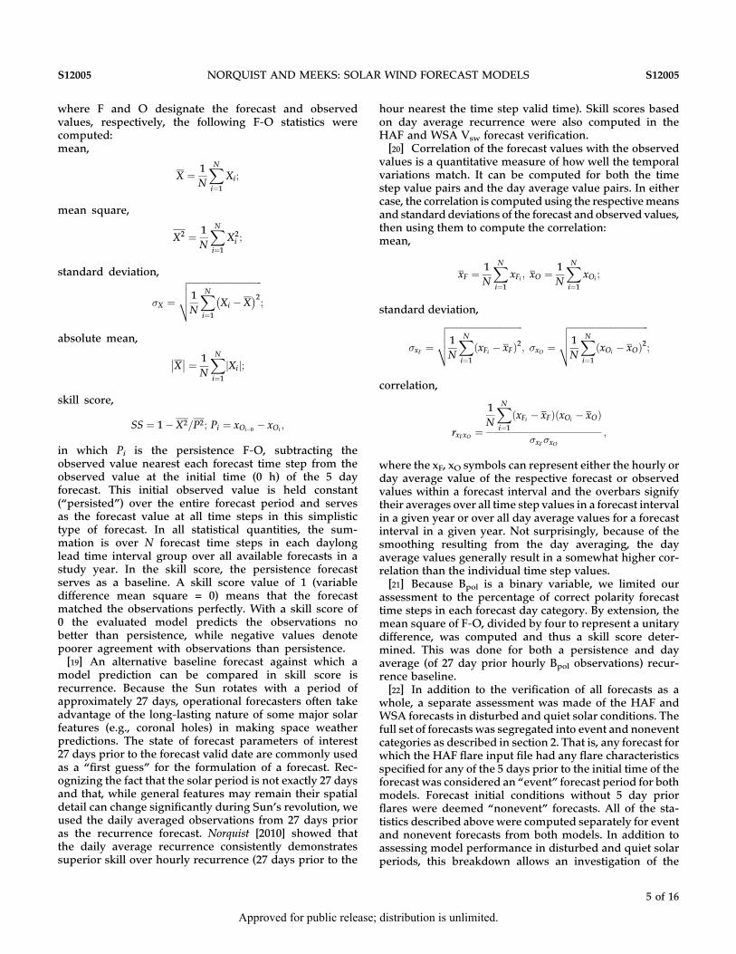
ences (F‐O) mean. To set the context, the observationalmean solar wind speed (Vsw) and magnitude of the mag-netic field vector ∣B∣ for the 6 study years are displayed inTable 1. In Solar Cycle 23 solar activity with regard tosunspot number reached a peak in mid‐2000 and stayedhigh until beginning to decline in early 2002 (NationalGeophysical Data Center, ftp://ftp.ngdc.noaa.gov/STP/SOLAR_DATA/SUNSPOT_NUMBERS/AMERICAN/, seeSMOOTHED.PLT for smoothed monthly mean sunspotnumber). Both 1997 and 2007 were solar minimum years,1999 was in the ascending phase and 2003 and 2005 werein the declining phase. To minimize systematic error theforecast models must reproduce the climatology of thesolar wind so that the annual F‐O mean computed asdescribed in section 3 for each forecast day is small. Theyare shown in Figure 1 for the HAF and WSA forecasts. Infive of the years both models display a negative bias rel-ative to the observed mean. Even with the greaterobserved mean in 2003, as a percentage of the observedmean the F‐O mean is largest in 2003 for both models, asgreat as −21% for HAF and −14% for WSA. Anothernotable property of the F‐Omean is that the negative bias ofthe HAF forecast mean Vsw increases with increasingforecast lead time in five of the 6 years. This is only apparentin 3 years for WSA and to a much lesser extent. Theobserved mean (not shown) remains virtually unchangedwith forecast lead time as expected. The speed bias overall years and forecast days was −34 and −22 km s−1 for

Figure 1. Solar wind speed (Vsw) forecast‐observation difference (F‐O) mean (km s−1) for all HAFand WSA forecasts in each study year, computed separately for forecast days 1–5.


6 of 16


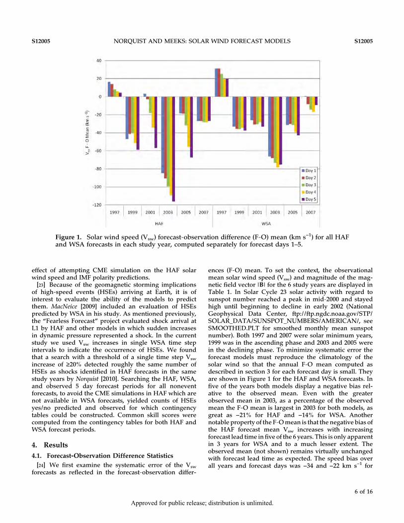
HAF andWSA, respectively, representing −8% and −5% ofthe overall observed mean Vsw.[25] The magnitude of the forecast departure from the

mean is represented by the F‐O absolute mean. This isshown as a percentage of the observed mean Vsw inFigure 2. By this metric, a measure of the ability of themodels to replicate the observations, HAF had its worseperformance in 2007 while WSA displayed somewhatsmaller F‐O in its worst years of 2001 and 2005. There isno indication of the growing slow bias of Vsw with leadtime for HAF in this graph. This indicates that it was dueto an increase in the number of negative F‐O time stepswith greater forecast lead time rather than the differencemagnitude growing larger at those time steps. This wasconfirmed with histograms of F‐O counts by discrete F‐Osize bins (not shown) showing an increasing numberof counts of the negative difference categories withincreasing forecast day. Vsw F‐O magnitude in the 6

study years as a percentage of the observed mean Vsw is20.3% for HAF and 17.8% for WSA.[26] Next we consider the random component of the

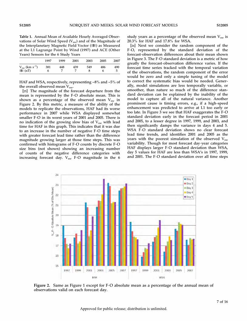
F‐O, represented by the standard deviation of theforecast‐observation differences about their mean shownin Figure 3. The F‐O standard deviation is a metric of howgreatly the forecast‐observation difference varies. If theforecast time series tracked with the temporal variationof the observations, the random component of the errorwould be zero and only a simple tuning of the modelto correct the systematic bias would be needed. Gener-ally, model simulations are less temporally variable, orsmoother, than nature so much of the difference stan-dard deviation can be explained by the inability of themodel to capture all of the natural variance. Anotherprominent cause is timing errors, e.g., if a high‐speedenhancement was predicted to arrive at L1 too early ortoo late. In Figure 3 we see that HAF exaggerates the F‐Ostandard deviation early in the forecast period in 2001and 2005, to a lesser degree in 1997, 1999, and 2003, andthen significantly damps the variance in days 4 and 5.WSA F‐O standard deviation shows no clear forecastlead time trends, and identifies 2001 and 2005 as theyears with the poorest simulation of the observed Vsw

variability. Though for most forecast day‐year categoriesHAF displays larger F‐O standard deviation than WSA,day 5 values for HAF are less than WSA’s in 1997, 1999,and 2001. The F‐O standard deviation over all time steps

Table 1. Annual Mean of Available Hourly Averaged Obser-vations of Solar Wind Speed (Vsw) and of the Magnitude ofthe Interplanetary Magnetic Field Vector (∣B∣) as Measuredat the L1 Lagrange Point by Wind (1997) and ACE (OtherYears) Sensors for the 6 Study Years

1997 1999 2001 2003 2005 2007

Vsw (km s−1) 381 448 439 549 486 490∣B∣ (nT) 6 7 7 8 6 5

Figure 2. Same as Figure 1 except for F‐O absolute mean as a percentage of the annual mean ofobservations valid on each forecast day.


7 of 16


in all years was 111.3 and 97.5 km s−1 in the HAF andWSA Vsw forecasts, respectively.[27] It was mentioned in the previous paragraph that

models usually underrepresent the temporal variance of aprognostic quantity. In the case of Vsw, this was examinedby evaluating the full standard deviation of Vsw asobserved and as predicted by HAF and WSA. When thestandard deviation was assessed separately by year and byforecast day, the latter showed a significant decline fromday 1 to day 5 in the HAF forecasts. Figure 4 indicates thatHAF forecasts begin with a standard deviation similar tothat of observations, which is then severely damped beloweven WSA’s that is consistently less than observed. Thisresult is consistent with the excessive F‐O standarddeviations early in HAF forecasts in Figure 3. That is,when standard deviations of both HAF and observationsare large, the difference standard deviations are likely tobe large as well. The overall Vsw standard deviation forHAF, WSA, and observations is 88.1, 78.9, and 98.8 km s−1,respectively. The latter two values compare with 84.3 forWSA and 99.2 km s−1 for observations as computed byOwens et al. [2008] for 1995–2002.[28] The day average forecast and observed means and

standard deviations were used to compute the day aver-age forecast versus observation correlations shown inFigure 5. The forecast day average correlations are slightlyhigher than their single time step counterparts in allforecast day‐year categories for both models. Figure 5indicates that there is significant variation in the correla-tions among the study years, from values less than 0.2 in

2001 to values above 0.5 in 2003 for both models. The year‐to‐year change is the same for the models until 2007, whenthe HAF correlations are smallest and WSA’s are secondto largest. This is consistent with the relative values of F‐Ostandard deviation in 2007 as seen in Figure 3. Over allyears and forecast days, the day‐average Vsw correlationsare 0.32 and 0.42 for HAF and WSA, respectively.[29] We now turn our attention to skill score of the Vsw

forecasts. Table 2 presents the skill score values withrespect to persistence and recurrence for all forecast day‐year categories. The results indicate that, except for earlyin the forecast period (day 1 and for the first 4 years day 2),recurrence is a higher standard as a reference for modelforecasts than is persistence. Persistence is expected tobeat either model or recurrence in the first forecast daysince on many days Vsw changes slowly. However,recurrence excels over persistence in skill (i.e., the modelshave a more negative score with respect to recurrence) byday 2 or 3. In fact, as the values in Table 2 indicate,recurrence is superior in skill (i.e., show a negative skillscore) to the models on days 4 and 5 in all years for HAFand 3 years for WSA, whereas both models beat persis-tence on those days in all but one forecast day‐year cate-gory. Except for 1997, WSA skill scores are greater thanHAF’s with respect to both references in all of the forecastday‐year categories. In regards to recurrence skill score,it is clear from Table 2 that neither model shows anydiscernable Vsw prediction improvement or degradationtrend with forecast lead time. The WSA persistence‐basedskill scores computed by MacNeice [2009] for MWO initial

Figure 3. Same as Figure 1 except for F‐O standard deviation.


8 of 16


Figure 5. Correlations of day average HAF and WSA Vsw forecasts with day average observationsin each study year, computed separately for forecast days 1–5.

Figure 4. Standard deviation of HAF and WSA Vsw forecasts and observations (Obs) computedover all study years by forecast day.


9 of 16


conditions and 5.0 Rs source surface were −1.19, −0.16, and0.18 for days 1, 2, and 4. In comparison, the correspondingWSA skill scores computed in this study for the sameforecast days over all study years were −2.5, −0.07, and0.39. The significantly better performance of day 1 per-sistence over WSA in the current study may be due to

using the observed value at the 0 h of the forecastthroughout the first day, rather than the 24 h earlier valueat each forecast time step as was done by MacNeice [2009].[30] The comparative performance of the two models in

predicting Bpol at L1 is first displayed as the percentage ofcorrect forecasts as shown in Figure 6. The pattern of

Table 2. Vsw Skill Scores With Respect to Persistence (Per) and Recurrence (Rec) for All Forecast Day‐Year Categories in ThisStudy

HAF WSA

Day 1 Day 2 Day 3 Day 4 Day 5 Day 1 Day 2 Day 3 Day 4 Day 5

1997Per −5.57 −0.89 −0.09 0.09 0.12 −5.15 −0.91 −0.20 −0.01 0.05Rec −0.43 −0.24 −0.09 −0.13 −0.18 −0.34 −0.26 −0.21 −0.25 −0.28

1999Per −2.90 −0.47 0.10 0.27 0.29 −2.19 −0.12 0.19 0.33 0.37Rec −0.03 −0.13 0.01 −0.01 −0.10 0.16 0.14 0.11 0.07 0.03

2001Per −5.30 −0.88 0.09 0.09 0.11 −2.07 −0.09 0.12 0.17 0.20Rec −0.90 −0.65 0.00 −0.11 −0.24 0.07 0.05 0.03 −0.02 −0.11

2003Per −3.89 −0.56 0.00 0.12 0.12 −2.21 0.00 0.29 0.38 0.45Rec −0.33 −0.46 −0.39 −0.38 −0.45 0.12 0.07 0.01 0.02 0.10

2005Per −4.26 −0.73 0.16 0.39 0.47 −2.12 −0.02 0.30 0.50 0.56Rec −0.75 −0.73 −0.23 −0.17 −0.06 −0.04 −0.02 −0.03 0.03 0.12

2007Per −5.03 −0.47 0.13 0.31 0.36 −2.75 0.14 0.45 0.56 0.61Rec −0.92 −1.01 −1.03 −1.10 −1.10 −0.20 −0.18 −0.29 −0.32 −0.30

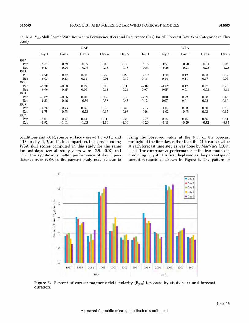
Figure 6. Percent of correct magnetic field polarity (Bpol) forecasts by study year and forecastduration.


10 of 16


performance by year is same for both models, and theactual values are similar, too. In all years and forecastdays, the percent of correct Bpol forecasts is virtually thesame for HAF and WSA, 72.7% and 72.6%, respectively. Itis interesting to note that in the year with the largest IMFmagnitude, 2003, the percentage of correct forecasts byboth models is 10%–15% greater than the other years.Norquist [2010] also found that skill in predicting themagnetic field vector azimuth angle (the angle the vectormakes with the Sun‐Earth line when projected on theecliptic plane) was much better predicted in 2003 by HAFthan for the other years. MacNeice [2009] found thatthe same configuration of WSA using MWO magneto-grams produced Bpol predictions that match observationsin 76% of the forecast times.[31] The final comparative metric for the Bpol forecasts is

skill score. Both persistence and day average recurrencewere used as the reference as was done for the Vsw fore-casts. Table 3 shows the skill score values for all forecastyear categories. As was the case for Vsw, recurrence fore-casts are tougher for the models to beat than persistence.But in Bpol, this begins with day 1 as evidenced by thelarger negative values at all 5 days in a majority of theyears for both models. As was seen in the percent ofcorrect Bpol forecasts in Figure 6, 2003 has the best Bpol

skill scores from both models with respect to persistence.However, there is no clear‐cut best year in regards torecurrence. In fact, neither model exceeds recurrence inskill, only in a single forecast day‐year category (1999‐1) inthe WSA predictions is the model better. Nor does eithermodel show any clear trend of forecast skill as a functionof forecast lead time with respect to recurrence. In fairnessto the models, the recurrence Bpol “forecast” value wascomputed as the average of the hourly observed −1 and

+1 values 27 days prior to the valid time forecast day. Assuch the average could have any value between the twopolarity values and thus would result in a lower F‐O meansquare than would result if a −1 or +1 value was imposedas the recurrence forecast. Persistence also did not havethat advantage, as a single value of Bpol (the 0 h observa-tion) was used. The mean square F‐O was computed overall forecast days and study years and was, from best toworst: Rec, 0.23; HAF, 0.27; WSA, 0.27; and Per, 0.49. Inother words, the Bpol forecasts from HAF and WSAexcelled over persistence but were inferior to recurrence.The WSA persistence‐based skill scores for Bpol com-puted in this study were somewhat better than those ofMacNeice [2009]: day 1, 2, and 4 values were −0.03, 0.21and 0.35 in the current study and −0.83, 0.01, and 0.04according to his evaluation.

4.2. Event Versus Nonevent Forecasts[32] HAF and WSA forecasts were also assessed sepa-

rately for event and nonevent 5 day forecast periods. Inevent forecasts, HAF inputs included flare properties forat least one flare event in the 5 days prior to forecastperiod start. These enabled HAF to simulate a CMEpropagating to L1 in accordance with the assumptionsdetailed by Fry et al. [2001]. In nonevent cases both modelsoperated in the absence of such disturbances. The numberof WSA forecast time steps, at which both models werecompared with observations in the respective conditions,are shown in Figure 7.[33] Space does not allow us to reproduce all of the F‐O

statistics charts of section 4.1 separated by event andnonevent forecasts. So we show the more telling aspects ofthe effects of disturbed versus quiet conditions on theforecasts of the two models. We begin with the standard

Table 3. Bpol Skill Scores With Respect to Persistence (Per) and Recurrence (Rec) for All Forecast Day‐Year Categories in ThisStudy

HAF WSA

Day 1 Day 2 Day 3 Day 4 Day 5 Day 1 Day 2 Day 3 Day 4 Day 5

1997Per 0.07 0.24 0.29 0.25 0.27 0.02 0.21 0.26 0.23 0.27Rec −0.14 −0.15 −0.11 −0.13 −0.19 −0.19 −0.19 −0.16 −0.17 −0.18

1999Per −0.08 0.21 0.30 0.34 0.42 −0.02 0.23 0.32 0.36 0.42Rec −0.01 −0.08 −0.07 −0.10 −0.12 0.04 −0.06 −0.04 −0.07 −0.14

2001Per −0.15 0.11 0.23 0.25 0.36 −0.10 0.19 0.23 0.26 0.30Rec −0.17 −0.26 −0.14 −0.15 −0.14 −0.12 −0.15 −0.13 −0.14 −0.23

2003Per 0.01 0.29 0.45 0.59 0.66 0.15 0.36 0.53 0.59 0.69Rec −0.21 −0.21 −0.17 −0.07 −0.07 −0.05 −0.09 −0.01 −0.09 0.00

2005Per −0.16 0.15 0.36 0.48 0.48 −0.23 0.14 0.31 0.40 0.46Rec −0.25 −0.22 −0.20 −0.08 −0.25 −0.32 −0.23 −0.30 −0.25 −0.29

2007Per 0.02 0.17 0.30 0.33 0.34 0.03 0.19 0.29 0.32 0.34Rec −0.32 −0.41 −0.35 −0.39 −0.37 −0.32 −0.38 −0.37 −0.39 −0.37


11 of 16


deviation of the Vsw forecasts and observations as shownin Figure 8. These results make it clear that all of thedramatic drop in standard deviation of HAF Vsw forecastsseen in Figure 4 is due to the event forecasts. In the first2 days of predictions HAF Vsw standard deviation exceedseven those observed. They drop down to a level that isreplicated in all 5 days of the nonevent forecasts. The latteris surprisingly similar to that of the WSA forecasts indisturbed conditions but lower than the standard devia-tion of WSA forecasts in quiet conditions. As is seen inFigure 4, both models’ variance is well below that of theobservations in either of the conditions after the severedamping in the HAF event forecasts.[34] As one would suspect from this result, almost all of

the F‐O mean decrease with forecast day in HAF predic-tions (Figure 1) was due to the event forecasts (not shown).This was also true of the HAF Vsw F‐O standard deviationsfrom event forecasts (not shown) in which the days 1 and 2values are greater than 160 km s−1 in 2005 (compare withFigure 3 for all forecasts). The profile and magnitude of theWSA nonevent Vsw F‐O standard deviations look verymuch like those of Figure 3 for all forecasts while for theevent forecasts the years at and after solar maximum(2001–2005) have the largest values. WSA event forecastshad somewhat larger F‐O standard deviations than did the

nonevent cases unlike the forecast Vsw standard devia-tions in Figure 8. The WSA event and nonevent Vsw skillscores were very much alike.[35] In regards to Bpol prediction performance in event

and nonevent forecasts, we found that they were better innonevent periods in all study years but one. This is seen inFigure 9, which shows the percent of correct Bpol forecastsover all forecast days for each study year. Uncertainty isgreatest in event forecasts of 1997 and 2007 due to therelatively few forecast time steps used in the verificationas seen in Figure 7. In agreement with the results overboth disturbed and quiet conditions shown in Figure 6,2003 was the best year for both models in both conditions,due perhaps in part to the greater number of noneventthan event verification time steps (Figure 7). By contrast, in2001 when event forecasts dominate, there are fewer cor-rect Bpol forecasts (Figure 6) and the contrast betweenevent and nonevent skill is greatest (Figure 9).

4.3. High‐Speed Event Analysis[36] We examined both models’ forecasts and the

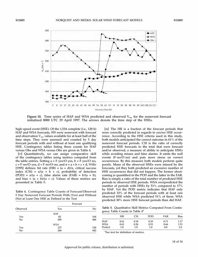
observations in all of the nonevent 5 day forecast periodsfor single (4.55 h) time step Vsw increases of 20%. InFigure 10 we show a forecast period beginning on 29April 1997 at 0000 UTC in which all three had such a

Figure 7. Number of forecast time steps used in the verification of event and nonevent forecastsfor each forecast day and year for both Vsw and Bpol forecasts.


12 of 16


Figure 9. Percent of correct Bpol forecasts for HAF and WSA event and nonevent forecast periodsover all forecast days by study year.

Figure 8. Standard deviation of HAF, WSA, and observed Vsw computed separately for event andnonevent forecasts over all study years by forecast day.


13 of 16


high‐speed event (HSE). Of the 1,534 complete (i.e., 120 h)HAF and WSA forecasts, 935 were nonevent with forecastand observation Vsw values available for at least half of thetime steps. They were assessed and counted by 5 dayforecast periods with and without at least one qualifyingHSE. Contingency tables listing these counts for HAFversus Obs and WSA versus Obs are given in Table 4.[37] Quantitatively, we can assign comparative skill

of the contingency tables using metrics computed fromthe table entries. Setting a = F‐yes/O‐yes, b = F‐yes/O‐no,c = F‐no/O‐yes, d = F‐no/O‐no, and n = a + b + c + d,Wilks[1995] defines: hit rate (HR) = (a + d)/n, critical successindex (CSI) = a/(a + b + c), probability of detection(POD) = a/(a + c), false alarm rate (FAR) = b/(a + b),and bias = (a + b)/(a + c). Values of these metrics arepresented in Table 5.

[38] The HR is a fraction of the forecast periods thatwere correctly predicted in regards to yes/no HSE occur-rence. According to the HSE criteria used in this study,both models anticipated the correct outcome in 61% of thenonevent forecast periods. CSI is the ratio of correctlypredicted HSE forecasts to the total that were forecastand/or observed, a measure of ability to anticipate HSEswhile avoiding misses and false alarms. It omits the nullevents (F‐no/O‐no) and puts more stress on correctoccurrences. By this measure both models perform quitepoorly. Many of the observed HSEs were missed by theforecasts, yet they both predicted an excessive number ofHSE occurrences that did not happen. The former short-coming is quantified in the POD and the latter in the FAR.Bias is simply a ratio of the total number of predicted HSEperiods to observed HSE periods. WSA overpredicted thenumber of periods with HSEs by 51% compared to 17%by HAF. Yet the POD metric indicates that HAF onlypredicted 33% of the forecast periods with at least oneobserved HSE while WSA predicted 51% of them. WSApredicted 30% more HSE forecast periods than did HAF.

Table 5. Quantitative Skill Metrics Computed From Contin-gency Table Counts in Table 4a

HR CSI POD FAR Bias

HAF 0.61 0.18 0.33 0.71 1.17WSA 0.61 0.26 0.51 0.66 1.51Perfect 1.0 1.0 1.0 0.0 1.0

aSee text for definition of metrics.

Table 4. Contingency Table Counts of Forecast/Observed5 Day Nonevent Forecast Periods With (Yes) and Without(No) at Least One HSE as Defined in the Text

Observed

Forecast

Yes No

HAFYes 82 164No 205 484

WSAYes 127 120No 246 442

Figure 10. Time series of HAF and WSA predicted and observed Vsw for the nonevent forecastinitialized 0000 UTC 29 April 1997. The arrows denote the time step of the HSEs.


14 of 16


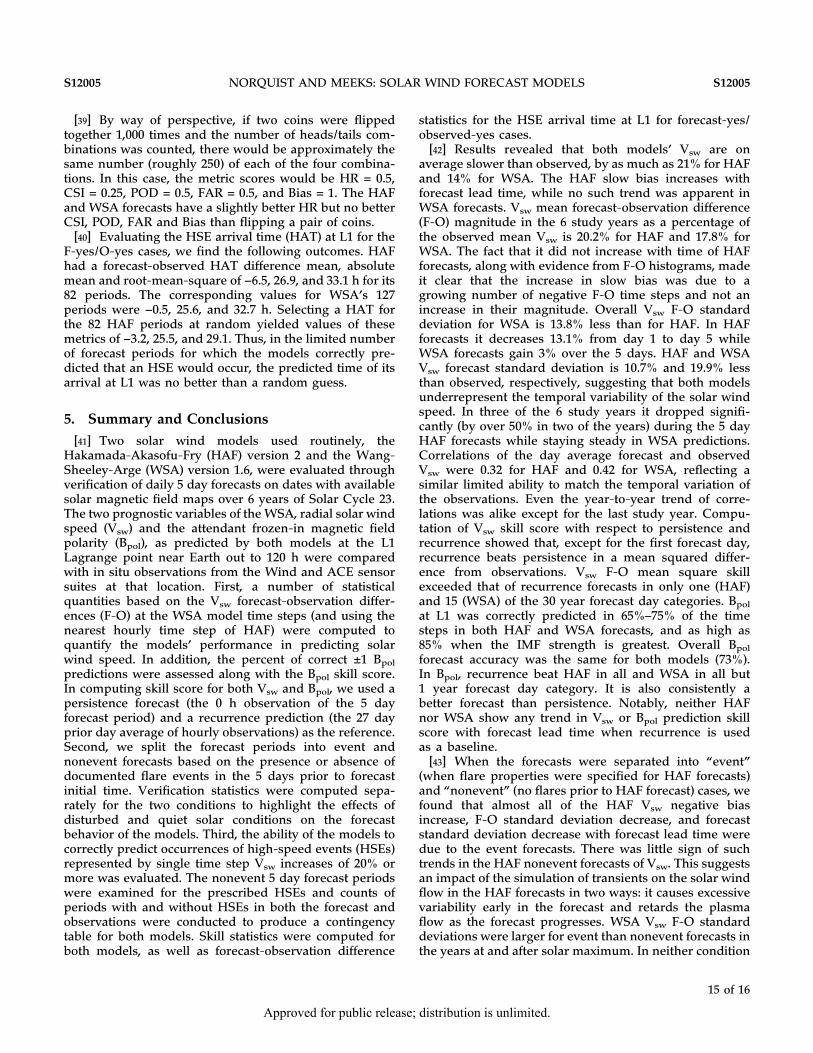
[39] By way of perspective, if two coins were flippedtogether 1,000 times and the number of heads/tails com-binations was counted, there would be approximately thesame number (roughly 250) of each of the four combina-tions. In this case, the metric scores would be HR = 0.5,CSI = 0.25, POD = 0.5, FAR = 0.5, and Bias = 1. The HAFand WSA forecasts have a slightly better HR but no betterCSI, POD, FAR and Bias than flipping a pair of coins.[40] Evaluating the HSE arrival time (HAT) at L1 for the

F‐yes/O‐yes cases, we find the following outcomes. HAFhad a forecast‐observed HAT difference mean, absolutemean and root‐mean‐square of −6.5, 26.9, and 33.1 h for its82 periods. The corresponding values for WSA’s 127periods were −0.5, 25.6, and 32.7 h. Selecting a HAT forthe 82 HAF periods at random yielded values of thesemetrics of −3.2, 25.5, and 29.1. Thus, in the limited numberof forecast periods for which the models correctly pre-dicted that an HSE would occur, the predicted time of itsarrival at L1 was no better than a random guess.

5. Summary and Conclusions[41] Two solar wind models used routinely, the

Hakamada‐Akasofu‐Fry (HAF) version 2 and the Wang‐Sheeley‐Arge (WSA) version 1.6, were evaluated throughverification of daily 5 day forecasts on dates with availablesolar magnetic field maps over 6 years of Solar Cycle 23.The two prognostic variables of theWSA, radial solar windspeed (Vsw) and the attendant frozen‐in magnetic fieldpolarity (Bpol), as predicted by both models at the L1Lagrange point near Earth out to 120 h were comparedwith in situ observations from the Wind and ACE sensorsuites at that location. First, a number of statisticalquantities based on the Vsw forecast‐observation differ-ences (F‐O) at the WSA model time steps (and using thenearest hourly time step of HAF) were computed toquantify the models’ performance in predicting solarwind speed. In addition, the percent of correct ±1 Bpol

predictions were assessed along with the Bpol skill score.In computing skill score for both Vsw and Bpol, we used apersistence forecast (the 0 h observation of the 5 dayforecast period) and a recurrence prediction (the 27 dayprior day average of hourly observations) as the reference.Second, we split the forecast periods into event andnonevent forecasts based on the presence or absence ofdocumented flare events in the 5 days prior to forecastinitial time. Verification statistics were computed sepa-rately for the two conditions to highlight the effects ofdisturbed and quiet solar conditions on the forecastbehavior of the models. Third, the ability of the models tocorrectly predict occurrences of high‐speed events (HSEs)represented by single time step Vsw increases of 20% ormore was evaluated. The nonevent 5 day forecast periodswere examined for the prescribed HSEs and counts ofperiods with and without HSEs in both the forecast andobservations were conducted to produce a contingencytable for both models. Skill statistics were computed forboth models, as well as forecast‐observation difference

statistics for the HSE arrival time at L1 for forecast‐yes/observed‐yes cases.[42] Results revealed that both models’ Vsw are on

average slower than observed, by as much as 21% for HAFand 14% for WSA. The HAF slow bias increases withforecast lead time, while no such trend was apparent inWSA forecasts. Vsw mean forecast‐observation difference(F‐O) magnitude in the 6 study years as a percentage ofthe observed mean Vsw is 20.2% for HAF and 17.8% forWSA. The fact that it did not increase with time of HAFforecasts, along with evidence from F‐O histograms, madeit clear that the increase in slow bias was due to agrowing number of negative F‐O time steps and not anincrease in their magnitude. Overall Vsw F‐O standarddeviation for WSA is 13.8% less than for HAF. In HAFforecasts it decreases 13.1% from day 1 to day 5 whileWSA forecasts gain 3% over the 5 days. HAF and WSAVsw forecast standard deviation is 10.7% and 19.9% lessthan observed, respectively, suggesting that both modelsunderrepresent the temporal variability of the solar windspeed. In three of the 6 study years it dropped signifi-cantly (by over 50% in two of the years) during the 5 dayHAF forecasts while staying steady in WSA predictions.Correlations of the day average forecast and observedVsw were 0.32 for HAF and 0.42 for WSA, reflecting asimilar limited ability to match the temporal variation ofthe observations. Even the year‐to‐year trend of corre-lations was alike except for the last study year. Compu-tation of Vsw skill score with respect to persistence andrecurrence showed that, except for the first forecast day,recurrence beats persistence in a mean squared differ-ence from observations. Vsw F‐O mean square skillexceeded that of recurrence forecasts in only one (HAF)and 15 (WSA) of the 30 year forecast day categories. Bpol

at L1 was correctly predicted in 65%–75% of the timesteps in both HAF and WSA forecasts, and as high as85% when the IMF strength is greatest. Overall Bpol

forecast accuracy was the same for both models (73%).In Bpol, recurrence beat HAF in all and WSA in all but1 year forecast day category. It is also consistently abetter forecast than persistence. Notably, neither HAFnor WSA show any trend in Vsw or Bpol prediction skillscore with forecast lead time when recurrence is usedas a baseline.[43] When the forecasts were separated into “event”

(when flare properties were specified for HAF forecasts)and “nonevent” (no flares prior to HAF forecast) cases, wefound that almost all of the HAF Vsw negative biasincrease, F‐O standard deviation decrease, and forecaststandard deviation decrease with forecast lead time weredue to the event forecasts. There was little sign of suchtrends in the HAF nonevent forecasts of Vsw. This suggestsan impact of the simulation of transients on the solar windflow in the HAF forecasts in two ways: it causes excessivevariability early in the forecast and retards the plasmaflow as the forecast progresses. WSA Vsw F‐O standarddeviations were larger for event than nonevent forecasts inthe years at and after solar maximum. In neither condition


15 of 16


did they show any trend with forecast lead time as didHAF in Vsw event forecasts. Both models demonstratedsomewhat higher Bpol prediction skill in nonevent thanevent forecasts.[44] Single model time step increases of 20% or more in

Vsw, the criterion used to denote HSEs, were analyzed inthe 5 day nonevent forecast periods for both models andobservations. Both models produced an excessive numberof forecasts with HSEs. More of the forecast periods withobserved HSEs were missed by HAF than were predicted,while WSA predicted about half of them. Neither modeldemonstrated any skill above a random guess in regardsto predicting the HSE arrival time at L1 in forecast periodswith predicted and observed HSEs. These results suggestthat there is a lot of room for improvement in the pre-diction of high‐speed streams and corotating interactionregions.[45] In summary, the WSA model performed somewhat

better in Vsw prediction than HAF, whereas they wereabout even in Bpol skill. HAF Vsw event forecasts weresubject to decreasing speed throughout the integrationand excessive variance earlier in the forecast period thatwas damped below that of HAF by day 5. In quiet solarconditions both models underrepresent the temporalvariability of the observed Vsw. Recurrence still remains abetter forecast than what can be produced by the modelsespecially in magnetic field polarity. These findingsaccentuate the challenges involved in the realistic simu-lation of the solar wind and its attendant magnetic field.Future evaluations of more advanced physics modelsshould shed light on how their performance varies withforecast lead time and solar activity level.

[46] Acknowledgments. We thank Ghee Fry of ExplorationPhysics, Inc. for his guidance in setting up and executing the HAFmodel, as well as for providing the event files listing the specificationof flare properties. We express our appreciation to our colleague NickArge for providing the WSA model code, the MWO magnetic fieldmap files, and the Wind/ACE observations. The WIND satellite datawere originally obtained from Massachusetts Institute of TechnologySpace Plasma Group and National Aeronautics and Space Adminis-tration, and the ACE data were obtained from the ACE Science Cen-ter at California Institute of Technology. Funding for the secondauthor was provided by the Space Vehicles Directorate Space Scho-lars program. Overall funding and support for this project was pro-vided by the applied research program and the Space WeatherForecasting Laboratory of the Air Force Research Laboratory.

ReferencesAltschuler, M. D., and G. Newkirk (1969), Magnetic fields and thestructure of the solar corona. I: Methods of calculating coronalfields, Sol. Phys., 9, 131–149, doi:10.1007/BF00145734.

Arge, C. N., and V. J. Pizzo (2000), Improvements in the prediction ofsolar wind conditions using near‐real time solar magnetic field up-dates, J. Geophys. Res., 105, 10,465–10,480, doi:10.1029/1999JA000262.

Arge, C. N., J. G. Luhmann, D. Odstrcil, C. J. Schrijver, and Y. Li(2004), Stream structure and coronal sources of the solar wind dur-ing the May 12th, 1997 CME, J. Atmos. Sol. Terr. Phys., 66, 1295–1309,doi:10.1016/j.jastp.2004.03.018.

Fry, C. D., W. Sun, C. S. Deehr, M. Dryer, Z. Smith, S.‐I. Akasofu,M. Tokumaru, and M. Kojima (2001), Improvements to the HAFsolar wind model for space weather predictions, J. Geophys. Res.,106, 20,985–21,001, doi:10.1029/2000JA000220.

Fry, C. D., M. Dryer, Z. Smith, W. Sun, C. S. Deehr, and S.‐I. Akasofu(2003), Forecasting solar wind structures and shock arrival timesusing an ensemble of models, J. Geophys. Res., 108(A2), 1070,doi:10.1029/2002JA009474.

Lee, C. O., J. G. Luhmann, D. Odstrcil, P. J. MacNeice, I. de Pater,P. Riley, and C. N. Arge (2009), The solar wind at 1 AU duringthe declining phase of Solar Cycle 23: Comparison of 3D numer-ical model results with observations, Sol. Phys., 254, 155–183,doi:10.1007/s11207-008-9280-y.

Linker, J. A., Z. Mikić, D. A. Biesecker, R. J. Forsyth, S. E. Gibson, A. J.Lazurus, A. Lecinski, P. Riley, A. Szabo, and B. J. Thompson (1999),Magnetohydrodynamic modeling of the solar corona during WholeSun Month, J. Geophys. Res. , 104 , 9809–9830, doi:10.1029/1998JA900159.

MacNeice, P. (2009), Validation of community models: 2. Develop-ment of a baseline using the Wang‐Sheeley‐Arge model, SpaceWeather, 7, S12002, doi:10.1029/2009SW000489.

McKenna‐Lawlor, S. M. P., M. Dryer, M. D. Kartalev, Z. Smith, C. D.Fry, W. Sun, C. S. Deehr, K. Kecskemety, and K. Kudela (2006),Near real‐time predictions of the arrival at Earth of flare‐relatedshocks during Solar Cycle 23, J. Geophys. Res., 111, A11103,doi:10.1029/2005JA011162.

Mikić, Z., J. A. Linker, D. D. Schnack, R. Lionello, and A. Tarditi(1999), Magnetohydrodynamic modeling of the global solar corona,Phys. Plasmas, 6, 2217–2224, doi:10.1063/1.873474.

Norquist, D. C. (2010), Verification of forecasts from the Hakamada‐Akasofu‐Fry v2 solar wind model, Rep. AFRL‐RV‐HA‐TR‐2010‐1010,69 pp., Air Force Res. Lab., Air Force Mater. Command, HanscomAir Force Base, Mass.

Odstrcil, D. (2003), Modeling 3‐D solar wind structures, Adv. SpaceRes., 32, 497–506, doi:10.1016/S0273-1177(03)00332-6.

Owens, M. J., H. E. Spence, S. McGregor, W. J. Hughes, J. M. Quinn,C. N. Arge, P. Riley, J. Linker, and D. Odstrcil (2008), Metrics forsolar wind prediction models: Comparison of empirical, hybrid,and physics‐based schemes with 8 years of L1 observations, SpaceWeather, 6, S08001, doi:10.1029/2007SW000380.

Schatten, K. H. (1971), Current sheet magnetic model for the solarcorona, Cosmic Electrodyn., 2, 232–245.

Smith, Z. K., M. Dryer, S. M. P. McKenna‐Lawlor, C. D. Fry, C. S.Deehr, and W. Sun (2009), Operational validation of HAFv2’s pre-dictions of interplanetary shock arrivals at Earth: Declining phaseof Solar Cycle 23, J. Geophys. Res., 114, A05106, doi:10.1029/2008JA013836.

Wilks, D. S. (1995), Statistical Methods in the Atmospheric Sciences,467 pp., Academic, San Diego, Calif.

W. C. Meeks and D. C. Norquist, Battlespace EnvironmentDivision, Space Vehicles Directorate, Air Force ResearchLaboratory, Hanscom Air Force Base, MA 01731, USA. ([email protected])


16 of 16


DISTRIBUTION LIST

DTIC/OCP 8725 John J. Kingman Rd, Suite 0944 Ft Belvoir, VA 22060-6218 1 cy AFRL/RVIL Kirtland AFB, NM 87117-5776 2 cys Official Record Copy AFRL/RVBXS/Donald Norquist 1 cy


This page intentionally left blank.


a comparative verification of forecasts from · pdf filea comparative verification of...

Documents