A Comparison of Formulations and Relaxations for Cross-dock

Door Assignment Problems

W. Nassiefa, I. Contrerasa, B. Jaumardb,∗

aConcordia University and Interuniversity Research Centre on Enterprise Networks, Logistics andTransportation (CIRRELT), Montreal, Canada H3G 1M8

bConcordia University, Computer Science and Software Engineering Department, Montreal, Canada H3G1M8

Abstract

This paper deals with cross-dock door assignment problems in which the assignments ofincoming trucks to strip doors, and outgoing trucks to stack doors are determined, with theobjective of minimizing the total handling cost. We present two new mixed integer program-ming formulations which are theoretically and computationally compared with existing ones.One of such requires a column generation algorithm to solve its associated linear relaxation.We present the results of a series of computational experiments to evaluate the performanceof the formulations on a set of benchmark instances. We also perform sensitivity analysiswith respect to several input parameters of the Cross-dock Door Assignment Problems.

Keywords: cross-docking, MIP formulations, relaxations and bounds, column generation

1. Introduction

Cross-docking is a logistic strategy that facilitates rapid movement of consolidated prod-ucts between suppliers and retailers within a supply chain. It is also a warehousing strategythat aims at reducing or eliminating storage and order picking, two of which are known tobe major costly operations of any typical warehouse. This strategy has been used in the5

retailing, manufacturing, automotive, and photographic industries, and has been successfullyimplemented by several companies such as Walmart and Toyota. For examples of successfulcross-docking implementations, the interested reader is referred to Forger (1995), Kinnear(1997), Witt (1998), Chen and Song (2009), and Napolitano (2011).

Cross-dock facilities (or cross-docks) are designed to expedite the movement of highly10

and constantly demanded materials, which eventually lead to a better service level andquicker response across the supply chain at a reduced cost. Particularly, once incoming andoutgoing trucks are assigned to their designated doors, the goods get unloaded from theincoming trucks, consolidated in a staging area according to their destinations, and loadedinto the outgoing trucks with minimal storage in between. In practice, minimal storage is15

possible, and so, it comes in different forms that can range from temporary buffers in front

∗corresponding authorEmail addresses: wael.nassief@cirrelt.ca (W. Nassief), ivan.contreras@cirrelt.ca (I.

Contreras), bjaumard@cse.concordia.ca (B. Jaumard)

Preprint submitted to Computers & Operations Research November 23, 2017

of the doors to even a designated temporary storage area. Typically, the amount of timegoods spend at a cross-dock ranges from virtually none to about 24 hours. The variousadvantages of cross-docking as compared to the different practices of traditional warehousesand point-to-point deliveries are listed in Van Belle et al. (2012).20

Given the inherent complexity of designing and operating cross-docks, several classesof decision problems have been studied in the literature. Agustina et al. (2010), Boysen(2010), Shuib and Fatthi (2012), Van Belle et al. (2012), and Buijs et al. (2014) providereviews of decision problems arising in cross-docking. Moreover, a recent review by Ladierand Alpan (2016) proposes a framework that highlights the gaps between the literature and25

some cross-docking practices in France.In this paper we focus on a class of operational problems called cross-dock door assign-

ment problems (CDAPs), as referred to in Zhu et al. (2009), Guignard et al. (2012) andNassief et al. (2016). On a daily basis, fully loaded incoming trucks arrive to the cross-dockfacility. When docked (or assigned) to strip (inbound) doors, they get unloaded by em-30

ployees who inspect and sort the shipments according to their destinations. Using materialhandling equipment such as carts, forklifts or a system of conveyors, these shipments aretransferred to some stack (outbound) doors ready for loading into outgoing trucks, whichare assigned according to their destinations. The material handling equipment keep travel-ing between strip and stack doors till all products are transferred to their designated stack35

doors. Then, employees load them into outgoing trucks. Whenever an outgoing truck isfilled with all needed products for its designated destination, it leaves the facility carryingthe consolidated products. CDAPs seek to optimally decide on the assignment of both in-coming trucks to strip doors and outgoing trucks to stack doors such that the total handlingcost inside the cross-dock is minimized. The assignment decisions affect the total time of40

getting shipments unloaded, traveled across the facility, and loaded. The cost is commonlymeasured as traveling distance between doors and thus, the objective needs only to focuson the weighted travel time between doors. Tsui and Chang (1990, 1992), Oh et al. (2006),Bozer and Carlo (2008), Cohen and Keren (2009), Zhu et al. (2009), Guignard et al. (2012),and Nassief et al. (2016) study CDAPs with this type of objective. However, in practice45

unloading and loading times do need to be taken into account, specially when these dependon the number and skill-level of workers assigned to each door. This is particularly relevantin applications where turnovers are very high (see, for instance Amini et al., 2014) and thus,there is a learning curve to be taken into account when unloading and loading. To the best ofour knowledge, there are only two works explicitly considering unloading and loading times50

at doors. Peck (1983) incorporates unloading and loading times along with travel times ascapacity constraints. Zhang et al. (2010) introduce these terms in one objective function inthe context of truck scheduling. The authors report on the impact of considering one termat a time versus all terms in a single objective function. We refer to Nassief et al. (2016) fora detailed literature review on CDAPs and Gelareh et al. (2016), and Enderer et al. (2017),55

Maknoon and Laporte (2017) and Maknoon et al. (2017) for recent extensions of CDAPs inwhich additional operational decisions are considered.

In this paper we study the standard CDAP considered in Zhu et al. (2009), Guignard et al.(2012), and Nassief et al. (2016) and show how door-dependent unloading and loading costscan be easily integrated in the objective, in addition to the transfer costs between doors. We60

assume workforce assignment decisions to be exogenous, i.e., they are not part of the decision

2

process. From now on, we refer to this problem as the cross-dock door assignment problem(CDAP). Given the inherent complexity of the quadratic nature of CDAPs, most of theprevious studies have resorted to heuristic algorithms for their solution. However, little workhas been done for the study and development of mathematical programming formulations65

that can be solved with general purpose solvers or embedded into decomposition techniques.The main contribution of this work is to study several mixed integer programming (MIP)formulations for the CDAP and to report on their performance. In particular, we present twonew MIP formulations which are theoretically and computationally compared with existingformulations of the CDAP. The formulations are compared with respect to the quality of their70

linear programming (LP) relaxation bounds and with respect to the Lagrangean relaxationintroduced in Nassief et al. (2016). Due to the huge number of variables involved in one of thenew formulations, we implement a column generation algorithm to solve its LP relaxation.Finally, we present the results of a series of computational experiments to evaluate therelative performance of the proposed and existing formulations and of the decomposition75

algorithms. As will be shown, although some formulations provide the same theoreticalbound, the convergence of their solution scheme may vary significantly.

The remainder of this paper is structured as follows. Section 2 provides a formal def-inition of the CDAP. In Section 3, we introduce several linear MIP formulations. Section4 presents the theoretical comparisons of the bounds provided by their LP relaxations and80

the Lagrangean relaxation of Nassief et al. (2016). In Section 5, we introduce the columngeneration algorithm used to solve one of the MIP formulations. Computational experimentsusing a set of benchmark instances are presented in Section 6. Conclusions follow in Section7.

2. Problem Statement85

Let M , N , I, and J denote the sets of origins, destinations, inbound and outbounddoors, respectively. The traveling time (or distance) between strip door i and stack door jis denoted by tij. Let ui and `j denote the per unit unloading and loading times for inbounddoor i and outbound door j, respectively. Unloading and loading times vary by doors sinceeach door has a designated employee with a skill level (e.g., from a beginner to a well trained90

employee). This is a common practice specially for cross-docks with third party contractorswhere employees are hired as needed. Moreover, well trained employees are allowed to useadvanced material handling equipment such as forklifts instead of trailers, which also affectthe unloading and loading times. The loading process is considered more time consumingthan the unloading one since it involves more steps and double handling. For instance,95

verifying the destination of the consolidated products, and making sure that outgoing trucksare fully loaded are additional steps compared to unloading. Let wmn be the amount ofcommodity originated at m and destined to n. Without loss of generality, the values wmncan be stated in terms of the number of times the material handling equipment (i.e., forklift,pallet jack, etc) needs to be used to transfer all the flow originated at m with destination100

n between a pair of strip/stack doors. For each m ∈ M , let sm =∑

n∈N wmn > 0 denotethe total supplied flow from an origin whereas for each n ∈ N , let rn =

∑m∈M wmn > 0

be the total sent flow towards a destination. We denote by Si and Rj the capacity forinbound door i ∈ I and outbound door j ∈ J , respectively. This capacity represents the

3

limit on the amount of commodities that the workforce and material handling equipment105

designated to each door can process in a given shift. These capacities are calculated bydividing the total amount of commodities coming to (or leaving from) the cross-dock by thetotal number of inbound (or outbound) doors, and then adding some capacity slackness.That is:

∑m∈M wmn/|I| ∗ slack, or by analogy it is the same to say

∑n∈N wmn/|J | ∗ slack.

The generation mechanism of all these parameters is detailed in Section 6.1.110

The CDAP consists of assigning each origin and each destination to exactly one inbounddoor and one outbound door, respectively, such that the capacity restrictions on dock doorsare satisfied and the total handling cost (unloading, transfer and loading) inside the cross-dock is minimum.

Given that each commodity has to pass through exactly one inbound and one outbound115

door, origin/destination paths are of the form (m, i, j, n), where m is the origin, i, j the doorpair, and n the destination. The handling cost of path (m, i, j, n) for routing wmn is thencomputed as wmn (ui + tij + `j). We would like to highlight that previous papers dealingwith the CDAP do not consider explicitly the unloading and loading times and only focuson the transfer time between doors. That is, the handling cost is computed as wmntij.120

A natural way to formulate the CDAP is to consider it as two generalized assignmentproblems linked by a quadratic cost associated with the interaction of inbound and outbounddoors. For each pair m ∈ M , i ∈ I, we define inbound assignment variables xmi equal to1 if and only if origin m is assigned to inbound door i. Similarly, for each pair n ∈ N ,j ∈ J , we define outbound assignment variables ynj equal to 1 if and only if destination n isassigned to outbound door j. Using these sets of variables, the CDAP can be formulated asthe following bilinear integer program (Zhu et al., 2009):

[P0] minimize∑m∈M

∑n∈N

∑i∈I

∑j∈J

wmn (ui + tij + `j)xmiynj (1)

subject to∑i∈I

xmi = 1 ∀ m ∈M (2)∑j∈J

ynj = 1 ∀ n ∈ N (3)∑m∈M

smxmi ≤ Si ∀ i ∈ I (4)∑n∈N

rnynj ≤ Rj ∀ j ∈ J (5)

xmi ∈ 0, 1 ∀ m ∈M, i ∈ I (6)

ynj ∈ 0, 1 ∀ n ∈ N, j ∈ J. (7)

The objective function minimizes the total unloading time of incoming shipment, weightedtime traveled by the material handling equipment, and loading time of outgoing shipment.Constraints (2) and (3) guarantee that every origin (destination) is assigned to exactly oneinbound (outbound) door. Constraints (4) and (5) ensure that the capacity constraints onthe inbound and outbound doors, respectively, are satisfied. Constraints (6) and (7) are the125

classical integrality conditions on the decision variables. Observe that constraints (2)-(7)define the set of feasible solutions of two independent generalized assignment problems and

4

the quadratic term in (1) links them.The objective function (1) can be alternatively written as

minimize∑m∈M

∑i∈I

smuixmi +∑m∈M

∑n∈N

∑i∈I

∑j∈J

wmntijxmiynj +∑n∈N

∑j∈J

rn`jynj. (8)

The first and last term compute the unloading and loading costs, respectively, independentlyof the transfer cost. Even though both objective functions always provide the same evaluation130

at integer feasible solutions, this may not be the case for fractional solutions. Specially, whenlinearizing or substituting the nonlinear term for the objective (1) using additional decisionvariables. It is known that, for the closely related quadratic assignment problem, lowerbounds can be tightened by moving as much information as possible form the quadraticterm to the linear term (Li et al., 1994). Therefore, from now on we will use objective (8)135

instead of (1).

3. Mixed-integer Programming Formulations

The objective of CDAP is to minimize the total handling cost of unloading, transferringbetween pairs of doors, and loading commodities inside the cross-dock. From P0, we notethat knowing the assignment pattern of origins and destinations to inbound and outbound140

doors, respectively, is sufficient to evaluate the quadratic term in the objective function.However, in order to state the objective as a linear function, additional decision variablesare needed to model the paths that commodities follow. We next present new and existinglinear MIP formulations based on different approaches to model such O/D paths. Theexisting formulations of the CDAP rely on the use of binary variables to model the set145

of paths between origins and destinations. One of the new formulations use continuousvariables to compute the amount of flow transversing each door pair. Finally, the third oneuses a compact definition of variables to model assignment configurations between originsand inbound doors and destinations and outbound doors.

3.1. Path-based formulations150

One way to model the O/D paths at cross-docks is to define path-based variables com-monly used in multi-commodity network design problems. To simplify the notation, wedenote by K the set of commodities whose origin and destination points belong to M andN , respectively. For each commodity k ∈ K, wk is the amount of commodity k to be routedfrom origin o(k) ∈M to destination d(k) ∈ N .155

The following formulation was originally introduced in Nassief et al. (2016) for the CDAP.For each k ∈ K, i ∈ I, j ∈ J , we define binary variables zkij equal to 1 if and only ifcommodity k transits via inbound door i and outbound door j. Using the zkij variables and

5

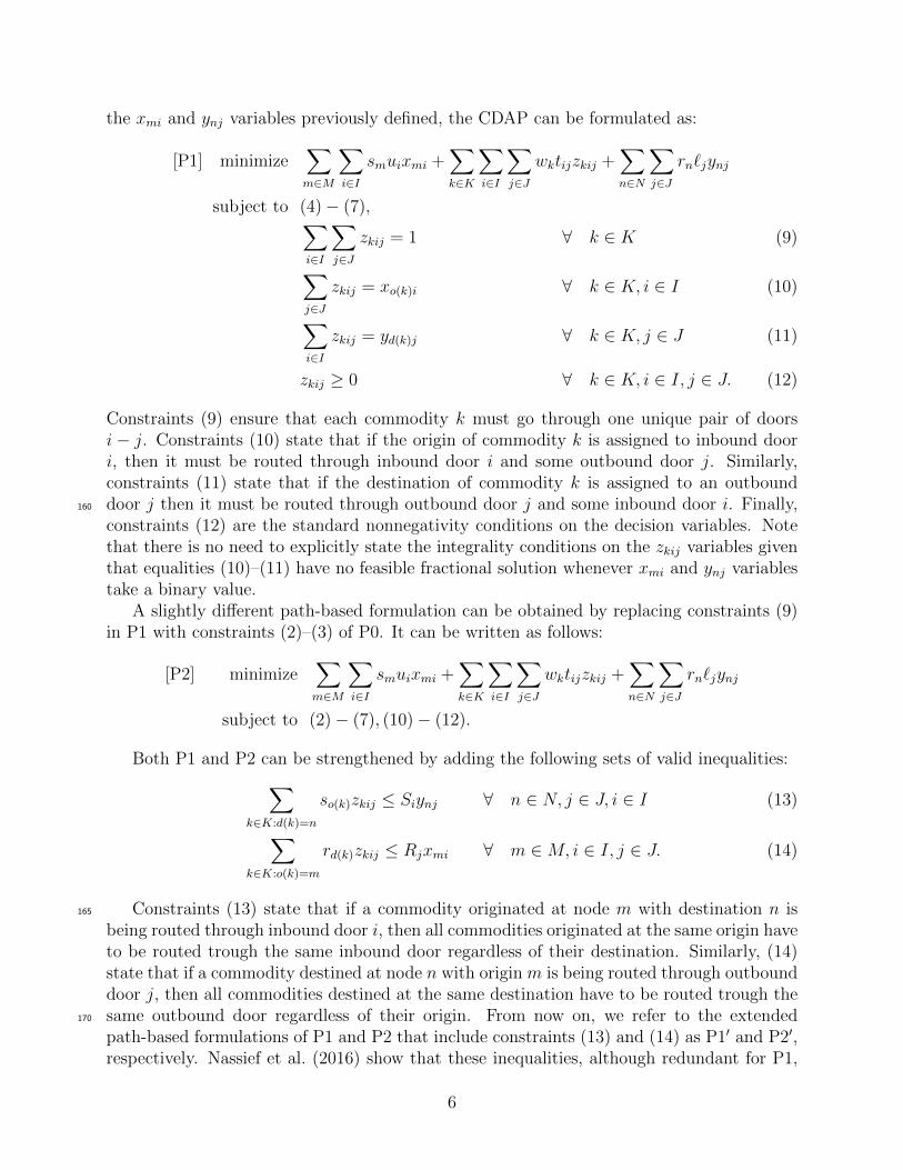
the xmi and ynj variables previously defined, the CDAP can be formulated as:

[P1] minimize∑m∈M

∑i∈I

smuixmi +∑k∈K

∑i∈I

∑j∈J

wktijzkij +∑n∈N

∑j∈J

rn`jynj

subject to (4)− (7),∑i∈I

∑j∈J

zkij = 1 ∀ k ∈ K (9)∑j∈J

zkij = xo(k)i ∀ k ∈ K, i ∈ I (10)∑i∈I

zkij = yd(k)j ∀ k ∈ K, j ∈ J (11)

zkij ≥ 0 ∀ k ∈ K, i ∈ I, j ∈ J. (12)

Constraints (9) ensure that each commodity k must go through one unique pair of doorsi − j. Constraints (10) state that if the origin of commodity k is assigned to inbound doori, then it must be routed through inbound door i and some outbound door j. Similarly,constraints (11) state that if the destination of commodity k is assigned to an outbounddoor j then it must be routed through outbound door j and some inbound door i. Finally,160

constraints (12) are the standard nonnegativity conditions on the decision variables. Notethat there is no need to explicitly state the integrality conditions on the zkij variables giventhat equalities (10)–(11) have no feasible fractional solution whenever xmi and ynj variablestake a binary value.

A slightly different path-based formulation can be obtained by replacing constraints (9)in P1 with constraints (2)–(3) of P0. It can be written as follows:

[P2] minimize∑m∈M

∑i∈I

smuixmi +∑k∈K

∑i∈I

∑j∈J

wktijzkij +∑n∈N

∑j∈J

rn`jynj

subject to (2)− (7), (10)− (12).

Both P1 and P2 can be strengthened by adding the following sets of valid inequalities:∑k∈K:d(k)=n

so(k)zkij ≤ Siynj ∀ n ∈ N, j ∈ J, i ∈ I (13)

∑k∈K:o(k)=m

rd(k)zkij ≤ Rjxmi ∀ m ∈M, i ∈ I, j ∈ J. (14)

Constraints (13) state that if a commodity originated at node m with destination n is165

being routed through inbound door i, then all commodities originated at the same origin haveto be routed trough the same inbound door regardless of their destination. Similarly, (14)state that if a commodity destined at node n with origin m is being routed through outbounddoor j, then all commodities destined at the same destination have to be routed trough thesame outbound door regardless of their origin. From now on, we refer to the extended170

path-based formulations of P1 and P2 that include constraints (13) and (14) as P1′ and P2′,respectively. Nassief et al. (2016) show that these inequalities, although redundant for P1,

6

play an important role in improving its linear programming (LP) relaxation bound. Finally,we note that these inequalities can also be derived by using the reformulation linearizationtechnique of Sherali and Adams (2013).175

3.2. A flow-based formulation

The CDAP can be seen as a particular case of a multi-commodity network design problem(MCNDP), where the assignment decisions here correspond to the link activation decisionsin the MCNDP. The interested reader may refer to (e.g., Crainic et al., 2001) for information.Thus, it can be modeled using the so-called flow-based variables to compute the amount offlow originated at m routed between i − j doors. For each m ∈ M , i ∈ I, j ∈ J we definecontinuous variables fmij equal to the amount of flow originated at m routed from inbounddoor i to outbound door j. Using these variables, we introduce a flow-based formulation ofthe CDAP problem as follows:

[F1] minimize∑m∈M

∑i∈I

smuixmi +∑m∈M

∑i∈I

∑j∈J

tijfmij +∑n∈N

∑j∈J

rn`jynj

subject to (2)− (7) (15)∑j∈J

fmij = smxmi ∀ m ∈M, i ∈ I (16)∑i∈I

fmij =∑n∈N

wmnynj ∀ m ∈M, j ∈ J (17)

fmij ≥ 0 ∀ m ∈M, i ∈ I, j ∈ J. (18)

Constraints (16) and (17) are the flow conservation constraints for inbound and outbounddoors. In particular, constraints (16) ensure that if an origin m is assigned to inbound doori, then the total flow coming from origin m must be exactly the same as the total flowsplit through all outbound doors j. Similarly, (17) guarantee that for a given origin m and180

outbound door j, the total outgoing flow to destinations that are assigned to outbound doorj is equal to the total incoming flow at outbound door j. Finally, constraints (18) are thestandard nonnegativity conditions. A similar flow-based formulation can be obtained byredefining the fmij variables as fnij for each n ∈ N , i ∈ I and j ∈ J .

3.3. A configuration-based formulation185

We next present a formulation for the CDAP which uses configuration-based variables tocharacterize the feasible subsets of origins and destinations that can be assigned to inboundand outbound doors, respectively.

We denote by Ωci the set of configurations for inbound door i that satisfy the capacity

constraints:Ωci = M ′ ⊆M :

∑m∈M ′

sm ≤ Si.

We define a binary parameter, acm to be equal to 1 if an origin m is assigned to inbound doori in configuration c ∈ Ωc

i . Similarly, we denote by Ωhj the set of configurations for outbound

door j that satisfy the capacity constraints:

Ωhj = N ′ ⊆ N :

∑n∈N ′

rn ≤ Rj.

7

We also define a binary parameter, bhn to be equal to 1 if a destination n is assigned tooutbound door j in configuration h ∈ Ωh

j . For each inbound door i ∈ I and configuration190

c ∈ Ωci , we define binary variables xc equal to 1 if and only if configuration c is selected

for inbound door i. For each outbound door j ∈ J and configuration h ∈ Hj, we definebinary variables yh equal to 1 if and only if configuration h is selected for outbound doorj. Using these two sets of configuration-based variables, together with the zkij variablesdefined in Section 3.1, (i.e., zkij = 1 if commodity k travels from door i to door j), the195

configuration-based formulation can be written as follows:

[DC] minimize∑c∈Ωc

i

∑m∈M

∑i∈I

smuiacmx

c +∑k∈K

∑i∈I

∑j∈J

wktijzkij +∑h∈Ωh

j

∑n∈N

∑j∈J

rn`jbhny

h

subject to (9), (12)∑j∈J

zkij =∑c∈Ωc

i

aco(k)xc ∀ k ∈ K, i ∈ I (19)

∑i∈I

zkij =∑h∈Ωh

j

bhd(k)yh ∀ k ∈ K, j ∈ J (20)

∑c∈Ωc

i

xc = 1 ∀ i ∈ I (21)

∑h∈Ωh

j

yh = 1 ∀ j ∈ J (22)

xc ∈ 0, 1 ∀ i ∈ I, c ∈ Ωci (23)

yh ∈ 0, 1 ∀ j ∈ J, h ∈ Ωhj . (24)

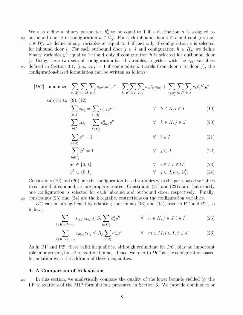
Constraints (19) and (20) link the configuration-based variables with the path-based variablesto ensure that commodities are properly routed. Constraints (21) and (22) state that exactlyone configuration is selected for each inbound and outbound door, respectively. Finally,constraints (23) and (24) are the integrality restrictions on the configuration variables.200

DC can be strengthened by adapting constraints (13) and (14), used in P1′ and P2′, asfollows: ∑

k∈K:d(k)=n

so(k)zkij ≤ Si∑h∈Ωh

j

bhnyh ∀ n ∈ N, j ∈ J, i ∈ I (25)

∑k∈K:o(k)=m

rd(k)zkij ≤ Rj

∑c∈Ωc

i

acmxc ∀ m ∈M, i ∈ I, j ∈ J. (26)

As in P1′ and P2′, these valid inequalities, although redundant for DC, play an importantrole in improving its LP relaxation bound. Hence, we refer to DC ′ as the configuration-basedformulation with the addition of these inequalities.

4. A Comparison of Relaxations

In this section, we analytically compare the quality of the lower bounds yielded by the205

LP relaxations of the MIP formulations presented in Section 3. We provide dominance or

8

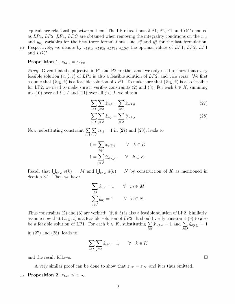
equivalence relationships between them. The LP relaxations of P1, P2, F1, and DC denotedas LP1, LP2, LF1, LDC are obtained when removing the integrality conditions on the xmiand ynj variables for the first three formulations, and xci and yhj for the last formulation.Respectively, we denote by zLP1, zLP2, zLF1, zLDC the optimal values of LP1, LP2, LF1210

and LDC.

Proposition 1. zLP1 = zLP2.

Proof. Given that the objective in P1 and P2 are the same, we only need to show that everyfeasible solution (x, y, z) of LP1 is also a feasible solution of LP2, and vice versa. We firstassume that (x, y, z) is a feasible solution of LP1. To make sure that (x, y, z) is also feasiblefor LP2, we need to make sure it verifies constraints (2) and (3). For each k ∈ K, summingup (10) over all i ∈ I and (11) over all j ∈ J , we obtain∑

i∈I

∑j∈J

zkij =∑i∈I

xo(k)i (27)∑i∈I

∑j∈J

zkij =∑j∈J

yd(k)j. (28)

Now, substituting constraint∑i∈I

∑j∈J

zkij = 1 in (27) and (28), leads to

1 =∑i∈I

xo(k)i ∀ k ∈ K

1 =∑j∈J

yd(k)j. ∀ k ∈ K.

Recall that⋃k∈K o(k) = M and

⋃k∈K d(k) = N by construction of K as mentioned in

Section 3.1. Then we have ∑i∈I

xmi = 1 ∀ m ∈M∑j∈J

ynj = 1 ∀ n ∈ N.

Thus constraints (2) and (3) are verified: (x, y, z) is also a feasible solution of LP2. Similarly,assume now that (x, y, z) is a feasible solution of LP2. It should verify constraint (9) to alsobe a feasible solution of LP1. For each k ∈ K, substituting

∑i∈Ixo(k)i = 1 and

∑j∈J

yd(k)j = 1

in (27) and (28), leads to ∑i∈I

∑j∈J

zkij = 1, ∀ k ∈ K

and the result follows.

A very similar proof can be done to show that zP1′ = zP2′ and it is thus omitted.

Proposition 2. zLF1 ≤ zLP2.215

9

Proof. We will show that every feasible solution (x, y, z) of LP2 is also a feasible solutionof LF1, which satisfies constraints (16), (17) and (18). Summing up (10) over k ∈ K suchthat o(k) = m and multiplying by wk, we obtain∑

k∈K:o(k)=m

∑j∈J

wkzkij =∑

k∈K:o(k)=m

wkxmi = smxmi (29)

for each m ∈M , i ∈ I, where the second equality follows from∑

k∈K:o(k)=mwk = sm for eachm ∈M . Let

fmij =∑

k∈K:o(k)=m

wkzkij. (30)

Summing over j in (30) and using (29) leads to:∑j∈J

fmij =∑j∈J

∑k∈K:o(k)=m

wkzkij = smxmi ∀ m ∈M, i ∈ I,

which corresponds to constraints (16).We now sum up (11) over k ∈ K such that o(k) = m. Multiplying by wk, we obtain∑

k∈K:o(k)=m

∑i∈I

wkzkij =∑

k∈K:o(k)=m

wkyd(k)j =∑n∈N

wmnynj, (31)

for each m ∈M , j ∈ J . Summing over i in (30) and using (31) leads to:∑i∈I

fmij =∑n∈N

wmnynj ∀ m ∈M, j ∈ J,

which corresponds to constraints (17) and the result follows. Note that constraints (12) and(30) combined ensure that constraints (18) are satisfied.

Proposition 3. zLP1 ≤ zLDC.

Proof. In P1, we relax constraints (10) and (11) in a Lagrangean fashion weighting their220

violations with a multiplier vector (µ, ν) of appropriate dimension as seen in Nassief et al.(2016). In this paper, however, the only difference is in the additional linear terms of unload-ing/loading times in the objective function. Therefore, we obtain the following Lagrangeanfunction:

L(µ, ν) = min(z,x,y)

∑m∈M

∑i∈I

smuixmi +∑k∈K

∑i∈I

∑j∈J

wktijzkij +∑n∈N

∑j∈J

rn`jynj

+∑k∈K

∑i∈I

µki

(∑j∈J

zkij − xo(k)i

)

+∑k∈K

∑j∈J

νkj

(∑i∈I

zkij − yd(k)j

): (4)− (9), (12)

,

10

and its associated Lagrangean dual problem

zLD = maxµ,ν

L(µ, ν).

It is then equivalent to the following linear program (Geoffrion, 1974):

[PR] minimize∑m∈M

∑i∈I

smuixmi +∑k∈K

∑i∈I

∑j∈J

wktijzkij +∑n∈N

∑j∈J

rn`jynj

subject to:∑j∈J

zkij = xo(k)i k ∈ K, i ∈ I (10)∑i∈I

zkij = yd(k)j k ∈ K, j ∈ J (11)

(x, y, z) ∈ Co

(x, y, z) ∈ B|M ||I| ×B|N ||J | ×R|K||I||J |+ :∑i∈I

∑j∈J

zkij = 1, k ∈ K,

∑m∈M

smxmi ≤ Si, i ∈ I,∑n∈N

rnynj ≤ Rj, j ∈ J

, (32)

where Co X denotes the convex hull of X.225

Taking into account that the convex hull in (32) is the intersection of several independentpolytopes Z ∪X ∪ Y , where Z =

⋃k∈K Zk, X =

⋃i∈I Xi, Y =

⋃j∈J Yj, and

Zk = Co

zk ∈ R|I||J |+ :

∑i∈I

∑j∈J

zkij = 1

,

Xi = Co

xi ∈ B|M | :

∑m∈M

smxmi ≤ Si

,

Yj = Co

yj ∈ B|N | :

∑n∈N

rnynj ≤ Rj

,

Note that Zk =

zk ∈ R|I||J |+ :

∑i∈I

∑j∈J

zkij = 1

because of total unimodularity. PR is then

equivalent to the linear program:

[PR′] minimize∑m∈M

∑i∈I

smuixmi +∑k∈K

∑i∈I

∑j∈J

wktijzkij +∑n∈N

∑j∈J

rn`jynj

11

subject to:∑i∈I

∑j∈J

zkij = 1 ∀ k ∈ K (9)∑j∈J

zkij = xo(k)i ∀ k ∈ K, i ∈ I (10)∑i∈I

zkij = yd(k)j ∀ k ∈ K, j ∈ J (11)

xi ∈ Co

xi ∈ B|M | :

∑m∈M

smxmi ≤ Si

∀ i ∈ I

yj ∈ Co

yj ∈ B|N | :

∑n∈N

rnynj ≤ Rj

∀ j ∈ J

zkij ≥ 0 ∀ k ∈ K, i ∈ I, j ∈ J.(12)

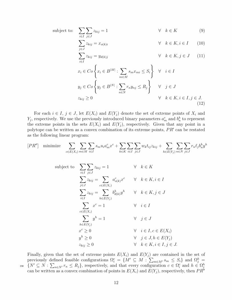
For each i ∈ I, j ∈ J , let E(Xi) and E(Yj) denote the set of extreme points of Xi andYj, respectively. We use the previously introduced binary parameters acm and bhn to representthe extreme points in the sets E(Xi) and E(Yj), respectively. Given that any point in apolytope can be written as a convex combination of its extreme points, PR′ can be restatedas the following linear program:

[PR′′] minimize∑

c∈E(Xi)

∑m∈M

∑i∈I

smuiacmx

c +∑k∈K

∑i∈I

∑j∈J

wktijzkij +∑

h∈E(Yj)

∑n∈N

∑j∈J

rn`jbhny

h

subject to∑i∈I

∑j∈J

zkij = 1 ∀ k ∈ K∑j∈J

zkij =∑

c∈E(Xi)

aco(k)xc ∀ k ∈ K, i ∈ I

∑i∈I

zkij =∑

h∈E(Yj)

bhd(k)yh ∀ k ∈ K, j ∈ J

∑c∈E(Xi)

xc = 1 ∀ i ∈ I

∑h∈E(Yj)

yh = 1 ∀ j ∈ J

xc ≥ 0 ∀ i ∈ I, c ∈ E(Xi)

yh ≥ 0 ∀ j ∈ J, h ∈ E(Yj)

zkij ≥ 0 ∀ k ∈ K, i ∈ I, j ∈ J.

Finally, given that the set of extreme points E(Xi) and E(Yj) are contained in the set ofpreviously defined feasible configurations Ωc

i = M ′ ⊆ M :∑

m∈M ′ sm ≤ Si and Ωhj =

N ′ ⊆ N :∑

n∈N ′ rn ≤ Rj, respectively, and that every configuration c ∈ Ωci and h ∈ Ωh

j230

can be written as a convex combination of points in E(Xi) and E(Yj), respectively, then PR′′

12

is equivalent to the LP relaxation of DC and thus, we have zP1 ≤ zLD = zLDC , and the resultfollows. As will be shown in Section 6, zP1 is often smaller than zLDC . This is explained bythe fact that the Lagrangean dual problem does not have the integrality property.

4.1. A Combinatorial Relaxation235

We now present a simple combinatorial bound for the CDAP which can be obtained byusing the information on the minimum handling cost of unloading, loading and transferringcommodities between door pairs for every k ∈ K. In particular, when relaxing the linkingconstraints (10), (11) and the capacity constraints (5), (4) from P2 and adding constraints(9), we obtain the following combinatorial relaxation:

(COMB) zCOMB = minimize∑m∈M

∑i∈I

smuixmi+∑k∈K

∑i∈I

∑j∈J

wktijzkij +∑n∈N

∑j∈J

rn`jynj

subject to∑i∈I

∑j∈J

zkij = 1 ∀ k ∈ K∑i∈I

xmi = 1 ∀ m ∈M∑j∈J

ynj = 1 ∀ n ∈ N

xmi ∈ 0, 1 ∀ m ∈M, i ∈ Iynj ∈ 0, 1 ∀ n ∈ N, j ∈ Jzkij ≥ 0 ∀ k ∈ K, i ∈ I, j ∈ J.

Proposition 4. zCOMB ≤ zLF1.

Proof. COMB can be decomposed into three independent subproblems, one for each set ofx, y, and z variables, respectively. The subproblems in the space of the x and y variablescan be further decomposed into several independent semi-assignment problems which can besolved by inspection. Given that the cost tij does not depend on commodity k, the optimalsolution of the third subproblem is given by the path having the shortest cost. Therefore,we have

zCOMB =∑m∈M

smumini +

∑k∈K

wktminij +

∑n∈N

rn`minj ,

where umini = min ui : i ∈ I, tminij = min tij : i ∈ I, j ∈ J, and `minj = min `j : j ∈ J.Consider now a relaxation of F1, denoted as RF1, where all constraints but (2), (3), and(16) are relaxed. Summing up (16) over i ∈ I, we obtain∑

i∈I

∑j∈J

fmij = sm∑i∈I

xmi = sm,

where the last equality follows from (2). Thus, an optimal solution to RF1 is given byrouting the flow originated at each origin m ∈M through the door pair having the smallestunloading and transfer cost, i.e.,

zRF1 =∑m∈M

sm mini∈I,j∈J

ui + tij+∑n∈N

rn`minj .

13

Therefore, we have zCOMB ≤ zRF1 ≤ zLF1, and the result follows.

The following corollary summarizes the results from this section.

Corollary 1. zCOMB ≤ zLF1 ≤ zLP1 = zLP2 ≤ zLDC ≤ zLDC′.

This means that in terms of the LP relaxation bounds, the best theoretical bound is240

obtained with (DC ′), whereas the flow-based formulation (F1), has the weakest lower bound.In Section 6, we present the results of computational experiments to compare the quality ofthe LP bounds of all formulations along with the combinatorial and Lagrangean bounds.

5. A Column Generation Algorithm

Column generation (CG) is a decomposition method used to solve linear programs with245

an enormous number of variables. The main idea of the method is to divide the originallinear program, denoted as the master problem (MP), into two interrelated subproblems: arestricted master problem (RMP) and a set of pricing problems (PPs). The RMP containsonly a small subset of the columns (or variables) of the original MP. At every iteration,the RMP is solved to optimality and additional columns are added on the fly. The PPs250

are solved to determine whether the current solution of the RMP is optimal for the MP orto identify additional columns with negative reduced costs to be added to the RMP. Thisprocess is repeated as long as new columns with negative reduced costs can be identified; itterminates when an ε-optimal solution for the MP has been identified.

We next present a CG algorithm to solve the LP relaxation of the configuration-based255

formulation DC ′. In addition, initial columns and termination criterion are explained briefly.

5.1. The restricted master problem

Let Ωci(t) denote the subset of configurations for inbound door i at iteration t, Ωh

j(t) denotethe subset of feasible configurations for outbound door j at iteration t, and Dk(t) the subsetof available door pairs for commodity k at iteration t. The RMP at iteration t can be statedas follows:

[RMP(t)] minimize∑c∈Ωc

i(t)

∑m∈M

∑i∈I

smuiacmx

c +∑k∈K

∑(i,j)∈Dk(t)

wkdijzkij +∑

h∈Ωhj(t)

∑n∈N

∑j∈J

rn`ibhny

h

14

subject to:∑

(i,j)∈Dk(t)

zkij = 1 ∀ k ∈ K (33)

∑(i,j)∈Dk(t)

zkij =∑c∈Ωc

i(t)

aco(k)xc ∀ k ∈ K, i ∈ I (34)

∑(i,j)∈Dk(t)

zkij =∑

h∈Ωhj(t)

bhd(k)yh ∀ k ∈ K, j ∈ J (35)

∑k∈K:d(k)=n

∑(i,j)∈Dk(t)

so(k)zkij ≤ Si∑

h∈Ωhj(t)

bhnyh ∀ n ∈ N, j ∈ J, i ∈ I (36)

∑k∈K:o(k)=m

∑(i,j)∈Dk(t)

rd(k)zkij ≤ Rj

∑c∈Ωc

i(t)

acmxc ∀ m ∈M, i ∈ I, j ∈ J (37)

∑c∈Ωc

i(t)

xc = 1 ∀ i ∈ I (38)

∑h∈Ωh

j(t)

yh = 1 ∀ j ∈ J (39)

xc ≥ 0 ∀ c ∈ Ωci(t) (40)

yh ≥ 0 ∀ h ∈ Ωhj(t) (41)

zkij ≥ 0 ∀ k ∈ K, (i, j) ∈ Dk(t). (42)

Note that, although there is a polynomial number of routing variables zkij, we do notadd all of them as very few of them will be used in an optimal solution of the LP relaxationof DC ′.260

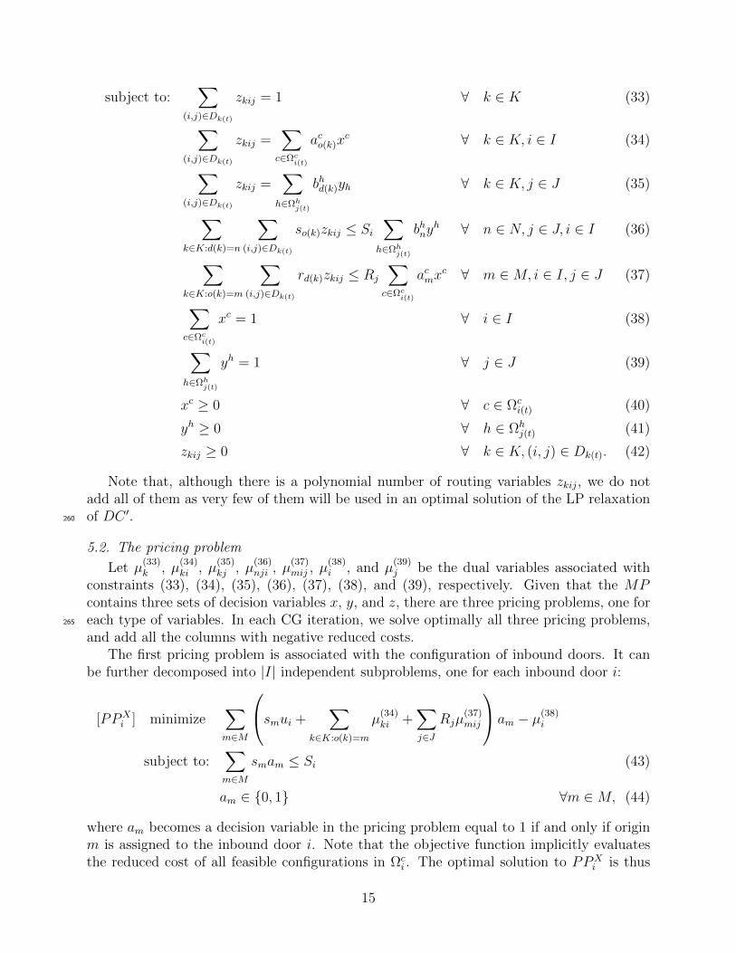
5.2. The pricing problem

Let µ(33)k , µ

(34)ki , µ

(35)kj , µ

(36)nji , µ

(37)mij , µ

(38)i , and µ

(39)j be the dual variables associated with

constraints (33), (34), (35), (36), (37), (38), and (39), respectively. Given that the MPcontains three sets of decision variables x, y, and z, there are three pricing problems, one foreach type of variables. In each CG iteration, we solve optimally all three pricing problems,265

and add all the columns with negative reduced costs.The first pricing problem is associated with the configuration of inbound doors. It can

be further decomposed into |I| independent subproblems, one for each inbound door i:

[PPXi ] minimize

∑m∈M

smui +∑

k∈K:o(k)=m

µ(34)ki +

∑j∈J

Rjµ(37)mij

am − µ(38)i

subject to:∑m∈M

smam ≤ Si (43)

am ∈ 0, 1 ∀m ∈M, (44)

where am becomes a decision variable in the pricing problem equal to 1 if and only if originm is assigned to the inbound door i. Note that the objective function implicitly evaluatesthe reduced cost of all feasible configurations in Ωc

i . The optimal solution to PPXi is thus

15

the configuration for an inbound door i having the smallest reduced cost. PPXi is a 0-1270

knapsack problem which is known to be NP-hard. However, it can be efficiently solved usingthe 0-1 knapsack algorithm given in Martello et al. (2000).

The second pricing problem is associated with the configuration of outbound doors. Itcan also be further decomposed into |J | independent subproblems, one for each outbounddoor j:

[PP Yj ] minimize

∑n∈N

rn`i +∑

k∈K:d(k)=n

µ(35)kj +

∑i∈I

Siµ(36)nji

bn − µ(39)j

subject to:∑n∈N

rnbn ≤ Rj (45)

bn ∈ 0, 1 ∀ n ∈ N, (46)

where bn becomes a decision variable in the pricing problem equal to 1 if and only if destina-tion n is assigned to outbound door j. Similarly to PPX

i , the objective function implicitlyevaluates the reduced cost of all feasible configurations in Ωh

j . The optimal solution to PP Yj275

is thus the configuration for an outbound door j having the smallest reduced cost. PP Yj also

corresponds to a 0-1 knapsack problem and can be solved in the same way as PPXi .

Finally, the third pricing problem is associated with the routing variables zkij. It can alsobe decomposed into |K| independent subproblems which in turn, can be solved by inspection.In particular, for each commodity k, we simply identify the door pair (i, j) ∈ I × J with thesmallest reduced cost:

[PPZk ] (ik, jk) ∈ arg min(i,j)∈I×J

∑i∈I

∑j∈J

wkdij−µ(34)ki −µ

(35)kj −rd(k)µ

(37)o(k)ij−so(k)µ

(36)d(k)ji−µ

(33)k

This leads to a O(|K||I||J |) complexity for solving all PPZk pricing problems.

5.3. Initial columns

Initial columns are generated by solving two independent Generalized Assignment Prob-280

lems (GAPs). Each GAP provides feasible assignments on an inbound (outbound) side of thecross-dock. Whenever the assignments, ami and bnj are generated, we use that informationto calculate the path based variables as zkij = ao(k)ibd(k)j. Moreover, the algorithm startswith a few zkij variables that satisfy: |i − j| ≤ 1. The rest of these variables is generatedusing PPZ

k .285

5.4. Termination criterion

A valid lower bound v(LB) on the master problem MP can be obtained as seen in Amoret al. (2009), and then be used in a termination criterion. Such a valid lower bound iscalculated iteratively via solving relaxations of the RMP . At each CG iteration, wheneverwe price out new variables or columns from the pricing problems, PPX

i , PP Yj and PPZ

k ,their incorporation will decrease the current optimal value associated with the RMP , i.e.,v(RMP t). For simplicity, we restate PPX

i , PP Yj and PPZ

k as PPi, PPj and PPk, respec-tively. The valid lower bound for a given iteration t can be stated as follows:

v(LBt) = v(RMP t) +∑i∈I

v(PP ti )− µ

(38)i +

∑j∈J

v(PP tj )− µ

(39)j +

∑k∈K

v(PP tk)− µ

(33)k

16

The dual variables µ(38)i , µ

(39)j and µ

(33)k are associated with the convexity constraints (38),

(39) and (33), respectively. Hence, they are singled out. Finally, we use this computation toterminate CG whenever: v(LBt)− v(RMP t) ≤ 10−6

5.5. The Lagrangean Dual Problem290

The Lagrangean dual problem reported in this paper differs than the one reported inNassief et al. (2016) only in the additional linear terms of the objective function of P1′.Hence, it modifies slightly the objective terms in the subproblems of the Lagrangean dual.Both Lagrangean dual problems consist of the same three independent subproblems. Twoof which are 0-1 knapsack subproblems, and one of which is a semi-assignment subproblem.295

The knapsack subproblems are solved efficiently using the 0-1 knapsack algorithm given inMartello et al. (2000), while the semi-assignment subproblems are solved by inspection.

6. Computational Experiments

In this section, we present the results of computational experiments performed to assessthe behavior of the MIP formulations, combinatorial, linear and Lagrangean relaxations300

for the CDAP. All algorithms were coded in C and run on an Intel Xeon E3 1240 V2processor with 3.40 GHz and 24GB of RAM memory under a Windows environment. TheMIP formulations and CG algorithm were implemented using the callable library of CPLEX12.6.2. We first explain the data set generation, then the tuning of the parameters andfinally, the computational comparisons and analysis.305

6.1. Data Set Generation

We use the benchmark data set introduced by Guignard et al. (2012) for the CDAP withtransfer times only, and then, we extend it to include unloading/loading times.

Guignard et al. (2012) generate the flow matrix with integer numbers between [10, 50]until 25% of the matrix is full. The distance (or travel time) matrix is generated within310

the interval [τ, τ + I − 1], where τ = 8 indicates the distance between two doors facing eachother, and then an increment of 1 unit is added for the next closest door. All instances aregenerated with |I| = |J | for a rectangular shaped cross-dock. Capacities are identical andcalculated by dividing the total flow coming from all origins by the total number of inbounddoors, and then adding some capacity slackness. A total of 50 instances are considered from315

the possible combinations of these parameters and are denoted as 00x00S00. The first posi-tion refers to the number of origins/destinations, taken in 8, 9, 10, 11, 12, 15, 20. The secondposition refers to the number of inbound/outbound doors, taken in 4, 5, 6, 7, 10. The thirdposition refers to the capacity slackness which are drawn from 5%, 10%, 15%, 20%, 30%.

We generate the additional parameters of unloading/loading times as follows. Using320

a private communication with a large cross-dock company1, and based on their data, wefind out that it is generally assumed that the total handling time of shipments inside thecross-dock is divided approximately into 22% for unloading, 43% for traveling, and 35% forloading. These percentages are approximated based on the company’s standard operating

1The company does not want to be identified

17

procedures of unloading, transferring and loading shipments inside the cross-dock facility for325

an average truck. We observe that traveling time takes the largest portion of handling timeinside the cross-dock, while loading is 1.5 to 2 times longer than unloading as mentioned inZhang et al. (2010). As mentioned in Bartholdi III and Hackman (2011), loading is moredifficult than unloading as the loader employee has to make sure the truck is fully packed.Therefore, using a uniform distribution, we generate the unloading and loading times with330

the above distribution with respect to the previously generated traveling time matrix. Thatis for i ∈ I, ui = 0.5 ∗ random[τ, τ + I − 3] where about 50% ≈ 22

43100, and for j ∈ J ,

`j = 0.8 ∗ random[τ, τ + I − 3] where 80% ≈ 3543

100. The expression τ + I − 3 was obtainedafter some fine tuning so that the 20%, 34%, 35% percentages are observed at optimalsolution values.335

6.2. Tuning and Termination Criteria of the Algorithms

The following parameters were fine tuned with preliminary experiments so as to offerthe best compromise between the quality of the solutions and computational times. For theMIP formulations, we use the deterministic parallel branch-and-cut algorithm of CPLEXwith 6 threads and the central processing unit (CPU) time limit was set to 7,200 seconds340

(i.e., 2 hours). The remaining CPLEX parameters were kept to their default value. For thestandard CDAP, the sub-gradient method was implemented as explained in Nassief et al.(2016), reporting only lower bounds and CPU times. For the CDAP with unloading/loadingtimes, the LR was adapted to incorporate the additional linear terms and the subgradientmethod was also used to solve the associated Lagrangean dual problem. The maximum345

number of iterations was set to 300,000, the step length parameter ε was multiplied by 0.9every 2,000 consecutive iterations without improvement of the lower bound and reset to 2whenever ε < 10−7.

6.3. Comparisons of formulations and relaxations

In the following experiments, we compare the results obtained with the MIP formulations,350

the combinatorial relaxation, and lower bounds obtained by CG and LR. The detailed andsummarized results of these comparisons are given in Table 1 for the CDAP with unload-ing/loading times, and in Table 2 for the standard CDAP. In all four tables, the first columngives the name of the instance. The last rows report its %LP deviation with the respectto the optimal solution, the remaining optimality %gap when terminating, the number of355

explored branch and bound (B&B) nodes, and the CPU time in seconds. The LP deviationis calculated as %LP = 100(OPT−LP )/(OPT ), where OPT is the optimal value and LP isthe optimal solution for the LP relaxation of each formulation. For P1 and P2, we show theLP deviation with and without the valid inequalities (13) and (14), that is %LP ′ and %LP ,respectively. The combinatorial bounds are obtained in less than a second for all instances,360

and so we report only on the quality of their bounds. For the LR, we report the deviation ofthe best obtained lower bound and CPU time after termination. For the DC ′ formulation,we report its %LP using CG algorithm and the CPU time. Finally, we use P1 and P2instead of P1′ and P2′ to obtain optimal solutions in CPLEX as the former outperform thelatter with respect to the required CPU time and remaining %gap for unsolved instances.365

This is partially attributed to a substantial increase in the required CPU time to solve theLP relaxations of P1′ and P2′ due to the large number of dense constraints added.

18

Table 1: Computational Comparisons - CDAP

Instances Path-based (P1) Path-based (P2) Flow-based (F1) COMB LR’ DC’

%LP %LP’ %gap B&B CPU %LP %LP’ %gap B&B CPU %LP %gap B&B CPU %LB %LB CPU %LB CPU

8x4S5 3.12 1.56 0.00 42 0.20 3.12 1.56 0.00 0 0.07 3.12 0.00 0 0.07 5.20 1.50 28.58 1.14 0.15

8x4S10 2.95 1.53 0.00 100 0.10 2.95 1.53 0.00 89 0.13 2.95 0.00 172 0.14 4.08 3.22 24.76 1.32 0.14

8x4S15 3.11 1.73 0.00 63 0.11 3.11 1.73 0.00 0 0.09 3.11 0.00 0 0.11 5.92 4.86 27.34 1.25 0.14

8x4S20 2.77 1.27 0.00 0 0.07 2.77 1.27 0.00 0 0.12 2.77 0.00 0 0.12 4.68 7.15 26.05 0.87 0.09

8x4S30 2.39 1.17 0.00 127 0.21 2.39 1.17 0.00 74 0.11 2.39 0.00 0 0.11 6.04 11.30 26.46 1.05 0.11

9x4S5 3.36 1.65 0.00 187 0.17 3.36 1.65 0.00 116 0.12 3.36 0.00 0 0.09 8.14 2.32 28.39 1.45 0.16

9x4S10 3.35 1.63 0.00 126 0.13 3.35 1.63 0.00 156 0.09 3.35 0.00 0 0.23 7.40 4.36 27.91 1.52 0.12

9x4S15 3.33 1.62 0.00 107 0.09 3.33 1.62 0.00 64 0.08 3.33 0.00 66 0.10 5.71 6.90 28.29 1.36 0.11

9x4S20 3.13 1.58 0.00 57 0.09 3.13 1.58 0.00 0 0.04 3.13 0.00 128 0.11 3.53 9.78 29.58 1.27 0.11

9x4S30 3.34 1.52 0.00 100 0.11 3.34 1.52 0.00 92 0.08 3.34 0.00 114 0.10 4.85 14.30 30.83 1.48 0.12

10x4S5 3.92 2.89 0.00 399 0.22 3.92 2.89 0.00 417 0.26 3.92 0.00 1,411 0.26 5.14 4.15 33.10 2.82 0.18

10x4S10 2.52 1.59 0.00 219 0.14 2.52 1.59 0.00 160 0.12 2.52 0.00 350 0.16 5.77 4.28 34.25 1.58 0.17

10x4S15 2.53 1.60 0.00 133 0.15 2.53 1.60 0.00 249 0.20 2.53 0.00 327 0.13 6.49 7.28 37.56 1.54 0.13

10x4S20 2.54 1.64 0.00 276 0.13 2.54 1.64 0.00 185 0.13 2.54 0.00 405 0.16 5.66 9.75 33.89 1.60 0.16

10x4S30 1.50 0.91 0.00 0 0.06 1.50 0.91 0.00 52 0.08 1.50 0.00 161 0.18 5.12 13.13 36.54 0.88 0.15

10x5S5 4.24 2.87 0.00 750 0.45 4.24 2.87 0.00 519 0.39 4.24 0.00 1,304 0.78 11.13 3.14 39.64 2.60 0.19

10x5S10 3.54 2.29 0.00 638 0.31 3.54 2.29 0.00 619 0.28 3.54 0.00 1,414 0.54 8.84 4.89 40.67 2.06 0.18

10x5S15 3.04 1.92 0.00 502 0.36 3.04 1.92 0.00 508 0.28 3.04 0.00 873 0.47 10.56 5.07 42.11 1.77 0.21

10x5S20 2.97 1.88 0.00 194 0.29 2.97 1.88 0.00 183 0.21 2.97 0.00 648 0.39 9.58 7.20 42.83 1.43 0.22

10x5S30 3.15 2.21 0.00 460 0.30 3.15 2.21 0.00 530 0.27 3.15 0.00 1,531 0.53 8.94 10.90 42.16 1.95 0.23

11x5S5 4.88 3.37 0.00 1,911 0.88 4.88 3.37 0.00 2,162 0.75 4.88 0.00 1,701 0.95 8.60 4.02 46.88 3.11 0.35

11x5S10 3.59 2.07 0.00 552 0.37 3.59 2.07 0.00 822 0.41 3.59 0.00 3,458 1.22 10.45 5.00 47.92 1.91 0.32

11x5S15 3.36 2.13 0.00 436 0.36 3.36 2.13 0.00 760 0.42 3.36 0.00 3,308 1.26 9.07 7.30 47.11 1.99 0.23

11x5S20 3.21 2.05 0.00 394 0.28 3.21 2.05 0.00 387 0.25 3.21 0.00 3,360 1.41 10.90 8.11 49.84 1.83 0.28

11x5S30 2.87 1.83 0.00 459 0.33 2.87 1.83 0.00 302 0.44 2.87 0.00 1,404 0.57 6.37 12.33 59.85 1.77 0.28

12x5S5 3.81 2.53 0.00 876 0.81 3.81 2.53 0.00 711 0.58 3.81 0.00 1,084 0.80 7.97 3.26 65.46 2.12 0.40

12x5S10 3.15 2.02 0.00 878 0.62 3.15 2.02 0.00 956 0.61 3.15 0.00 3,027 1.31 7.26 5.44 65.96 1.96 0.34

12x5S15 3.14 2.10 0.00 697 0.57 3.14 2.10 0.00 770 0.63 3.14 0.00 1,754 0.87 7.46 6.74 66.51 1.98 0.33

12x5S20 3.20 2.28 0.00 1,301 0.78 3.20 2.28 0.00 1,369 0.65 3.20 0.00 5,585 2.04 7.46 8.33 70.18 2.14 0.33

12x5S30 3.18 2.36 0.00 4,874 2.52 3.18 2.36 0.00 2,989 1.34 3.18 0.00 3,076 1.33 6.67 12.56 75.20 2.28 0.36

12x6S5 5.92 4.50 0.00 5,298 4.19 5.92 4.50 0.00 3,863 2.86 5.92 0.00 2,525 2.09 12.09 4.54 72.47 4.03 0.97

12x6S10 4.36 2.82 0.00 1,704 1.55 4.36 2.82 0.00 2,865 1.75 4.36 0.00 3,227 2.11 10.15 4.97 75.19 2.48 0.64

12x6S15 4.46 3.02 0.00 1,845 1.51 4.46 3.02 0.00 1,883 1.33 4.46 0.00 2,844 2.25 8.49 7.14 74.56 2.63 0.61

12x6S20 3.93 2.58 0.00 3,643 2.36 3.93 2.58 0.00 3,993 2.21 3.93 0.00 4,441 3.02 12.66 8.17 71.36 2.36 0.50

12x6S30 3.83 2.70 0.00 5,288 2.59 3.83 2.70 0.00 2,902 1.62 3.83 0.00 7,012 3.51 8.73 11.75 70.89 2.48 0.54

15x6S5 4.18 2.57 0.00 24,105 29.36 4.18 2.57 0.00 18,627 18.69 4.18 0.00 57,844 52.27 15.17 4.24 99.75 2.53 1.79

15x6S10 4.10 2.53 0.00 9,397 10.30 4.10 2.53 0.00 9,903 8.98 4.10 0.00 94,988 61.39 10.14 6.51 98.04 2.48 1.70

15x6S15 3.86 2.52 0.00 19,195 20.59 3.86 2.52 0.00 18,192 16.48 3.86 0.00 135,875 81.87 12.12 7.61 100.94 2.48 1.51

15x6S20 3.92 2.66 0.00 38,414 33.57 3.92 2.66 0.00 22,273 16.87 3.92 0.00 134,754 75.27 8.31 9.72 101.89 2.63 1.52

15x6S30 3.45 2.21 0.00 13,203 8.61 3.45 2.21 0.00 10,972 6.43 3.45 0.00 99,867 64.19 12.16 12.91 105.19 2.20 1.44

15x7S5 5.77 3.58 0.00 29,282 67.59 5.77 3.58 0.00 47,041 69.74 5.77 0.00 274,350 249.63 19.44 4.34 110.26 3.40 2.76

15x7S10 5.51 3.33 0.00 31,911 52.83 5.51 3.33 0.00 19,626 29.84 5.51 0.00 481,906 387.24 17.41 5.29 115.07 3.03 3.17

15x7S15 5.96 3.56 0.00 16,870 27.98 5.96 3.56 0.00 18,970 24.99 5.96 0.00 275,122 244.73 13.88 7.19 114.69 3.26 3.14

15x7S20 5.23 3.30 0.00 35,980 59.75 5.23 3.30 0.00 40,073 58.00 5.23 0.00 361,863 300.70 10.42 9.09 115.56 3.06 2.65

15x7S30 4.21 2.62 0.00 61,949 72.24 4.21 2.62 0.00 63,788 60.13 4.21 0.00 454,743 337.91 12.11 10.25 122.10 2.51 2.14

20x10S5 7.96 5.41 2.19 329,564 time 7.96 5.41 2.56 457,147 time 7.96 2.57 982,088 time 19.37 6.19 288.61 4.99 39.59

20x10S10 6.81 4.63 2.15 411,539 time 6.81 4.63 1.51 438,959 time 6.81 2.14 1,054,134 time 25.31 6.00 285.62 3.98 41.84

20x10S15 6.90 4.77 3.29 455,900 time 6.90 4.77 3.56 521,212 time 6.90 3.74 1,184,303 time 22.13 6.72 293.04 4.43 38.33

20x10S20 7.04 5.00 3.65 460,859 time 7.04 5.00 2.84 473,477 time 7.04 3.67 1,276,100 time 19.01 8.28 293.18 4.64 35.50

20x10S30 7.47 5.05 2.83 474,231 time 7.47 5.05 3.15 547,790 time 7.47 3.45 1,416,406 time 19.90 9.44 303.20 4.78 34.36

Average 4.00 2.54 0.28 48,941 728.12 4.00 2.54 0.27 54,776 726.58 4.00 0.31 166,821 757.69 10.08 7.18 83.35 2.33 4.42

19

6.3.1. The CDAP with unloading/loading times

In terms of MIP formulations, the computational experiments in Table 1 show that bothpath-based formulations P1 and P2, and the flow-based formulation F1 are able to obtain370

the optimal solutions of 45 out of 50 instances within the time limit of 2 hours. For theremaining instances where the optimal solution is not found within 2 hours, the tightestremaining average %gap of 2.72 is obtained by P2 as opposed to 2.82 and 3.11 in P1 andF1, respectively. While both path-based formulations have the same theoretical bounds interms of their LP relaxations, P2, on average, slightly outperforms P1 in terms of required375

CPU time in the largest set of instances.In terms of relaxations, we demonstrate in this set of instances the dominance of this

new configuration-based formulation DC ′ over all other formulations, P2, and F1 that weintroduce in this paper, as well as the P1 of Nassief et al. (2016). We highlight that whileboth DC ′ and LR have the same theoretical bounds as shown in Section 4, the CG algorithm380

obtains strictly better lower bounds as compared to LR given the slow convergence of thesubgradient method. Moreover, as the capacities looses for each block of instances, CGmaintains its dominance by far as opposed to the subgradient method.

6.3.2. The standard CDAP

In terms of MIP formulations, the computational experiments in Table 2 show also that385

both path-based formulations P1 and P2, and the flow-based formulation F1 are able toobtain the optimal solutions of 45 out of 50 instances within the time limit of 2 hours. Forthe remaining instances where the optimal solution is not found within 2 hours, the tightestremaining average %gap of 4.68, this time, is obtained by P1 as opposed to 5.58 and 7.74 inP2 and F1, respectively. Contrary to the CDAP with unloading/loading times, formulation390

P1 seems to be slightly better than P2 in terms of the CPU time and remaining %gap.In terms of relaxations, we demonstrate in this set of instances, again, the dominance

of this new configuration-based formulation DC ′ over all other formulations. We highlightthat while both DC ′ and LR have the same theoretical bounds as shown in Section 4, CGalgorithm outperforms the LR in terms of the quality of the bounds as well as the CPU time.395

However, we observe from Table 2 that the subgradient method has a more stable convergenceregardless of the capacity slackness, as opposed to the case in Table 1. Moreover, we noticethat for the standard CDAP as seen in Table 2, all linear relaxation bounds of P1, P2, andF1 coincide with the combinatorial bounds even though theoretically they are better.

6.4. Sensitivity Analysis400

In these experiments, we would like to highlight the impact of some of the parameters onthe solutions obtained. The following analysis is divided into three parts: the τ parameterand its impact on the %LP gap, the unloading and loading times, and the capacities on thedoors.

6.4.1. The τ parameter405

We highlight how the τ parameter used in the generation of travel times (or distances)tij, has an impact on LP bounds. We note that due to the fact that τ appears in everysingle tij and that each commodity is routed exactly via one pair of doors (i, j), the constantterm τ |K| can be removed from the objective function. That is, the set of optimal solutions

20

Table 2: Computational Comparisons - standard CDAP

Instances Path-based (P1) Path-based (P2) Flow-based (F1) COMB LR’ DC’

%LP %LP’ %gap B&B CPU %LP %LP’ %gap B&B CPU %LP %gap B&B CPU %LB %LB CPU %LB CPU

8x4S5 6.76 3.26 0.00 0 0.08 6.76 3.26 0.00 0 0.07 6.76 0.00 0 0.06 6.76 3.51 4.62 2.80 0.20

8x4S10 6.67 3.39 0.00 45 0.12 6.67 3.39 0.00 0 0.10 6.67 0.00 229 0.26 6.67 3.63 5.19 3.10 0.16

8x4S15 5.63 2.53 0.00 0 0.08 5.63 2.53 0.00 0 0.13 5.63 0.00 0 0.05 5.63 2.87 5.38 2.24 0.11

8x4S20 5.15 2.24 0.00 0 0.18 5.15 2.24 0.00 19 0.08 5.15 0.00 0 0.14 5.15 2.49 5.47 1.97 0.09

8x4S30 4.72 2.16 0.00 61 0.08 4.72 2.16 0.00 48 0.06 4.72 0.00 0 0.11 4.72 3.62 7.12 2.16 0.07

9x4S5 7.66 3.71 0.00 100 0.13 7.66 3.71 0.00 0 0.08 7.66 0.00 0 0.18 7.66 4.19 6.45 3.44 0.14

9x4S10 7.35 3.69 0.00 77 0.09 7.35 3.69 0.00 94 0.12 7.35 0.00 235 0.09 7.35 4.17 6.16 3.47 0.13

9x4S15 6.56 3.16 0.00 75 0.21 6.56 3.16 0.00 0 0.13 6.56 0.00 0 0.05 6.56 3.54 14.04 3.05 0.14

9x4S20 5.95 2.75 0.00 0 0.09 5.95 2.75 0.00 58 0.09 5.95 0.00 132 0.08 5.95 3.34 14.69 2.72 0.10

9x4S30 5.42 2.63 0.00 0 0.04 5.42 2.63 0.00 75 0.09 5.42 0.00 222 0.08 5.42 4.41 11.32 2.63 0.07

10x4S5 8.56 6.31 0.00 384 0.16 8.56 6.31 0.00 304 0.16 8.56 0.00 1,176 0.30 8.56 6.69 9.90 6.27 0.15

10x4S10 5.77 3.67 0.00 253 0.18 5.77 3.67 0.00 179 0.12 5.77 0.00 0 0.09 5.77 4.62 10.16 3.67 0.12

10x4S15 5.34 3.45 0.00 164 0.12 5.34 3.45 0.00 71 0.10 5.34 0.00 856 0.21 5.34 4.56 12.17 3.45 0.10

10x4S20 4.90 3.19 0.00 230 0.10 4.90 3.19 0.00 131 0.18 4.90 0.00 763 0.17 4.90 4.49 12.61 3.19 0.11

10x4S30 3.76 2.35 0.00 0 0.06 3.76 2.35 0.00 0 0.06 3.76 0.00 417 0.11 3.76 3.66 13.40 2.35 0.08

10x5S5 9.79 6.48 0.00 521 0.29 9.79 6.48 0.00 510 0.29 9.79 0.00 1,242 0.67 9.79 7.20 9.24 6.32 0.17

10x5S10 7.84 4.78 0.00 515 0.24 7.84 4.78 0.00 387 0.25 7.84 0.00 1,377 0.49 7.84 5.71 11.96 4.66 0.14

10x5S15 6.71 3.87 0.00 346 0.26 6.71 3.87 0.00 334 0.22 6.71 0.00 1,530 0.46 6.71 5.18 12.18 3.76 0.15

10x5S20 5.90 3.31 0.00 77 0.19 5.90 3.31 0.00 164 0.18 5.90 0.00 1,382 0.52 5.90 4.56 12.86 3.18 0.13

10x5S30 5.39 3.17 0.00 350 0.20 5.39 3.17 0.00 414 0.20 5.39 0.00 1,937 0.59 5.39 4.32 12.69 3.17 0.17

11x5S5 10.80 7.33 0.00 1,440 0.68 10.80 7.33 0.00 1,657 0.54 10.80 0.00 2,613 1.15 10.80 8.36 14.91 6.96 0.22

11x5S10 7.98 4.77 0.00 840 0.35 7.98 4.77 0.00 663 0.36 7.98 0.00 4,156 1.17 7.98 6.02 16.51 4.68 0.22

11x5S15 7.52 4.59 0.00 529 0.28 7.52 4.59 0.00 493 0.23 7.52 0.00 5,388 1.60 7.52 5.97 14.09 4.55 0.20

11x5S20 6.33 3.61 0.00 226 0.23 6.33 3.61 0.00 82 0.27 6.33 0.00 3,435 1.04 6.33 5.00 17.60 3.59 0.19

11x5S30 6.09 3.76 0.00 251 0.22 6.09 3.76 0.00 334 0.23 6.09 0.00 4,462 1.40 6.09 5.32 19.48 3.76 0.21

12x5S5 8.23 5.28 0.00 601 0.60 8.23 5.28 0.00 494 0.49 8.23 0.00 2,133 0.89 8.23 6.06 12.24 5.19 0.36

12x5S10 7.14 4.45 0.00 296 0.33 7.14 4.45 0.00 395 0.34 7.14 0.00 3,425 1.20 7.14 5.58 15.62 4.41 0.30

12x5S15 6.69 4.21 0.00 379 0.42 6.69 4.21 0.00 352 0.36 6.69 0.00 2,122 0.58 6.69 5.44 15.31 4.17 0.27

12x5S20 6.69 4.46 0.00 708 0.49 6.69 4.46 0.00 834 0.47 6.69 0.00 3,451 0.97 6.69 5.77 18.90 4.42 0.28

12x5S30 6.50 4.61 0.00 1,437 0.64 6.50 4.61 0.00 1,468 0.64 6.50 0.00 6,455 2.15 6.50 6.29 17.26 4.61 0.24

12x6S5 13.03 9.53 0.00 4,663 3.47 13.03 9.53 0.00 5,553 3.41 13.03 0.00 15,850 8.26 13.03 10.16 15.63 9.34 0.62

12x6S10 9.41 6.06 0.00 1,395 1.01 9.41 6.06 0.00 1,214 0.88 9.41 0.00 9,452 5.04 9.41 6.57 17.72 5.99 0.44

12x6S15 8.59 5.42 0.00 1,461 1.18 8.59 5.42 0.00 873 0.89 8.59 0.00 6,413 3.25 8.59 6.36 19.65 5.41 0.47

12x6S20 8.15 5.19 0.00 1,522 1.28 8.15 5.19 0.00 1,073 0.85 8.15 0.00 15,478 7.06 8.15 6.33 23.16 5.18 0.38

12x6S30 7.39 4.82 0.00 2,120 1.20 7.39 4.82 0.00 986 0.60 7.39 0.00 10,558 4.39 7.39 6.51 29.26 4.81 0.43

15x6S5 9.93 6.14 0.00 7,304 7.85 9.93 6.14 0.00 8,525 7.03 9.93 0.00 116,161 83.31 9.93 7.04 30.87 6.10 1.73

15x6S10 9.12 5.65 0.00 7,375 7.30 9.12 5.65 0.00 4,628 4.41 9.12 0.00 232,918 135.83 9.12 6.66 32.87 5.64 1.49

15x6S15 8.87 5.66 0.00 11,507 11.25 8.87 5.66 0.00 5,777 5.30 8.87 0.00 175,697 103.78 8.87 6.97 35.63 5.66 1.37

15x6S20 8.57 5.61 0.00 9,956 8.81 8.57 5.61 0.00 10,384 7.54 8.57 0.00 219,771 109.26 8.57 7.19 29.57 5.61 1.40

15x6S30 7.54 4.98 0.00 5,262 4.91 7.54 4.98 0.00 9,127 5.93 7.54 0.00 154,866 73.06 7.54 6.77 31.36 4.98 1.37

15x7S5 13.70 8.51 0.00 25,022 43.08 13.70 8.51 0.00 61,186 84.45 13.70 0.00 411,518 350.38 13.70 9.51 21.54 8.30 2.49

15x7S10 12.28 7.44 0.00 23,452 34.56 12.28 7.44 0.00 24,173 28.17 12.28 0.00 1,719,101 1003.13 12.28 8.62 24.28 7.35 2.45

15x7S15 11.36 6.80 0.00 17,484 20.57 11.36 6.80 0.00 14,603 17.77 11.36 0.00 1,700,274 1003.46 11.36 8.13 25.45 6.77 2.30

15x7S20 10.49 6.19 0.00 11,166 13.35 10.49 6.19 0.00 7,781 9.00 10.49 0.00 603,824 396.60 10.49 7.81 34.73 6.17 2.00

15x7S30 9.83 6.06 0.00 11,864 15.06 9.83 6.06 0.00 16,646 16.63 9.83 0.00 597,416 369.92 9.83 7.90 42.17 6.05 1.95

20x10S5 17.98 12.16 2.82 429,752 time 17.98 12.16 6.71 522,011 time 17.98 7.39 986,768 time 17.98 12.96 63.76 11.99 37.15

20x10S10 16.02 10.52 2.69 476,365 time 16.02 10.52 2.04 494,121 time 16.02 6.56 1,185,087 time 16.02 11.43 69.21 10.31 32.29

20x10S15 15.73 10.61 7.23 440,472 time 15.73 10.61 5.65 419,329 time 15.73 7.21 1,428,785 time 15.73 11.13 79.04 10.53 33.95

20x10S20 15.18 10.41 5.61 407,833 time 15.18 10.41 7.65 446,603 time 15.18 9.30 1,409,018 time 15.18 11.76 82.69 10.36 30.97

20x10S30 13.98 9.73 5.07 504,245 time 13.98 9.73 5.87 497,148 time 13.98 8.22 1,846,914 time 13.98 11.35 98.46 9.71 29.90

Average 8.54 5.29 0.47 48,203 723.64 8.54 5.29 0.56 51,226 723.99 8.54 0.77 257,900 793.47 8.54 6.35 23.33 5.20 3.80

21

remain the same regardless of the τ value used in the experiments. As mentioned earlier,410

this data was generated on the assumption that a direct distance between two doors is τ = 8as in Guignard et al. (2012). However, changing this parameter and updating the matrixaccordingly, will provide different %LP deviations while maintaining the same difficulty forsolving CDAP. In Tables 3 and 4, we assign different values to τ in the interval [0, 1000]using P1 and P1’ for the both CDAPs.415

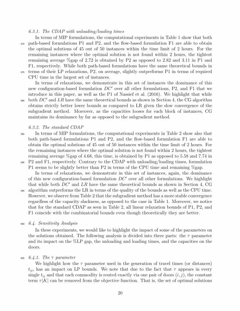
Whenever τ = 8, the %LPs clearly match the ones we reported in previous tables.However, these deviations significantly decrease(increase) as τ increases(decrease). It isthus important to keep in mind the impact of the parameter τ when computing the %LPdeviations and using them to determine how tight or good an MIP formulation might be forthe CDAPs.420

Table 3: Impact of travel times on %LP - CDAP

%LP with different τ values %LP’ with different τ values

instances 0 1 8 20 50 100 1000 0 1 8 20 50 100 1000

8x4S5 60.05 18.32 3.12 1.29 0.52 0.26 0.03 30.05 9.17 1.56 0.65 0.26 0.13 0.01

8x4S10 36.59 15.10 2.95 1.24 0.51 0.26 0.03 19.00 7.84 1.53 0.64 0.26 0.13 0.01

8x4S15 52.49 17.57 3.11 1.29 0.52 0.26 0.03 29.18 9.77 1.73 0.72 0.29 0.15 0.01

8x4S20 59.10 16.66 2.77 1.14 0.46 0.23 0.02 27.16 7.66 1.27 0.52 0.21 0.11 0.01

8x4S30 39.55 13.43 2.39 0.99 0.40 0.20 0.02 19.43 6.60 1.17 0.49 0.20 0.10 0.01

Average 49.56 16.22 2.87 1.19 0.48 0.24 0.03 24.96 8.21 1.45 0.60 0.24 0.12 0.01

Table 4: Impact of travel times on %LP - standard CDAP

%LP with different τ values %LP’ with different τ values

instances 0 1 8 20 50 100 1000 0 1 8 20 50 100 1000

8x4S5 100 36.73 6.76 2.82 1.15 0.58 0.06 48.16 17.69 3.26 1.36 0.55 0.28 0.03

8x4S10 100 36.39 6.67 2.78 1.13 0.57 0.06 50.81 18.49 3.39 1.41 0.57 0.29 0.03

8x4S15 100 32.32 5.63 2.33 0.95 0.48 0.05 44.95 14.53 2.53 1.05 0.43 0.21 0.02

8x4S20 100 30.29 5.15 2.13 0.86 0.43 0.04 43.39 13.14 2.24 0.92 0.37 0.19 0.02

8x4S30 100 28.38 4.72 1.94 0.79 0.39 0.04 45.78 12.99 2.16 0.89 0.36 0.18 0.02

Average 100 32.82 5.79 2.40 0.98 0.49 0.05 46.62 15.37 2.72 1.13 0.46 0.23 0.02

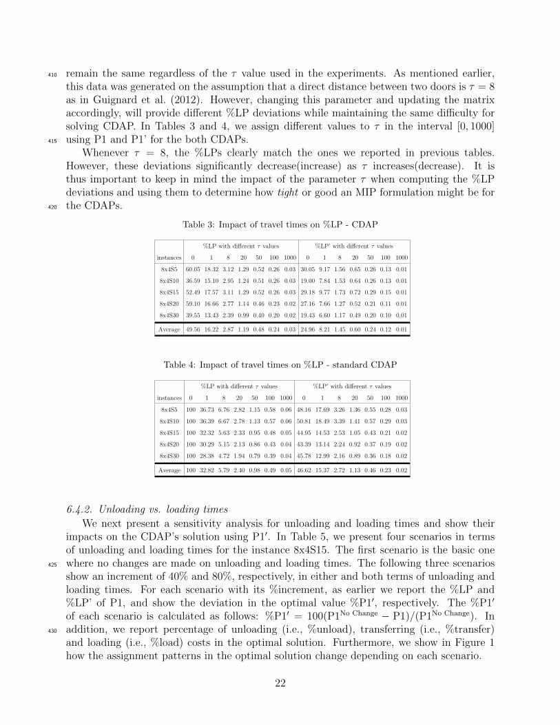
6.4.2. Unloading vs. loading times

We next present a sensitivity analysis for unloading and loading times and show theirimpacts on the CDAP’s solution using P1′. In Table 5, we present four scenarios in termsof unloading and loading times for the instance 8x4S15. The first scenario is the basic onewhere no changes are made on unloading and loading times. The following three scenarios425

show an increment of 40% and 80%, respectively, in either and both terms of unloading andloading times. For each scenario with its %increment, as earlier we report the %LP and%LP’ of P1, and show the deviation in the optimal value %P1′, respectively. The %P1′

of each scenario is calculated as follows: %P1′ = 100(P1No Change − P1)/(P1No Change). Inaddition, we report percentage of unloading (i.e., %unload), transferring (i.e., %transfer)430

and loading (i.e., %load) costs in the optimal solution. Furthermore, we show in Figure 1how the assignment patterns in the optimal solution change depending on each scenario.

22

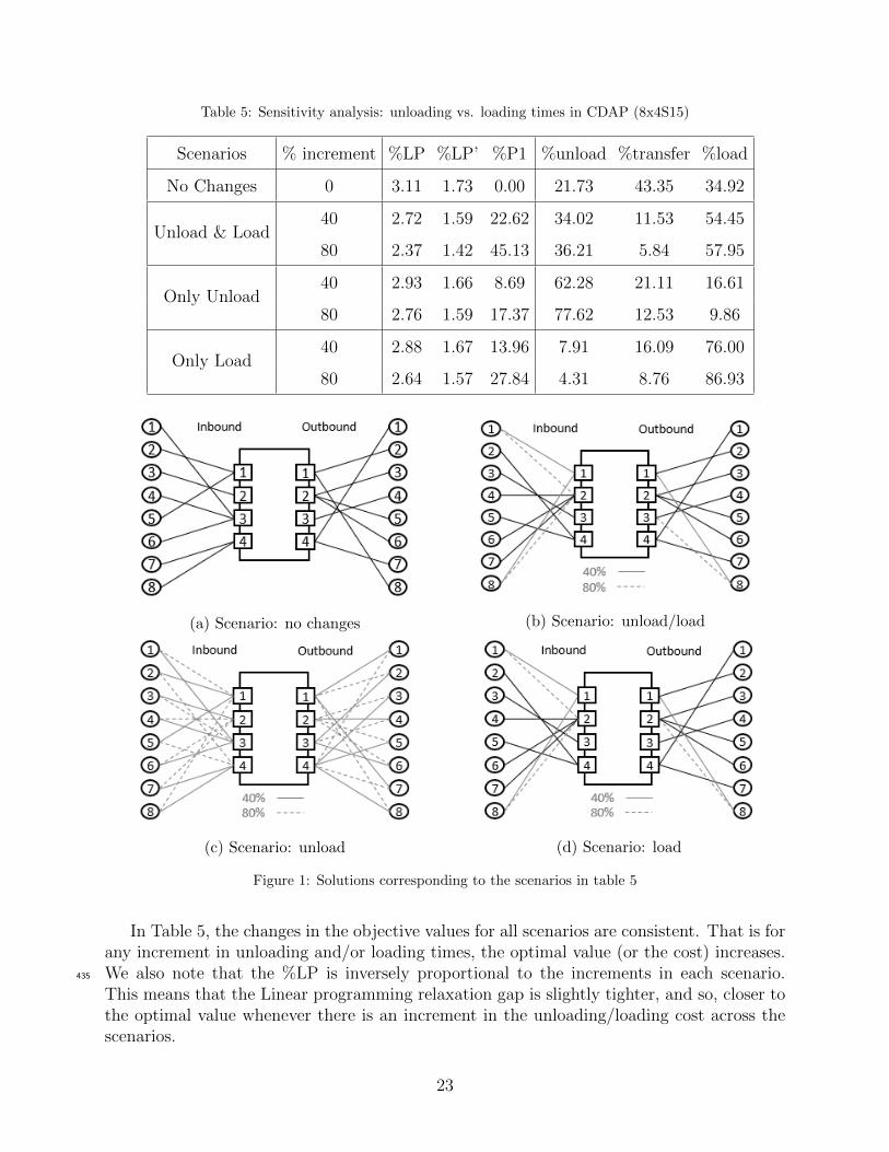
Table 5: Sensitivity analysis: unloading vs. loading times in CDAP (8x4S15)

Scenarios % increment %LP %LP’ %P1 %unload %transfer %load

No Changes 0 3.11 1.73 0.00 21.73 43.35 34.92

Unload & Load40 2.72 1.59 22.62 34.02 11.53 54.45

80 2.37 1.42 45.13 36.21 5.84 57.95

Only Unload40 2.93 1.66 8.69 62.28 21.11 16.61

80 2.76 1.59 17.37 77.62 12.53 9.86

Only Load40 2.88 1.67 13.96 7.91 16.09 76.00

80 2.64 1.57 27.84 4.31 8.76 86.93

(a) Scenario: no changes (b) Scenario: unload/load

(c) Scenario: unload (d) Scenario: load

Figure 1: Solutions corresponding to the scenarios in table 5

In Table 5, the changes in the objective values for all scenarios are consistent. That is forany increment in unloading and/or loading times, the optimal value (or the cost) increases.We also note that the %LP is inversely proportional to the increments in each scenario.435

This means that the Linear programming relaxation gap is slightly tighter, and so, closer tothe optimal value whenever there is an increment in the unloading/loading cost across thescenarios.

23

Figure 1 shows the assignment patterns in the optimal solution of CDAP for all scenariosin Table 5. We observe that the changes are minor in scenarios (b) and (d). However, the440

solution is completely different in (c), when unloading is increased from 40% to 80%.

6.4.3. Identical vs. non-identical door capacities

We next present a sensitivity analysis for the impact of doors’ capacities on the optimalvalue of CDAP. Consequently, we choose to present two cases: identical and non-identicalcapacities. In each case, we present the base value as its base capacity, and increase the base445

by a parameter φ, where φ = 0, 10%, 20%, 30%, 40%, 50%, 60%, 70%, 80%, 90%, 100%.For the first case of identical capacities, we select the instance 8x4S5 with its base value

being 159, and show in Figure 2a the changes in the optimal value with respect to theadditional capacity slackness. Similarly, for the second case of non-identical capacities, weselect the general instance 8x4 with its base value being randomly generated using a uniform450

distribution of U ∼ [159, 196]. The values 159 and 196 represent the minimum and maximumcapacities, respectively, for the instance 8x4. In our instance generation in section 6.1, 159was the identical capacity for 8x4S5 while 196 for 8x4S30, hence we chose to generate thenon-identical capacities within this range. We then show in Figure 2b the changes in theoptimal value with respect to the additional capacity slackness.455

In Figure 2, the optimal values with respect to both cases of identical and non-identicalcapacities are decreasing as the slackness is increasing. Such a behavior can be seen as theadditional or marginal cost saved of adding more resources to the cross-dock’s door. Thereis, however, no significant difference between having identical and non-identical capacities inthe optimal value.460

(a) identical capacities (b) non identical capacities

Figure 2: Changes in optimal value when capacity slackness is increased

7. Conclusions

In this paper we studied cross-dock door assignment problems with and without load-ing/unloading times. We presented two new mathematical programming formulations whichwere analytically and computationally compared with existing ones. In particular, we com-pared them with respect to the quality of their %LP and with respect to Lagrangean bounds465

24

presented in Nassief et al. (2016). We showed than the LP relaxation of the configurationbased formulation is equivalent to the Lagrangean Dual problem of the LR given in Nassiefet al. (2016). However, the results of computational experiments indicate that, when using acolumn generation algorithm instead of a subgradient optimization algorithm, better boundscan be obtained in practice. This behavior is mainly attributed to the slow convergence of the470

subgradient algorithm as compared to a CG for this particular class of problems. Althoughwe pointed out that the main contribution of this paper is theoretical while being supportedby some computational experiments, it is important to highlight that the applicability ofour methodologies are limited to a size of 20 origins, 20 destinations, 10 inbound and 10outbound doors. In practice, some cross-dock facilities have 6-8 doors while others can have475

up to 200 doors. To the best of our knowledge, the largest cross-dock in the world is toldto be in Dallas, TX with more than 500 doors as reported in Gue (1999). We also pointedout the impact of parameters used in the generation of travel times (or distances) betweendoors and the perceived quality of the LP bounds obtained with the formulations. Futureresearch may focus on polyhedral studies on some of the proposed formulations to identify480

families of valid inequalities that can improve the LP relaxation bounds.

8. Acknowledgments

The research of the first author is supported by the Ministry of Higher Education - SaudiArabia. The research of the second author was partly supported by the Natural Sciencesand Engineering Research Council of Canada under grant 418609-2012. The research of the485

third author has been supported by a Concordia University Research Chair (Tier I) andby an NSERC (Natural Sciences and Engineering Research Council of Canada) grant. Theauthors thank two anonymous reviewers for their valuable comments on a previous versionof this paper.

9. References490

Agustina, D., Lee, C., Piplani, R., 2010. A review: Mathematical models for cross dockingplanning. International Journal of Engineering Business Management 2 (2), 47 – 54.

Amini, A., Tavakkoli-Moghaddam, R., Omidvar, A., 2014. Cross-docking truck schedulingwith the arrival times for inbound trucks and the learning effect for unloading/loadingprocesses. Production & Manufacturing Research 2 (1), 784–804.495

Amor, H. M. B., Desrosiers, J., Frangioni, A., 2009. On the choice of explicit stabilizingterms in column generation. Discrete Applied Mathematics 157 (6), 1167–1184.

Bartholdi III, J. J., Hackman, S. T., 2011. Warehouse & distribution science: release 0.92.Atlanta, GA, The Supply Chain and Logistics Institute, School of Industrial and SystemsEngineering, Georgia Institute of Technology.500

Boysen, N., 2010. Cross dock scheduling: Classification, literature review and researchagenda. Omega 38 (6), 413 – 422.

25

Bozer, Y., Carlo, H., 2008. Optimizing inbound and outbound door assignments in less-than-truckload crossdocks. IIE Transactions 40 (11), 1007 – 1018.

Buijs, P., Vis, I., Carlo, H., 2014. Synchronization in cross-docking networks: A research505

classification and framework. European Journal of Operational Research 239 (3), 593 –608.

Chen, F., Song, K., 2009. Minimizing makespan in two-stage hybrid cross docking schedulingproblem. Computers & Operations Research 36 (6), 2066 – 2073.

Cohen, Y., Keren, B., 2009. Trailer to door assignment in a synchronous cross-dock operation.510

International Journal of Logistics Systems and Management 5 (5), 574 – 590.

Crainic, T.G., Frangioni, A., Gendron, B., 2001. Bundle-based relaxation methods formulticommodity capacitated fixed charge network design. Discrete Applied Mathemat-ics 112 (1), 73–99.

Enderer, F., Contardo, C., Contreras, I., 2017. Integrating dock-door assignment and vehicle515

routing with cross-docking. Computers & Operations Research 88, 30 – 43.

Forger, G., 1995. Ups starts world’s premiere cross-docking operation. Modern materialhandling 36 (8), 36 – 38.

Gelareh, S., Monemi, R. N., Semet, F., Goncalves, G., 2016. A branch-and-cut algorithm forthe truck dock assignment problem with operational time constraints. European Journal520

of Operational Research 249 (3), 1144 – 1152.

Geoffrion, A. M., 1974. Lagrangean relaxation for integer programming. Springer.

Gue, Kevin R, 1999. The effects of trailer scheduling on the layout of freight terminals.Transportation Science 33 (4), 419 – 428.

Guignard, M., Hahn, P., Pessoa, A. A., da Silva, D. C., 2012. Algorithms for the crossdock525

door assignment problem. In: Fourth International Workshop on Model-Based Metaheuris-tics. Brazil, pp. 1–12.

Kinnear, E., 1997. Is there any magic in cross-docking? Supply Chain Management: AnInternational Journal 2 (2), 49 – 52.

Ladier, A.-L., Alpan, G., 2016. Cross-docking operations: Current research versus industry530

practice. Omega 62, 145–162.

Li, Y., Pardalos, P., Ramakrishnan, K., Resende, M., 1994. Lower bounds for the quadraticassignment problem. Annals of Operations Research 50 (1), 387–410.

Maknoon, Y. and Laporte, G., 2017. Vehicle routing with cross-dock selection. Computers& Operations Research 77, 254 – 266.535

26

Maknoon, Y and Soumis, F. and Baptiste, P., 2017. An integer programming approach toscheduling the transshipment of products at cross-docks in less-than-truckload industries.Computers & Operations Research 82, 167 – 179.

Martello, S., Pisinger, D., Toth, P., 2000. New trends in exact algorithms for the 0–1 knapsackproblem. European Journal of Operational Research 123 (2), 325 – 332.540

Napolitano, M., 2011. Cross dock fuels growth at dots. Logistics management 50 (2), 30 –34.

Nassief, W., Contreras, I., As’ad, R., 2016. A mixed-integer programming formulation andlagrangean relaxation for the cross-dock door assignment problem. International Journalof Production Research 54, 494–508.545

Oh, Y., Hwang, H., Cha, C., Lee, S., 2006. A dock-door assignment problem for the koreanmail distribution center. Computers & Industrial Engineering 51 (2), 288 – 296.

Peck, K., 1983. Operational analysis of freight terminals handling less than container loadshipments. Ph.D. thesis, University of Illinois, Urbana-Champaign, IL, United States.

Sherali, H. D., Adams, W. P., 2013. Reformulation–linearization techniques for discrete550

optimization problems. In: Handbook of Combinatorial Optimization. Springer, pp. 2849–2896.

Shuib, A., Fatthi, W., 2012. A review on quantitative approaches for dock door assignmentin cross-docking. International Journal on Advanced Science, Engineering and InformationTechnology 2 (5), 30 – 34.555

Tsui, L., Chang, C.-H., 1990. A microcomputer based decision support tool for assigningdock doors in freight yards. Computers & Industrial Engineering 19 (1), 309 – 312.

Tsui, L., Chang, C.-H., 1992. An optimal solution to a dock door assignment problem.Computers & Industrial Engineering 23 (1), 283 – 286.

Van Belle, J., Valckenaers, P., Cattrysse, D., 2012. Cross-docking: State of the art. Omega560

40 (6), 827 – 846.

Witt, C., 1998. Crossdocking: Concepts demand choice. Material Handling Engineering53 (7), 44 – 49.

Zhang, T., Saharidis, G., Theofanis, S., Boile, M., 2010. Scheduling of inbound and outboundtrucks at cross-docks: Modeling and analysis. Transportation Research Record: Journal565

of the Transportation Research Board 2162, 9–16.

Zhu, Y., Hahn, P., Liu, Y., Guignard, M., 2009. New approach for the cross-dock doorassignment problem. In: Anais do XLI Simposio de Pesquisa Operacional. Porto Seguro,Bahia, Brazil, pp. 1226–1236.

27