a comparison of gaussian and mean curvature estimation ...ehudr/publications/pdf/magidsr07a.pdf ·...

www.elsevier.com/locate/cviu

Computer Vision and Image Understanding 107 (2007) 139–159

A comparison of Gaussian and mean curvature estimation methodson triangular meshes of range image data

Evgeni Magid, Octavian Soldea *, Ehud Rivlin

Computer Science Faculty, The Technion, Israel Institute of Technology, Haifa 32000, Israel

Received 22 June 2005; accepted 29 September 2006Available online 26 December 2006

Abstract

Estimating intrinsic geometric properties of a surface from a polygonal mesh obtained from range data is an important stage ofnumerous algorithms in computer and robot vision, computer graphics, geometric modeling, and industrial and biomedical engineering.This work considers different computational schemes for local estimation of intrinsic curvature geometric properties. Four different algo-rithms and their modifications were tested on triangular meshes that represent tessellations of synthetic geometric models. The resultswere compared with the analytically computed values of the Gaussian and mean curvatures of the non-uniform rational B-spline(NURBS) surfaces from which these meshes originated. The algorithms were also tested on range images of geometric objects. Theresults were compared with the analytic values of the Gaussian and mean curvatures of the scanned geometric objects. This work man-ifests the best algorithms suited for Gaussian and mean curvature estimation, and shows that different algorithms should be employed tocompute the Gaussian and mean curvatures.� 2006 Elsevier Inc. All rights reserved.

Keywords: Geometric modeling; Principal curvatures; Gaussian curvature; Mean curvature; Polygonal mesh; Triangular mesh; Range data

1. Introduction

A number of approaches have been proposed to repre-sent a 3D object for the purposes of reconstruction, recog-nition, and identification. The approaches are generallyclassified into two groups: volumetric- and boundary-basedmethods. A volumetric description utilizes global charac-teristics of a 3D object: principal axes, inertia matrix [25],tensor-based moment functions [13], differential character-istics of iso-level surfaces [35,50], etc. Boundary-basedmethods describe an object based on distinct local proper-ties of its boundary and their relationships. This method iswell suited for recognition purposes because local proper-ties are still available when only a partial view of an objectis acquired.

1077-3142/$ - see front matter � 2006 Elsevier Inc. All rights reserved.

doi:10.1016/j.cviu.2006.09.007

* Corresponding author.E-mail address: [email protected] (O. Soldea).

Differential invariant properties such as Gaussian andmean curvatures are one of the most essential features inboundary-based methods, extensively used for segmenta-tion, recognition, and registration algorithms [2,57]. Unfor-tunately, these significant geometric quantities are definedonly for twice differentiable (C2) surfaces. In contrast, geo-metric data sets are frequently available as polygonal,piecewise linear approximations, typically as triangularmeshes. Such data sets are common output of, for exam-ples, 3D scanners.

A plethora of work [1,5,11,20,24,28,30,31,33,34,42,44,49,54] describing algorithms for curvature estimationfrom polygonal surfaces exists. Great effort has beeninvested in designing methods of computing curvature thattarget real range image data [3,52]. The existence of such alarge number of curvature computation methods made itnecessary to find some way of comparing them[15,22,27,44,46,51]. Unfortunately, although error analysismethods for several different algorithms exist [33,34], theknown comparison results are insufficient and provide only

mailto:[email protected]

140 E. Magid et al. / Computer Vision and Image Understanding 107 (2007) 139–159

a partial image. The reason for the absence of such workmay lie in the large amount of factors that has to be ana-lyzed when comparing curvature. A few examples of suchfactors are finding interesting, representative, and fair sur-faces for computing curvatures, developing a reliable wayof evaluating the accuracy of computations, and, neverthe-less, the time and memory requirements of differentmethods.

Starting in the 1980s, the curvature computation fieldmade great strides. Probably the first comparison workwas published in 1989, [15]. The authors’ conclusion wasthat the algorithms existing at that time were appropriatefor computing the signs of the curvatures, while the valuesof the curvatures were extremely sensitive to quantizationnoise. In this context, the authors in [52] reached the sameconclusion six years later, in 1995.

Recently, methods providing the ability to compute cur-vature values are reported in literature. They can begrouped into several main approaches. A good and updat-ed characterization of the existing literature can be foundin [51]. Following [51], we describe the most common cur-vature computation methods.

1.1. Methods employing local analytic surface

approximations

Curvature computation essentially means evaluations ofsecond order derivatives [7]. This process is known to besensitive to quantization noise. Probably the most popularapproach for trying to cope with this phenomenon com-putes an approximation of the vicinity of a node with ananalytic surface. In general, quadratic or cubic surfacesare involved. To the best of our knowledge, the most pop-ular approach is paraboloid fitting together with its vari-ants [20,27,28,42,44].

A lot of effort has been invested in finding good localapproximation surfaces. A comparison of local surfacegeometry estimation methods in terms of accuracy compu-tation of curvatures can be found in [32].

Several extensions of the paraboloid fitting methodswere also proposed in [14,17,29,40]. We mention that thereare methods that employ local analytic surface approxima-tions via computing nearly isometric parameterizations foreach vertex [41] and via a spline surface fitting stage [36].

1.2. Methods employing discrete approximation formulas

Discrete approximation formulas employ the 3D infor-mation existent in a node and its neighbors in a direct for-mula. In general, the formulas used are relatively short, afact that provides some gain in computation time at thecost of the attainable accuracy. The authors in [24,27,33]considered such methods based on the Gauss–Bonnet[9,45] theorem. We describe such a method, that is basedon the Gauss–Bonnet theorem, in detail in Section 3.2.

In this context, the Gauss–Bonnet theorem can be usedon simplex meshes [8], which are representations consid-

ered to be topologically dual to triangulations. Moreover,applications of angle excess in the context of minimal sur-faces and straight geodesics can be found in [38,39].

1.3. Methods employing Euler and Meusnier theorems

In numerous works, curvature computation is based onevaluating the curvature of curves that cross through a ver-tex and its neighbors. Each neighbor provides a directionalcurvature value. These values are further merged employ-ing Euler and Meusnier theorems (see [9,45]). In manyother works, curvature computation is based on approxi-mating tangent circles to surfaces. In this context, in[5,31], circular cross sections, near the examined vertex,are fitted to the surface. Then, the principal curvaturesare computed using Meusnier and Euler theorems (see[9,45]). An interesting application of the Euler theoremtoward curvature computation can be found in [54]. Wedescribe this method in detail in Section 3.3.

1.4. Methods employing tensor evaluations

The tensor curvature is a map that associates to eachsurface tangent direction (at a surface point) the corre-sponding directional curvature (see [49] for details). Proba-bly the most popular method for curvature computationsbased on tensor curvature evaluation is [49]. Note that anextension of the Taubin scheme [49] appears in [19]. Gopiet al. [19] employs extended regions on neighbors and usesa different weighting scheme.

1.5. Methods employing voting mechanisms

Besides extended regions of neighbors, and closely relat-ed to, voting mechanisms are often employed towards algo-rithms accuracy improvement. The authors feel that mostof the voting mechanisms existent in the literature, targetedthe tensor computation accuracy improvement. In this con-text, Taubin approach [49] is at center stage and severalvery interesting improvements were reported as follows.

A method considered to be robust to noise when evalu-ating the signs of curvatures [51] can be found in [47]. Fol-lowing [47] and [48], the authors in [37] proposed animprovement over Taubin’s method [49] that, in addition,detects crease values over large meshes. Another improve-ment in the quality of curvature computation was recentlyreported in [51].

1.6. Methods employing multi-scaling and total and global

techniques

Relative recent works investigated the developing oflocal surface descriptors that employ smoothing and filter-ing at different scales toward reliable curvature computa-tion. Probably the most representative method in themulti-scaling methods category is [34]. The results achievedin [34] are dependent on a 2D Gaussian filtering iteratively

E. Magid et al. / Computer Vision and Image Understanding 107 (2007) 139–159 141

applied on the input free-form. An estimation of the erroris also provided [34]. Note that the advantage of multi-scaletechniques is that they provide solutions for multi-targetproblems, such as interpolation, smoothing, and segmenta-tion simultaneously [10].

The authors in [37] identified a category of curvaturecomputation methods that provides the values of curva-tures at each point at the end of the computations. In thisapproach, intermediate computation stages have to be fin-ished over the entire input in order to be able to evaluatethe curvature values at any point of interest. This approachis used in [56], where the authors proposed a method forcomputing the electrical charge distributions of a field tar-geting segmentation. The electrical charge distribution is,in fact, a differential characteristic that is proven to havesimilar properties to the curvature, especially for segmenta-tion tasks.

1.7. Choosing methods for comparison

Following [46], we attempt to quantitatively comparefour methods for estimating the Gaussian and mean curva-tures of triangular meshes. We tested these methods on tri-angular meshes that represent tessellations of foursynthetically generated objects: a cylinder, a cone, a sphere,and a plane, as well as on non-uniform rational B-spline(NURBS) surfaces. The results are compared to the analyt-ic evaluation of these curvature properties on the surfaces.Moreover, we present the results of tests of the perfor-mance of the different methods on range images of geomet-ric objects scanned using a 3D Cyberware scanner [23]. Theresults are compared to the analytic values of the Gaussianand mean curvatures of the scanned geometric objects. Theanalytic values of the Gaussian and mean curvatures wereinferred from the dimensions of the real objects. Thedimensions of the objects were measured using amicrometer.

In our experiments, we employed four synthetically gen-erated objects and their real objects counterparts, whichhave similar dimensions and tessellations. This fact repre-sents a key factor in our comparisons.

Our main goal is to obtain a high level of understandingof the main current approaches. In order to obtain suchinsight, we selected four specific methods, each one repre-sentative of a different approach. The chosen methodsare: paraboloid fitting (Section 3.1), Gauss–Bonnet (Sec-tion 3.2), Watanabe and Belayev (Section 3.3), and Taubin(Section 3.4).

1.7.1. Methods employing local analytic surface

approximations: paraboloid fitting

We feel that paraboloid fitting is an appropriate repre-sentative method, it being by far the most popular methodof its class. In [27] and [44] the paraboloid fitting method iscompared to other ones. The authors in [27] provide us ageneral overview of three algorithms on four types of prim-itive surfaces: spheres, planes, cylinders, and trigonometric

surfaces. No general surfaces are considered, however. In[44], five methods are compared on a cube, a sphere, anoisy sphere, and an approximated image of a ventricle.

1.7.2. Methods employing discrete approximations formulas:

the Gauss–Bonnet scheme

In [24,27,33], an algorithm based on the Gauss–Bonnettheorem [9,45] is described. We refer to it as the Gauss–Bonnet scheme. The Gauss–Bonnet scheme is also knownas the angle deficit method [33]. The authors in [33] providean error analysis for this method. The reasons for choosingthe Gauss–Bonnet scheme is that it is extremely popular forcomputing the Gaussian curvature and both the Gaussianand mean curvatures involve a convenient, elegant, andfast evaluation of a formula based on turning the anglesof its neighbors.

1.7.3. Methods employing Euler and Meusnier theorems: the

Watanabe and Belyaev approach

Numerous methods of curvature computation employEuler and Meusnier theorems [9,45]. We have chosen theWatanabe and Belyaev scheme [54] as representative of thisgroup. The authors in [54] focused on mesh decimation,and provide a comparison of mesh decimation methods.Unfortunately, there is no mention of the accuracy of thecurvature computation the authors proposed. The reasonfor choosing the Watanabe and Belyaev scheme is that,in our opinion, its performance primarily as regards curva-ture computation accuracy is unknown. Specifically, [31]concluded that the paraboloid fitting provides better resultsthan a method that involves Euler and Meusnier theorems,called the circular cross sections method, on noisy data. Wemention that the interest in analyzing the Watanabe andBelyaev scheme comes also from its behavior on noisy datacaptured in range images of real 3D objects as we show inSection 4.2.

1.7.4. Methods employing tensor evaluations and voting

mechanisms: the Taubin approachOur belief is that the method that best fits the tensor

evaluating methodology is Taubin’s method. Moreover,the vast majority of algorithms that attempt improvementsof curvature computation accuracy by voting target tensorevaluation and, therefore, the Taubin method. Anotherbenefit of Taubin’s method is that it provides very goodresults and was tested on real objects; see [21].

The paper is organized as follows: a short review of dif-ferential geometry of surfaces is provided in Section 2. InSection 3, a concise description of the four algorithms weconsidered is given. Then, results of our comparison arepresented in Section 4. Finally, we conclude in Section 5.

2. Differential geometry of surfaces

Let ~Sðx; yÞ be a regular C2 continuous freeform para-metric surface in R3. The unit normal vector field of~Sðx; yÞ is defined by


~Nðx; yÞ ¼oox~Sðx; yÞ � o

oy~Sðx; yÞ

oox~Sðx; yÞ � o

oy~Sðx; yÞ

�� :The curvature j of curve ~CðtÞ : ½a; b� ! S passing throughthe point ~Sðx0; y0Þ ¼ ~Cðt0Þ is defined by

j ¼ j~C0ðt0Þ � ~C00ðt0Þjh~C0ðt0Þ; ~C0ðt0Þi3=2

;

where a, b 2 R and ÆÆ, Ææ is the scalar product of vectors.The normal curvature jn of curve ~C �~S passing through

the point ~Sðr0; t0Þ is defined by the following relation,known as

Theorem 2.1 (Meusnier’s theorem).

jn ¼ j cos u; ð2:1Þwhere j is the curvature of ~C at ~Sðr0; t0Þ and u is the angle

between the curve’s normal n and the normal ~Nðr0; t0Þ of ~S.

A graphical representation of Meusnier theorem can beseen in Fig. 1.

The principal curvatures, j1(r0, t0) and j2(r0, t0), of ~S at~Sðr0; t0Þ are defined as the maximum and minimum normalcurvatures at ~Sðr0; t0Þ, respectively. The directions forwhich these values are attained are called the principal

directions (see [9,45]). We denote the principal directionswith P1 and P2, respectively. Bearing in mind that Meus-nier’s theorem associates to each direction a normal curva-ture at each surface point ~Sðr0; t0Þ; the definitions ofprincipal curvatures and directions are consistent. The nor-mal curvature jn of surface ~Sðr; tÞ in tangent direction ~T isequal to:

Theorem 2.2 (Euler’s theorem).

jn ¼ j1 cos2 hþ j2 sin2 h; ð2:2Þwhere h is the angle between the first principal direction and~T .

Fig. 1. Curvature and normal curvature at a point on a curve on a surface.k is the curvature of C at v,~n is the curvature of C at v, ~N is the normal tothe surface S at v, kn is the normal curvature at v, and k~n is a vectororiented in the direction of ~n with length 1

k.

The Gaussian and mean curvatures, K(r,t) and H(r,t),are uniquely defined by the principal curvatures of thesurface:

Kðr; tÞ ¼j1ðr; tÞ � j2ðr; tÞ; ð2:3Þ

Hðr; tÞ ¼ j1ðr; tÞ þ j2ðr; tÞ2

: ð2:4Þ

3. Algorithms for curvature estimation

In this work, we consider four methods for the estima-tion of the Gaussian and mean curvatures, for triangularmeshes. We assume that each given triangular meshapproximates a smooth, at least twice differentiable,surface.

3.1. Paraboloid fitting

The paraboloid fitting method, as well as several vari-ants of it, were described in [20,27,28,42,44]. In[20,27,28,42,44], the principal curvatures and principaldirections of a triangulated surface are estimated at eachvertex by a least squares fitting of an osculating paraboloidto the vertex and its neighbors. These references use linearapproximation methods where the approximated surface isobtained by solving an over-determined system of linearequations. More recently, in [33], the authors provided anasymptotic analysis of the paraboloid fitting scheme adapt-ed to an interpolation case.

Interestingly enough, the paraboloid fitting method wasconsidered a good estimator for differential parameter esti-mation in iterative processes. For example, in [42], theauthors presented a nonlinear functional minimizationalgorithm that is implemented as an iterative constraintsatisfaction procedure based on local surface smoothnessproperties.

The paraboloid fitting algorithm approximates a smallneighborhood of the mesh around a vertex v by an osculat-ing paraboloid. The principal curvatures of the surface areconsidered to be identical to the principal curvatures of theparaboloid (see [20,27,28,42,44]).

Vertex vi is considered an immediate neighbor of vertexv if edge ei ¼ vvi belongs to the mesh. Denote the set ofimmediate neighboring vertices of v by fvign�1

i¼0 and the setof the triangles containing the vertex v by fDv

i gn�1i¼0 ,

Dvi ¼ Mðvi v vðiþ1Þmod nÞ; 0 6 i 6 n� 1: ð3:1Þ

Fig. 2 shows the notations used for vertices, edges, andtriangles.

Let ~N v be the normal of surface ~S at vertex v. Normalsare, in many cases, provided with the mesh in order toenable Gouraud and/or Phong shading [16]. Otherwise, let

~Nvi ¼

ðvi � vÞ � ðvðiþ1Þmod n � vÞkðvi � vÞ � ðvðiþ1Þmod n � vÞk ; ð3:2Þ

be the unit normal of triangle Dvi . Then, ~Nv could be esti-

mated as an average of normals ~Nvi :

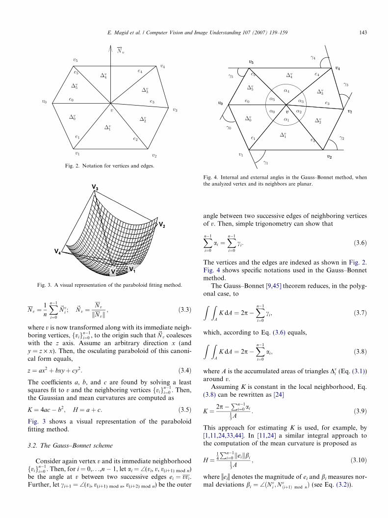
Fig. 4. Internal and external angles in the Gauss–Bonnet method, whenthe analyzed vertex and its neighbors are planar.

Fig. 2. Notation for vertices and edges.

Fig. 3. A visual representation of the paraboloid fitting method.


Nv ¼1

n

Xn�1

i¼0

~Nvi ;

~Nv ¼Nv

kNvk; ð3:3Þ

where v is now transformed along with its immediate neigh-boring vertices, fvign�1

i¼0 , to the origin such that ~N v coalesceswith the z axis. Assume an arbitrary direction x (andy = z · x). Then, the osculating paraboloid of this canoni-cal form equals,

z ¼ ax2 þ bxyþ cy2: ð3:4Þ

The coefficients a, b, and c are found by solving a leastsquares fit to v and the neighboring vertices fvign�1

i¼0 . Then,the Gaussian and mean curvatures are computed as

K ¼ 4ac� b2; H ¼ aþ c: ð3:5Þ

Fig. 3 shows a visual representation of the paraboloidfitting method.

3.2. The Gauss–Bonnet scheme

Consider again vertex v and its immediate neighborhoodfvign�1

i¼0 . Then, for i = 0,. . .,n � 1, let ai = \(vi, v, v(i+1) mod n)be the angle at v between two successive edges ei ¼ vvi.Further, let ci+1 = \(vi, v(i+1) mod n, v(i+2) mod n) be the outer

angle between two successive edges of neighboring verticesof v. Then, simple trigonometry can show that

Xn�1

i¼0

ai ¼Xn�1

i¼0

ci: ð3:6Þ

The vertices and the edges are indexed as shown in Fig. 2.Fig. 4 shows specific notations used in the Gauss–Bonnetmethod.

The Gauss–Bonnet [9,45] theorem reduces, in the polyg-onal case, to

Z ZA

K dA ¼ 2p�Xn�1

i¼0

ci; ð3:7Þ

which, according to Eq. (3.6) equals,

Z ZA

K dA ¼ 2p�Xn�1

i¼0

ai; ð3:8Þ

where A is the accumulated areas of triangles Dvi (Eq. (3.1))

around v.Assuming K is constant in the local neighborhood, Eq.

(3.8) can be rewritten as [24]

K ¼ 2p�Pn�1

i¼0 ai13A

: ð3:9Þ

This approach for estimating K is used, for example, by[1,11,24,33,44]. In [11,24] a similar integral approach tothe computation of the mean curvature is proposed as

H ¼14

Pn�1i¼0 keikbi

13A

; ð3:10Þ

where ieii denotes the magnitude of ei and bi measures nor-mal deviations bi ¼ \ðNv

i ;Nvðiþ1Þ mod nÞ (see Eq. (3.2)).


3.3. The Watanabe and Belyaev approach

A simple method for estimating the principal curvaturesof a surface that is approximated by a triangular mesh wasproposed in [54].

Consider an oriented surface ~S. Let ~T be a tangent vec-tor and ~N be the unit normal at a surface point v. A normalsection curve ~rðsÞ associated with ~T at v is defined as theintersection between the surface and the plane through v

that is spanned by ~T and ~N (see Fig. 5). Let ~P 1 and ~P 2 bethe principal directions at v associated with the principalcurvatures j1 and j2, respectively. jn(u) denotes the nor-mal curvature of the normal section curve, where u is theangle between ~T and ~P 1. Using Euler’s theorem (see Theo-rem 2.2), integral formulas of jn(u) and its square arederived [54]:

1

2p

Z 2p

0

knðuÞdu ¼ H ;1

2p

Z 2p

0

knðuÞ2 du ¼ 3

2H 2 � 1

2K:

ð3:11Þ

In order to estimate the integrals of Eq. (3.11), one needs toestimate the normal curvature around v, in all possible tan-gent directions.

Consider v being a mesh vertex and recall its normal ~Nv

(Eq. (3.3)). Here, the average of the normals of the facesadjacent to vertex v takes into account the relative areasof the different faces.

v is now transformed along with its immediate neighbor-ing vertices, fvign�1

i¼0 , to the origin such that ~Nv coalesceswith the z axes. Consider the intersection curve ~r ¼~rðsÞof the surface by a plane through v that is spanned by Nv

(the z axis in our canonical form) and edge ei ¼ vvi. A Tay-lor series expansion of~rðsÞ gives

~rðsÞ ¼~rð0Þ þ s~r0ð0Þ þ s2

2~r00ð0Þ þ � � �

¼~rð0Þ þ s~T r þs2

2jn~N r þ � � � ; ð3:12Þ

Fig. 5. Specific notations in the Watanabe and Belyaev method.

where Tr and Nr are the unit tangent and normal of r(s).Recall that v = r(0) and that vi = r(s). The arclength s couldbe approximated by the length of edge ei ¼ vvi, ors � kvvik. Multiplying Eq. (3.12) by ~N v ¼ ~N r yields,

~Nv � vvi � jnkvvik2

2; jn �

2~Nv � vvi

kvvik2: ð3:13Þ

The vertices and the edges are indexed as shown in Fig. 2.Fig. 5 shows specific notations used in the Watanabe andBelyaev method.

The trapezoid approximation of Eq. (3.11) leads to

2pH �Xn�1

i¼0

jin

aði�1Þmod n þ ai

2

� �ð3:14Þ

and

2p3

2H 2 � 1

2K

� ��Xn�1

i¼0

kin

2 aði�1Þmod n þ ai

2

� �: ð3:15Þ

3.4. The Taubin approach

Let ~P 1 and ~P 2 be the two principal directions at point v

of surface~S and let ~T h ¼ ~P 1 cosðhÞ þ~P 2 sinðhÞ be some unitlength tangent vector at v. Taubin, in [49], defines the sym-metric matrix Mv by the integral formula of

Mv ¼1

2p

Z þp

�pjv

nð~T hÞ~T h~T T

h dh; ð3:16Þ

where jvnð~T hÞ is the normal curvature of S at v in the direc-

tion ~T h.Since the unit length normal vector ~N to ~S at v is an

eigenvector of Mv associated with the eigenvalue zero, itfollows that Mv can be factorized as follows

Mv ¼MT12

m11v m12

v

m21v m22

v

!M12; ð3:17Þ

where M12 ¼ ½~P 1;~P 2� is the 3 · 2 matrix constructed by con-catenating the column vectors ~P 1 and ~P 2. Note thatmij

v ¼MTijMvMij for any i, j 2 {1,2}. The principal curva-

tures can then be obtained as functions of the nonzeroeigenvalues of Mv [49]:

k1 ¼ 3m11v � m22

v ; k2 ¼ 3m22v � m11

v : ð3:18Þ

The first step of the implementation estimates the normalvector ~N v at each vertex v of the surface with the help ofEq. (3.2). Then, for each vertex v, matrix Mv is approximat-ed with a weighted sum over the neighbor vertices vi:

~Mv ¼Xn�1

i¼0

wijnð~T iÞ~T i~T T

i ; ð3:19Þ

where

~T i ¼ðI� ~Nv

~N Tv Þðv� viÞ

kðI� ~Nv~NT

v Þðv� viÞkð3:20Þ


is the unit length normalized projection of vector vi�v ontothe tangent plane h~N vi?. The normal curvature in direction~T i is approximated with the help of Eq. (3.13) as

jnð~T iÞ ¼ 2~NTv ðvi�vÞkvi�vk2 . The vertices and the edges are indexed

as shown in Fig. 2.The weights wi are selected to be proportional to the

sum of the surface areas of the triangles incident to bothvertices v and vi (two triangles if the surface is closed,and one triangle if both vertices belong to the boundaryof S).

By construction, the normal vector ~Nv is an eigenvectorof the matrix ~Mv associated with the eigenvalue zero. Then,~Mv is restricted to the tangent plane h~Nvi? and, using a

Householder transformation [18] and a Givens rotation[18], the remaining eigenvectors ~P 1 and ~P 2 of ~Mv (i.e., theprincipal directions of the surface at v) are computed.Finally, the principal curvatures are obtained from thetwo corresponding eigenvalues of ~Mv using Eq. (3.18).

1 The synthetic models along with their dimensions and curvature valuesfor each vertex (where is relevant) are also available in http://www.cs.technion.ac.il/~octavian/poly_crvtrs/poly_synthetic_data.

3.5. Modifications

We suggest several modifications for the paraboloid fit-ting [20,27,28,42,44], Watanabe and Belyaev [54], and Tau-bin [49] methods. We now describe our proposedmodifications.

We employed the paraboloid fitting method[20,44,42,28,27] on the rings of immediate neighbors (see[12] for a free implementation). Moreover, we extendedthese rings to neighbors that are not immediate. We referto the paraboloid fitting n method when rings from 1 upto n were involved in computations.

We considered two modifications to the algorithm ofWatanabe and Belyaev [54]. In the following two modifiedalgorithms, we do not change the first step of the Watanabeand Belyaev method. We employ the tangent directions ~T i

at vertex v produced by Eq. (3.20). Having two vertices (vand vi), tangent direction ~T i and the normal in v, we com-pute the radius of the fitted circle and from that derivejn(ui), the normal curvature in the specified direction ~T i.

• Watanabe A: Having the normal curvatures, we applyEqs. (3.14) and (3.15).

• Watanabe B: From the set of the normal curvatures ofeach vertex v, fji

ngn�1i¼0 , we select the maximal (k1) and

the minimal (k2) normal curvature values and applythe classic Eqs. (2.3) and (2.4).

We also considered two modifications of Taubin’s algo-rithm [49]:

• Taubin A (Constant integration): In Eq. (3.19), theweights wi are selected to be proportional to angles\ðvi; v; viþ1Þ instead of the surface areas.

• Taubin B (Smoothing with a trapezoidal rule): The direc-tional curvature jnð~T iÞ in Eq. (3.19) is selected as anaverage of values jnð~T ði�1Þmod nÞ and jnð~T iÞ.

4. Experimental results

We differentiate between two categories of data: syntheticand real range. While the interest for the synthetic data isgenerated from the fact that it is accurate and allows forground truth to be produced at any point, the interest inrange data is motivated by the fact that in most cases itis noisy, with direct influence on the accuracy and stabilityof the algorithms.

Denote by Ki and Hi the values of Gaussian and meancurvatures computed by one of the methods from the trian-gular mesh data in vertex vi, while Ki and Hi are the exact(analytically computed) values of the Gaussian and meancurvatures, at the same surface location vi ¼~Sðri; tiÞ onthe corresponding surface. We considered the followingerror values:

(1) Average of the absolute error value of the Gaussiancurvature K

1

m

Xm

i¼1

jKi � Kij;

(2) Average of the absolute error value of the square ofthe mean curvature H2

1

m

Xm

i¼1

jH 2i � H 2

i j:

4.1. Comparison using synthetic data

We tested all the algorithms described in Section 3 on aset of synthetic models that represent the tessellations offour objects: a cylinder, a conus, a sphere, and a plane.Moreover, we tested all the algorithms described in Section3 on a set of synthetic models that represent the tessella-tions of four NURBS surfaces: a surface of revolution gen-erated by a non-circular arc, the body and the spout ofthe infamous Utah teapot model, and an ellipsoid (seeFig. 7)1.

We built a library of triangular meshes that representapproximations (with different resolutions) of the syntheticmodels. For each synthetic surface, we have produced sev-eral polyhedral approximations with a varying number oftriangles. The cylinder, the cone, the sphere, and the planewere created artificially and ray-traced as if they werescanned (see Fig. 6).

Consider the way in which the Cyberware range scannercaptures 3D objects. This device registers the distances of3D points to the sensors. The sensors are situated at fixedpoints in a vertical line, relative to the ground. The cap-tured object is located at a platform that moves linearlyin the front of the sensors. The sensors are activated at

http://www.cs.technion.ac.il/~octavian/poly_crvtrs/poly_synthetic_data

http://www.cs.technion.ac.il/~octavian/poly_crvtrs/poly_synthetic_data

Table 1Dimensions of the cylinder, the cone, the sphere, and the plane in millimeters and their implicit analytic curvature values used in comparisons

K H2

Cylinder Radius = 33.25 0 0.015037594Cone Small radius = 24 Big radius = 50 Height = 150 0Sphere Radius = 19.8 0.00255076 0.00255076Plane Width Length 0 0

Fig. 6. The tessellations types of the synthetic counterparts of the real objects shown in Fig. 17, at relative low resolutions. The captured interior points aregrouped in square-like neighborhoods. The tessellation enriches these grouping with diagonal lines.


constant intervals of times, therefore, range images areparameterizable 3D sets of points. The directions ofparameterizations are two: the first is defined by the loca-tions where the sensors are activated, while the second isdefined by the density of the sensors on the vertical linethey are located at. The vast majority of interior pointsare captured in square-like neighborhoods. In Fig. 6, weshow the square-like neighborhood simulation resultstogether with diagonals added for triangulations buildingpurposes.

The dimensions and the analytic curvature values for thecylinder, the cone, the sphere, and the plane are specified inmillimeters in Table 1. The tessellations for the NURBS sur-faces was performed using samplings in the parametricdomain followed by evaluations of the 3D values on surfaces.The library files contain, for each NURBS surface and foreach vertex vi, its 3D coordinates and analyticallyprecomputed values of the Gaussian curvature Ki and the

Fig. 7. The NURBS surfaces that were

squared value of the mean curvature H 2i . The Gaussian

and mean curvature values are computed from the originalNURBS surfaces.

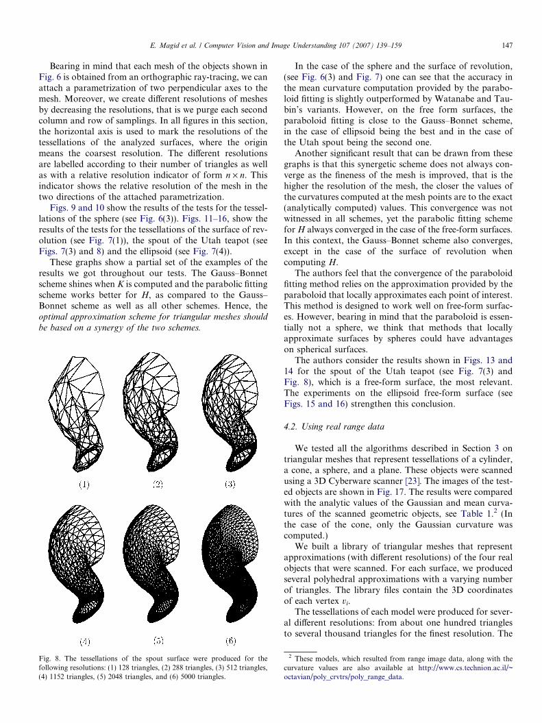
The tessellations of each model were produced for sever-al different resolutions: from about one hundred trianglesto several thousand triangles for the finest resolution. Thedifferent tessellations of the spout surface are shown inFig. 8. These different resolutions helped us gain someinsight into the convergence rates of the tested algorithmsas the accuracy of the tessellation improves.

In the vast majority of the previous results, only primi-tives such as cones and spheres were examined for the accu-racy of these curvature approximation algorithms. Theoutput of the tests of four different schemes on seven mod-els (see Figs. 6 and 7) shows that while the best algorithmfor the estimation of the Gaussian curvature is the Gauss–Bonnet scheme, the best method for the estimation of themean curvature is the paraboloid fitting method.

used for curvature estimation tests.


Bearing in mind that each mesh of the objects shown inFig. 6 is obtained from an orthographic ray-tracing, we canattach a parametrization of two perpendicular axes to themesh. Moreover, we create different resolutions of meshesby decreasing the resolutions, that is we purge each secondcolumn and row of samplings. In all figures in this section,the horizontal axis is used to mark the resolutions of thetessellations of the analyzed surfaces, where the originmeans the coarsest resolution. The different resolutionsare labelled according to their number of triangles as wellas with a relative resolution indicator of form n · n. Thisindicator shows the relative resolution of the mesh in thetwo directions of the attached parametrization.

Figs. 9 and 10 show the results of the tests for the tessel-lations of the sphere (see Fig. 6(3)). Figs. 11–16, show theresults of the tests for the tessellations of the surface of rev-olution (see Fig. 7(1)), the spout of the Utah teapot (seeFigs. 7(3) and 8) and the ellipsoid (see Fig. 7(4)).

These graphs show a partial set of the examples of theresults we got throughout our tests. The Gauss–Bonnetscheme shines when K is computed and the parabolic fittingscheme works better for H, as compared to the Gauss–Bonnet scheme as well as all other schemes. Hence, theoptimal approximation scheme for triangular meshes should

be based on a synergy of the two schemes.

Fig. 8. The tessellations of the spout surface were produced for thefollowing resolutions: (1) 128 triangles, (2) 288 triangles, (3) 512 triangles,(4) 1152 triangles, (5) 2048 triangles, and (6) 5000 triangles.

In the case of the sphere and the surface of revolution,(see Fig. 6(3) and Fig. 7) one can see that the accuracy inthe mean curvature computation provided by the parabo-loid fitting is slightly outperformed by Watanabe and Tau-bin’s variants. However, on the free form surfaces, theparaboloid fitting is close to the Gauss–Bonnet scheme,in the case of ellipsoid being the best and in the case ofthe Utah spout being the second one.

Another significant result that can be drawn from thesegraphs is that this synergetic scheme does not always con-verge as the fineness of the mesh is improved, that is thehigher the resolution of the mesh, the closer the values ofthe curvatures computed at the mesh points are to the exact(analytically computed) values. This convergence was notwitnessed in all schemes, yet the parabolic fitting schemefor H always converged in the case of the free-form surfaces.In this context, the Gauss–Bonnet scheme also converges,except in the case of the surface of revolution whencomputing H.

The authors feel that the convergence of the paraboloidfitting method relies on the approximation provided by theparaboloid that locally approximates each point of interest.This method is designed to work well on free-form surfac-es. However, bearing in mind that the paraboloid is essen-tially not a sphere, we think that methods that locallyapproximate surfaces by spheres could have advantageson spherical surfaces.

The authors consider the results shown in Figs. 13 and14 for the spout of the Utah teapot (see Fig. 7(3) andFig. 8), which is a free-form surface, the most relevant.The experiments on the ellipsoid free-form surface (seeFigs. 15 and 16) strengthen this conclusion.

4.2. Using real range data

We tested all the algorithms described in Section 3 ontriangular meshes that represent tessellations of a cylinder,a cone, a sphere, and a plane. These objects were scannedusing a 3D Cyberware scanner [23]. The images of the test-ed objects are shown in Fig. 17. The results were comparedwith the analytic values of the Gaussian and mean curva-tures of the scanned geometric objects, see Table 1.2 (Inthe case of the cone, only the Gaussian curvature wascomputed.)

We built a library of triangular meshes that representapproximations (with different resolutions) of the four realobjects that were scanned. For each surface, we producedseveral polyhedral approximations with a varying numberof triangles. The library files contain the 3D coordinatesof each vertex vi.

The tessellations of each model were produced for sever-al different resolutions: from about one hundred trianglesto several thousand triangles for the finest resolution. The

2 These models, which resulted from range image data, along with thecurvature values are also available at http://www.cs.technion.ac.il/~octavian/poly_crvtrs/poly_range_data.

http://www.cs.technion.ac.il/~octavian/poly_crvtrs/poly_range_data

http://www.cs.technion.ac.il/~octavian/poly_crvtrs/poly_range_data

Fig. 9. Average of the absolute error for the value of the Gaussian curvature for the tessellations of the sphere (see Fig. 6(3)). The Gauss–Bonnet scheme isthe most accurate being closely followed by the paraboloid fitting method.

Fig. 11. Average of the absolute error for the value of the Gaussian curvature for the tessellations of a surface of revolution (see Fig. 7(1)). The Gauss–Bonnet and the paraboloid fitting schemes provide the best accuracy, they having decreasing errors as the resolution increases.

Fig. 10. Average of the absolute error for the value of the mean curvature for the tessellations of the sphere (see Fig. 6(3)). The paraboloid fitting methodis slightly outperformed by Taubin and its variants, due to the fact that the normal curvature in Taubin’s method is based on tangent circleapproximations.


Fig. 12. Average of the absolute error for the value of the mean curvature for the tessellations of a surface of revolution (see Fig. 7(1)). The paraboloidfitting scheme presents increasing accuracy as the resolution increases. It clearly outperforms the Gauss–Bonnet scheme although it is slightlyoutperformed by Taubin A and Watanabe, which do not have increasing accuracies.

Fig. 13. Average of the absolute error for the value of the Gaussian curvature for the tessellations of the Utah teapot’s spout (see Fig. 7(3)). The Gauss–Bonnet scheme provides the best accuracy.


sizes of the objects being known from a-priori measure-ments, their intrinsic analytic values of Gaussian and meancurvatures are available for error evaluation purposes.These four objects have the same dimensions as their syn-thetic counterparts (see Section 4.1). The same softwarethat created the tessellations in the synthetic case (see Sec-tion 4.1) was used here, therefore the tessellations in thesynthetic and real cases are similar (see Fig. 6).

4.2.1. Comparing methods on subsequent refined meshes

We tested all the algorithms described in Section 3 ontriangular meshes that represent refined tessellations ofrange data images representing a cylinder, a cone, a sphere,and a plane. We used the same way of representing theresults as in Section 4.1.

In Figs. 18–21, we show the results for the sphereand the plane in Fig. 17(3) and (4). At high resolutions,

high errors in computing the Gaussian and meancurvatures were detected, due to the fact that therelative distances among the points are comparable tothe scanning errors. Fig. 22 illustrates this problem.Note that when filtering is used, this problem is alleviated(see Section 4.2.3).

Two different tessellated surfaces of a scanned ping-pong ball (the sphere. in Fig. 17(3)) are shown in Fig. 22.When the scanning resolution is low, the relative distancesamong the points are higher than the scanning errors andthe graphs (Figs. 18 and 19) are consistent with theobservation presented in Section 4.1. As can be seen, athigh resolutions, the Watanabe A and B methods providethe best results, although, at lower resolutions, theGauss–Bonnet and the paraboloid fitting methods arepreferable. We computed the corresponding graphs forthe cylinder and the cone, and obtained similar results.

Fig. 16. Average of the absolute error for the value of the mean curvature for the tessellations of an ellipsoid (see Fig. 7(4)). The paraboloid fitting and theGauss–Bonnet scheme provide the best accuracy.

Fig. 15. Average of the absolute error for the value of the Gaussian curvature for the tessellations of an ellipsoid (see Fig. 7(4)). The Gauss–Bonnet schemeprovides the best accuracy.

Fig. 14. Average of the absolute error for the value of the mean curvature for the tessellations of the Utah teapot’s spout (see Fig. 7(3)). The paraboloidfitting is outperformed by the Gauss–Bonnet scheme only.


Fig. 18. Average of the absolute error for the value of the Gaussian curvature for the tessellations of the sphere, which is the ping-pong ball (see Figure17(3)). Although at high resolution, Watanabe A and B have higher accuracies, the Gauss–Bonnet and paraboloid fitting schemes present more accuratecomputations at lower resolution meshes.

Fig. 17. Real objects used in experiments.


A common feature of all the graphs for the cylinder, thecone, the sphere, and the plane is that at very high level ofnoise, the Watanabe’s A and B method present improvedaccuracies. However, at low level resolutions of the meshes,all the methods give very small errors in curvature accuracycomputation.

As a common characteristic of all the graphs in thissection and their counterparts in Section 4.1, we observethat the errors detected at higher resolutions of themeshes are higher than the ones computed at lower res-olutions. All the graphs, except Gauss–Bonnet andparaboloid fitting in the free-form cases, have an ascend-ing tendency.

4.2.2. Comparing paraboloid fitting multi-ring methodsContemporary 3D acquisition devices are able to

provide very dense clouds of points. However, the accuracyof these 3D points is not satisfactory. One way to cope withthe inaccuracy is to use extended regions of neighborhoods[19,21].

The authors believe that the best accuracy in curvaturecomputation can be achieved when one employs multi-ringmethods. We ran the paraboloid fitting method using a dif-ferent number of rings on the same image. For example,Fig. 23 shows the results of running the paraboloid fittingmethod on the cylinder (with maximum resolution). Wecomputed similar graphs for the cone, the sphere, and the

Fig. 20. Average of the absolute error for the value of the Gaussian curvature for the tessellations of the plane (see Fig. 17(4)).

Fig. 19. Average of the absolute error for the value of the mean curvature for the tessellations of the sphere, which is the ping-pong ball (see Fig. 17(3)).Although at high resolution, Watanabe A and B have higher accuracies, the paraboloid fitting scheme presents more accurate computations at lowerresolution meshes.


plane. In all these graphs the objects selected have themaximal attainable resolution. The number of the ringsvaries from one to four, on the horizontal axis. Fig. 23 aswell as graphs that reflect results of running the multi-ringparaboloid fitting method on the cone, the sphere, and theplane show that methods of curvature computation thatuse more rings provide better approximations to curvaturevalues.

All these graphs are characterized by convergence to theexact results when the first four rings were considered. Inthis context, an interesting and non-negligible issue whenworking with multi-ring methods is their computation timeconsumption (see Section 4.3).

The multi-ring version of the paraboloid fittingmethod behaves as a low pass filter. At the highest attain-able resolution, the distances between adjacent points of

the meshes is approximatively 0.5 mm on average andthe errors in the measurements are approximatively0.1 mm, which amounts to approximatively twenty per-cent. At these resolutions, low pass filtering is the keyfor better approximations, and the graphs show that fourrings still do not introduce an error higher than the rela-tive error in the positions of the captured points. Thelimits at which a low pass filter, or equivalently, the mul-ti-rings method provides better results are shown in Figs.24 and 25.

Figs. 24 and 25 show the results of running the multi-ring versions of the paraboloid fitting method on the sameobject with, however, different resolutions. We graduallyincreased the resolution of the meshes by four graduallyat each abscissa value. The graphs show that more ringsimprove the approximations as long as the error in the

Fig. 22. The surface of the ping-pong ball as it was scanned: 52,306 triangles (1) and the most coarse approximation: 159 triangles (2) (the sphere inFig. 17(3)).

Fig. 21. Average of the absolute error for the value of the mean curvature for the tessellations of the plane (see Fig. 17(4)).


information provided by the rings does not exceed the errorin the information at the exact location of the analyzedpoint. Practically, if methods that employ more rings areavailable, they should be preferred when working on highresolution meshes.

Consider, for example, Fig. 24. At the highest attainableresolution, the multi-ring paraboloid fitting with 40 ringsprovides the best estimation for curvature approximation.The more rings are used, the better the result is at this res-olution. The differentiation is the same even at lower reso-lutions, 4 · 4 times coarser than the highest one considered

here. However, when the meshes are sparser, and the pointsare farther from each other, we do not attain more accurateresults by applying low pass filters. The average distancebetween adjacent points is 0.5 · 4 = 2 mm (at 2 · 2 coarserresolution-marked 4 · 4 in Figs. 24 and 25) whereas theerror remains the same 0.1 mm. In conclusion, multi-ringmethods provide better performance than one-ring meth-ods when applied on meshes with errors in point locationsof upto 20 percent, relative to distances between adjacentpoints. Multi-rings methods are able to overcome errorsin scanning, however, only up to the point where they

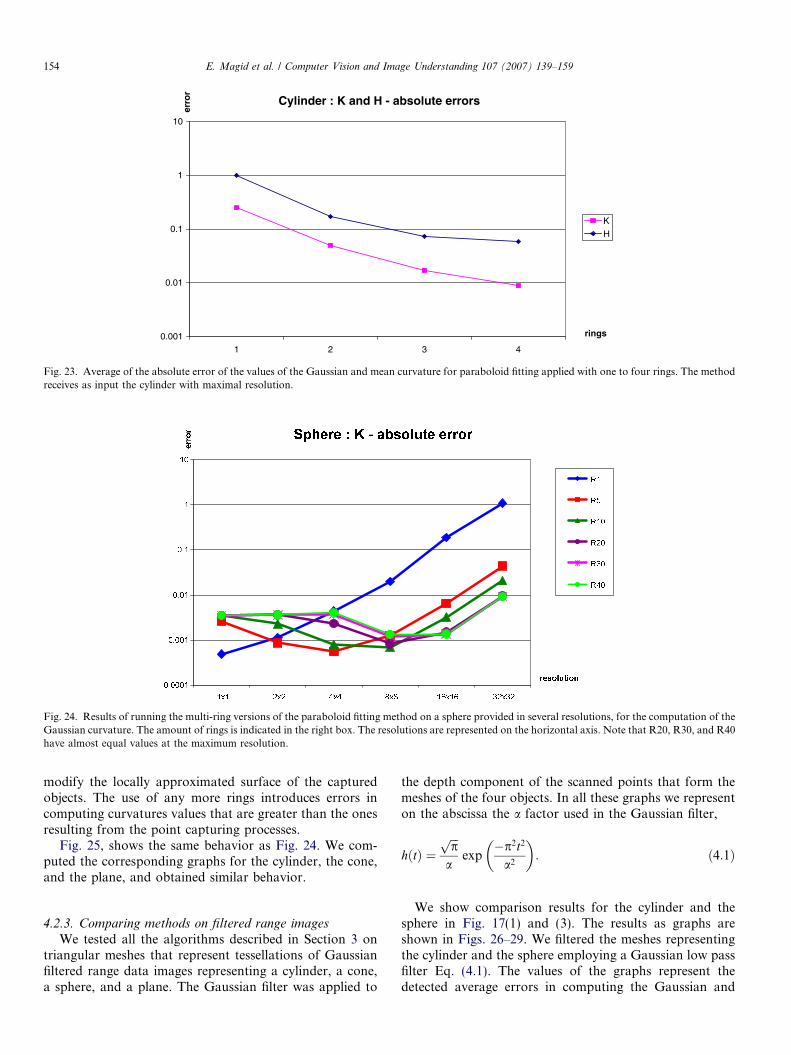
Fig. 24. Results of running the multi-ring versions of the paraboloid fitting method on a sphere provided in several resolutions, for the computation of theGaussian curvature. The amount of rings is indicated in the right box. The resolutions are represented on the horizontal axis. Note that R20, R30, and R40have almost equal values at the maximum resolution.

Cylinder : K and H - absolute errors

0.001

0.01

0.1

1

10

1 2 3 4

rings

erro

r

K

H

Fig. 23. Average of the absolute error of the values of the Gaussian and mean curvature for paraboloid fitting applied with one to four rings. The methodreceives as input the cylinder with maximal resolution.


modify the locally approximated surface of the capturedobjects. The use of any more rings introduces errors incomputing curvatures values that are greater than the onesresulting from the point capturing processes.

Fig. 25, shows the same behavior as Fig. 24. We com-puted the corresponding graphs for the cylinder, the cone,and the plane, and obtained similar behavior.

4.2.3. Comparing methods on filtered range images

We tested all the algorithms described in Section 3 ontriangular meshes that represent tessellations of Gaussianfiltered range data images representing a cylinder, a cone,a sphere, and a plane. The Gaussian filter was applied to

the depth component of the scanned points that form themeshes of the four objects. In all these graphs we representon the abscissa the a factor used in the Gaussian filter,

hðtÞ ¼ffiffiffipp

aexp

�p2t2

a2

� �: ð4:1Þ

We show comparison results for the cylinder and thesphere in Fig. 17(1) and (3). The results as graphs areshown in Figs. 26–29. We filtered the meshes representingthe cylinder and the sphere employing a Gaussian low passfilter Eq. (4.1). The values of the graphs represent thedetected average errors in computing the Gaussian and

Fig. 26. Results of running all the methods on the cylinder, for the computation of the Gaussian curvature. The cylinder model was filtered with aGaussian filter. The horizontal axis represents the radius of the filter whereas the vertical one represents the error. Note that the Gauss–Bonnet and theparaboloid fitting methods have very close values.

Fig. 25. Results of running the multi-ring versions of the paraboloid fitting method on a sphere provided in several resolutions, for the computation of themean curvature. The amount of rings is indicated in the right box. The resolutions are represented on the horizontal axis. Note that R20, R30, and R40have almost equal values at the maximum resolution.


the mean curvatures. Similar graphs were obtained for thecone and the plane.

Figs. 26 and 27 show that all the graphs are monotoni-cally decreasing for a 2 [0..4]. For values of a P 4 thegraphs are non-monotonically decreasing. Moreover, theyare even increasing due to the fact that the Gaussian filtermodifies the objects and thus the values of the Gaussianand the mean curvatures at any point on the meshes. Sim-ilar behavior can be seen in all the graphs; see the addition-al examples in Figs. 28 and 29.

The best method for computing the Gaussian curva-ture when Gaussian filtering is used is Watanabe B.For the mean curvature the best method is WatanabeA. In this context, we mention that the paraboloid fitting

method is one of the best methods for mean curvatureestimation. The four objects analyzed in this sectionare particular geometric objects and the authors feel thatthe paraboloid fitting method is very appropriate, espe-cially on free-form surfaces such as the surface of revo-lution (see Fig. 7(1)) and the spout of the Utah teapot(see Figs. 7(3) and 8). A study on such surfaces requiressolving registration problems and is not in the scope ofthe current work.

Note that in the way in which we applied the Gaussianlow pass filter, the graphs showed convergence of themethods up to point (a � 4), where the surfaces beginto change. Taking into account that Figs. 26 and 27 havelogarithmic scale representations, we conclude that all the

Fig. 28. Results of running all the methods on the sphere, for the computation of the Gaussian curvature. The sphere model was filtered with a Gaussianfilter. The horizontal axis represents the radius of the filter whereas the vertical one represents the error. Note that the Gauss–Bonnet, the paraboloidfitting, the Taubin, and the Taubin B methods have very close values.

Fig. 27. Results of running all the methods on the cylinder, for the computation of the mean curvature. The cylinder model was filtered with a Gaussianfilter. The horizontal axis represents the radius of the filter whereas the vertical one represents the error.


methods received improved input by filtering up to(a � 4). By applying more specialized filters, one canrecover the geometry of scanned objects better. In thiscase, the Gauss–Bonnet scheme remains the best choicefor the Gaussian curvature computation and the parabo-loid fitting method is the best for the mean curvaturecomputation.

Note that especially for the case of the Gaussian curva-ture, the comparison between error results is difficult andperhaps irrelevant when all the methods report very lowvalues. This fact is dictated by numerical reasons such asthe condition numbers of the implied formulas.

4.3. Computation time requirements

We compared the running times of all the algorithmsdescribed in Section 3. Table 2 represents a comparison

of times required for computing the curvatures on the high-est resolution available tessellations for a cylinder, a conus,a sphere, and a plane. The most interesting result relates tothe paraboloid fitting 2 and 3 methods. We measured com-putation times on a personal computer equipped with twoPentium IV hyper-threading 2.4 GHz processors and 1 Gbof memory.

5. Conclusions and future work

In this work, we provided a comparison of four differentapproaches for curvature estimation of triangular meshes.For each approach, we selected a representative algorithm.The input data comprised synthetic geometric objects aswell as range data obtained from scanning real 3D objects.

In the case of synthetic models, the Gauss–Bonnetscheme excels when K is computed and the parabolic fitting

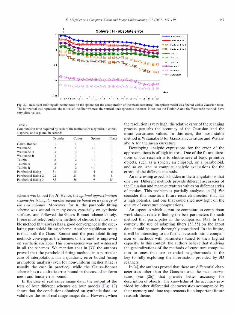
Fig. 29. Results of running all the methods on the sphere, for the computation of the mean curvature. The sphere model was filtered with a Gaussian filter.The horizontal axis represents the radius of the filter whereas the vertical one represents the error. Note that the Taubin A and the Watanabe methods havevery close values.

Table 2Computation time required by each of the methods for a cylinder, a conus,a sphere, and a plane, in seconds

Cylinder Conus Sphere Plane

Gauss–Bonnet 1 1 1 1Watanabe 2 1 <1 1Watanabe A 3 3 1 1Watanabe B 3 3 1 1Taubin 2 2 <1 1Taubin A 2 2 1 1Taubin B 2 2 <1 1Paraboloid fitting 51 15 4 6Paraboloid fitting 2 72 21 6 8Paraboloid fitting 3 85 36 9 15


scheme works best for H. Hence, the optimal approximation

scheme for triangular meshes should be based on a synergy of

the two schemes. Moreover, for K, the parabolic fittingscheme was second in many cases, especially on syntheticsurfaces, and followed the Gauss–Bonnet scheme closely.If one must select only one method of choice, the most sta-ble method that always has a good convergence is the oscu-lating paraboloid fitting scheme. Another significant resultis that both the Gauss–Bonnet and the paraboloid fittingmethods converge as the fineness of the mesh is improvedon synthetic surfaces. This convergence was not witnessedin all the schemes. We mention that in [33] the authorsproved that the paraboloid fitting method, in a particularcase of interpolation, has a quadratic error bound (usingasymptotic analysis) even for non-uniform meshes (that isusually the case in practice), while the Gauss–Bonnetscheme has a quadratic error bound in the case of uniformmesh and linear error bound.

In the case of real range image data, the output of thetests of four different schemes on four models (Fig. 17)shows that the conclusions obtained on synthetic data arevalid over the set of real range images data. However, when

the resolution is very high, the relative error of the scanningprocess perturbs the accuracy of the Gaussian and themean curvatures values. In this case, the most stablemethod is Watanabe B for Gaussian curvature and Watan-abe A for the mean curvature.

Developing analytic expressions for the error of theapproximations is of high interest. One of the future direc-tions of our research is to choose several basic primitiveobjects, such as a sphere, an ellipsoid, or a paraboloid,and so on, and to compute analytic evaluations for theerrors of the different methods.

An interesting aspect is hidden in the triangulations thatone uses. Different methods provide different accuracies ofthe Gaussian and mean curvatures values on different stylesof meshes. This problem is partially analyzed in [6]. Weconsider this issue as a future research direction that hasa high potential and one that could shed new light on thequality of curvature computations.

An aspect to which curvature computation comparisonwork should relate is finding the best parameters for eachmethod that participates in the comparison [43]. In thiscontext, the use of adapting filters [53,55] on the inputdata should be more thoroughly considered. In the future,it will be interesting to do further research into a compar-ison of methods with parameters tuned to their highestcapacity. In this context, the authors believe that studyingthe generalizations of the methods of curvature computa-tion to ones that use extended neighborhoods is thekey to fully exploiting the information provided by 3Dscanners.

In [4], the authors proved that there are differential char-acteristics other than the Gaussian and the mean curva-tures (see [26]) that provide better accuracy fordescription of objects. The knowledge of the accuracy pro-vided by other differential characteristics accompanied bytheir memory and time requirements is an important futureresearch theme.


Acknowledgments

The authors thank Dr. Tatiana Surazhsky and Prof.Gershon Elber for their advice during this research.

References

[1] L. Alboul, R. van Damme, Polyhedral metrics in surface reconstruc-tion: Tight triangulations, in: University of Twente, Department ofApplied Mathematics, Technical Report, Memorandum No. 1275(1995) pp. 309–336.

[2] R. Bergevin, A. Bubel, Detection and characterization of junctions ina 2d image, Computer Vision and Image Understanding 93 (2004)288–309.

[3] P.J. Besl, R.C. Jain, Invariant surface characteristics for 3d objectrecognition in range images, Computer Vision Graphics and ImageProcessing 33 (1986) 33–80.

[4] H. Cantzler, R.B. Fisher, Surface shape and curvature scales, in: TheThird International Conference on 3-D Digital Imaging and Mod-eling, 2001, pp. 285–291.

[5] X. Chen, F. Schmitt, Intrinsic surface properties from surfacetriangulation, in: The Second European Conference on ComputerVision, May 1992, pp. 739–743.

[6] D. Cohen-Steiner, J.-M. Morvan, Restricted delaunay triangulationsand normal cycle, in: Proceedings of the Nineteenth Annual Sympo-sium on Computational Geometry, 2003, pp. 237–246.

[7] G. Dahlquist, A. Bjorck, Numerical methods, Prentice-Hall, Engle-wood Cliffs, New Jersey, 1974.

[8] H. Delingette, General object reconstruction based on simplexmeshes, International Journal of Computer Vision 32 (2) (1999)111–146.

[9] M. DoCarmo, Differential Geometry of Curves and Surfaces,Prentice-Hall, NJ, 1976.

[10] G. Dudek, J.K. Tsotsos, Shape representation and recognition frommultiscale curvature, Computer Vision and Image Understanding 68(2) (1997) 170–189.

[11] N. Dyn, K. Hormann, S. Kim, D. Levin, Optimizing 3d triangula-tions using discrete curvature analysis, in: T. Lyche, L.L. Schumaker(Eds.), Mathematical Methods in CAGD: Oslo 2000, VanderbiltUniversity Press, Nashville, TN, 2001, pp. 135–146.

[12] G. Elber. www.cs.technion.ac.il/~irit/.[13] T.L. Faber, E.M. Stokely, Orientation of 3d structures in medical

images, IEEE Transactions on Pattern Analysis and MachineIntelligence 10 (1988) 626–633.

[14] F.P. Ferrie, M.D. Levine, Deriving coarse 3d models of objects, in:Conference on Computer Vision and Pattern Recognition, June 1988,pp. 345–353.

[15] P.J. Flynn, A.K. Jain, On reliable curvature estimation, in: Confer-ence on Computing Vision and Pattern Recognition, June 1989, pp.110–116.

[16] J.D. Foley, A. van Dam, S.K. Feiner, J.F. Hughes, in: Computergraphics, principles and practice in C, second ed., Addison-WesleyPublishing Company, MA, 1996.

[17] D.B. Goldgof, T.S. Huang, H. Lee, A curvature-based approach toterrain recognition, IEEE Transactions on Pattern Analysis andMachine Intelligence 11 (11) (1989) 1213–1217.

[18] G.H. Golub, C.F.V. Loan, in: Matrix computations, third ed., TheJohns Hopkins University Press, 1996.

[19] M. Gopi, S. Krishnan, C.T. Silva, Surface reconstruction based onlower dimensional localized delaunay triangulation. in: M. Gross,F.R.A. Hopgood (Eds.) Computer Graphics Forum, Eurographics,vol. 19, 3, 2000.

[20] B. Hamann, Curvature approximation for triangulated surfaces,Computing Supplements 8 (1993) 139–153.

[21] E. Hameiri, I. Shimshoni, Estimating the principal curvatures and thedarboux frame from real 3-d range data, IEEE Transactions onSystems, Man and Cybernetics, Part B, Issue 4 33 (2003) 626–637.

[22] A. Hilton, J. Illigworth, T. Windeatt, Statistics of surface curvatureestimates, Pattern Recognition Letters 28 (8) (1995).

[23] http://www.cyberware.com.[24] S.J. Kim, C.-H. Kim, D. Levin, Surface simplification using discrete

curvature norm, in: The Third Israel-Korea Binational Conference onGeometric Modeling and Computer Graphics, Seoul, Korea, October2001.

[25] Y. Kim, R.C. Luo, Validation of 3d curved objects: cad model andfabricated workpiece, IEEE Transactions on Industrial Electronics 41(1) (1994) 125–131.

[26] J. Koenderink, A. van Doorn, Surface shape and curvature scales,Image and Vision Computing 10 (8) (1992) 557–565.

[27] P. Krsek, C. Lukacs, R.R. Martin, Algorithms for computingcurvatures from range data, in: The Mathematics of Surfaces VIII,Information Geometers, in: A. Ball et al. (Eds.), 1998, pp. 1–16.

[28] P. Krsek, T. Pajdla, V. Hlavac, Estimation of differential parameterson triangulated surface, in: The 21st Workshop of the AustrianAssociation for Pattern Recognition, May 1997.

[29] C.-K. Lee, R.M. Haralick, K. Deguchi, Estimation of curvature fromsampled noisy data, in: Conference on Computer Vision and PatternRecognition, 1993, pp. 536–541.

[30] C. Lin, M.J. Perry, Shape description using surface triangulation, in:Proceedings of the IEEE Workshop on Computer Vision: Represen-tation and Control, 1982, pp. 38–43.

[31] R.R. Martin, Estimation of principal curvatures from range data,International Journal of Shape Modeling 4 (1998) 99–111.

[32] A.M. McIvor, J. Valkenburg, A comparison of local surface geometryestimation methods, Machine Vision and Applications 10 (1997) 17–26.

[33] D.S. Meek, D.J. Walton, On surface normal and gaussian curvatureapproximations given data sampled from a smooth surface, Com-puter Aided Geometric Design 17 (6) (2000) 521–543.

[34] F. Mokhtarian, N. Khalili, P. Yuen, Estimation of error in curvaturecomputation on multi-scale free-form surfaces, IEEE Journal ofComputer Vision 48 (2) (2002) 131–149.

[35] O. Monga, S. Benayoun, Using partial derivates of 3d images toextract typical surface features, Computer Vision and Image Under-standing 61 (2) (1995) 171–189.

[36] S.M. Naik, R.C. Jain, Spline-based surface fitting on range images forcad applications, in: Conference on Computer Vision and PatternRecognition, June 1988, pp. 249–253.

[37] D.L. Page, Y. Sun, J. Paik, M.A. Abidi, Normal vector voting: Creasedetection and curvature estimation on large, noisy meshes, GraphicalModels 64 (2002) 199–229.

[38] U. Pinkall, K. Polthier, Computing discrete minimal surfaces andtheir conjugates, Experimental Mathematics 2 (1) (1993) 15–36.

[39] K. Polthier, M. Schmies, Straightest geodesics on polyhedral surfaces,in: K. Polthier, H.C. Hege (Eds.), Mathematical Visualization,Springer-Verlag, Berlin/New York, 1998, pp. 391–409.

[40] F.K.H. Quek, R.W.I. Yarger, C. Kirbas, Surface parametrization involumetric images for curvature-based feature classification, IEEETransactions on Systems, Man, and Cybernetics 33 (5) (2003) 758–765.

[41] C. Rosl, L. Kobbelt, H. Seidel, Extraction of feature lines ontriangulated surfaces using morphological operators, in: SmartGraphics, AAAI Symposium, 2000, pp. 71–75.

[42] P.T. Sanders, S.W. Zucker, Inferring surface trace and differentialstructure from 3d images, IEEE Transactions on Pattern Analysis andMachine Intelligence 12 (9) (1990) 833–854.

[43] A.J. Stoddart, J. Illingworth, T. Windeatt, Optimal parameterselection for derivative estimation from range images, Image andVision computing 13 (8) (1995) 629–635.

[44] E.M. Stokely, S.Y. Wu, Surface parameterization and curvaturemeasurement of arbitrary 3d-objects: five practical methods, IEEETransactions on Pattern Analysis and Machine Intelligence 14 (8)(1992) 833–840.

[45] D. Struik, Lectures on Classical Differentional Geometry, Addison-Wesley Series in Mathematics (1961).

[46] T. Surazhsky, E. Magid, O. Soldea, G. Elber, E. Rivlin. A comparisonof gaussian and mean curvatures estimation methods on triangular

http://www.cs.technion.ac.il/~irit/

http://www.cyberware.com


meshes, in: International Conference on Robotics and Automation(ICRA2003), Taipei, Taiwan, 14–19 September 2003, pp. 1021–1026.

[47] C.-K. Tang, G. Medioni, Curvature-augmented tensor voting forshape inference from noisy 3d data, IEEE Transactions on PatternAnalysis and Machine Intelligence 24 (6) (2002) 858–864.

[48] C.-K. Tang, G. Medioni, M.-S. Lee, N-dimensional tensor voting andapplication to epipolar geometry estimation, IEEE Transactions onPattern Analysis and Machine Intelligence 23 (8) (2001) 829–844.

[49] G. Taubin, Estimating the tensor of curvature of a surface from apolyhedral approximation, in: The Fifth International Conference onComputer Vision, 1995, pp. 902–907.

[50] J.P. Thirion, A. Gourdon, Computing the differential characteristicsof isointensity surfaces, Computer Vision and Image Understanding61 (2) (1995) 190–202.

[51] W.S. Tong, C.-K. Tang, Robust estimation of adaptive tensors ofcurvature by tensor voting, IEEE Transactions on Pattern Analysisand Machine Intelligence 27 (3) (2005) 434–449.

[52] E. Trucco, R.B. Fisher, Experiments in curvature-based segmentationof range data, IEEE Transactions on Pattern Analysis and MachineIntelligence 17 (2) (1995) 177–182.

[53] L.J. van Vliet, I.T. Young, P.W. Verbeek, Recursive gaussianderivative filters. in: Proceedings of the 14th International Conferenceon Pattern Recognition, vol. 1, August 1998, pp. 509–514.

[54] K. Watanabe, A.G. Belyaev, Detection of salient curvature featureson polygonal surfaces, in: Eurographics 2001, vol. 20, No. 3, 2001.

[55] I.Weiss,High-orderdifferentiation filters thatwork, IEEETransactionson Pattern Analysis and Machine Intelligence 16 (7) (1994) 734–739.

[56] K. Wu, M.D. Levine, 3d part segmentation using simulated electricalcharge distributions, IEEE Transactions on Pattern Analysis andMachine Intelligence 19 (11) (1997) 1223–1235.

[57] S.M. Yamany, A.A. Farag, Surface signatures: an orientationindependent free-form surface representation scheme for the purposeof objects registration and matching, IEEE Transactions on PatternAnalysis and Machine Intelligence 24 (8) (2002).

a comparison of gaussian and mean curvature estimation ...ehudr/publications/pdf/magidsr07a.pdf ·...

Documents